Article

Opportunity-Maintenance-Based Scheduling Optimization for Ship-Loading Operation Systems in Coal Export Terminals

State Key Laboratory of Coastal and Offshore Engineering, Dalian University of Technology, Dalian 116024, China
*
Author to whom correspondence should be addressed.
J. Mar. Sci. Eng. 2024, 12(8), 1377; https://doi.org/10.3390/jmse12081377
Submission received: 22 July 2024 / Revised: 7 August 2024 / Accepted: 10 August 2024 / Published: 12 August 2024

Abstract

:
As important nodes of the global coal supply chain, coal export terminals bear the tasks of coal storage, processing, and handling, whose efficiency and stability are of great importance with the growing coal shipping market in recent years. However, poor working conditions of the handling equipment in the coal export terminal, together with its relatively fixed layout and poor flexibility, allow frequent equipment failures to seriously affect the ship-loading operations. To solve the problem, this paper constructs a scheduling optimization model for ship-loading operation systems considering equipment maintenance and proposes an opportunity-maintenance-based two-layer algorithm to solve the model. The upper layer aims to optimize the scheduling scheme of the ship-loading operation system under a certain maintenance plan. The lower layer of the algorithm, an opportunity-maintenance-based “equipment-level–flow-level” maintenance optimization method, determines the best equipment maintenance plan. A coal export terminal in China is employed as the case study to verify the effectiveness of the proposed method. The results show that the proposed method can reduce the average dwell time of ships at the terminal by 15.8% and save total scheduling and maintenance costs by 10.3%. This paper shows how to make full use of equipment failure historical data and integrate equipment maintenance schemes into the scheduling problem of the ship-loading operation system, which can effectively reduce the impact of equipment failures on ship-loading operations and provide decision support for coal export terminal management.

1. Introduction

With the continuous increase in demand for coal and iron ore, the global dry bulk shipping market is developing strongly. According to the market research forecast, the global dry bulk shipping market will grow at a compound annual rate of 4% from 2022 to 2030, which will reach 547.971 billion U.S. dollars by 2030. As an important energy and strategic material, coal is mostly transported by sea. Coal ports, which are an important node of the coal supply chain, bear the important tasks of coal storage, processing, and handling. Therefore, ensuring the handling efficiency of coal ports is crucial to the stability of the coal supply chain.
At present, the working conditions of coal terminals are relatively poor, and the handling equipment often runs continuously under high load and high power, leading to frequent failures. According to statistics, at China’s main coal export port Huanghua Port, equipment downtime due to equipment failures and other reasons accounts for 20.5% of the total handling operations duration. Meanwhile, compared with other types of terminals (e.g., container terminals and general cargo terminals), horizontal transportation of coal terminals is completed by belt conveyors and other continuous operating equipment, whose layout is relatively fixed, with a strong correlation between handling equipment and poor flexibility. The failure of the handling equipment will lead to the stagnation of the terminal’s entire handling operation.
Furthermore, compared with the coal import terminals, the upstream industry of coal export terminals is usually more concentrated, and the goods are often loaded at several specific terminals and then transported to the destination port by water. As a result, the coal export terminals have a higher degree of specialization and larger transportation volume, lending the handling stagnation a greater impact on the entire coal supply chain. Therefore, putting forward a reasonable maintenance method of handling equipment to reduce the ship waiting time caused by the maintenance of handling equipment is of great significance to improve the handling efficiency of coal export terminals and the stability of the coal supply chain.
This paper aims to solve the scheduling optimization problem of ship-loading operation systems in coal terminals considering handling equipment maintenance, and a two-layer solution algorithm is proposed to support managers in making reasonable scheduling and maintenance decisions. The main contributions are as follows:
First of all, to the best of our knowledge, this is the first work to consider the impact of equipment failure and maintenance when addressing coal terminal handling operations. The interaction between scheduling and maintenance of handling equipment is further elucidated by considering the constraints of complex decision-making caused by equipment maintenance.
Secondly, an opportunity maintenance (OM)-based algorithm is developed to optimize the ship operation sequence, handling operation sequence, and equipment maintenance plan at the same time. Specifically, the lower layer of the algorithm makes full use of equipment failure historical data and introduces opportunity maintenance to obtain an equipment-level and flow-level optimal maintenance plan step by step, considering the series-parallel relationship between equipment. The upper layer optimizes the scheduling scheme of the ship-loading operation system under a certain maintenance plan obtained from the lower layer.
Finally, the validity and practicability of the proposed method are verified by taking the ship-loading operation system in a coal terminal in north China as an example.
The remainder of this paper is organized as follows. Section 2 reviews the related studies. Section 3 describes the studied system and problem, builds the mathematical model, and describes the solution algorithm. Section 4 conducts numerical experiments, followed by Section 5 which summarizes the whole paper and puts forward the future research direction.

2. Literature Review

The existing studies related to this paper can be divided into three parts: dry bulk terminal operating system scheduling, port infrastructure operation and maintenance, and opportunity maintenance.

2.1. Dry Bulk Terminal Operating System Scheduling

At present, the research of operating system scheduling in dry bulk cargo terminals can be divided into three parts: yard scheduling, berth allocation, and multi-system joint scheduling.
In the study of storage yard scheduling, some scholars devote themselves to the development of storage plans. Ouhaman et al. studied a real-world storage space allocation problem at an export bulk terminal [1]. Xin et al. proposed a modeling and control methodology for allocating materials in a dry bulk terminal [2]. Savelsbergh and Smith proposed a tree search algorithm for managing the stockyard at a coal export terminal considering coal assembly planning [3]. Burdett et al. proposed a new method to characterize the stockpiles in dry bulk terminals called bench block models [4]. Angelelli et al. and Kalinowski et al. provided constant-factor approximation algorithms and exact branch-and-bound algorithms to solve the scheduling problem of reclaimers in the stockyard of a coal export terminal [5,6]. Belassiria et al. developed a branch-and-bound method to solve the stacker and reclaimer scheduling problem in the coal storage area [7]. van Vianen et al. proposed a simulation-based method to schedule the stacker–reclaimer operation in a dry bulk yard [8]. Hu et al. proposed a genetic algorithm for stacker–reclaimer scheduling in an iron ore terminal [9]. Unsal et al. studied a complex parallel scheduling problem with non-crossing constraints, sequence-dependent setup times, and eligibility restrictions [10].
In the study of berth allocation, Ernst et al. proposed a two-phase method for solving the berth allocation problem in dry bulk terminals [11]. Cheimanoff et al. proposed a reduced VNS-based approach to solving the dynamic continuous berth allocation problem in bulk terminals considering tidal constraints [12]. de Leon et al. developed a machine-learning-based system for berth scheduling at bulk terminals [13]. Hu et al. established the mathematical model of berth allocation strategies considering the quayside’s limitation and the loading capacity of ships [14]. Guo et al. developed an integrated scheduling model managing the scheduling process of vessel traffic and deballasting operations [15].
Some researchers also study the integrated scheduling problem of the yard operating system and dock operating system. Burdett et al. presented an improved scheduling approach for optimizing the activities of a coal export terminal (CET) [16]. Belov et al. developed a metaheuristic logistics planning system integrating train scheduling, stockpile management, and vessel scheduling [17]. Burdett et al. modeled CET as a flexible job shop with operators and used an advanced meta-heuristic algorithm to solve the model [18]. de Andrade et al. proposed a mixed-integer linear programming formulation to deal with the integration problem in dry bulk export port terminals [19]. Unsal and Oguz proposed a logic-based Benders decomposition algorithm to solve the problem consisting of berth allocation, reclaimer scheduling, and stockyard allocation [20]. Menezes et al. presented a hierarchical approach to solve the production planning and scheduling problem in bulk cargo terminals [21]. Jiang et al. studied an optimization problem of integrated scheduling of restricted channels, berths, and yards in bulk cargo ports considering carbon emissions [22].
The mathematical model and solution algorithms proposed in these studies are important references for this study. However, these studies did not consider the impact of handling equipment failures on schedule, making them unsuitable to be used in this study.

2.2. Port Infrastructure Operation and Maintenance

In terms of port infrastructure operation and maintenance, some scholars studied the impact of infrastructure disruption caused by extreme weather (hurricanes, etc.) on ports [23], while few studies have studied the impact of equipment failure on port operation. Lewandowski and Scholz-Reiter proposed a framework for the systematic design and operation of condition-based maintenance systems [24]. Widarto and Handani developed the maintenance scheduling for the diesel generator support system of the container crane [25]. Mhalla et al. proposed a selective maintenance scheme combining failure rate and age for container port handling equipment [26]. Szpytko and Duarte developed a conceptual model of maintenance decisions for container terminal cranes based on digital twins [27]. Lin et al. built an age-reduction maintenance model to describe the deterioration situation of the port facility [28]. Tchotang et al. combined the Pareto method and trend test to analyze the reliability of a reach stacker [29]. Zheng et al. studied an integrated berth allocation, quay crane assignment, and specific quay crane assignment problem where quay crane maintenance is involved [30]. Krimi et al. proposed a mixed-integer programming model and investigated a set of heuristics algorithms based on general variable neighborhood search [31]. Sepehri et al. analyzed historical automatic identification system data to identify the interaction between maintenance dredging and seagoing vessels and quantify the hindrance periods for the case study in the Port of Rotterdam [32].
It can be seen that most of these studies focus on handling equipment in container ports, such as quay cranes, stackers, etc. However, since the handling operation conditions of coal terminals are different from those of container terminals, these studies cannot be used in this study.

2.3. Opportunity Maintenance

Opportunity maintenance (also called opportunistic maintenance), which reduces maintenance costs or time by combining the maintenance of multiple components, has been widely used in complex systems (e.g., wind turbines, PV power generation systems, CNC gear grinding machines) and has been attracting wide attention from researchers in recent years [33]. Huang et al. proposed a condition-based opportunistic maintenance policy for series systems with dependent competing failure processes [34]. Li et al. developed a maintenance optimization model designed for a system comprising two distinct components that are arranged in series and susceptible to common-cause failure [35]. Su et al. presented a condition-based opportunistic maintenance strategy for multi-component wind turbines by using stochastic differential equations [36]. To solve the problem of the high maintenance cost of PV power generation systems due to unreasonable opportunity maintenance grouping, Chen et al. proposed an opportunity maintenance strategy for PV power generation systems considering the structural relevance [37]. Wang et al. presented a novel optimal opportunistic maintenance strategy for wind turbines considering wind speed as a stochastic process [38]. Chen et al. studied an opportunistic maintenance optimization problem of continuous process manufacturing systems considering imperfect maintenance with epistemic uncertainty [39]. Dinh et al. developed an opportunistic predictive maintenance framework for a system comprising one continuous-operation component and an intermittent-operation component [40]. Dinh et al. discussed how disassembly actions can affect the system reliability and opportunistic maintenance optimization of disassembled components in a multicomponent system subjected to structural dependence [41]. Li et al. studied an opportunistic maintenance strategy optimization problem for a CNC gear grinding machine considering imperfect maintenance under a hybrid unit-level maintenance strategy [42]. Wei et al. proposed an optimal opportunistic maintenance planning for the critical structure of circulating pumps integrating discrete- and continuous-state information [43]. Chen et al. developed an opportunistic maintenance strategy for PV power generation systems under the action of random shocks [44]. Li et al. studied the influence mechanism of the interaction between operation and maintenance activities within the whole life cycle of electric multiple-unit components on the maintenance strategy, based on the concept of lean maintenance [45]. Yuan et al. presented an opportunistic maintenance model of multi-component complex systems based on a time threshold, with the consideration of the disassembly sequence and hybrid evolution factors influencing maintenance and learning–forgetting effects [46].
Most of the studies above focus on series systems instead of series-parallel systems, and few of them consider the interaction between maintenance and scheduling of the system, making them unsuitable to be used to solve the maintenance-based scheduling optimization problem for a ship-loading operation system, which is a series-parallel system.

3. Research Methods

In this section, the problem discussed in this paper is first presented in Section 3.1. The method of building the optimization model is then expressed in Section 3.2, followed by the proposed OM-based two-layer algorithm in Section 3.3.

3.1. Problem Description

This paper attempts to solve the scheduling optimization problem of the ship-loading operation system, considering equipment maintenance; the complexity of the problem is detailed in the following subsection.

3.1.1. Scheduling of Ship-Loading Operation System

As shown in Figure 1, after a ship arrives at the berth, the corresponding reclaimers (R) are invoked to unload the coal at the storage yard according to the operation plan. Then, the coal is transported to the front of the terminal via a series of belt conveyors including BQ, BC, and BM. Finally, the corresponding ship loader (SL) is called to complete the dry bulk cargo loading operation.
The complexity of shipping operation system scheduling is mainly reflected in the following aspects: (1) a ship with multiple tasks; (2) mixing operation of reclaimers; (3) combined operation of ship-loaders; and (4) uniqueness and accessibility constraints.

3.1.2. Maintenance of Equipment in the Ship-Loading Operation System

The handling equipment in the ship-loading operation system, including reclaimers, belt conveyors, and ship-loaders, may be in a series or parallel relationship (see the red dashed line in Figure 1). In this study, based on the characteristics of scheduling and maintenance of handling equipment in coal export terminals, its maintenance is treated as follows.
(1)
Repairable equipment. When the handling equipment encounters failure, it is repaired rather than replaced.
(2)
Predictive maintenance of handling equipment. After the handling equipment of the ship-loading operation system is put into use for some time, its failure rate will increase. In this case, predictive maintenance (PdM, i.e., maintenance according to the status of the handling equipment) should be carried out to restore the failure rate of the handling equipment to a lower layer. The normal working duration between two PdMs is called the predictive maintenance interval (PdMI), and the time of each PdMI is recalculated from 0 and denoted as (0, Tij), where j is the number of PdMs. Tij is denoted as the predictive maintenance interval length (PdMIL).
(3)
Minimal repair of handling equipment. For the handling equipment faults occurring between two PdMs, the concept of minimal repair is introduced. The duration of minimal repair is shorter than that of PdM, and will not change the failure rate of the handling equipment, but only restore the handling equipment to the state before its failure.

3.2. Model Establishment

The basic assumptions, notations, objective function, and constraints of the optimization model are introduced as follows.

3.2.1. Basic Assumptions and Notations

The basic assumptions of the optimization model are shown as follows:
(1)
The time of the ship arriving at the terminal and the arranged berth are known.
(2)
The ship’s time at the terminal counts from the ship arriving at the berth to the ship leaving the berth.
(3)
The pile to reclaim, amount of reclaiming, and operation duration of ship-loading task are known.
(4)
Before a ship-loading task is finished, the operation line occupied cannot be used for other tasks.
(5)
The parameters in the failure rate evolution function have been obtained by fitting historical data. The age and status of the handling operation equipment are known as well. The notations used in the model are shown in Table 1.

3.2.2. Objective Function

M i n   C t o t a l = C t i m e + C e n e r g y + C m a i n t e n a n c e
C t i m e = s S t s d e p t s a r r × E s s h
C e n e r g y = m M [ u U E u b q × y m , u b q + v V E v b c × y m , v b c + w W E w b m × y m , w b m × d m + u U A u b q × a m , u b q × y m , u b q + v V A v b c × a m , v b c × y m , v b c + w W A w b m × a m , w b m × y m , w b m ]
C m a i n t e n a n c e = m M i I m N i m × E i s m + j N i m N i m j × E i m j u m
The objective function is the total cost of maintenance and scheduling for ship-loading operation system C t o t a l , consisting of dwell time cost of ships C t i m e , energy consumption cost of operation lines C e n e r g y , and handling equipment maintenance cost C m a i n t e n a n c e . C t i m e mainly considers the easing cost of ships, which is determined by the well time of ship s at port t s d e p t s a r r , and cost per unit time E s s h . C e n e r g y consists of transportation energy cost and start-up energy cost. Transportation energy cost is calculated by unit cost of reclaiming operation line u U E u b q × y m , u b q , unit cost of horizontal operation v V E v b c × y m , v b c , unit cost of ship-loading operation w W E w b m × y m , w b m , and coal required by ship-loading task m, d m . Start-up energy cost considers cost of idling during the start-up phase of three operating lines u = 1 U A u b q × a m , u b q × y m , u b q , v = 1 V A v b c × a m , v b c × y m , v b c , and w = 1 W A w b m × a m , w b m × y m , w b m . C m a i n t e n a n c e considers PdM cost N i m × E i s m and minimal repair cost j = 1 N i m N i m j × E i m j u m .

3.2.3. Constraints

(1)
Constraints connecting ships mooring and leaving the berths
z s , s s h + z s , s s h = k K β s , k × β s , k , s , s S , s s
t s a r r t s d e p M × 1 z s , s s h , s , s S , s s
t s d e p = m a x m t m s + τ m t a + τ m d o w n × θ s , m + τ s u n , s S
t m s + M × 1 θ s , m t s a r r + τ s a u x , s S , m M
Equation (5) indicates that ships with higher priority occupy the berth preferentially. In the equation, z s , s s h is a 0–1 variable, whose value is 1 if the priority of ship s is higher than that of ship s , 0 otherwise. k is the serial number of berth k = 1 , 2 , , K , while K is the total number of berths in the terminal. β s , k is the 0–1 variable, whose value is 1 if berth k is occupied by ship s, 0 otherwise. Equation (6) indicates that the mooring time of any ship should be later than the departure time of the previous ship at corresponding berth, where M is a sufficiently large positive real number. Equation (7) indicates that the ship can leave the berth after completing all of its ship-loading tasks, where t m s , τ m t a , and τ m d o w n are the start time, operating duration, and maintenance duration of task m, respectively. θ s , m is a 0–1 variable, whose value is 1 if task m belongs to ship s, 0 otherwise. τ s u n is the unmoor duration of ship s. Equation (8) indicates that the ship can only start handling operations after completing auxiliary operations, whose duration is τ s a u x .
(2)
Constraints connecting ship-loading tasks
z m , m t a + z m , m t a = m a x p , u , v , w γ m , p , γ m , p , y m , u b q , y m , u b q , y m , v b c , y m , v b c , y m , w b m , y m , w b m , ε m , m , m , m M , m m
ε m , m = k K δ m , k × δ m , k × w = 2 W 1 y m , w 1 b m × y m , w + 1 b m + y m , w 1 b m × y m , w + 1 b m , m , m M , m m
t m s t m s + τ m t a + τ m d o w n M × 1 z m , m t a + φ m , m , m , m M , m m
φ m , m = w W y m , w b m × y m , w b m × k K k K δ m , k × δ m , k × π k , k + ε m , m × η , m , m M , m m
t + M × 1 x m , t t a t m s , m M , t T
t M × 1 x m , t t a < t m s + τ m t a + τ m d o w n , m M , t T
t T x m , t t a = τ m t a + τ m d o w n , m M
Equation (9) represents the priority that two loading tasks m and m should meet, which occupy the same pile, the operation lines, or two ship-loaders on either side of the same berth, where z m , m t a is a 0–1 variable, whose value is 1 when priority of task m is higher than task m , 0 otherwise. p is the serial number of pile p = 1 , 2 , , P . γ m , p is a 0–1 variable, whose value is 1 if task m unloads coal from pile p, 0 otherwise. ε m , m is a 0–1 variable representing the relationship between two tasks occupying two ship-loaders on either side of the same berth, 1 if tasks m and m meet the condition, 0 otherwise. ε m , m can be calculated by Equation (10), where δ m , k is 0–1, whose value is 1 if task m is finished by the ship mooring at berth k, 0 otherwise. Equation (11) represents the start time constraints of two ship-loading tasks with priority constraint, where φ m , m is the operation time interval between task m and m , considering the possible operating time of the ship-loader shifting, as well as the operating time interval of two tasks occupying two ship-loaders on either side of the same berth (see Equation (12)). π k , k is the duration to move the ship loader from berth k to k , while η means operating time interval. Equations (13)–(15) indicate that the same task cannot be interrupted, except for predictive maintenance and minimal repairs during the operation. Note that the time is discretized in this paper, thus t = 1 , 2 , T , and T is the optimization period length. x m , t t a is a 0–1 variable, whose value is 1 if task m is in progress at time t, 0 otherwise.
(3)
Constraints connecting the handling equipment selection
u U y m , u b q × v V y m , v b c × w W y m , w b m = 1 , m M
y m , u b q p P p = 0 p 1 γ m , p × γ m , p × α p , p , u b q , m M , u U
y m , v b c u U w W y m , u b q × y m , w b m × α u , v , w b c , m M , v V
y m , w b m k K δ m , k × α w , k b m , m M , w W
m M k K x m , t t a × y m , w b m × δ m , k × k m M k K x m , t t a × y m , w b m × δ m , k × k + M × 1 m M x m , t t a × y m , w b m , t T , w , w W , w < w
Equation (16) indicates that a ship-loading task requires only one reclaiming operation line, horizontal operation line, and ship-loading operation line, respectively. Equations (17)–(19) indicate that there are accessibility constraints among the pile, reclaiming operation line, horizontal operation line, ship-loading operation line, and berth occupied by task, where α p , p , u b q is a 0–1 variable, whose value is 1 if reclaiming operation line u can access pile p and p , 0 otherwise. Note that p is the serial number of the pile that is used for mixing operation with pile p. When p = 0 , pile p is used for reclaiming operation only. α u , v , w b c is a 0–1 variable, whose value is 1 if horizontal operation line v can access reclaiming operation line u and ship-loading operation line w, 0 otherwise. Similarly, α w , k b m is a 0–1 variable, whose value is 1 if ship-loading operation line w can access berth k, 0 otherwise. Equation (20) indicates that the ship-loaders cannot cross each other.
(4)
Constraints connecting the PdM and minimal repair
2 × u U a m , u b q × y m , u b q + v V a m , v b c × y m , v b c + 2 × w W a m , w b m × y m , w b m = i I m N i m + j N i m N i m j + 1 , m M
j = 1 N i m 1 T i m j < τ m t a j = 1 N i m T i m j
i I p j N i m T i m j T i P m i n i I p T i m j < τ m t a
τ m t a i I p j N i m T i m j T i P
Equation (21) indicates that start-up times of the occupied operation line m should correspond to the number of PdMs and minimal repairs included in the operation line. Equation (22) indicates the relationship between the number of PdMs of handling equipment i during ship-loading task m (denoted as N i m ) and the PdMIL of equipment i in that period (denoted as T i m j ) when equipment i is not paralleled with other equipment. Similarly, Equations (23) and (24) indicate the relationship between N i m and T i m j when equipment i is paralleled with other equipment, where I p is the set of equipment in the parallel part of equipment i, i I p . T i P is the duration when equipment i and its paralleled equipment work simultaneously.

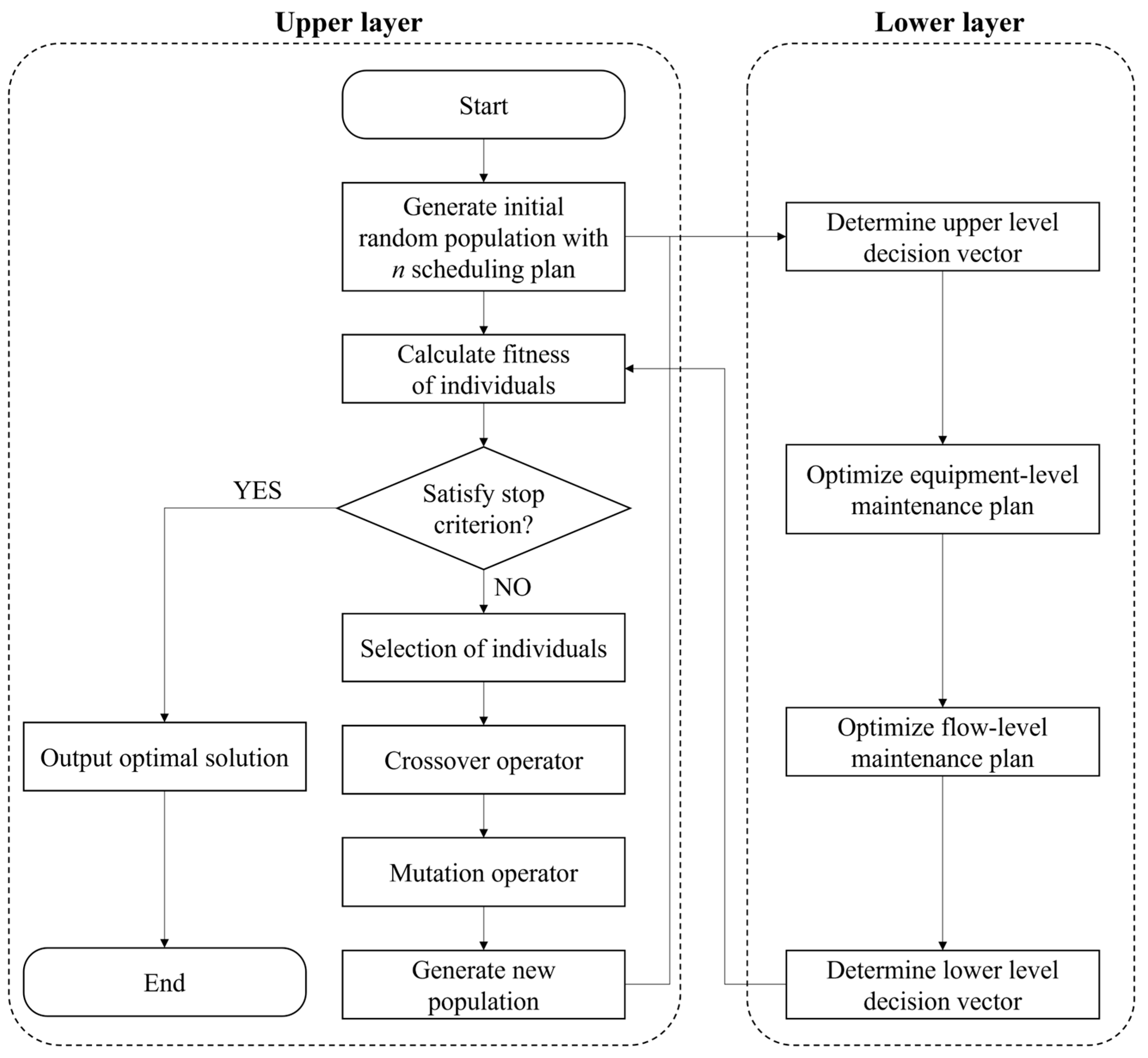
3.3. OM-Based Two-Layer Algorithm

To solve the scheduling optimization model for the ship-loading operation system considering equipment maintenance, this paper proposes an OM-based two-layer algorithm.

3.3.1. Algorithm Framework

As shown in Figure 2, the upper layer of the algorithm is used to determine the optimal scheduling plan of the system, while the lower layer optimizes the maintenance plan and feedback to the upper layer.

3.3.2. Upper Layer

The upper layer is a genetic algorithm (GA), whose objective is to minimize C t o t a l . It is used to determine the scheduling plan of the ship-loading operating system under a specific equipment maintenance plan.
(1)
Chromosome coding
The chromosome coding of GA is shown in Table 2. Where b i is the berthing priority of ship i at the corresponding berth, the smaller the value of b i , the higher the berthing priority. Similarly, c j represents the operation priority of the ship-loading task j. The smaller the value, the higher the operation priority. e j , f j , and g j are the serial numbers of the reclaiming operation line, horizontal operation line, and ship-loading operation line occupied by task j, respectively.
(2)
Population initialization
The rules for generating the initial population are as follows.
(a)
The berthing priority of the ship’s sequence is randomly generated according to the ship’s assigned berth.
(b)
After the priority sequence of the ship-loading task is randomly generated, it is adjusted according to the berthing priority of the ship to which the task belongs. The higher the berthing priority, the higher the priority of the ship-loading task.
(c)
The sequence of reclaiming operation line and ship-loading operation line sequence is randomly selected when the accessibility requirements of berth and stack are met.
(d)
The horizontal operation line sequence is randomly selected to meet the accessibility requirements of the reclaiming operation line and ship-loading operation line.
(3)
Fitness function selection
C t o t a l is selected as the fitness function.
(4)
Genetic operator
(a)
Genetic operator selection: the roulette method is used first to select a certain number of chromosomes from the parents for crossover and mutation operations, to produce offspring individuals. After that, the optimal strategy is adopted to select the fitter individuals in the parents and offspring to carry out the next generation of genetic operation, to retain all the excellent individuals in the evolution process.
(b)
Crossover strategy: The overall single-point crossover is adopted as the crossover strategy, the five sequences are crossed at the same time, and the following three possible new chromosome situations that do not meet the constraint conditions are corrected:
In the berthing priority-of-ships sequence, if the berthing priorities of two ships in the same berth are equal, one of the repeated priorities is randomly selected and replaced with the missing priority in the sequence.
In the priority of ship-loading task sequence, if the priority of two tasks is equal, the amendment principle is the same as ①.
Between the priority of ship-loading task sequence and the berthing priority of ship sequence, if the priority of the task of the ship with low priority is higher than that of the ship with high priority at the same berth, it will be adjusted.
(c)
Mutation strategy: Three mutation strategies are adopted, and the adoption probabilities of the three mutation strategies are 0.4, 0.3, and 0.3, respectively.
The gene locations of two ships berthing at the same berth are randomly selected and their berthing priorities are exchanged. If there is a contradiction between the priority of ship-loading task sequence and berthing priority-of-ship sequence, it will be adjusted according to the berthing priority of the corresponding ship-loading task. The higher the berthing priority, the higher the priority of the ship-loading task.
In the ship-loading task priority sequence, two genes are randomly selected for exchange, whose correction principle is the same as ①.
The gene location of the ship-loading operation line sequence is randomly selected and replaced by another ship-loading operation line occupied by the same task. If the accessibility constraint between the new ship-loading operation line and the original horizontal operation line is not satisfied, a new horizontal operation line is randomly selected to meet the accessibility constraint for correction.
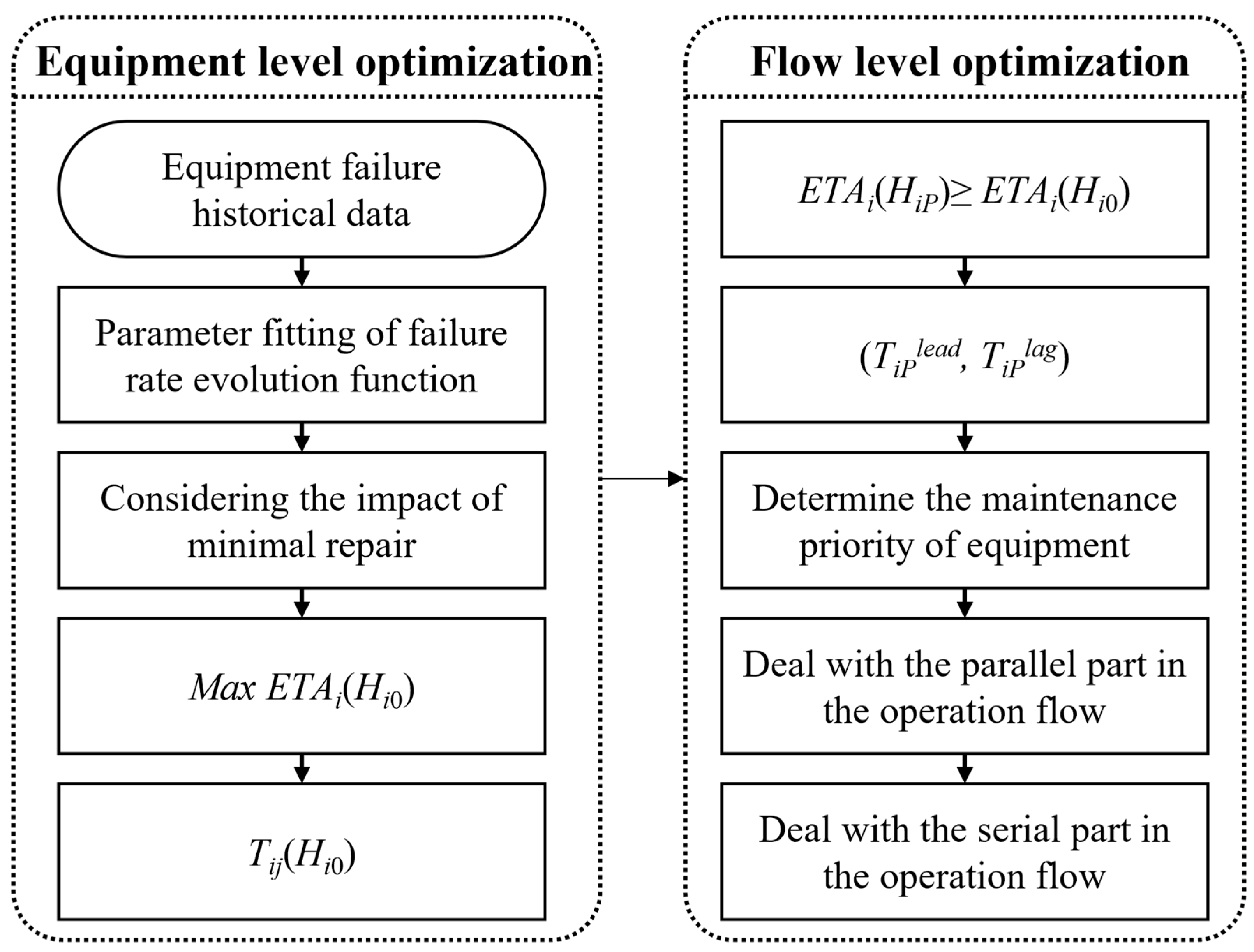
3.3.3. Lower Layer

The lower layer is an OM-based equipment maintenance method, which is used to obtain optimal equipment maintenance plans under a specific scheduling plan. The objective function of the lower layer is to minimize τ m d o w n , which can also be expressed as Equation (25) since τ m t a is fixed.
E T A m = τ m t a τ m t a + τ m d o w n
The proposed OM-based “equipment-level–flow-level” maintenance optimization method is shown in Figure 3.
(1)
Failure rate evolution function modeling
Considering the impact of the increased failure rate caused by the external environment, the increased failure rate caused by wear and tear, and the imperfect maintenance of handling equipment, the failure rate evolution function of equipment i can be modeled by Equation (26).
f i j + 1 t = γ i β i f i j t + a i T i j , t 0 , T i j + 1 , j = 1 , 2 , , N i
where γ i is the environmental factor, β i is the failure rate factor, a i is the recursively decreasing factor, and γ i > 1 , β i > 1 , 0 < a i < 1 . N i is the number of PdMIs for equipment i in its life cycle. In this paper, T i j T i 1 is used as the parameter to judge whether to replace equipment i. When T i j T i 1 C , C ( 0 , 1 ) is satisfied for the first time, equipment i will be replaced and the corresponding j is recorded as N i , and the replacement of equipment i is treated as its N i th PdM. T i j is jth PdMIL of equipment i, T i j = t i j s m s t i j 1 s m e , where t i j s m s is the start time of jth PdM of equipment i, t i j 1 s m e is the end time of the (j − 1)th PdM of equipment i, and t i 0 s m e is the time when equipment i is put to use. Thus, the cumulative failure rate function of equipment i at time t in its jth PdMI, F i j t , can be expressed as follows.
F i j t = 0 t f i j x d x
For repairable equipment i, the concept of failure rate threshold is introduced to ensure its stable working state. The failure rate threshold of equipment i in its jth PdMI, H i 0 , is defined. Once the cumulative failure-rate function of equipment i in its jth PdMI reaches H i 0 , PdM should be performed.
H i 0 = 0 T i j f i j t d t = F i j T i j
(2)
Failure rate evolution function parameter fitting
According to the historical data, the failure rate evolution function of the equipment is fitted to a three-parameter Weber distribution, shown in Equation (29).
λ i j t = η i j θ i j t t i j 0 θ i j η i j 1 , t 0 , T i j , j = 1 , 2 , , N i
Then, Equation (26) can be expressed as follows.
f i j t = η i j θ i j t t i j 0 θ i j η i j 1 , t 0 , T i j , j = 1 γ i β i f i j 1 t + a i T i j 1 , t 0 , T i j , j = 2 , 3 , , N i
When j = 1, f i 1 t is the first term of the recursion formula of f i j t , thus f i 1 t = λ i 1 t . When j > 1 , f i j t meet Equations (26) and (29) at the same time, thus f i j t = γ i β i f i ( j 1 ) t + a i T i ( j 1 ) = λ i j t . Furthermore, let j = 2 and 3, Equations (31) and (32) can be obtained.
γ i β i η i 1 θ i 1 t t i 1 0 + a i T i 1 θ i 1 η i 1 1 = η i 2 θ i 2 t t i 2 0 θ i 2 η i 2 1
γ i β i η i 2 θ i 2 t t i 2 0 + a i T i 2 θ i 2 η i 2 1 = η i 3 θ i 3 t t i 3 0 θ i 3 η i 3 1
Let t = 0 in Equations (31) and (32),
γ i β i η i 1 θ i 1 t i 1 0 + a i T i 1 θ i 1 η i 1 1 = η i 2 θ i 2 t i 2 0 θ i 2 η i 2 1
γ i β i η i 2 θ i 2 t i 2 0 + a i T i 2 θ i 2 η i 2 1 = η i 3 θ i 3 t i 3 0 θ i 3 η i 3 1
After the former translation, Equations (33) and (34) can be expressed as follows.
θ i 1 η i 1 θ i 3 η i 3 θ i 2 2 η i 2 η i 2 2 η i 1 η i 3 t i 2 0 η i 2 1 t i 3 0 η i 3 1 = a i T i 1 t i 1 0 η i 1 1 a i T i 2 t i 2 0 η i 2 1
Let θ i 1 η i 1 θ i 3 η i 3 θ i 2 2 η i 2 η i 2 2 η i 1 η i 3 t i 2 0 η i 2 1 t i 3 0 η i 3 1 = A , and take the natural logarithm of both sides of Equation (35):
l n A = η i 1 1 l n a i T i 1 t i 1 0 η i 2 1 l n a i T i 2 t i 2 0
In Equation (36), except unknown parameter a i , all parameters can be obtained from the three-parameter Weber distribution of Equation (29), thus a i can be determined by numerical solution algorithm and γ i β i can be calculated by Equation (33).
(3)
Impact of minimal repair
Assume that the probability of minimal repair occurring is related to the cumulative failure rate function of the equipment F i j t . The random variable representing the occurrence of minimal repairs at time t, denoted as X t , follows a 0–1 distribution and can be calculated by Equation (37).
P X t = x = ε i × F i j t x × 1 ε i × F i j t 1 x , x = 0 , 1
When minimal repair happens, x = 1 , 0 otherwise. ε i is the minimal repair correction factor.
Denote the start time of the kth minimal repair in jth PdMI of equipment i as τ i j k u m and its duration as τ i j k u m , k = 1 , 2 , , N i j , where N i j is the total number of minimal repairs in that PdMI. Assuming that no other minimal repairs will occur in the course of a minimal repair, i.e., t i j k + 1 u m s > t i j k u m s + τ i j k u m , then the jth PdMIL of equipment i considering minimal repair is T i j + k = 1 N i j τ i j k u m , whose cumulative failure rate function G i j t , t 0 , T i j + k = 1 N i j τ i j k u m can be calculated by Equation (38).
G i j t = F i j t i j k u m s , t M i j F i j t k = 0 n τ i j k u m , t M i j
where n is the number of minimal repairs that have occurred in the PdMI. τ i j 0 u m = 0 . M i j is the duration of minimal repair, which can be calculated by Equation (39).
M i j = t i j k u m s , t i j k u m s + τ i j k u m , k = 1 , 2 , , N i j
Thus, when minimal repair occurs, the curve of G i j t will extend in the horizontal direction the minor repair duration τ i j k u m , and then continue to increase with the trend of F i j t .
Since minimal repairs do not change the trend of G i j t , when quantifying the relationship between H i 0 and T i j , the effect of minimal repair is ignored and the equation F i j t is used directly.
Moreover, when t t i j k u m s , t i j k + 1 u m s , k = 0 , 1 , , N i j , the total time of occurred minimal repair at time t in the jth PdMI of equipment i, T i j k u m ( t ) , can be calculated by Equation (40).
T i j k u m t = q = 0 k τ i j q u m
where τ i j k u m is the duration of the kth minimal repair in the jth PdMI of equipment i, and τ i j 0 u m = 0 .
(4)
Maximizing availability of single equipment
The availability E T A i H i 0 of handling equipment i during its entire life cycle using H i 0 is set as the objective function, which is shown in Equation (41).
M a x   E T A i H i 0 = T i u p H i 0 T i u p H i 0 + T i d o w n H i 0 = 1 1 + T i d o w n H i 0 T i u p H i 0
where T i u p H i 0 is operation duration of equipment i during its entire life cycle.
T i u p H i 0 = j = 1 N i T i j H i 0
where N i is the number of PdMIs of equipment i and T i j H i 0 can be determined as follows.
T i j H i 0 = θ i 1 η i 1 × H i 0 + t 0 i η i 1 1 η i 1 + t 0 i , j = 1 γ i β i j 1 × θ i 1 η i 1 × H i 0 + a i × k = 1 j 1 T i k t 0 i η i 1 1 η i 1 a i × k = 1 j 1 T i k + t 0 i , j = 2 , 3 , , N i
In Equation (41), T i d o w n H i 0 is maintenance duration of equipment i during its entire life cycle considering PdM and minimal repair, which can be calculated by Equation (44).
T i d o w n H i 0 = j = 1 N i T i j s m + j = 1 N i T i j u m T i j
where T i j s m is the duration of the jth PdM for equipment i, determined by historical data. T i j u m ( T i j ) is the total time of minimal repair in the jth PdMI of equipment i, calculated by Equation (40).
(5)
PdMIL threshold of equipment
Denote the Pth PdMIL of equipment i after adjustment as T i P , whose corresponding failure rate threshold is H i P , while the other failure rate threshold remains H i 0 , then the relationship between H i P and T i P can be determined by Equation (45).
H i P = 1 θ i 1 η i 1 × T i P t 0 i η i 1 t 0 i η i 1 , P = 1 γ i β i P 1 × 1 θ i 1 η i 1 × a i × j = 1 P 1 T i j H i 0 + T i P t 0 i η i 1 a i × j = 1 P 1 T i j H i 0 t 0 i η i 1 P = 2 , , N i
where T i j H i 0 can calculated by Equation (43). Then E T A i H i P is calculated by Equations (46)–(48).
E T A i H i P = 1 1 + T i d o w n H i P T i u p H i P
T i u p H i P = j = 1 P 1 T i j H i 0 + T i P + j = P + 1 N i T i j H i 0
T i d o w n H i P = N i × T i s m + j = 1 P 1 T i j u m H i 0 + T i P u m H i P + j = P + 1 N i T i j u m H i 0
Let E T A i = E T A i H i P E T A i H i 0 , then the PdMIL threshold of equipment i, T i P ( T i P l e a d , T i P l a g ) can be obtained by Equations (49)–(51).
Δ E T A i 0
Δ E T A i 0
H i P 1
where Equation (49) is the availability increment non-negative constraint, Equation (50) is the PdMIL non-negative constraint, and Equation (51) is the failure rate threshold constraint.
(6)
OM-based flow-level maintenance optimization
After determining the PdMIL threshold for each piece of equipment, the concept of OM is introduced for flow-level maintenance optimization, which takes advantage of PdM opportunities for high-priority equipment in the ship-loading operation flow to perform PdM on low-priority equipment in series. The objective function of flow-level maintenance optimization is shown in Equation (52).
M a x   E T A F = 1 T F d o w n T F
where T F is the optimization period length, which is constant. T F d o w n is the maintenance duration in the optimization period considering PdM and minimal repair, which can be determined by Equation (53).
T F d o w n = i = 1 I S N F i × T i s m + i = 1 I S j = 1 N F i T i j u m i = 2 I S T i o m
where I S is the number of pieces of equipment in the serial part. T i s m is the mean value of PdM duration of equipment i. N F i is the number of PdMs for equipment i during the optimization period. T i j u m is the total time of minimal repair in the jth PdM of equipment i. T i o m is saved total time by using OM strategy considering PdM and minimal repair. The OM procedure is shown in Table 3.

4. Case Study

In this section, the input parameters of the case study are first introduced in Section 4.1, followed by results and analysis in Section 4.2

4.1. Input Parameters

The terminal in the case study is located in northern China. There are three berths (201#–203#), equipped with three ship-loaders (SL4–SL6) and three belt conveyors (BM4–BM6) to connect them, forming the ship-loading operation line. There are 40 piles (P01–P40) in the storage yard, equipped with five reclaimers (R5–R9) and three belt conveyors (BQ3–BQ5), forming the reclaiming operation line. Another two belt conveyors (BC3 and BC4) are used as horizontal operation lines. The layout for the terminal is shown in Figure 4, the relationship between operating lines, equipment, and piles is shown in Table 4, and accessibility between them is shown in Table 5.
Furthermore, the ship-loading operation lines allow for combined operation of adjacent berths. For example, w1 ship-loading operation line, which is in charge of 201# berth, can move to 202# berth. The optimization period is January 2017, and its length is 744 h. During this time, 63 ships arrived at the terminal, including 368 ship-loading tasks. The information on ship arrivals is listed in Table 6. Unit cost of maintenance and energy consumption are shown in Table 7.

4.2. Results and Analysis

In this section, the initial maintenance optimization scheme and scheduling optimization results considering maintenance are presented in Section 4.2.1 and Section 4.2.2, respectively.

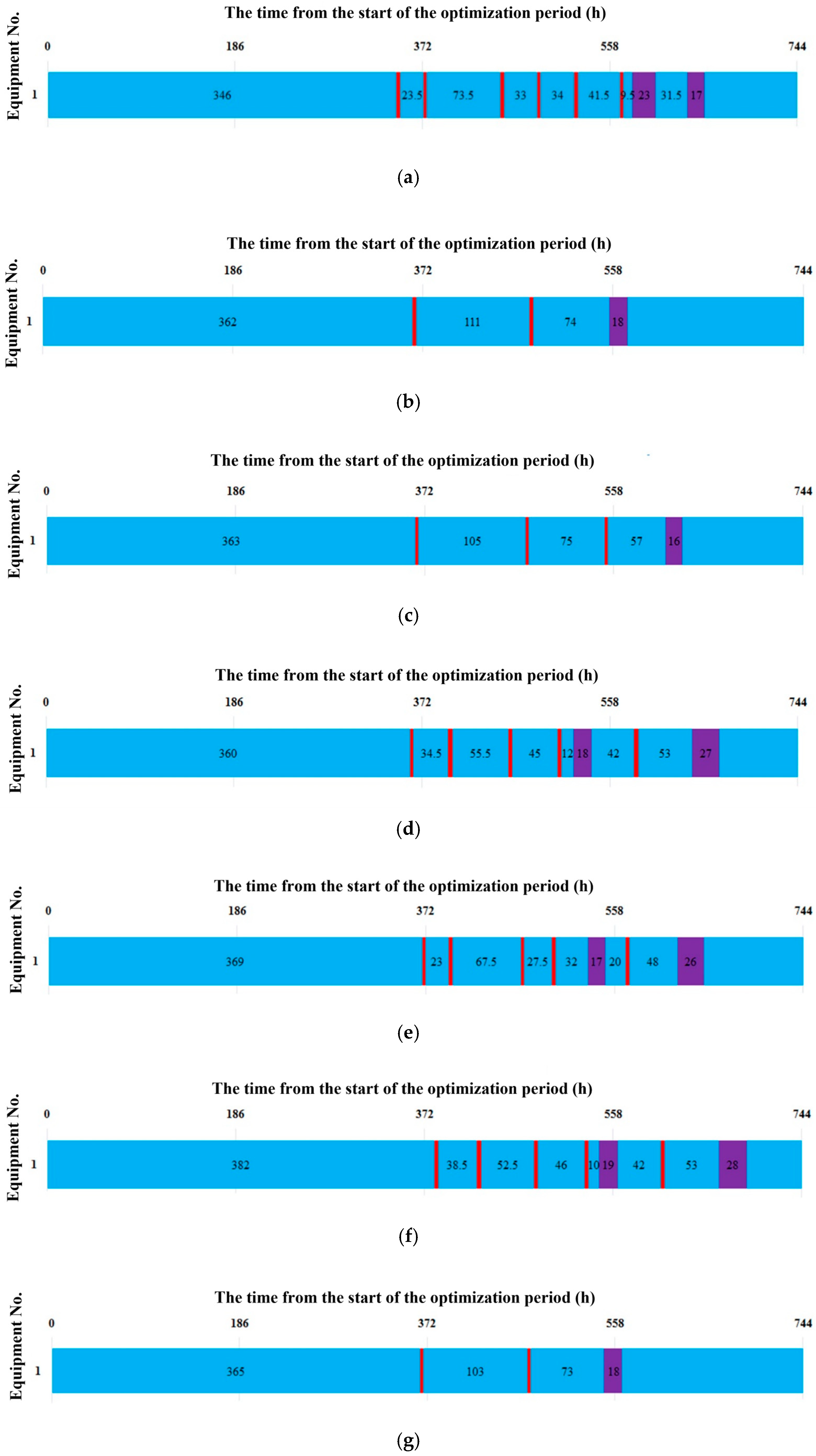
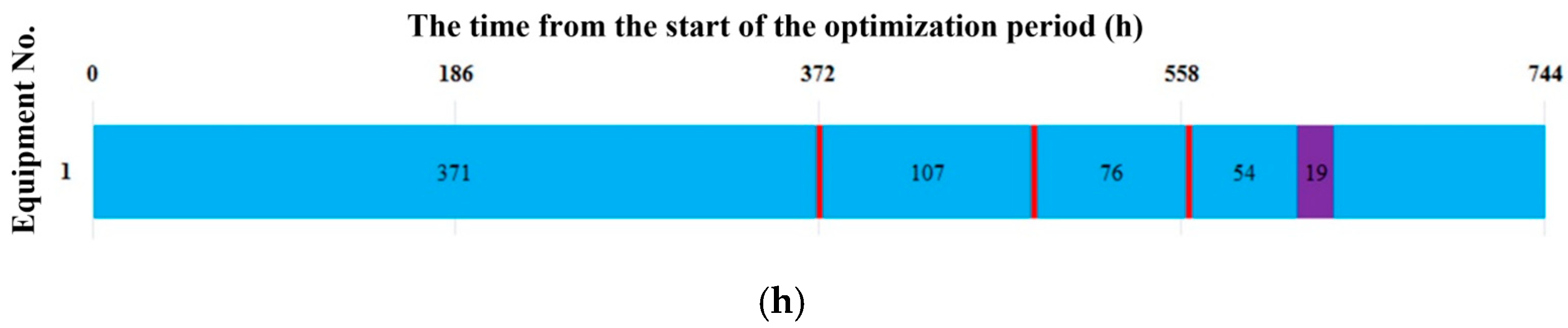
4.2.1. Initial Maintenance Optimization Scheme

According to historical data, values of γ i β i and a i in the failure rate evolution function are first fitted, and the duration of PdM and minimal repair are determined, whose results are shown in Table 8. After that, the H i 0 , N i , and T i j for equipment i can be determined, as shown in Table 9 and Table 10. ( T i P l e a d , T i P l a g ) can thus be obtained. Next, the equipment-level and initial flow-level maintenance optimization scheme for operation lines can be obtained by our proposed method.
The equipment-level maintenance timetables of reclaiming operation line u1 (BQ3–R5) and u2 (R6(R7)–BQ4) are shown in Figure 5a,b, where the blue section indicates normal operation of handling equipment, the red section indicates minimal repair, and the purple section indicates PdM. Since the adjustment of the lower-priority BQ3 within its PdMI threshold does not enable it to take advantage of the maintenance opportunities provided by the higher-priority R5, the maintenance interval of u1 is the union of the maintenance intervals for BQ3 and R5, whose initial flow-level maintenance timetable is shown in Figure 6a. Since R6 and R7 are in parallel, while the intersection of their actual shutdown interval can be an empty set by adjusting the PdMIL of lower-priority equipment R7, they can be equivalent to a piece of handling equipment running all the time, whose impact on the handling equipment BQ4 can be neglected. Therefore, the initial flow-level maintenance timetable of u2 is the same as the equipment-level maintenance timetable of BQ4 (shown in Figure 6b). Similarly, the initial flow-level maintenance timetables of u3, w1, w2, w3, v1, and v2 are shown in Figure 6c–h.

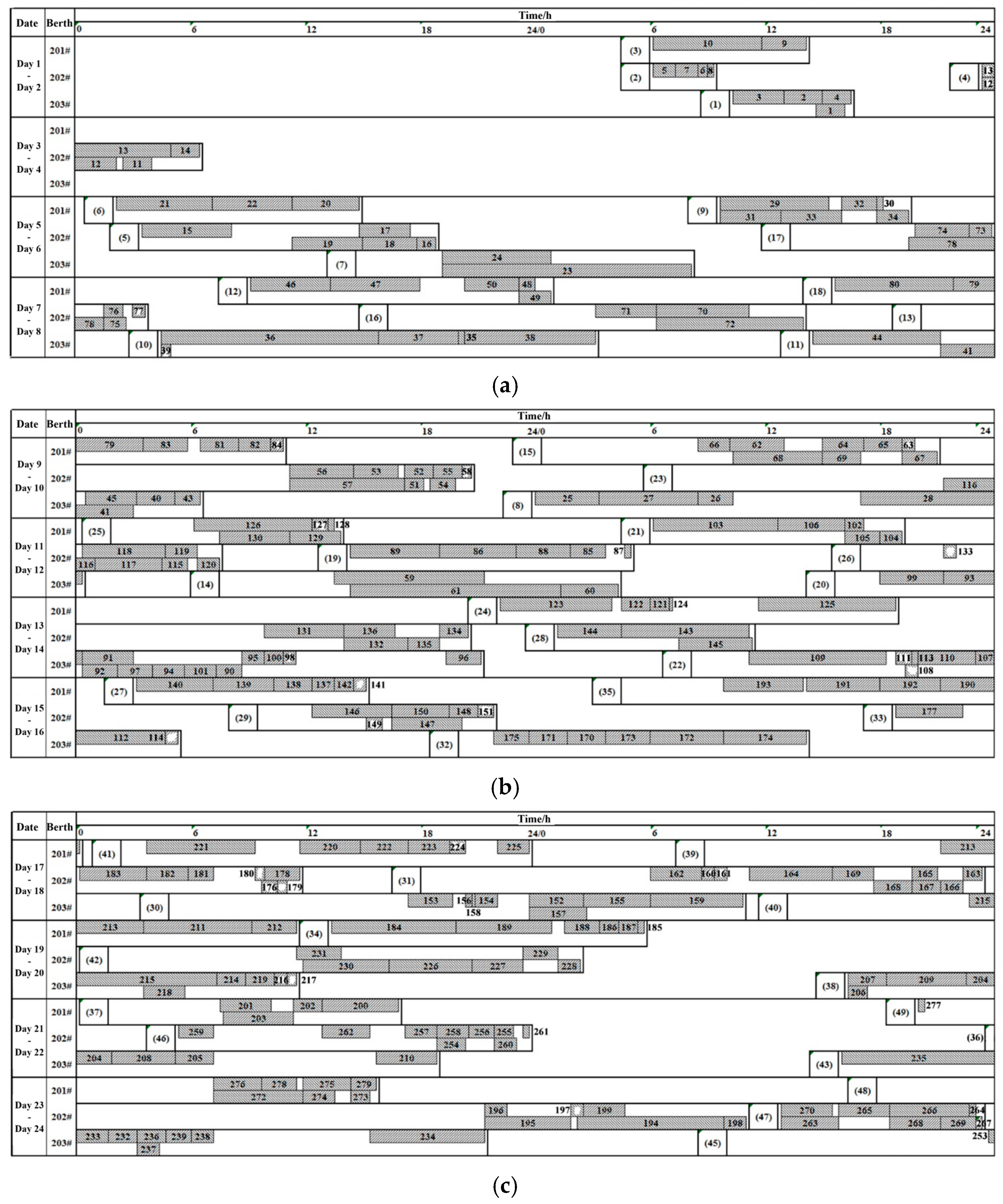
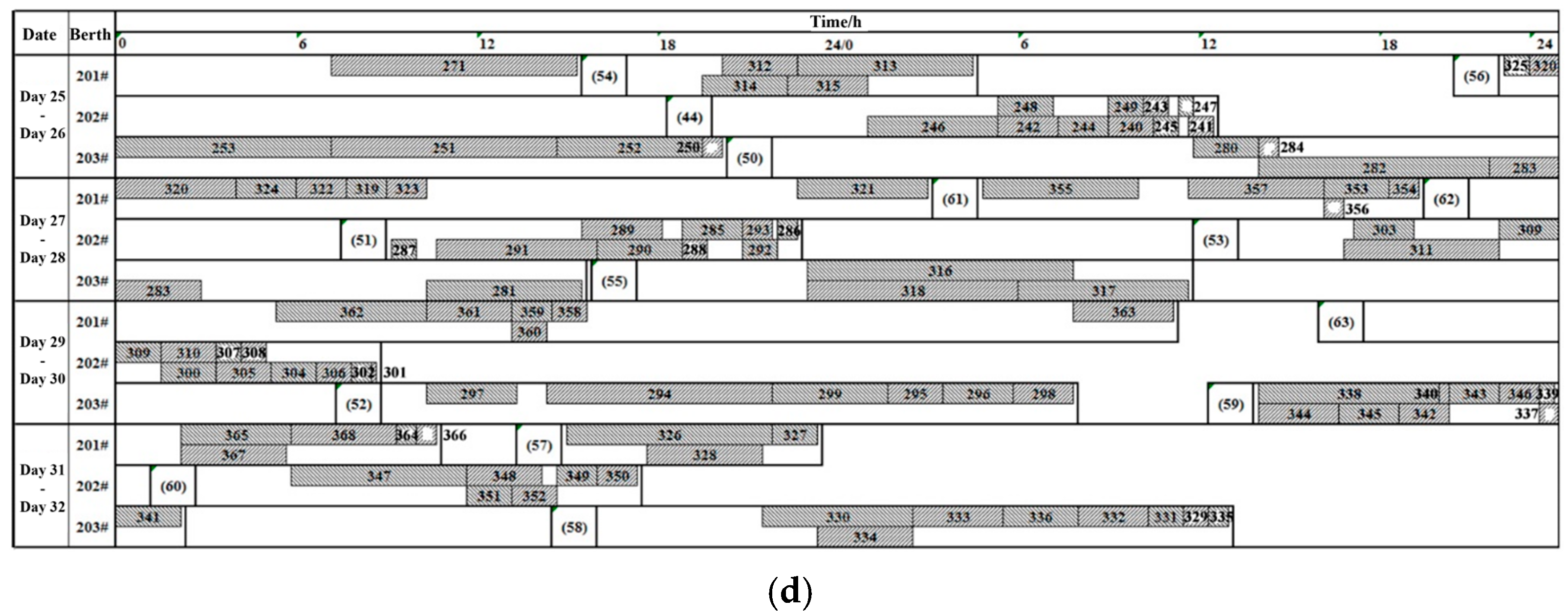
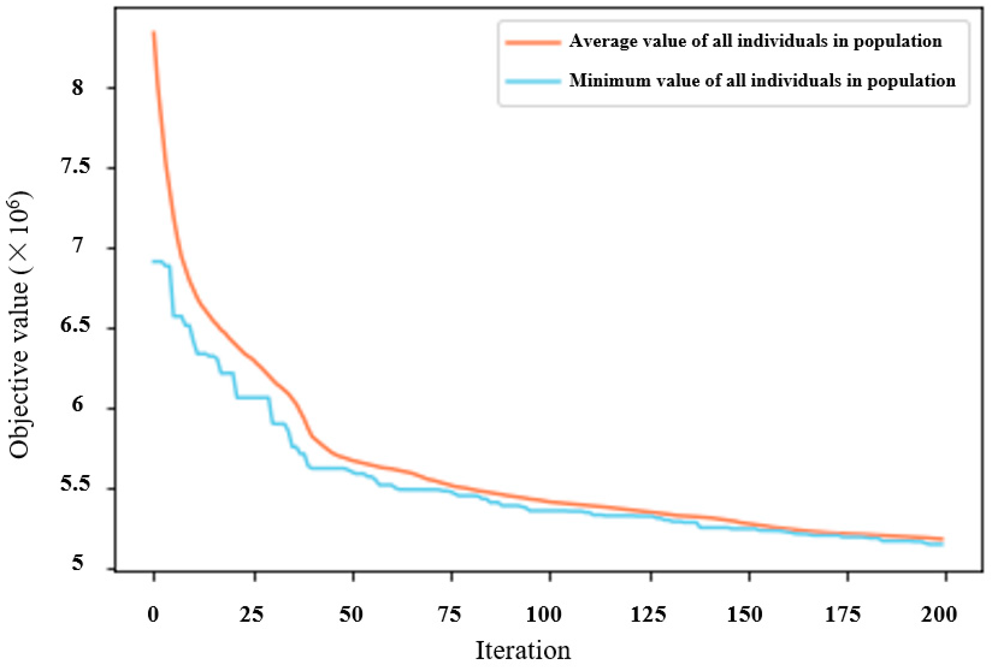
4.2.2. Scheduling Optimization Considering Maintenance

The basic parameters of the genetic algorithm are shown in Table 11. The two-layer algorithm is used to solve the scheduling optimization problem considering maintenance, and the ship scheduling scheme of the optimal solution is shown in Figure 7a–d. It can be seen from the calculation process diagram of the genetic algorithm (see Figure 8) that the algorithm has good convergence.
By comparing the optimal solution with the actual schedule of the terminal (see Table 12), it can be seen that the proposed method in this study can effectively reduce C t i m e by 15.0% and C m a i n t e n a n c e by 77.4%. On the one hand, the “equipment-level–flow-level” maintenance method reduces unnecessary equipment maintenance. On the other hand, the use of OM strategy, together with suitable scheduling of operation lines, decreases the effect of equipment maintenance on ship-loading operation, and reduces the average dwell time of a ship at terminal by 15.8% from 23.4 h to 19.7 h. For C e n e r g y , since the start-up energy cost is relatively small compared with the transportation energy cost, while the transportation energy cost is almost fixed once the ship-loading operation task is determined, C e n e r g y can only be saved by 0.3%. Overall, the total cost of maintenance and scheduling for the ship-loading operation system in the coal export terminal C t o t a l can be saved by 10.3%, which verifies the effectiveness of the proposed method.
Furthermore, we employed the method in Gan et al. [47] and Abdollahzadeh-Sangroudi et al. [48] to solve the scheduling optimization problem of the ship-loading operation system considering equipment maintenance, and the comparison of optimal solutions by different methods is listed in Table 13.
From the table, we can see that although Gan et al. [47] also used GA, the OM-based “equipment-level–flow-level” maintenance optimization in this paper shows its superiority, obtaining lower C t i m e and C m a i n t e n a n c e due to a better equipment maintenance scheme. As for the method in Abdollahzadeh-Sangroudi et al. [48], it can obtain the same optimal equipment maintenance scheme. However, compared with the Cuckoo Optimization Algorithm, GA with specific population initialization and genetic operator in this paper are more suitable for a ship-loading operation system, as it can obtain lower C t i m e .
Furthermore, we can find that better equipment maintenance schemes not only reduce unnecessary equipment maintenance time and cost but also effectively save the waiting time of ships at terminal caused by equipment failure and maintenance, leading to higher handling operation efficiency and lower operation cost of the coal export terminal.

5. Conclusions and Future Work

As important nodes of the global coal supply chain, coal export terminals meet with challenges including poor working conditions of the handling equipment and relatively fixed layout, such that frequent equipment failures seriously affect the efficiency and stability of ship-loading operations. To solve the problem, in this study, a scheduling optimization model for the ship-loading operation system in the coal export terminal considering equipment maintenance is established. To deal with the complicated interaction between scheduling and maintenance of the system, the concept of opportunity maintenance is introduced and a two-layer algorithm is proposed. The actual operation and maintenance data of a coal export terminal in China are taken as an example to verify the effectiveness of the proposed method, and the results show that the average dwell time reduction and total cost saving reach 15.8% and 10.3%, respectively. A comparison of the proposed method and the opportunity-maintenance-based scheduling method in existing studies is also presented.
To our knowledge, this is the first work that considers the effect of equipment maintenance on handling operation scheduling in coal export terminals. This study expresses how to deal with equipment maintenance in scheduling problems of port systems through actual operation and maintenance data. The proposed method can effectively reduce unnecessary equipment maintenance and decrease the waiting time of ships at terminal caused by equipment maintenance, which can provide ship-loading operation system scheduling plans for port managers, as well as equipment maintenance plans for equipment maintenance workers.
One of the main limitations of this paper lies in that the arranged berth of the ship arriving at the terminal is assumed to be known. In the future, the joint optimization of berth allocation and ship-loading operation system scheduling with the consideration of equipment maintenance may be another topic worth exploring.

Author Contributions

Conceptualization, Q.T. and W.W.; methodology, Q.T.; software, Q.T.; validation, X.X.; formal analysis, Y.P.; investigation, Q.T. and Y.P.; resources, X.X.; data curation, W.W.; writing—original draft preparation, Q.T.; writing—review and editing, Y.P.; visualization, X.X.; supervision, Y.P.; project administration, W.W.; funding acquisition, Q.T. All authors have read and agreed to the published version of the manuscript.

Funding

This research was funded by the National Key R&D Program of China (Grant No. 2022YFB2602300) the National Natural Science Foundation of China (Grant No. 52272318), and the Natural Science Foundation of Liaoning Province (Grant No. 2023-BSBA-045).

Institutional Review Board Statement

Not applicable.

Informed Consent Statement

Not applicable.

Data Availability Statement

The original contributions presented in the study are included in the article, further inquiries can be directed to the corresponding author.

Conflicts of Interest

The authors declare no conflict of interest.

References

  1. Ouhaman, A.A.; Benjelloun, K.; Kenné, J.P.; Najid, N. The storage space allocation problem in a dry bulk terminal: A heuristic solution. IFAC-PapersOnLine 2020, 53, 10822–10827. [Google Scholar] [CrossRef]
  2. Xin, J.; Negenborn, R.R.; van Vianen, T. A hybrid dynamical approach for allocating materials in a dry bulk terminal. IEEE Trans. Autom. Sci. Eng. 2018, 15, 1326–1336. [Google Scholar] [CrossRef]
  3. Savelsbergh, M.; Smith, O. Cargo assembly planning. EURO J. Transp. Logist. 2015, 4, 321–354. [Google Scholar] [CrossRef]
  4. Burdett, R.L.; Corry, P.; Eustace, C. Stockpile scheduling with geometry constraints in dry bulk terminals. Comput. Oper. Res. 2021, 130, 105224. [Google Scholar] [CrossRef]
  5. Angelelli, E.; Kalinowski, T.; Kapoor, R.; Savelsbergh, M.W.P. A reclaimer scheduling problem arising in coal stockyard management. J. Sched. 2015, 19, 563–582. [Google Scholar] [CrossRef]
  6. Kalinowski, T.; Kapoor, R.; Savelsbergh, M.W.P. Scheduling reclaimers serving a stock pad at a coal terminal. J. Sched. 2017, 20, 85–101. [Google Scholar] [CrossRef]
  7. Belassiria, I.; Mazouzi, M.; Elfezazi, S.; Torbi, I. A heuristic methods for stacker and reclaimer scheduling problem in coal storage area. In Proceedings of the 2019 International Colloquium on Logistics and Supply Chain Management (LOGISTIQUA), Paris, France, 12–14 June 2019; IEEE: New York, NY, USA; pp. 1–7. [Google Scholar]
  8. van Vianen, T.; Ottjes, J.; Lodewijks, G. Simulation-based rescheduling of the stacker–reclaimer operation. J. Comput. Sci. 2015, 10, 149–154. [Google Scholar] [CrossRef]
  9. Hu, D.; Yao, Z. Stacker-reclaimer scheduling in a dry bulk terminal. Int. J. Comput. Integr. Manuf. 2012, 25, 1047–1058. [Google Scholar] [CrossRef]
  10. Ünsal, O. Reclaimer scheduling in dry bulk terminals. IEEE Access 2020, 8, 96294–96303. [Google Scholar] [CrossRef]
  11. Ernst, A.T.; Oğuz, C.; Singh, G.; Taherkhani, G. Mathematical models for the berth allocation problem in dry bulk terminals. J. Sched. 2017, 20, 459–473. [Google Scholar] [CrossRef]
  12. Cheimanoff, N.; Fontane, F.; Kitri, M.N.; Tchernev, N. A reduced VNS based approach for the dynamic continuous berth allocation problem in bulk terminals with tidal constraints. Expert Syst. Appl. 2021, 168, 114215. [Google Scholar] [CrossRef]
  13. de León, A.D.; Lalla-Ruiz, E.; Melián-Batista, B.; Moreno-Vega, J.M. A Machine Learning-based system for berth scheduling at bulk terminals. Expert Syst. Appl. 2017, 87, 170–182. [Google Scholar] [CrossRef]
  14. Hu, X.N.; Yan, W.; He, J.L.; Bian, Z.C. Study on Bulk Terminal Berth Allocation Based on Heuristic Algorithm. In Proceedings of the 2012 International Conference of Modern Computer Science and Applications, Wuhan, China, 8 September 2012; Springer: Berlin/Heidelberg, Germany, 2013; pp. 413–419. [Google Scholar]
  15. Guo, Z.; Cao, Z.; Wang, W.; Jiang, Y.; Xu, X.; Feng, P. An integrated model for vessel traffic and deballasting scheduling in coal export terminals. Transp. Res. Part E Logist. Transp. Rev. 2021, 152, 102409. [Google Scholar] [CrossRef]
  16. Burdett, R.L.; Corry, P.; Eustace, C.; Smith, S. A flexible job shop scheduling approach with operators for coal export terminals—A mature approach. Comput. Oper. Res. 2020, 115, 104834. [Google Scholar] [CrossRef]
  17. Belov, G.; Boland, N.L.; Savelsbergh, M.W.P.; Stuckey, P.J. Logistics optimization for a coal supply chain. J. Heuristics 2020, 26, 269–300. [Google Scholar] [CrossRef]
  18. Burdett, R.L.; Corry, P.; Yarlagadda, P.K.; Eustace, C.; Smith, S. A flexible job shop scheduling approach with operators for coal export terminals. Comput. Oper. Res. 2019, 104, 15–36. [Google Scholar] [CrossRef]
  19. de Andrade, J.L.M.D.; Menezes, G.C. An Integrated Planning, Scheduling, Yard Allocation and Berth Allocation Problem in Bulk Ports: Model and Heuristics. In Proceedings of the International Conference on Computational Logistics, Enschede, The Netherlands, 27–29 September 2021; Springer: Cham, Switzerland, 2021; pp. 3–20. [Google Scholar]
  20. Unsal, O.; Oguz, C. An exact algorithm for integrated planning of operations in dry bulk terminals. Transp. Res. Part E Logist. Transp. Rev. 2019, 126, 103–121. [Google Scholar] [CrossRef]
  21. Menezes, G.C.; Mateus, G.R.; Ravetti, M.G. A hierarchical approach to solve a production planning and scheduling problem in bulk cargo terminal. Comput. Ind. Eng. 2016, 97, 1–14. [Google Scholar] [CrossRef]
  22. Jiang, X.; Zhong, M.; Shi, J.; Li, W. Optimization of integrated scheduling of restricted channels, berths, and yards in bulk cargo ports considering carbon emissions. Expert Syst. Appl. 2024, 255, 124604. [Google Scholar] [CrossRef]
  23. Balakrishnan, S.; Lim, T.; Zhang, Z. A methodology for evaluating the economic risks of hurricane-related disruptions to port operations. Transp. Res. Part A Policy Pract. 2022, 162, 58–79. [Google Scholar] [CrossRef]
  24. Lewandowski, M.; Scholz-Reiter, B. A framework for systematic design and operation of condition-based maintenance systems: Evidence from a case study of fleet management at sea ports. Int. J. Ind. Eng. Theory Appl. Pract. 2013, 20, 2–11. [Google Scholar]
  25. Widarto, H.; Handani, D.W. Maintenance scheduling for Diesel Generator support system of Container Crane using system dynamic modeling. In Proceedings of the 2015 International Conference on Advanced Mechatronics, Intelligent Manufacture, and Industrial Automation (ICAMIMIA), Surabaya, Indonesia, 15–16 October 2015; IEEE: New York, NY, USA; pp. 188–193. [Google Scholar]
  26. Mhalla, A.; Zhang, H.; Dutilleul, S.C.; Benrejeb, M. Age-dependent maintenance planning based on P-time Petri Nets for Seaport equipment. In Proceedings of the Engineering and Technology (PET), Hammamet, Tunisia, 22–25 March 2016; pp. 76–82. [Google Scholar]
  27. Szpytko, J.; Duarte, Y.S. Digital twins model for cranes operating in container terminal. IFAC-PapersOnLine 2019, 52, 25–30. [Google Scholar] [CrossRef]
  28. Lin, D.; Jin, B.; Chang, D. A PSO approach for the integrated maintenance model. Reliab. Eng. Syst. Saf. 2020, 193, 106625. [Google Scholar] [CrossRef]
  29. Tchotang, T.; Meva’a, L.; Kenmeugne, B.; Jatta, P.V. Reliability analysis of a reach stacker in relation to repair maintenance cost and time: A case study of the Gambia sea port. Life Cycle Reliab. Saf. Eng. 2020, 9, 283–289. [Google Scholar] [CrossRef]
  30. Zheng, F.; Li, Y.; Chu, F.; Liu, M.; Xu, Y. Integrated berth allocation and quay crane assignment with maintenance activities. Int. J. Prod. Res. 2019, 57, 3478–3503. [Google Scholar] [CrossRef]
  31. Krimi, I.; Todosijević, R.; Benmansour, R.; Ratli, M.; El Cadi, A.A.; Aloullal, A. Modelling and solving the multi-quays berth allocation and crane assignment problem with availability constraints. J. Glob. Optim. 2020, 78, 349–373. [Google Scholar] [CrossRef]
  32. Sepehri, A.; Kirichek, A.; van der Werff, S.; Baart, F.; van den Heuvel, M.; van Koningsveld, M. Analyzing the interac-tion between maintenance dredging and seagoing vessels: A case study in the Port of Rotterdam. J. Soils Sediments 2024, 1–11. [Google Scholar] [CrossRef]
  33. Lu, Y.; Wang, S.; Zhang, C.; Chen, R.; Dui, H.; Mu, R. Adaptive maintenance window-based opportunistic mainte-nance optimization considering operational reliability and cost. Reliab. Eng. Syst. Saf. 2024, 250, 110292. [Google Scholar] [CrossRef]
  34. Huang, M.; Qi, F.; Wang, L. Novel condition-based opportunistic maintenance policy for series systems with de-pendent competing failure processes. Proc. Inst. Mech. Eng. Part O J. Risk Reliab. 2024. [Google Scholar] [CrossRef]
  35. Li, M.; Wu, B. Optimal condition-based opportunistic maintenance policy for two-component systems considering common cause failure. Reliab. Eng. Syst. Saf. 2024, 250, 110269. [Google Scholar] [CrossRef]
  36. Su, H.; Cao, Q.; Li, Y. Condition-based opportunistic maintenance strategy for multi-component wind turbines by using stochastic differential equations. Sci. Rep. 2024, 14, 1–15. [Google Scholar] [CrossRef] [PubMed]
  37. Chen, W.; Sun, C.; Pei, T.; Li, M.; Lei, H. Opportunistic maintenance strategies for PV power systems considering the structural correlation. Electr. Eng. 2024, 1–13. [Google Scholar] [CrossRef]
  38. Wang, J.; Xia, Y.; Qin, Y.; Zhang, X. Optimal external opportunistic maintenance for wind turbines considering wind speed. Int. J. Green Energy 2024, 21, 2022–2041. [Google Scholar] [CrossRef]
  39. Chen, Z.; Chen, Z.; Zhou, D.; Xia, T.; Pan, E. Opportunistic maintenance optimization of continuous process manu-facturing systems considering imperfect maintenance with epistemic uncertainty. J. Manuf. Syst. 2023, 71, 406–420. [Google Scholar] [CrossRef]
  40. Dinh, D.-H.; Do, P.; Bang, T.Q.; Nguyen-Ho, S.-H. Degradation modeling and opportunistic maintenance for two-component systems with an intermittent operation component. Comput. Ind. Eng. 2023, 185, 109698. [Google Scholar] [CrossRef]
  41. Dinh, D.-H.; Do, P.; Iung, B.; Nguyen, P.-T. Reliability modeling and opportunistic maintenance optimization for a multicomponent system with structural dependence. Reliab. Eng. Syst. Saf. 2024, 241, 109708. [Google Scholar] [CrossRef]
  42. Li, X.; Ran, Y.; Chen, B.; Chen, F.; Cai, Y.; Zhang, G. Opportunistic maintenance strategy optimization considering imperfect maintenance under hybrid unit-level maintenance strategy. Comput. Ind. Eng. 2023, 185, 109624. [Google Scholar] [CrossRef]
  43. Wei, F.; Wang, J.; Ma, X.; Yang, L.; Qiu, Q. An Optimal Opportunistic Maintenance Planning Integrating Discrete- and Continuous-State Information. Mathematics 2023, 11, 3322. [Google Scholar] [CrossRef]
  44. Chen, W.; Li, M.; Pei, T.; Sun, C. Research on opportunity maintenance strategy for PV power generation systems considering random impact. Electr. Eng. 2024, 1–12. [Google Scholar] [CrossRef]
  45. Li, J.; Wang, H.; Xiong, L.; He, Y.; Yi, C. Strategy Optimization of Multi-component System Opportunity Maintenance for Electric Multiple Units from a Lean Maintenance Perspective. IEEE Access 2023, 11, 89478–89487. [Google Scholar] [CrossRef]
  46. Yuan, Q.; Jin, Z.; Jia, S.; Liu, Q. An improved opportunity maintenance model of complex system. Adv. Mech. Eng. 2019, 11, 1687814019841517. [Google Scholar] [CrossRef]
  47. Gan, J.; Zhang, W.; Wang, S.; Zhang, X. Joint decision of condition-based opportunistic maintenance and scheduling for multi-component production systems. Int. J. Prod. Res. 2022, 60, 5155–5175. [Google Scholar] [CrossRef]
  48. Abdollahzadeh-Sangroudi, H.; Moazzam-Jazi, E.; Tavakkoli-Moghaddam, R.; Ranjbar-Bourani, M. Dynamic oppor-tunistic maintenance grouping in a lot streaming based job-shop scheduling problem. Comput. Ind. Eng. 2023, 183, 109424. [Google Scholar] [CrossRef]
Figure 1. A sketch of the ship-loading operation flow in a dry bulk port.
Jmse 12 01377 g001
Figure 2. OM-based two-layer algorithm.
Jmse 12 01377 g002
Figure 3. “Equipment-level–flow-level” maintenance optimization method.
Jmse 12 01377 g003
Figure 4. Ship-loading operation system layout for the terminal.
Jmse 12 01377 g004
Figure 5. Equipment-level maintenance timetable of operation lines (a) u1; (b) u2.
Jmse 12 01377 g005
Figure 6. Initial flow-level maintenance timetables of operation lines (a) u1; (b) u2; (c) u3; (d) w1; (e) w2; (f) w3; (g) v1; and (h) v2.
Jmse 12 01377 g006aJmse 12 01377 g006b
Figure 7. Ship scheduling scheme of the optimal solution: (a) Day 1 to Day 8; (b) Day 9 to Day 16; (c) Day 17 to Day 24; (d) Day 25 to Day 32.
Jmse 12 01377 g007aJmse 12 01377 g007b
Figure 8. Genetic algorithm calculation process diagram.
Jmse 12 01377 g008
Table 1. Notations and descriptions.
NotationDescription
Sets and indices
SSet of ships arriving at the terminal, s 1 , , S
USet of reclaiming operation line, u 1 , , U
VSet of horizontal operation line, v 1 , , V
WSet of ship-loading operation line, w 1 , , W
MSet of ship-loading task, m 1 , , M
I m Set of handling equipment used by task m, i 1 , , I m
N i m Set of PdM for equipment i during task m, j 1 , , N i m
KSet of berth, k 1 , , K
TSet of time, t 0 , , T
PSet of pile, p 1 , , P
Parameters
C t o t a l Total cost of maintenance and scheduling for ship-loading operation system in coal export terminal
C t i m e Dwell time cost of ships at the terminal
C e n e r g y Energy consumption cost of operation lines
C m a i n t e n a n c e Handling equipment maintenance cost
t s a r r , s S Time of ship arriving at the terminal
t s d e p , s S Time of ship leaving the terminal
E s s h , s S Dwell time cost of ship s at port per unit time
E u b q , u U Energy cost of transporting unit coal for reclaiming operation line u
E v b c , v V Energy cost of transporting unit coal for horizontal operation line v
E w b m , w W Energy cost of transporting unit coal for ship-loading operation line w
d m , m M Coal required by task m
A u b q , u U Start-up energy cost each time for reclaiming operation line u
A v b c , v V Start-up energy cost each time for horizontal operation line v
A w b m , w W Start-up energy cost each time for ship-loading operation line w
a m , u b q , m M , u U Number of start-ups for reclaiming operation line u to finish task m
a m , v b c , m M , v V Number of start-ups for horizontal operation line v to finish task m
a m , w b m , m M , w W Number of start-ups for ship-loading operation line w to finish task m
E i s m , i I m Maintenance cost of each PdM for equipment i
N i m j , i I m , m M , j N i m Number of minimal repairs for equipment i in its jth PdMI during ship-loading task m
E i m j u m , i I m , m M , j N i m Maintenance cost of each minimal repair for equipment i in its jth PdMI during ship-loading task m
M Large positive constant
t m s Start time of task m
τ m t a Operation duration of task m
τ m d o w n Maintenance duration of task m
τ s u n Unmoor duration of ship s
τ s a u x Auxiliary operation duration of ship s
φ m , m Operation time interval between task m and m’
π k , k Duration of the ship-loader moving from berth k to berth k’
η Operation time interval of two tasks that belong to the same berth and occupy two ship-loaders next to the berth respectively
Variables
Decision variables
y m , u b q 0 , 1 , m M , u U 1 if reclaiming operation line u is occupied by task m, 0 otherwise
y m , v b c 0 , 1 , m M , v V 1 if horizontal operation line v is occupied by task m, 0 otherwise
y m , w b m 0 , 1 , m M , w W 1 if ship-loading operation line w is occupied by task m, 0 otherwise
z s , s s h 0 , 1 , s , s S 1 if priority of ship s is higher than that of ship s’, 0 otherwise
z m , m t a 0 , 1 , m , m M 1 if priority of task m is higher than that of task m’, 0 otherwise
T i m j , i I m , m M , j N i m PdMIL for equipment i in its jth PdMI during task m
Auxiliary variables
β s , k 0 , 1 , s S , k K 1 if ship s is arranged to berth k, 0 otherwise
θ s , m 0 , 1 , s S , m M 1 if task m belongs to ship s, 0 otherwise
γ m , p 0 , 1 , m M , p P 1 if pile p is selected to unload coal by task m, 0 otherwise
ε m , m 0 , 1 , m , m M 1 if task m and m’ belong to the ship berthing at the same berth and occupy two ship-loaders next to the berth respectively, 0 otherwise
δ m , k 0 , 1 , m M , k K 1 if task m belongs to the ship berthing at berth k, 0 otherwise
x m , t t a 0 , 1 , m M , t T 1 if task m is in process at time t, 0 otherwise
Table 2. The chromosome coding structure.
SequenceLengthBerth 1Berth 2Berth m
Berthing priority of shipm b 1 b 2 b m
Priority of ship-loading taskn c 1 , c 2 , c n 1 c n 1 + 1 , c n 1 + 2 , c n 2 c n m 1 + 1 , c n m 1 + 2 , c n
Reclaiming operation linen e 1 , e 2 , e n 1 e n 1 + 1 , e n 1 + 2 , e n 2 e n m 1 + 1 , e n m 1 + 2 , e n
Horizontal operation linen f 1 , f 2 , f n 1 f n 1 + 1 , f n 1 + 2 , f n 2 f n m 1 + 1 , f n m 1 + 2 , f n
Ship-loading operation linen g 1 , g 2 , g n 1 g n 1 + 1 , g n 1 + 2 , g n 2 g n m 1 + 1 , g n m 1 + 2 , g n
Table 3. OM procedure for ship-loading operation flow.
Step 1. Calculate each PdMIL threshold for equipment i in the flow, T i P l e a d , T i P l a g ,   i 1 , 2 , , I ,   P 1 , 2 , , N i , where I is the total number of pieces of equipment in the flow and N i is the total number of PdMIs in life cycle of equipment i.
Step 2. Judge whether equipment i is in parallel with other handling equipment. If so, go to Step 4; otherwise, rank the priority of equipment in parallel part according to the duration of PdM T i s m . The larger the T i s m , the higher the priority (the smaller the priority number).
Step 3. When i < N p i , where N p i is the total number of pieces of equipment in parallel part, repeat the step as follows, otherwise go to Step 4.
Step 3.1. Determine equipment i’s shutdown interval caused by PdM t i j s m s , t i j s m f and minimal repair t i j k u m s , t i j k u m s + τ i j k u m , to determine its actual shutdown interval t i d o w n s , t i d o w n f .
Step 3.2. Determine the initial shutdown interval of equipment m = i + 1 caused by PdM t m n s m s , t m n s m f and minimal repair t m n p u m s , t m n p u m s + t o , to determine its actual shutdown interval t m d o w n s , t m d o w n f .
Step 3.3. When no matter how adjusted T m n T m n l e a d , T m n l a g , t i d o w n s , t i d o w n f t m d o w n s , t m d o w n f cannot be an empty set, treat equipment i and m as equipment i with actual shutdown interval t i d o w n s , t i d o w n f = m i n t i d o w n s , t i d o w n f t m d o w n s , t m d o w n f , set priority of equipment i as lowest, and consider its effect on availability of the ship-loading operation flow. Otherwise, treat equipment i and m as equipment i which is always working, and it is unnecessary to consider the series-parallel relationship with other handling equipment.
Step 3.4. Consider the maintenance opportunities provided by equipment i and equipment m, and determine the next equipment.
Step 4. Rank the priority of equipment in serial part according to the duration of PdM T i s m . The larger the T i s m , the higher the priority (the smaller the priority number).
Step 5. When i < N s i , where N s i is the total number of pieces of equipment in serial parts, repeat the step as follows, otherwise go to Step 6.
Step 5.1. Determine equipment i’s shutdown interval caused by PdM t i j s m s , t i j s m f and minimal repair t i j k u m s , t i j k u m s + τ i j k u m , to determine its actual shutdown interval t i d o w n s , t i d o w n f .
Step 5.2. Determine the initial shutdown interval of equipment m = i + 1 caused by PdM t m n s m s , t m n s m f and minimal repair t m n p u m s , t m n p u m s + τ m n p u m , to determine its actual shutdown interval t m d o w n s , t m d o w n f .
Step 5.3. Maximize t m n s m s , t m n s m f t i j s m s , t i j s m f by adjusting T m n T m n l e a d , T m n l a g according to t i j s m s , t i j s m f .
Step 5.4. Consider the maintenance opportunities provided by equipment i and equipment m, and determine the next equipment.
Step 6. Consider the effect of parallel parts, and calculate the availability of the whole ship-loading operation flow E T A F by Equations (52) and (53).
Table 4. Relationship between operating line, handling equipment, and pile.
Operation LineNo.Equipment 1Equipment 2Pile
Reclaiming operation line u1BQ3R5P01–P08
2BQ4R6(R7)P09–P24
3BQ5R8(R9)P25–P40
Horizontal operation line v1BC3-
2BC4-
Ship-loading operation line w1BM4SL4
2BM5SL5
3BM6SL6
Table 5. Accessibility of operating line.
BerthReclaiming Operation Line uHorizontal Operation Line vShip-Loading Operation Line w
201#1-1
211
311
202#212
312
222
322
203#1-3
223
323
Table 6. Basic information on ship arrivals.
Ship’s No.Arrival DateArrival TimeBerthTask No.Unit Dwell Time Cost of Ship (CNY/h)
12 January 20179:49203#1–41416
22 January 20175:40202#5–81416
32 January 20175:38201#9–101416
42 January 201722:50202#11–141416
55 January 20172:56202#15–191416
65 January 20171:44201#20–221416
75 January 201714:23203#23–241416
89 January 201723:33203#25–281416
96 January 20179:07201#29–341416
107 January 20173:56203#35–391416
118 January 201714:02203#40–451416
127 January 20178:43201#46–501416
138 January 201719:46202#51–581416
1411 January 20177:10203#59–611416
1510 January 20170:00201#62–691416
167 January 201715:58202#70–721416
176 January 201713:04202#73–781416
188 January 201715:11201#79–841416
1911 January 201713:52202#85–891416
2012 January 201715:15203#90–1011592
2112 January 20175:36201#102–1061416
2214 January 20177:46203#107–1141416
2310 January 20176:50202#115–1201416
2413 January 201721:43201#121–1251416
2511 January 20171:26201#126–1301416
2612 January 201716:42202#131–1361416
2715 January 20172:36201#137–1421416
2814 January 20170:39202#143–1451416
2915 January 20179:11202#146–1511416
3017 January 20174:34203#152–1591416
3117 January 201717:43202#160–1691592
3215 January 201719:40203#170–1751416
3316 January 201718:16202#176–1831592
3419 January 20176:37201#184–1891416
3516 January 20174:09201#190–1931416
3623 January 20170:41202#194–1991416
3721 January 20171:17201#200–2031416
3820 January 201715:51203#204–2101416
3918 January 20178:27201#211–2131416
4018 January 201712:50203#214–2191416
4117 January 20172:02201#220–2251416
4219 January 20171:15202#226–2311416
4322 January 201715:32203#232–2391416
4425 January 201719:29202#240–2491592
4524 January 20179:38203#250–2531416
4621 January 20174:48202#254–2621592
4724 January 20174:03202#263–2701416
4824 January 201717:26201#271–2711416
4922 January 201719:28201#272–2791416
5025 January 201720:36203#280–2841416
5127 January 20178:40202#285–2931592
5229 January 20178:28203#294–2991416
5328 January 201713:01202#300–3111592
5425 January 201713:28201#312–3151416
5527 January 201716:59203#316–3181416
5626 January 201721:43201#319–3251416
5731 January 201714:27201#326–3281416
5831 January 201715:44203#329–3361416
5930 January 201713:27203#337–3461416
6031 January 20172:15202#347–3521416
6128 January 20170:52201#353–3571416
6228 January 201719:34201#358–3631416
6330 January 201717:11201#364–3681592
Table 7. Unit cost of maintenance and unit energy consumption cost.
Operation LineUnit Cost of PdM
(Thousand CNY)
Unit Cost of Minimal Repair
(Thousand CNY)
Transportation Cost per Ton
(CNY)
Start-Up Cost Each Time
(CNY)
u178180.49102
u272190.63130
u385160.63130
v152100.085.2
v25590.085.2
w1124200.3961
w2117230.3991
w3130260.39123
Table 8. Fitting results of failure rate evolution function parameters, PdM duration, and minimal repair duration of equipment.
Serial No. iEquipment γ i β i a i T i s m (h) τ i j u m (h)
1BQ31.030.011173
2BQ41.060.010183.5
3BQ51.020.025163
4R51.030.089233.5
5R61.040.018254
6R71.020.060243.5
7R81.030.018243.5
8R91.040.088233
9BC31.040.126183
10BC41.020.090193
11BM41.060.019183.5
12BM51.030.018173
13BM61.040.020193.5
14SL41.020.069274
15SL51.030.070263.5
16SL61.040.066284
Table 9. H i 0 , N i , and T i j for equipment i.
iEquipment H i 0 N i T i 1 T i 2 T i 3 T i 4 T i 5 T i 6 T i 7 T i 8 T i 9 T i 10 T i 11 T i 12
1BQ30.8726626 609 592 575 559 544 529 514 500 486 473 460
2BQ40.72 16547 523 499 477 455 435 415 396 378 361 344 328
3BQ50.8624600 579 559 540 523 506 490 474 460 446 432 419
4R50.8611570 515 470 432 399 371 346 324 305 287 271 -
5R60.86 19542 522 502 482 464 446 429 413 397 382 368 354
6R70.85 16588 549 515 486 459 436 415 395 377 361 346 332
7R80.8623576 556 538 520 503 486 470 455 440 426 412 399
8R90.9510585 525 476 434 399 368 341 317 295 276 --
9BC30.728541 468 413 369 334 304 278 256 ----
10BC40.8512608 552 506 468 436 408 383 362 342 325 309 295
11BM40.7015515 491 467 445 423 403 383 365 347 330 313 298
12BM50.70 23526 509 492 477 461 447 432 418 405 392 380 368
13BM60.6919537 517 497 478 460 442 425 409 393 378 363 349
14SL40.8513627 579 537 500 467 438 412 389 367 348 330 314
15SL50.8411 610 560 515 476 441 410 383 358 335 315 296-
16SL60.8510650 597 548 505 467 432 401 372 347 324 --
Table 10. H i 0 , N i , and T i j for equipment i.
i T i 13 T i 14 T i 15 T i 16 T i 17 T i 18 T i 19 T i 20 T i 21 T i 22 T i 23 T i 24 T i 25 T i 26
1447 435 423 411 400 389 378 368 357 348 338 329 320 311
2313 299 285 271 ----------
3407 395 384 373 363 352 343 333 324 316 307 299 --
4--------------
5340 327 315 303 291 280 270 -------
6318 306 295 284 ----------
7386 374 362 350 339 329 318 308 299 289 280 ---
8--------------
9--------------
10--------------
11283 269 256 -----------
12356 345 334 323 313 303 294 284 275 267 258 ---
13336 323 310 298 287 275 265 -------
14300 -------------
15--------------
16--------------
Table 11. Parameter setting of genetic algorithm.
Genetic AlgebraPopulation NumberCrossover ProbabilityMutation Probability
2002000.90.2
Table 12. Comparison of the optimal solution and actual schedule of the terminal.
ItemActual Schedule of Terminal (CNY)Optimal Solution (CNY)Cost Saving (%)
C t i m e 2,111,3531,794,19715.0
C e n e r g y 3,353,1033,342,9730.3
C m a i n t e n a n c e 340,00077,00077.4
C t o t a l 5,804,4565,204,17010.3
Table 13. Comparison of the optimal solution by using different methods.
ItemGan et al. [47]Abdollahzadeh-Sangroudi et al. [48]This Paper
C t i m e 1,865,2952,015,7831,794,197
C e n e r g y 3,342,9733,342,9733,342,973
C m a i n t e n a n c e 104,00077,00077,000
C t o t a l 5,312,2685,435,7565,204,170
Disclaimer/Publisher’s Note: The statements, opinions and data contained in all publications are solely those of the individual author(s) and contributor(s) and not of MDPI and/or the editor(s). MDPI and/or the editor(s) disclaim responsibility for any injury to people or property resulting from any ideas, methods, instructions or products referred to in the content.

