Abstract
Considering the nonlinear and non-stationary characteristics of sea-level-change time series, this study focuses on enhancing the predictive accuracy of sea level change. The adjacent seas of China are selected as the research area, and the study integrates singular spectrum analysis (SSA) with long short-term memory (LSTM) neural networks to establish an SSA-LSTM hybrid model for predicting sea level change based on sea level anomaly datasets from 1993 to 2021. Comparative analyses are conducted between the SSA-LSTM hybrid model and singular LSTM neural network model, as well as (empirical mode decomposition) EMD-LSTM and (Complete Ensemble Empirical Mode Decomposition with Adaptive Noise) CEEMDAN-LSTM hybrid models. Evaluation metrics, including the root mean square error (RMSE), mean absolute error (MAE), and the coefficient of determination (R2), are employed for the accuracy assessment. The results demonstrate a significant improvement in prediction accuracy using the SSA-LSTM hybrid model, with an RMSE of 5.26 mm, MAE of 4.27 mm, and R2 of 0.98, all surpassing those of the other models. Therefore, it is reasonable to conclude that the SSA-LSTM hybrid model can more accurately predict sea level change.
1. Introduction
Affected by global warming, melting polar glaciers, and the thermal expansion of ocean waters, the global sea level is rising rapidly, posing significant impacts on human society’s survival and development, and this has become a hot topic of discussion globally [1]. From 1993 to 2022, the regional sea level along the China coasts has shown an overall accelerating upward trend, with a mean rising rate of 4.0 mm/a, higher than the global mean sea level change rate of 3.55 mm/a (provided by Archiving, Validation, and Interpretation of Satellite Oceanographic data, AVISO) during the same period [2]. With a coastline stretching 18,000 km along the China mainland, the coastal zone has a high population density, rapid urban development, and abundant marine resources. The rising sea level will potentially pose significant risks to human activities, economic development, and marine ecological environments in coastal areas [3]. Therefore, in-depth research on the rising trend of sea level changes and predicting their future change, as well as enhancing prediction accuracy, holds crucial significance for the future infrastructure development and ecological environment protection of China’s coastal regions.
Sea-level-change prediction can normally be divided into two categories: climate-driven model prediction [4,5] and mathematical statistics prediction [6]. The climate model prediction methods normally consider the interactions of various factors, such as atmosphere, land, and oceans, making it more suitable for global and large-scale ocean prediction. However, these models entail extensive computational efforts, are time-consuming, and pose practical operational challenges. Compared to the climate-driven models, mathematical statistics prediction is the commonly used method to predict sea level change, which predicts future change through the analysis and modeling of long-term historical observation data. Nevertheless, the prediction accuracy of these mathematical statistics methods needs further improvement due to some factors, such as the quality and time span of observation data, processing methods, and model assumptions.
In fact, sea-level-change series often exhibit nonlinear and non-stationary characteristics. Consequently, signal decomposition methods, such as empirical mode decomposition (EMD) [7], Complete Ensemble Empirical Mode Decomposition with Adaptive Noise (CEEMDAN) [8,9], and singular spectrum analysis (SSA) [10], have gradually been applied to sea-level-change prediction [11,12,13,14]. Compared with EMD, SSA is a digital-signal-processing-based method that not only decomposes nonlinear trends from time series data but also overcomes the limitation of sinusoidal wave assumptions. It enhances the identification of periodic signals, particularly suitable for the analysis and prediction of time series data with periodic variations. With the continuous development of artificial intelligence, many researchers have begun utilizing various machine learning and deep learning algorithms for time series prediction, such as support vector machines (SVM) [15], backpropagation (BP) neural networks [16], and long short-term memory (LSTM) neural networks [17]. LSTM, as a typical algorithm in deep learning, is a type of recurrent neural network (RNN) structure commonly used to address the issues of vanishing and exploding gradients that may occur during the training process of traditional RNNs [18]. LSTM excels at handling long-term dependencies in sequence data, making it well-suited for modeling problems involving long-term sequential dependencies. Zhao et al. [19] combined a long short-term memory (LSTM) neural network with SSA to establish an SSA-LSTM hybrid model and found that the prediction accuracy of the SSA-LSTM hybrid model was significantly improved compared with that of the LSTM neural network. Tur et al. [20] used machine learning to predict the sea level and proposed a method to predict sea level changes using sea level height and meteorological factor observations on the tide gauge in Antalya Port, Türkiy. Balogun et al. [21] used machine learning and deep learning techniques to predict sea level changes along the western coastline of the Malaysian Peninsula. Four scenarios of different combinations of variables were used to train ARIMA, SVR, and LSTM neural network models.
Combining the advantage of SSA for extracting the information features of sea level changes and the better prediction advantage of LSTM neural networks, this study proposes an SSA-LSTM prediction model, which is used to analyze and predict regional mean sea level changes in the China adjacent seas, aiming to improve the prediction accuracy of sea level change. The rest of this paper is organized as follows: adopted datasets and methods are briefly presented in Section 2. Results and Discussion are carried out in Section 3 and Section 4, respectively, and then conclusions are given in Section 5.
2. Materials and Methods
2.1. Adopted Datasets
The monthly mean sea level anomaly products with a spatial resolution of 0.25° × 0.25°, provided by AVISO (https://www.aviso.altimetry.fr/en/data/products/sea-surface-height-products/global.html (accessed on 16 September 2023), covering the adjacent seas of China (0° N~45° N, 105° E~135° E), are adopted from January 1993 to December 2021. Considering the influence of different latitudes and longitudes on grid data, a method of latitude and longitude area weighting is employed to calculate the regional mean sea level change. The latitude and longitude area weighting method is as follows:
where φ1 and φ2 represent the positions of both the northern and the southern boundaries of the grid point cells, respectively, while θ1 and θ2 denote both the eastern and the western boundaries of the grid point cells, respectively, all given in radian values. R represents the radius of the Earth, and S stands for the area of a single grid cell. and represent the sea level anomaly values before and after latitude and longitude weighting, respectively. represents the regional mean sea level change, with (t = 1, 2, 3, …, n), where n denotes the number of months.
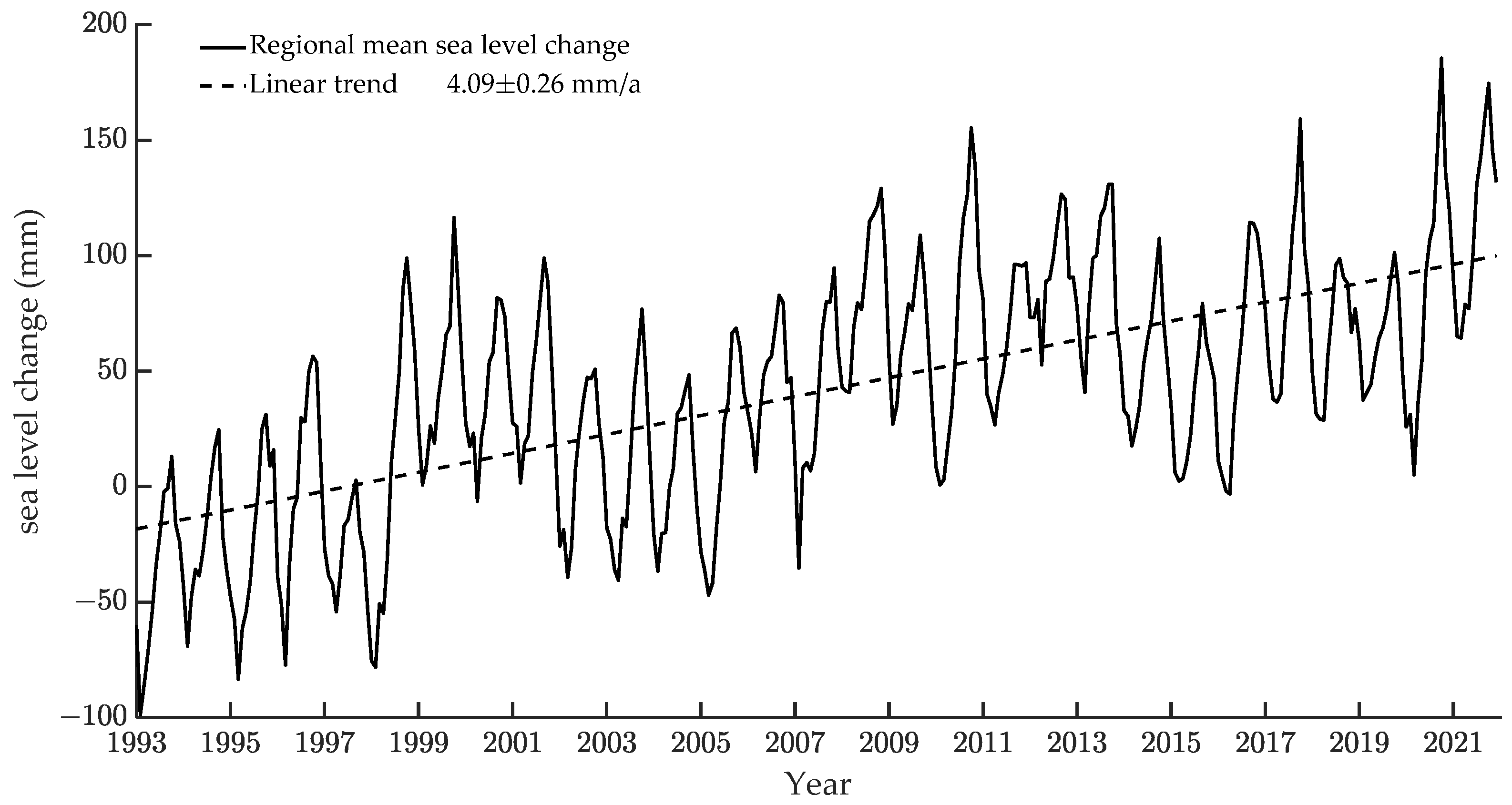
After regional averaging, a 29-year (348 months) sea-level-change time series for China adjacent seas was obtained, as shown in Figure 1. The least squares method is used to linearly fit the time series of sea level change in the adjacent seas of China from 1993 to 2021, and the annual change rate is 4.09 ± 0.26 mm/a (Figure 1). In order to better describe the sea-level-change datasets after the regional average, some statistical data of the datasets were obtained, such as the maximum (Max), minimum (Min), average, standard deviation (SD), and skewness. Table 1 shows the statistical results.

Figure 1.
Regional mean-sea-level-change series in the China adjacent seas and its linear trend for the period from 1993 to 2021.

Table 1.
The descriptive statistics of the sea-level-change datasets.
2.2. Singular Spectrum Analysis Method
SSA is based on the singular value decomposition (SVD) of a specific matrix constructed from the time series, which can extract signals of different components from a time series. This paper considers applying the SSA algorithm to the field of sea-level-change prediction to achieve the stabilization of the average sea-level-change time series. Let x = (x1, x2, …, xN) be a time series of length N (N > 1), where x is a non-zero sequence. Let an integer L (1 < L < N) represent the window length, and K = N − L + 1. The specific procedures of the SSA algorithm can be divided into the following four steps:
- Step 1: Embedding.
The original time series is mapped into a sequence of vectors with a length of L, forming K = N − L + 1 vectors with a length of L. These vectors constitute the trajectory matrix X.
- Step 2: Decomposition.
The trajectory matrix X is subjected to singular value decomposition (SVD), and the results are arranged in descending order. Let , be the eigenvalues of S, and . In this case, the trajectory matrix X can be decomposed as follows:
where is the number of non-zero singular values of X. is elementary matrices obtained from the singular value decomposition. represents the right singular vectors of X. represents the singular values of the covariance matrix. represents the left singular vectors of X.
- Step 3: Grouping.
Partition the index set {1, …, d} into p mutually disjoint subsets .
where is the subset matrix of linearly independent trajectory matrices obtained after grouping elementary matrices.
- Step 4: Diagonal mean.
By utilizing diagonal averaging, each matrix in Equation (4) is reorganized to obtain a new time series of length N. Let V be an L×K matrix with elements ,where and. Define and . If L < K, then ; otherwise,. By employing the following Equation (7) for diagonal averaging, the matrix V can be transformed into the time series as .
2.3. LSTM Neural Network
The LSTM neural network, initially proposed by Hochreiter and Schmidhuber [22], is a special type of recurrent neural network capable of effectively addressing the issue of long-term dependencies in information, avoiding the problems of vanishing or exploding gradients. It is suitable for handling and predicting significant events with long intervals and delays in time series data. LSTM comprises memory cells that can retain information over longer time intervals. These cells feature three gates: the input gate, output gate, and forget gate. These gates control the flow of information into and out of the memory cells, enabling LSTM to selectively remember or forget information. The specific principles of LSTM neural networks are presented as follows.
In the forget gate, unnecessary information can be chosen to be eliminated. It utilizes the output of the previous layer and the newly added input of the current layer as inputs, employing a sigmoid activation function, and as the output. The formula is as follows:
The input gate consists of two parts: one part is a sigmoid activation function, which outputs , and the other part is a tanh activation function, which outputs . The formula is as follows:
Through the calculations of the above two steps, we can compute the update value of the cell state at time t, denoted as . represents the amount of new information to retain. The formula is as follows:
The output gate is utilized to adjust the final output quantity of the cell state for that layer. Obtain using the sigmoid activation function; then, multiply by , processed through the tanh activation function, to obtain the output of this layer.
where , , and represent the weight matrix. , , , and represent the bias matrix.
2.4. SSA-LSTM
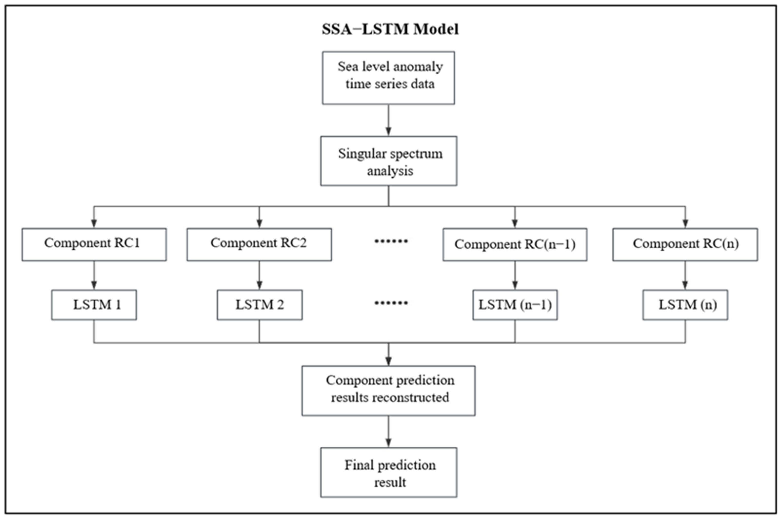
Based on the non-stationary and nonlinear characteristics exhibited by the sea-level-change time series, a SSA-LSTM hybrid prediction model was constructed in this study to analyze and predict the sea level change in the China adjacent seas. This approach significantly enhances the prediction accuracy for the non-stationary time series. The specific procedures are illustrated in Figure 2.
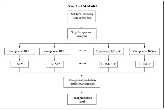
Figure 2.
The flowchart of SSA-LSTM hybrid prediction model.
Initially, the sea-level-change time series is decomposed by SSA to isolate the total time series as several components, such as the long-term trend, periods, and noise. This decomposition effectively transforms the non-stationary sea-level-change series into several relatively stationary sub-series, thereby reducing the complexity of the sea-level-change time series across multiple time scales. Subsequently, during the prediction process of the LSTM neural network model, a sliding window time series prediction method [23] is applied to establish an LSTM neural network prediction model. This model predicts each component using LSTM neural networks separately. Finally, all predicted results are added to obtain the final prediction result.
2.5. Evaluation Indices
To evaluate the prediction accuracy of the developed models, three evaluation indices, including the root mean square error (RMSE), mean absolute error (MAE), and coefficient of determination R2, are adopted. R2 reflects the quality of model fitting. A higher R2 value closer to 1 indicates a better model fit. RMSE is estimated as the square root of the ratio of the sum of squared differences between predicted and true values to the number of observations. MAE is the average of the absolute differences between predicted and true values, providing a better reflection of the actual errors in the predictions. The equations for calculating R2, RMSE, and MAE are presented as follows:
where represents the predicted values. represents the true values.
3. Results
3.1. Utilization of SSA
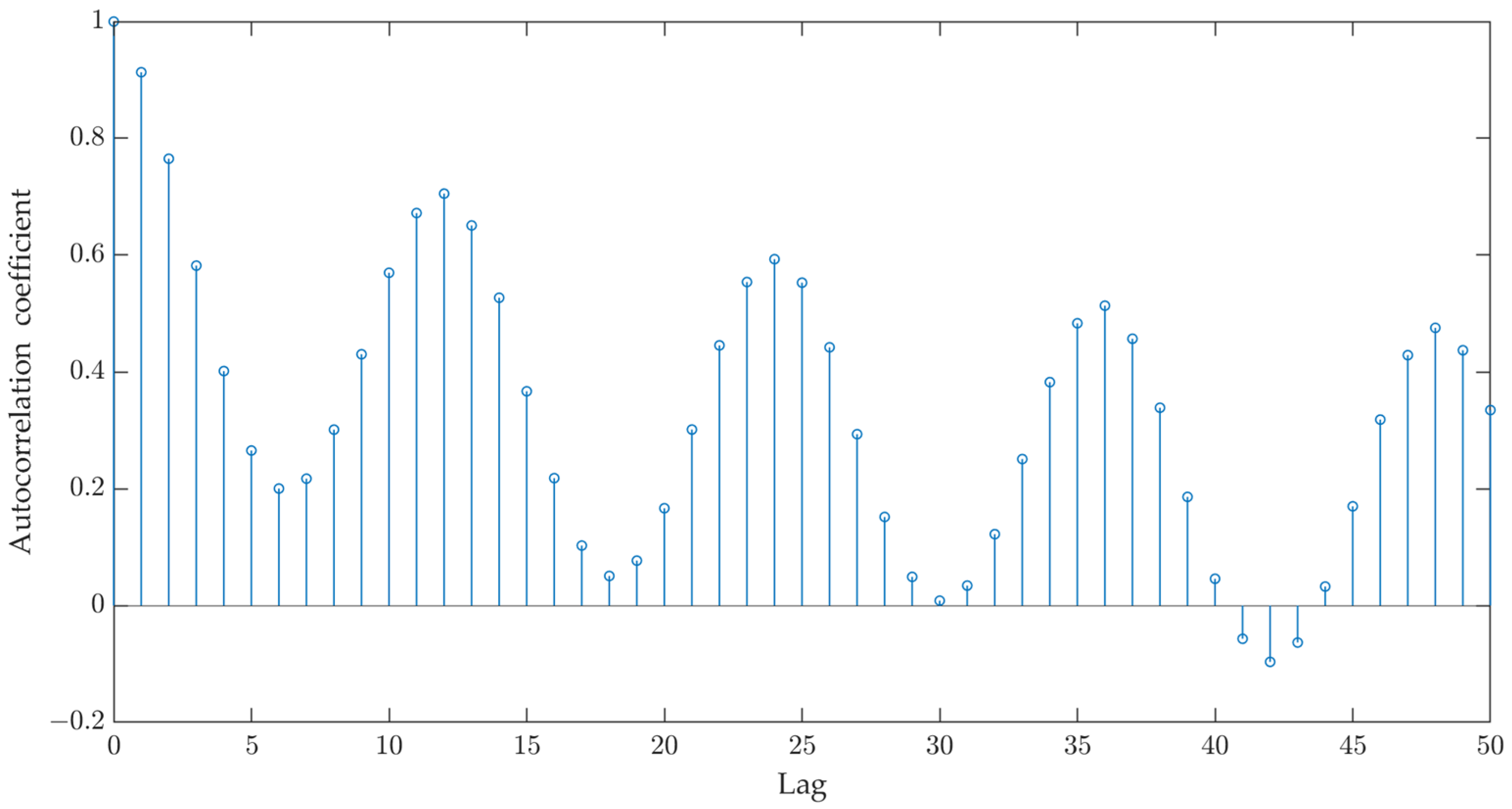
As mentioned earlier, sea level changes are influenced by multiple factors and exhibit characteristics, such as non-linearity, non-stationarity, and multi-scale variations. Decomposition–reconstruction methods can effectively reduce the complexity of the original sequence, thereby improving prediction accuracy. Prior to conducting SSA on the sea-level-change series, it is necessary to determine the window length. In this study, we utilized autocorrelation analysis to analyze the original time series [24], as shown in Figure 3. It is evident from the analysis that the sea-level-change series exhibits a significant periodic variation with a 12-month cycle. Therefore, the window length was set to 12 based on this observation.
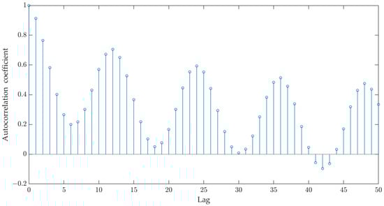
Figure 3.
Result of autocorrelation analysis of the original sea-level-change series.
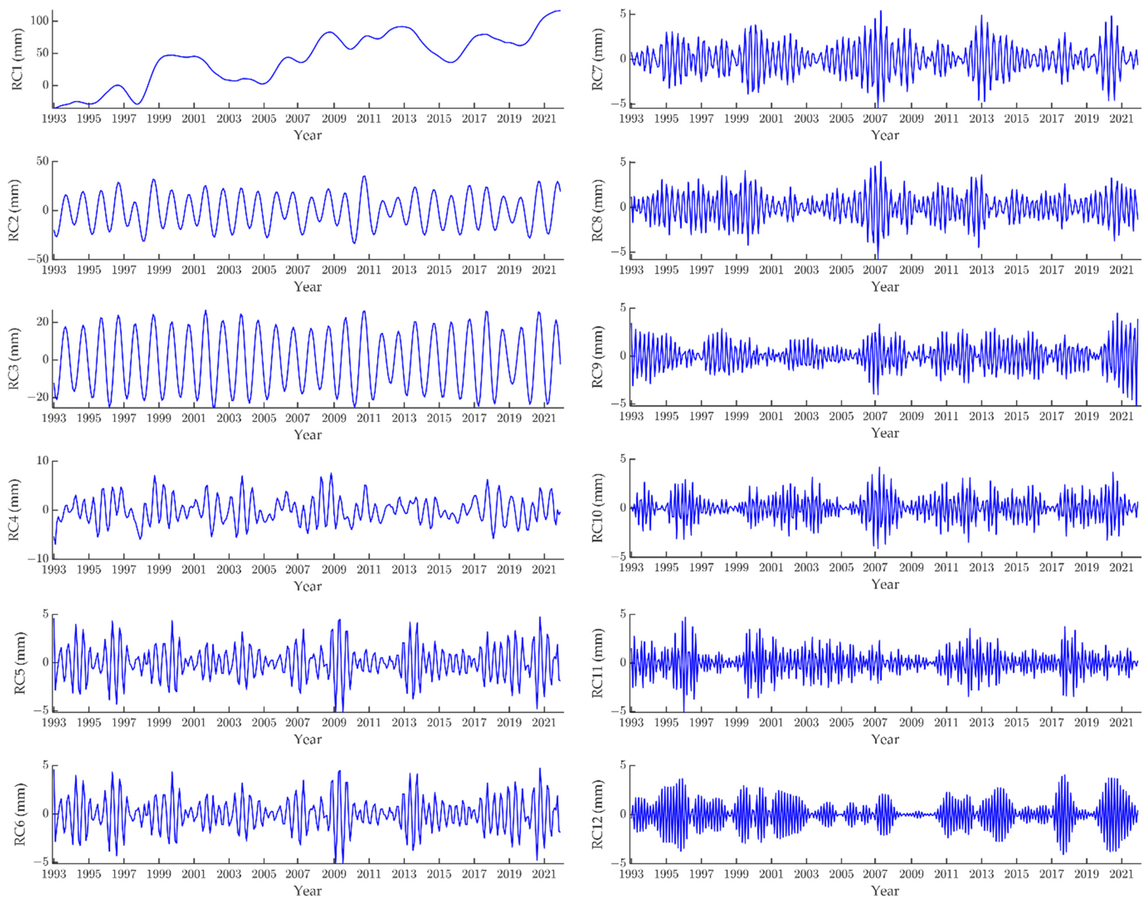
Based on the autocorrelation analysis results, a window length of 12 was determined to construct the trajectory matrix. As illustrated in Figure 4, the frequency domain of the SSA-transformed time modal sub-series appears stable. By conducting a least-squares linear fitting analysis on the long-term trend of the first reconstructed component RC1, the estimated regional mean sea-level-change rate is 3.95 ± 0.13 mm/a for the China adjacent seas, with a smaller 0.14 mm/a than 4.09 ± 0.26 mm/a (Figure 1) derived from the original sea-level-change series for the period from 1993 to 2021, due to the impact of other components, especially the periodic signal.
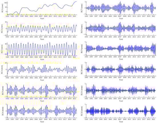
Figure 4.
The reconstructed components of sea-level-change series using the SSA approach.
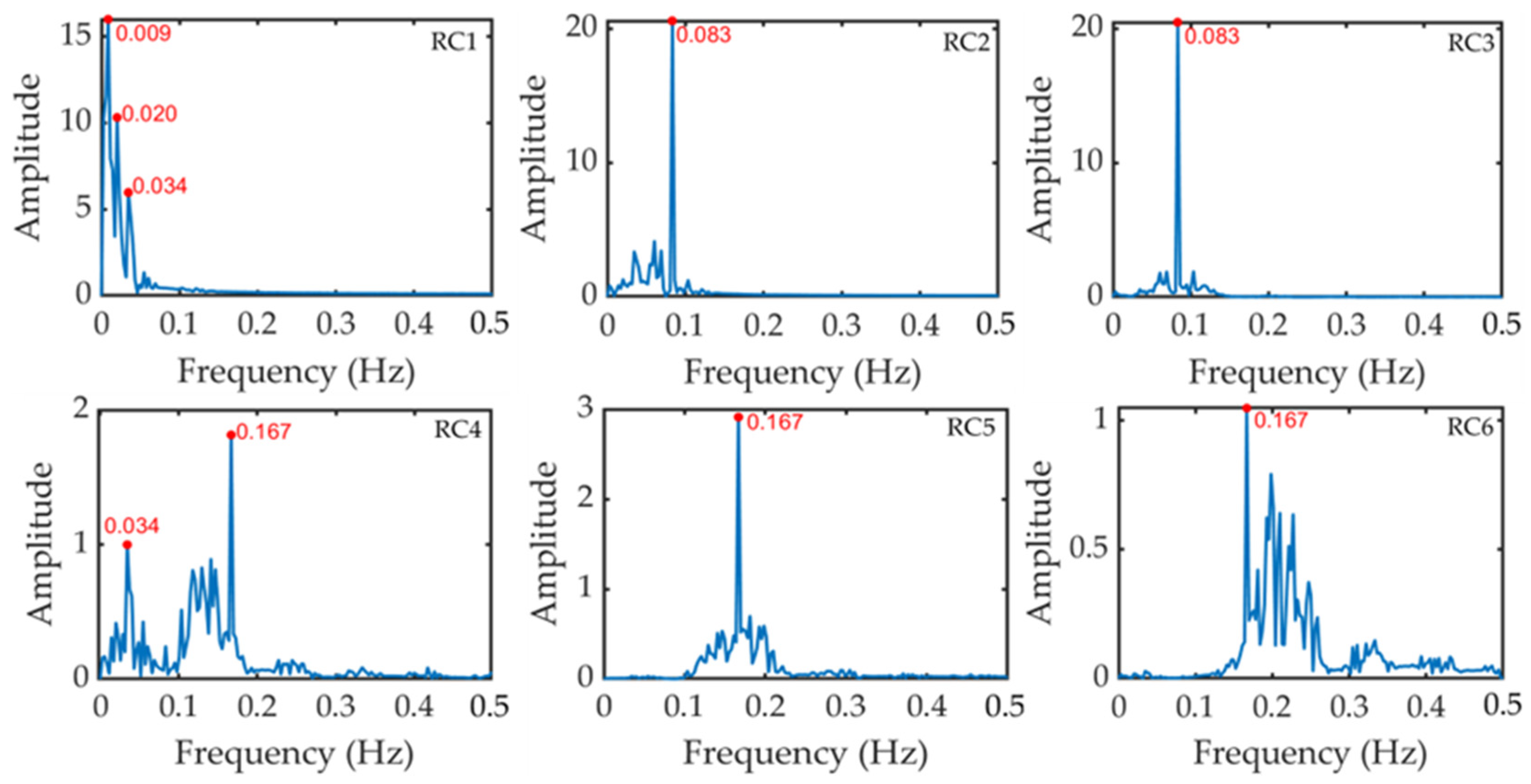
By performing frequency spectrum analysis on RC1 to RC12, sequentially, we identify the main periods associated with each component. When calculating the frequency axis, it is assumed that the unit time interval is 1. The RC1 to RC6 components have a significant main period, and RC7 to RC12 have no obvious main period, so the spectral period plots of the first six RC components are given, as shown in Figure 5. The red dots represent the main period, and the red numbers are the coordinates of the X axis. For RC1, the main period is 111 months (9.3 year), with additional periods of 50 months (4.2 year) and 29 months (2.4 year). These cyclical changes may reflect some physical phenomena [25,26]. The 9.3-year period likely reflects changes in lunar declination. The 4.2-year period variations may be associated with the El Niño-Southern Oscillation (ENSO) events occurring at intervals of 3 to 7 years. The 2.4-year period corresponds to oscillations with a 2-to-3-year cycle, primarily influenced by hydrological and meteorological factors along the China coast. RC2 and RC3 exhibit a main period of the annual cycle, indicative of pronounced annual variations. RC4, RC5, and RC6 all display a primary period of 6 months, associated with a semi-annual cycle, where RC4 exists for a 2.4-year cycle.
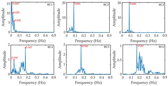
Figure 5.
The spectral periods of RC1–RC6.
3.2. Regional Mean Sea Level Change Prediction Using the SSA-LSTM Model
To predict the regional mean sea level changes, this study adopts a sliding window LSTM neural network prediction method. Specifically, the historical sea-level-change data from the preceding 12 months are utilized to predict the sea level change for the current month. The sea-level-change datasets spanning 348 months are divided into two parts: a training set and a test set. The first 278 months of data (from January 1993 to February 2016, approximately 80% of the data) are used for training, while the subsequent 70 months of data (from March 2016 to December 2021, approximately 20% of the data) are used for testing. To ensure effective model training and prevent divergence during training, the training and testing data are standardized before input. The grid search algorithm was used to optimize the hyperparameters. The grid search algorithm is a kind of exhaustive method, which determines the spatial dimension of the grid search according to the number of parameters, divides the grid in each dimension, and then traverses all the grid intersections to determine the best parameters according to the results given by the grid intersections. In this paper, the number of hidden layers is 1, and the step size is determined to be 12, so the value range of 3 hyperparameters is preset, the value range of the initial learning rate is [0.001, 0.01, 0.1], the value range of the number of iterations is ∈ [100, 250, 500, 1000], and the value range of the hidden layer neuron node is [8, 16, 32, 64, 128]. Finally, the objective function is set as the root mean square of the model test error as the minimum. After massive experimentation and tuning, an LSTM neural network model is established with the following hyperparameters: Adam optimization algorithm, a time step of 12 months for input sequences, a prediction step of 1 month, 16 nodes in the hidden layer, a maximum of 500 iterations, and an initial learning rate of 0.01. Other hyperparameters of the LSTM neural network model are set to default values. In the MATLAB 2019b compilation environment, the MATLAB toolbox was used to construct the LSTM neural network model.
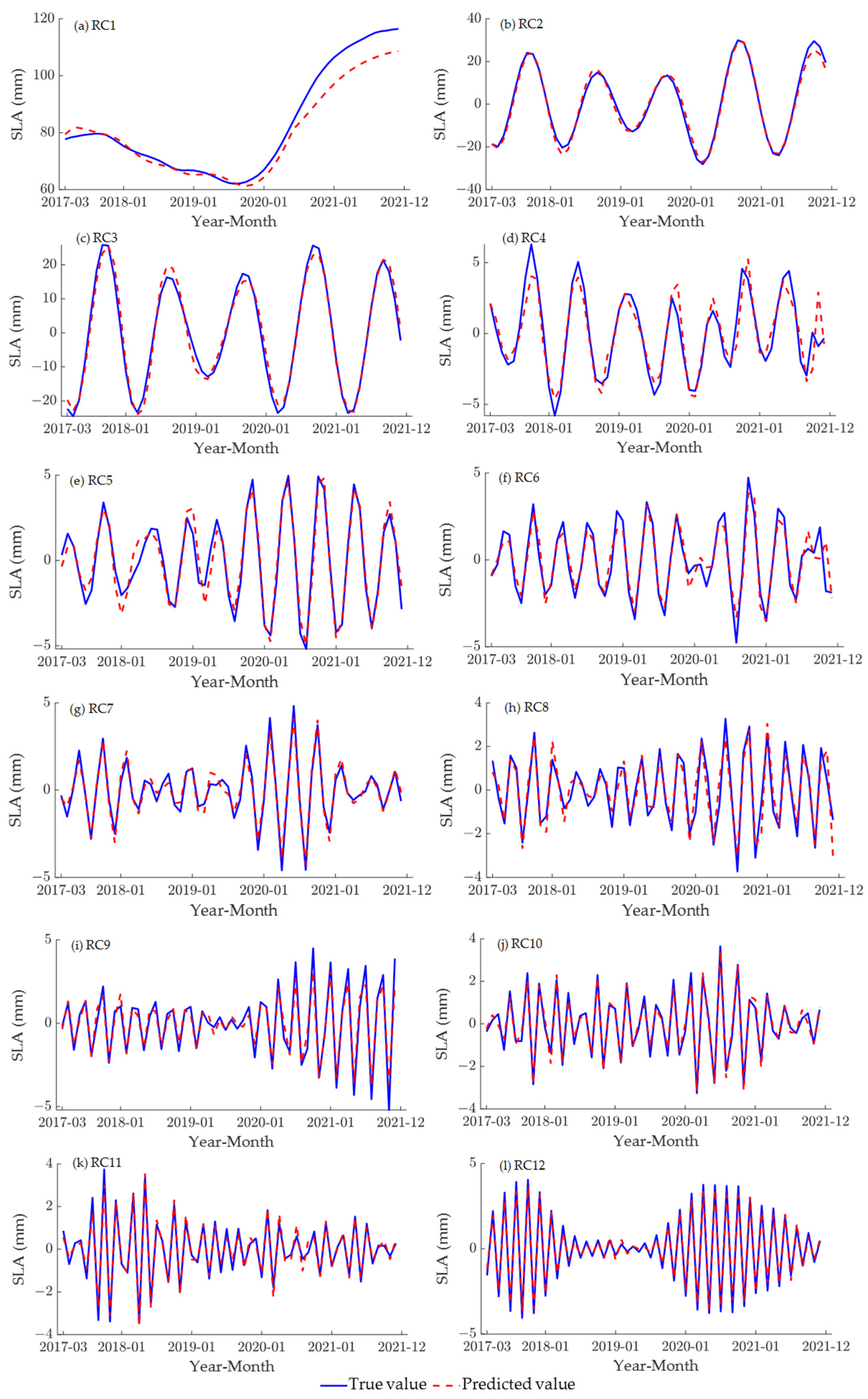
Decomposing the sea-level-change series using SSA to obtain RC1–RC12, a total of 12 principal component series, each component was individually predicted using the LSTM neural network model. The predicted results of these components were compared against the test datasets, as illustrated in Figure 6. From the observations in Figure 6, it is apparent that the predicted results of the components via SSA decomposition exhibit favorable performance. Particularly, segments of the component sub-series displaying strong periodicity demonstrate exceptionally good prediction accuracy.
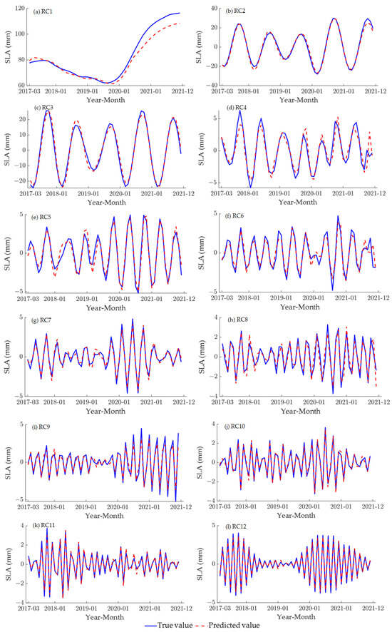
Figure 6.
Comparison of RC1–RC12 component prediction values with test set samples.
3.3. Evaluation of Prediction Results
To evaluate the prediction performance of the SSA-LSTM hybrid model, predictions are compared between the LSTM neural network model and the SSA-LSTM hybrid model. Additionally, the existing EMD-LSTM and CEEMDAN-LSTM hybrid models are included for a comparison to assess the prediction accuracy of the hybrid models. When applying the LSTM neural network model, EMD-LSTM hybrid model, and CEEMDAN-LSTM hybrid model, the dataset demarcation and hyper-parameter settings used in the SSA-LSTM hybrid model are maintained. The prediction results of the SSA-LSTM hybrid model and the other three models are shown in Figure 7. The prediction results of the other three methods demonstrate satisfactory performance, with overall amplitudes and trends closely matching the original data and exhibiting high prediction accuracy. The EMD-LSTM and CEEMDAN-LSTM hybrid model prediction performance is better at extreme points compared to the LSTM neural network model. This indicates that when applying LSTM neural networks for prediction, hybrid models achieve higher accuracy at extreme points compared to single prediction models. The SSA-LSTM model used in this study demonstrates a fitting effect that closely aligns with the original data. Additionally, its prediction performance at extreme points surpasses that of the other two hybrid models, showcasing superior prediction accuracy. This highlights the effectiveness of the SSA-LSTM hybrid model in improving prediction accuracy at extreme points within the context of long-term trend prediction research.
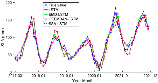
Figure 7.
Comparison of the predicted and true values of the four models.
To further analyze the fitting effectiveness and prediction accuracy of the four methods, this study evaluates all prediction results using precision metrics, such as R2, MAE, and RMSE, as shown in Table 2. From Table 2, it can be observed that the SSA-LSTM hybrid model achieves an R2 value of 0.98, significantly higher than that of the LSTM model and EMD-LSTM hybrid model, indicating a notable improvement in model fitting effectiveness. The prediction accuracy of the SSA-LSTM hybrid model surpasses that of the other three models, demonstrating highly desirable prediction results. Compared to the LSTM neural network model, the SSA-LSTM hybrid model exhibits a substantial increase in prediction accuracy. Additionally, compared to the other hybrid models, there is a notable enhancement in prediction accuracy with the SSA-LSTM hybrid model. The MAE of the SSA-LSTM hybrid model is higher compared to the other three hybrid models by 42.45%, 57.76%, and 63.99%, respectively. Similarly, the RMSE of the SSA-LSTM hybrid model is higher compared to the other three hybrid models by 41.69%, 60.83%, and 67.98%, respectively.
Table 2.
Comparison of error estimates of four prediction models.
4. Discussion
To enhance the prediction accuracy of sea level change, a combined model, namely SSA-LSTM model, is proposed in this study. The model employs the decomposition–prediction–reconstruction approach, which specifically includes the following: (1) decomposition: decompose the sea level change series into multiple components; (2) prediction: forecasting each component using the LSTM model; (3) reconstruction: reconstructed the final prediction by summing all predicted components. The results show that the proposed SSA-LSTM model can forecast the sea level change with a relative high accuracy. The core idea behind the proposed SSA-LSTM model is to combine the strengths of SSA in extracting information features of sea level change and the capabilities of the LSTM neural network in predicting sea level change. Given the nonlinear and non-stationary nature of the sea-level-change series, which exhibits distinct characteristics across different time scales, the SSA method is employed to preprocess the sea-level-change data, significantly reducing its non-stationarity. The LSTM model has the advantage for processing long-term dependencies in sequence data, making it particularly suitable for modeling problems with long-term sequential dependencies.
To investigate the impact of various data decomposition approaches to the LSTM model, two additional data decomposition methods, i.e., EMD and CEEMDAN, are also used as the comparison with respect to the SSA approach. Regarding the hyper-parameter setting in the deep learning model, we adopt the straightforward and efficient grid search algorithm. While this preprocessing method can determine the hyperparameters efficiently, we acknowledge the limitations of not exploring other techniques. Various methods of hyper-parameter optimization, such as Bayesian optimization and particle swarm optimization, may further enhance the model’s performance. Future research will involve an empirical evaluation of these techniques to assess their impacts on the model’s efficiency and accuracy, with the goal of identifying the most effective pre-processing strategies to improve the LSTM model.
In this study, the LSTM model uses single-step forecasting to predict the sea level change of one future month using the 1-year (12 months) historical data. As a result, the SSA-LSTM model has the advantage for short-term sea-level-change prediction. Currently, we have not conducted research on multi-step prediction or rolling prediction with the SSA-LSTM model. In future studies, we will consider extending the length of the dataset and employing multi-step forecasting methods to predict values for multiple months, aiming to achieve long-term forecasting of sea level change.
When considering the sea-level-rise trend, we applied the least squares linear fitting method to fit the original data and the long-term trend component of the first recon-structed component (RC1), and the estimated change rates are 4.09 ± 0.26 mm/a and 3.95 ± 0.13 mm/a, respectively. One standard deviation is used to estimate the velocity uncertainty. The estimated sea-level-change rate aligns with the recorded sea-level-rise trend in offshore China and is higher than the global sea-level-change rate during the same period. As the previous studies pointed out, global sea level rise is primarily driven by the thermal expansion of ocean water due to climate warming, along with the melting of land glaciers and polar ice caps [27,28,29]. However, significant regional differences existed in global sea level rise. The sea level change in China adjacent seas is also influenced by local regional hydrometeorological factors. Additionally, land subsidence can contribute to the relative rise in the local sea level. In future work, we plan to compare the experimental results with global and other regional data (outside of China) to explore the differences in the characteristics of sea level change between offshore China and other regions.
5. Conclusions
Using a latitude–longitude area-weighting method, this study computed regional averages of grid sea level anomaly data spanning the China adjacent seas from 1993 to 2021, thereby deriving a time series of sea level variations. Combining SSA with LSTM neural networks, an SSA-LSTM hybrid prediction model is established to predict the sea level change. The predicted results of the SSA-LSTM hybrid model are compared and analyzed against those of the LSTM neural network model, EMD-LSTM hybrid model, and CEEMDAN-LSTM hybrid model. The results demonstrate that utilizing SSA to process the regional mean sea-level-change series in the China adjacent seas from 1993 to 2021 reveals various periodic changes, including annual and semi-annual cycles, ENSO events, and variations related to lunar declination. The linear trend is 3.95 ± 0.13 mm/a derived from the RC1 component, which is closely consistent with the original sea-level-rise rate of 4.09 ± 0.26 mm/a, indicating that the SSA method effectively extracts the long-term trend and periodic variations in sea level change [30,31].
The prediction accuracy of the SSA-LSTM model is significantly higher than that of single LSTM neural network prediction model and several other hybrid prediction models. It can be observed that the prediction results are quite favorable. Especially, the SSA-LSTM hybrid model can significantly improve the prediction accuracy at extreme points, which exhibits a more reasonable fitting effect and notably enhances predictive accuracy, demonstrating good applicability in sea-level-change prediction.
Author Contributions
Conceptualization, Y.X. and S.Z.; Methodology, Y.X.; Validation, F.W.; Formal analysis, S.Z.; Resources, F.W.; Writing—original draft, Y.X.; Writing—review and editing, F.W.; Visualization, Y.X.; Supervision, S.Z.; Project administration, F.W. All authors have read and agreed to the published version of the manuscript.
Funding
This work is funded by the National Natural Science Foundation of China (42374017, 42064001).
Institutional Review Board Statement
Not applicable.
Informed Consent Statement
Not applicable.
Data Availability Statement
Data used in this study are available via AVISO (https://www.aviso.altimetry.fr/en/data/products/sea-surface-height-products/global.html) (accessed on 16 September 2023).
Conflicts of Interest
The authors declare no conflicts of interest.
References
- Frederikse, T.; Landerer, F.; Caron, L.; Adhikari, S.; Parkes, D.; Humphrey, V.; Dangendorf, S.; Hogarth, P.; Zanna, L.; Cheng, L.; et al. The causes of sea-level rise since 1900. Nature 2020, 584, 393–397. [Google Scholar] [CrossRef] [PubMed]
- 2022 China Sea Level Bulletin, Ministry of Natural Resources of the People’s Republic of China, Beijing, 2023, 1–43. Available online: https://gi.mnr.gov.cn/202304/P020230412574327887976.pdf (accessed on 30 September 2023).
- Fang, S.; Hai, Z.H.I.; Long, L.H.; Lin, P.F. Analysis and Comparison of the Sea Level Rising Trend in the Marginal Seas around China. Clim. Environ. Res. Chin. 2016, 21, 346–356. [Google Scholar]
- Collins, M.; Allen, M.R. Assessing the Relative Roles of Initial and Boundary Conditions in Interannual to Decadal Climate Predictability. J. Clim. 2002, 15, 3104–3109. [Google Scholar] [CrossRef]
- Luo, W.; Yuan, L.; Yu, Z.; Yi, L.; Xie, Z. Regional Sea level change in Northwest Pacific: Process, characteristic and prediction. J. Geogr. Sci. 2011, 21, 387–400. [Google Scholar] [CrossRef]
- Grinsted, A.; Moore, J.C.; Jevrejeva, S. Reconstructing sea level from paleo and projected temperatures 200 to 2100 AD. Clim. Dyn. 2009, 34, 461–472. [Google Scholar] [CrossRef]
- Huang, N.E.; Shen, Z.; Long, S.R.; Wu, M.C.; Shih, H.H.; Zheng, Q.; Yen, N.-C.; Tung, C.C.; Liu, H.H. The empirical mode decomposition and the Hilbert spectrum for nonlinear and non-stationary time series analysis. Proc. R. Soc. A Math. Phys. Eng. Sci. 1998, 454, 903–995. [Google Scholar] [CrossRef]
- Wu, Z.; Huang, N.E. Ensemble empirical mode decomposition: A noise-assisted data analysis method. Adv. Adapt. Data Anal. 2009, 1, 1–41. [Google Scholar] [CrossRef]
- Ding, T.; Wu, D.; Li, Y.; Shen, L.; Zhang, X. A hybrid CEEMDAN-VMD-TimesNet model for significant wave height prediction in the South Sea of China. Front. Mar. Sci. 2024, 11, 1375631. [Google Scholar] [CrossRef]
- Golyandina, N.; Nekrutkin, V.; Zhigljavsky, A.A. Analysis of Time Series Structure: SSA and Related Techniques; CRC Press: Boca Raton, FL, USA, 2001. [Google Scholar]
- Anwar, S.; Rahman, K.; Bhuiyan, A.E.; Saha, R. Assessment of Sea Level and Morphological Changes along the Eastern Coast of Bangladesh. J. Mar. Sci. Eng. 2022, 10, 527. [Google Scholar] [CrossRef]
- Fu, Y.; Zhou, X.; Sun, W.; Tang, Q. Hybrid model combining empirical mode decomposition, singular spectrum analysis, and least squares for satellite-derived sea-level anomaly prediction. Int. J. Remote Sens. 2019, 40, 7817–7829. [Google Scholar] [CrossRef]
- Zhao, J.; Cai, R.; Fan, Y. Prediction of Sea Level Nonlinear Trends around Shandong Peninsula from Satellite Altimetry. Sensors 2019, 19, 4770. [Google Scholar] [CrossRef]
- Raj, N.; Gharineiat, Z.; Ahmed, A.A.M.; Stepanyants, Y. Assessment and Prediction of Sea Level Trend in the South Pacific Region. Remote Sens. 2022, 14, 986. [Google Scholar] [CrossRef]
- Fenghua, W.; Jihong, X.; Zhifang, H.; Xu, G. Stock price prediction based on SSA and SVM. Procedia Comput. Sci. 2014, 31, 625–631. [Google Scholar] [CrossRef]
- He, L.; Li, G.; Li, K.; Cui, L.; Ren, H. Multi-scale prediction of regional sea level change based on EEMD and BP neural network. Quat. Sci. 2015, 35, 374–382. [Google Scholar]
- Peng, S.; Chen, R.; Yu, B.; Xiang, M.; Lin, X.; Liu, E. Daily natural gas load forecasting based on the combination of long short term memory, local mean decomposition, and wavelet threshold denoising algorithm. J. Nat. Gas Sci. Eng. 2021, 95, 104175. [Google Scholar] [CrossRef]
- Gross, S. Recurrent neural networks. Scholarpedia 2013, 8, 1888. [Google Scholar]
- Zhao, J.; Cai, R.; Sun, W. Regional sea level changes prediction integrated with singular spectrum analysis and long-short-term memory network. Adv. Space Res. 2021, 68, 4534–4543. [Google Scholar] [CrossRef]
- Tur, R.; Tas, E.; Haghighi, A.T.; Mehr, A.D. Sea level prediction using machine learning. Water 2021, 13, 3566. [Google Scholar] [CrossRef]
- Balogun, A.-L.; Adebisi, N. Sea level prediction using ARIMA, SVR and LSTM neural network: Assessing the impact of ensemble Ocean-Atmospheric processes on models accuracy. Geomatics Nat. Hazards Risk 2021, 12, 653–674. [Google Scholar] [CrossRef]
- Hochreiter, S.; Schmidhuber, J. Long Short-Term Memory. Neural Comput. 1997, 9, 1735–1780. [Google Scholar] [CrossRef]
- Selvin, S.; Vinayakumar, R.; Gopalakrishnan, E.A.; Menon, V.K.; Soman, K.P. Stock price prediction using LSTM, RNN and CNN-sliding window model. In Proceedings of the 2017 International Conference on Advances in Computing, Communications and Informatics (ICACCI), Udupi, India, 13–16 September 2017; pp. 1643–1647. [Google Scholar]
- Chakravarti, I.M.; Box, G.E.P.; Jenkins, G.M. Time Series Analysis Forecasting and Control. J. Am. Stat. Assoc. 1973, 68, 712. [Google Scholar] [CrossRef]
- Yuan, L.; Yu, Z.; Xie, Z.; Song, Z.; Lü, G. ENSO signals and their spatial-temporal variation characteristics recorded by the sea-level changes in the northwest Pacific margin during 1965–2005. Sci. China Ser. D Earth Sci. 2009, 52, 869–882. [Google Scholar] [CrossRef]
- Wang, H.; Liu, K.; Fan, W.; Zhang, Q.; Zhang, Z.; Wang, G. The Relationship between Sea Level Change of China’s Coast and ENSO. In Proceedings of the Twenty-Fifth International Ocean and Polar Engineering Conference, Kona, HI, USA, 21–26 June 2015. [Google Scholar]
- Wang, F.; Shen, Y.; Chen, Q.; Sun, Y. Reduced Misclosure of Global Sea-Level Budget Using New Released Tongji-Grace 2018 Solution. Sci. Rep. 2021, 11, 17667. [Google Scholar] [CrossRef]
- Chen, Q.; Wang, F.; Shen, Y.; Zhang, X.; Nie, Y.; Chen, J. Monthly gravity field solutions from early LEO satellites’ observations contribute to global ocean mass change estimates over 1993~2004. Geophys. Res. Lett. 2022, 49, e2022GL099917. [Google Scholar] [CrossRef]
- Cazenave, A.; Dominh, K.; Guinehut, S.; Berthier, E.; Llovel, W.; Ramillien, G.; Ablain, M.; Larnicol, G. Sea Level budget over 2003–2008: A reevaluation from GRACE space gravimetry, satellite altimetry and Argo. Glob. Planetary Change 2009, 65, 83–88. [Google Scholar] [CrossRef]
- Meli, M.; Camargo, C.M.L.; Olivieri, M.; Slangen, A.B.A.; Romangoli, C. Sea level trend variability in the Mediterranean during the 1993–2019 period. Front. Mar. Sci. 2023, 10, 1150488. [Google Scholar] [CrossRef]
- Pandžić, K.; Likso, T.; Biondić, R.; Biondić, B. A review of the contribution of satellite altimetry and tide gauge data to evaluate sea level trends in the Adriatic Sea within a Mediterranean and Global Context. GeoHazards 2024, 5, 112–141. [Google Scholar] [CrossRef]

Disclaimer/Publisher’s Note: The statements, opinions and data contained in all publications are solely those of the individual author(s) and contributor(s) and not of MDPI and/or the editor(s). MDPI and/or the editor(s) disclaim responsibility for any injury to people or property resulting from any ideas, methods, instructions or products referred to in the content. |
© 2024 by the authors. Licensee MDPI, Basel, Switzerland. This article is an open access article distributed under the terms and conditions of the Creative Commons Attribution (CC BY) license (https://creativecommons.org/licenses/by/4.0/).