Identification of Key Habitats of Bowhead and Blue Whales in the OSPAR Area of the North-East Atlantic—A Modelling Approach towards Effective Conservation

Abstract

Effective protection of highly mobile and data-poor species constitutes a great challenge amid growing ocean exploitation and use. Blue whales and bowhead whales in the North-East Atlantic face several threats, such as climate change, ship strikes, pollution, and entanglement in fishing gear. Consequently, the OSPAR (“Oslo-Paris Convention for the Protection of the Marine Environment of the North-East Atlantic”) Commission recognised their need for protection and included them on the OSPAR List of Threatened and/or Declining Species. Two actions to protect these endangered species that OSPAR Contracting Parties have agreed on are (i) identifying areas that play an essential role in the species’ life cycle—subsequently called key habitats, and (ii) ensuring that those key habitats are covered by OSPAR marine protected areas (MPAs). In addition, OSPAR has committed to expanding its network of MPAs and other effective area-based conservation measures by 2030 to cover at least 30% of the OSPAR maritime area (termed the 30 × 30 target) from today’s approx. 11%. In this paper, we present the results of modelling key habitats for the bowhead and blue whales in the North-East Atlantic, including Arctic waters. Due to the sparse data situation for these species, we apply presence-only modelling methods. As this method can, in principle, produce somewhat biased results, we recommend that systematic, regular surveys on these species in Arctic waters be significantly intensified for future analyses to overcome the data paucity and allow using presence–absence/count data modelling approaches. Key habitats of blue whales were identified between Iceland and Svalbard, extending to the Azores. For bowhead whales, key habitats were identified in the Fram Strait. However, our findings show that only 11.8% of blue whale key habitats and 4.1% of bowhead whale key habitats are currently covered by OSPAR MPAs. To protect 30% of key habitats for these species in the most efficient way, our analyses suggest that suitable areas to designate new OSPAR MPAs are located around the Azores for blue whales and in the Fram Strait for bowhead whales. With these additional MPAs, OSPAR would substantially improve the protection of the two endangered species and, at the same time, progress towards its 30 × 30 target.

1. Introduction

Great whales are in a worrying state worldwide and urgently require enhanced protection. Given the increasing threats from human activities and ongoing climate change, the OSPAR (“Oslo-Paris Convention for the Protection of the Marine Environment of the North-East Atlantic”) Commission has recognised the necessity of implementing measures to safeguard these endangered species [1]. A critical aspect of protecting great whales is the identification and preservation of key habitats essential for their reproduction, feeding, and migration [2]. Marine protected areas play a pivotal role in this context by safeguarding these vital habitats from harmful influences [3]. However, there is still a significant lack of comprehensive data on the specific needs and distribution areas of many great whale species, impeding the planning and implementation of effective conservation strategies [4].

The OSPAR Convention is an international agreement on the protection of the marine environment of the North-East Atlantic. Fifteen countries and the European Union are Contracting Parties to the convention and work together to address pollution, biodiversity loss, habitat degradation, and sustainable resource use. By fostering cooperation, OSPAR aims to ensure the long-term health of the North-East Atlantic’s marine ecosystem. Important tools to achieve that are the OSPAR network of marine protected areas (MPAs) [5] as well as the OSPAR List of Threatened and/or Declining Species and Habitats [6] and an associated roadmap [7] that outlines actions to be implemented collectively or individually by Contracting Parties, to protect the listed species.

According to these actions, it should be examined if the key habitats of bowhead whale (Balaena mysticetus) and blue whale (Balaenoptera musculus) are covered by the OSPAR network of MPAs and if additional areas could be proposed as MPAs. Since OSPAR has subscribed to the 30 × 30 target, i.e., to protect 30% of its maritime area, which extends from the Strait of Gibraltar up to the North Pole by 2030, by designating new MPAs, OSPAR could make progress concerning two of its objectives, namely, to increase its MPA coverage from currently approx. 11% and to enhance the protection of these two endangered whale species.

In this study, we apply a modelling approach to identify the key habitats of bowhead and blue whales in the OSPAR maritime area, determine their coverage by existing OSPAR MPAs, and propose locations for new MPAs to increase that coverage. Thus, our results can contribute positively to improving the protection of bowhead and blue whales as well as the marine environment of the North-East Atlantic, including Arctic waters, in general.

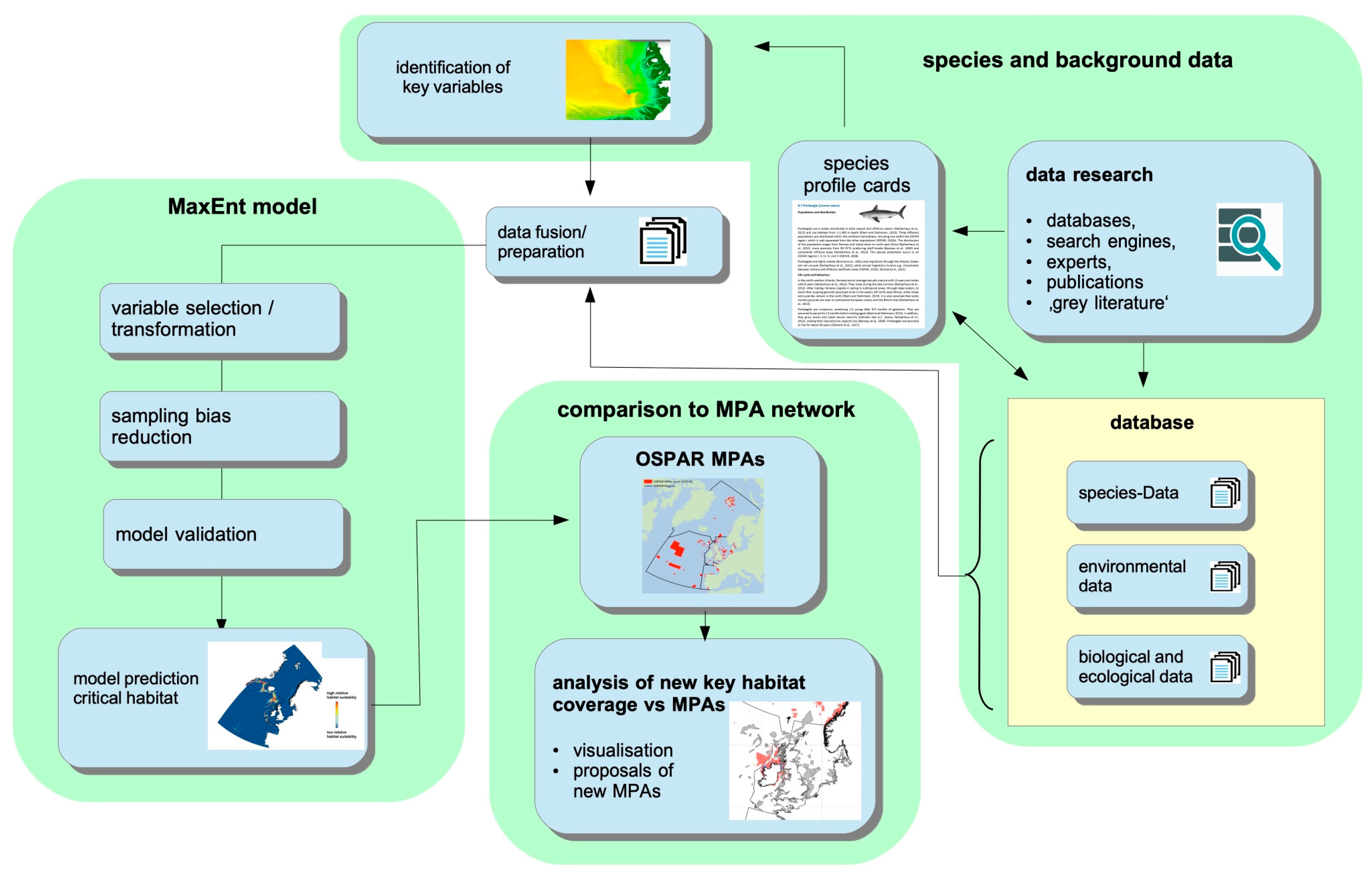
2. Materials and Methods

The OSPAR area is a very large area, covering approximately 13.5 million square kilometres and including parts of the Northeast Atlantic, the North Sea, the northwest continental shelf, and sections of the Arctic Ocean. Species data are therefore not available across the board and, in addition, vary greatly in nature, ranging from chance observations and tracking data to systematic survey data. Therefore, modelling key habitats requires the development and application of statistical methods capable of dealing with such data heterogeneity [8] and the acquisition of appropriate covariates given in the entire region.

In order to maximise the data basis for modelling on the one hand and to optimise the interaction between data and the various decisions in the context of variable selection and modelling technology on the other, the following approach was chosen and presented in this work:

First, intense worldwide research and acquisition of datasets on the distribution of the above species in the OSPAR area were conducted based on species databases, search engines, marine mammal experts, publications, and “grey literature”. In addition, scientific information on the ecology and biology of the above species was gathered and the results were validated by several species- and/or region-specific experts (summarised in the Supporting Material S3). Furthermore, suitable biotic and abiotic variables for modelling were selected based on biological and ecological characteristics (e.g., life cycle) of the species.

The second aim was the development of a robust modelling approach for the spatial identification of key habitats of the above-mentioned species. A particular focus was given to the development of appropriate statistical methods that can integrate data from different sources. Indeed, ecological data usually contain a number of statistical challenges, e.g., (but not exclusively) overdispersion, spatial and temporal autocorrelation, sampling bias and/or nonlinear correlations [9,10,11,12,13], making the choice and development of appropriate techniques non-trivial.

Third, we applied these methods to the above-mentioned data and subsequently aligned the modelled key habitats with the OSPAR network of MPAs. This included the identification of gaps in the OSPAR network of MPAs based on the identified key habitats and thus provides a scientifically sound and empirically well-founded proposal for additional MPAs to improve the protection of blue whales and bowhead whales in the OSPAR area.

A schematic overview of the overall approach is shown in Figure 1 and can be divided into three different work packages, namely (1) the research and acquisition of species and background information and data, (2) the development and application of appropriate modelling techniques, and (3) the comparison of the predicted key habitats with the existing OSPAR MPA network.

2.1. Species Data: Sources, Preparation and Suitability for Modelling

In order to obtain sufficiently high spatial coverage of the entire OSPAR maritime area, species data have been acquired from various sources. “High-quality data” (e.g., highly standardised survey data specialised/optimised for the species of interest such as, e.g., data from the SCANS surveys [14]), as well as data from less standardised approaches (e.g., data from presence-only databases), were gathered. The latter datasets were also considered, as no estimation of absolute animal numbers/densities was required, and thus, no method-specific correction factors for availability and/or visibility bias had to be derived. Instead, only relative changes in habitat suitability in space were of interest. Modelling of relative habitat suitability was carried out using the data as presented in Supporting Material S1 in detail.

In summary, the available survey data (i.e., data comprising both positive and zero observations) with respect to the blue whale resulted in 988,339 entries comprising only 14 sightings of individuals or groups, and for presence-only data, we obtained 427 positive sightings of one or more individuals. With respect to the bowhead, 22 positive sightings were available in the survey data, but 286 were in the presence-only data. Spatial plots of all data (separately for survey vs. presence-only data) are given in Figure 2. Because survey data comprised too few positive observations for regression-based modelling (e.g., using appropriate regression techniques [8]), the analysis used was based on the MaxEnt approach particularly suited for presence-only data (more corresponding details are given below). Particularly if data are sparse, MaxEnt was shown to still show reliable predictions [15]. In addition, if count data are sparse (i.e., many zeros and few ones), the random distribution of a count-data model would approximate a Bernoulli distribution so that cropping values > 1 (which happens in the course of presence-only methods) has an increasingly negligible influence on the predicted patterns with sparse data.

Of course, presence-only data were augmented with positive observations based on survey data.

All species data have been restricted to the period 2000–2022, aiming to find the optimal compromise between a long enough time series to produce sufficient data, even for rare species, while not using data that might reflect historical rather than actual distribution patterns and habitat preferences. However, for several datasets, the survey/observation effort was not equally distributed with respect to the time of year. In particular, survey data in the Arctic region were biased towards the summer. Consequently, the final predicted key habitats are also assumed to be biased towards the main survey season.

2.2. Definition of “Key Habitat” in the Context of the Project

Due to sparse data (in particular with respect to age and sex classes), key habitats were modelled based on maximum data, comprising observations from all sexes and age classes. The modelling approach modelled key habitats in terms of habitat suitability. Here, only the relative values of habitat suitability are relevant because areas of particular relative importance are to be extracted rather than total values of abundance or density. Predicted species-specific values were thus rescaled to values ≤ 1 to facilitate inter-species comparability. The resulting patterns of relative habitat suitability do not necessarily correspond to the (relative) animal distribution or abundance [16], but both are assumed to be strongly related without existing barriers to animal movement. Hence, during validation/plausibility checking of model results (e.g., in the context of previous works investigating abundances), no strict distinction between (relative) species abundance and (relative) habitat suitability was applied. However, the aim was to indeed model habitat suitability instead of abundance in a reasonable range around the observation (cf., “buffer” below) since abundance could be already influenced by anthropogenic activities and suitable habitats are to be identified, which can be used by the species if disturbance is minimised. For the considered species, this difference is, however, rather academic in practice because, in almost all cases, the identified key habitats coincide with high abundance (cf., Results and Discussion Sections).

2.3. Predictor Variables: Sources and Preparation

Potential predictor variables have been acquired from various sources and with varying spatial and temporal coverage and resolution. Like the species data, the aim was not to use variables with optimal spatio-temporal resolution only but rather to acquire data for all variables that may have a significant effect on species distribution as suggested by our species-specific background analyses (cf. Supporting Materials S3 and S4). Spatial data gaps (frequently occurring, e.g., very close to the coastline) have been extrapolated by assigning the value of the spatially closest pixel with existing information to each missing-value pixel (“nearest-neighbour approach”).

All variables have also been used/tested as log-transformed values, which can improve model performance by normalising skewed data, reducing heteroscedasticity, and capturing nonlinear relationships. Furthermore, it is often assumed that the spatial derivative, rather than the variable itself, is the important predictor, i.e., ocean regions with strong environmental gradients, such as oceanic fronts (e.g., represented by gradients in salinity and/or temperature) or continental slopes (i.e., gradients in water depth), are often of particular ecological importance [17,18]. To describe such dependencies, the spatial gradient for each variable has also been calculated and tested. Finally, for each variable, the spatial gradient of the log-transformed measure has been calculated and tested. Details with respect to the different variable sources are given in the Supporting Material S4.

2.4. Statistical Methods

Modelling approach. The following statistical methods were developed and applied to predict relative habitat suitability representing species-specific key habitats. Initially, we tested and applied two distinctly different modelling approaches to the data to provide appropriate methods for different data situations, namely regression-based methods for count-data (related to those of Mercker et al. [8]) and methods for presence-only data. In particular (and as mentioned above), data were usually given either in terms of systematic survey/count data or as occurrence/presence-only data.

Although analyses based on survey data (thus quantifying and correcting for effort) generally lead to more reliable results if the data density with respect to positive observations is comparable, presence-only methods will perform better if the density of presence-only data greatly exceeds that of positive observations in survey data, and/or if regions frequently used by the species under consideration are reflected in presence-only data but are completely absent in survey data. In each of these scenarios, the advantages of the higher data density of positive observations (and/or the better spatial coverage) outweigh the disadvantages of presence-only methods vs. count-data methods.

Thus, for both considered species, the species distribution modelling (SDM) algorithm MaxEnt [15,16] was used, which is based on the maximum entropy principle and is strongly related to an inhomogeneous Poisson point process [19,20]. In particular, presence observations were augmented with 10,000 pseudo-absences, randomly selected in a spatial buffer (cf., below) around the presence observations. The statistical advantages of MaxEnt (e.g., efficient handling of complex response-predictor interactions, ability to deal with small sample sizes), in conjunction with its simplicity of use, have led to the fact that it is currently the most widely used SDM algorithm [21].

However, such presence-only methods are sensitive, dependent on the survey design, and thus might not always reflect animal presence (respectively habitat suitability) as the results may be confounded by survey effort [22] if sampling bias is present [21]. If, for example, data are only obtained in a specific region (e.g., whale observations from ships associated with the coast), MaxEnt might interpret high sampling efforts as hotspots of species presence. An efficient bias-correction method, “Systematic Sampling” [21], was thus applied before using MaxEnt. In addition, sampling bias was further reduced by including expert/literature knowledge, particularly by pre-selecting the predictors based on known preferences for each considered species [23] and by applying efficient variable selection techniques [24]. In summary, several steps were used to prevent or minimise the effect of sampling bias, including thinning presence data (keeping only one occurrence point per spatial grid cell), creating dummy points only within a spatial buffer around presence points (with a buffer width adapted to the mobility/spatial spread of the considered species), applying efficient variable selection techniques (cf., below) and integrating expert knowledge at several points of the analysis.

Variable/model selection and validation. Considering the variety of predictor variables (including their various transformed variants—cf., above and Supporting Material S4), it is of particular importance to apply efficient variable selection techniques before final modelling. This leads to the selection of the most predictive subset of theoretically reasonable variables and, thus, to the ecologically most reasonable (and parsimonious) models [24]. In this study, variable selection was based on the methods described by Vollering et al. [24]. Several additional transformations were applied (e.g., representing both nonlinear dependencies as well as threshold-like behaviour), and appropriate variables were finally selected based on subset selection methods, which appear to outperform other selection methods (e.g., LASSO) in the context of MaxEnt [24]. Model validation was also based on the methods described by Vollering et al. [24].

Software. All statistical analyses were carried out using the open-source software R [25]. MaxEnt analysis was carried out using the R-package MiaMaxent [24], and visualisation and spatial analyses using the R-packages ggplot2 [26], raster [27,28], sf [29], and spatstat [30]. In addition, further data manipulation utilised the R-packages lubridate [31], RANN [32] and plyr [33].

Prediction of relative habitat suitability. Predictions of relative habitat suitability were based on the different predictor variables given for the entire OSPAR area using predict functions provided by the corresponding R-packages. However, a few adaptions were made.

First, predictions were not made for the entire OSPAR area (which might include unrealistic/highly speculative extrapolations) but rather for spatial buffers around reported occurrence points. Here, the size of the buffer has been adapted to the spatial spread of presence points in the raw data and was set to a radius of 200 km for the blue whale and to a radius of 500 km for the bowhead whale since blue whale observations appear to be more locally clustered compared to the bowhead observations (Figure 2). Subsequently, only those buffers comprising more than two occurrence points have been considered (to exclude single false-positive observations). In addition, the robustness of model predictions was tested with respect to changes in buffer size.

Second, minimum and maximum values of predictor variables in the entire OSPAR area were cropped to the minimum and maximum values of these variables associated with the species observation data points (i.e., to the experimentally assessed range), which reduces problems connected with extrapolation. Finally, we rescaled the final predicted relative habitat suitability patterns for optimal comparability, such that the maximum values were equal to 1.

Estimation of prediction uncertainties. To estimate prediction uncertainties, the methodological approach was based on 10 different resamples (i.e., “random draw with put back” of lines) of the original data frame used for modelling, where the difference between minimum and maximum values from the predictions for each spatial pixel was presented (Supporting Material S2). This roughly corresponds to the (spatially varying) extent of the 90% confidence intervals for the relative habitat suitability. Notably, uncertainties connected with the intercept have been neglected (in contrast to approaches where the total abundance or density is estimated) because only the relative changes in space were important.

Derivation of locations suitable for new/additional MPAs. To identify areas suitable for new/additional MPAs, the following additional aspects were taken into account:

• Different species show different degrees of “patchiness” with respect to the distribution of (and strength of association with) key habitats. Thus, different sizes of protected areas are required to achieve the same strength/percentage of protection;
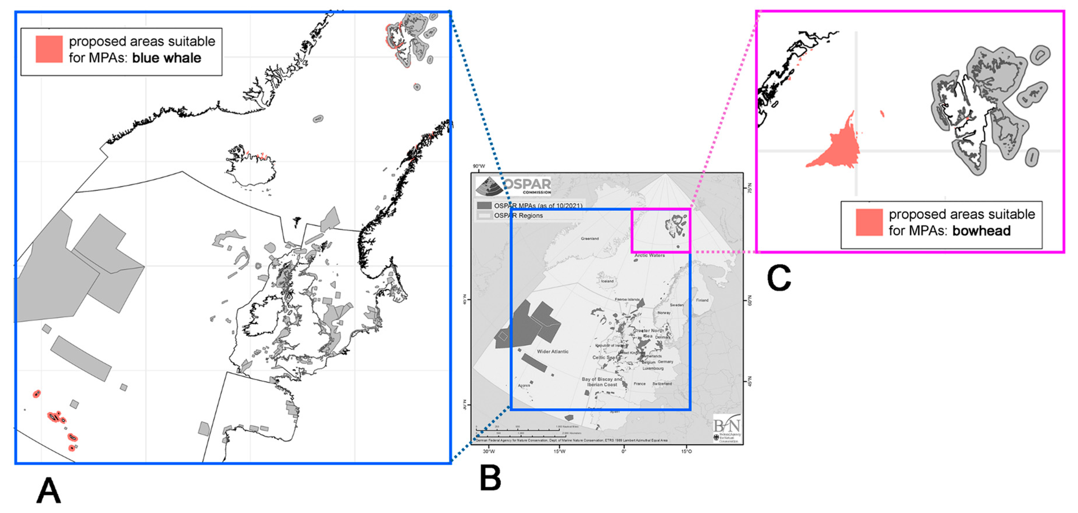
• the percentage of key habitats already protected by MPAs, and thus, the need for additional MPAs varies among species;
• our predicted key habitats differ in their quality of prediction, depending on both species and location (Supporting Material S2);
• for some of the species/identified locations for MPAs, protection measures may suffice for certain periods of the year (migratory species, breeding season);
• predicted key habitats of species can overlap, which increases the overall contribution of potential MPAs at those locations;
• MPAs should not be too fragmented and/or small (e.g., comprising only a few km²).

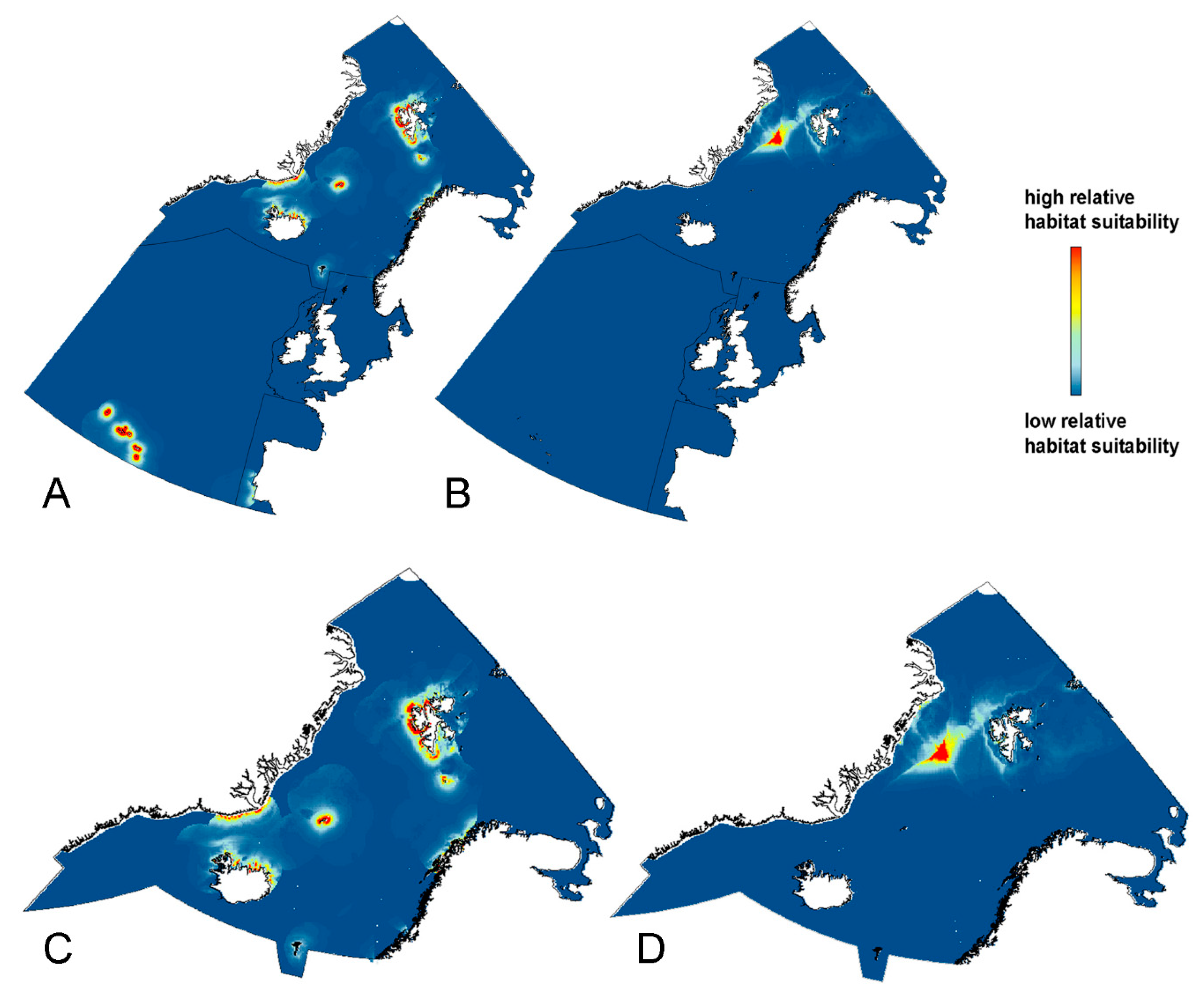
Thus, the following approach to identify species-specific areas suitable for additional MPAs within the OSPAR region was applied. The overall goal was to protect, at best, the upper 30% of the key habitats of each species. This was motivated by operational objective S5.O1. of the North-East Atlantic Environment Strategy 2030 of OSPAR, which aims to further develop its network of MPAs to cover and effectively manage at least 30% of the OSPAR maritime area by 2030 to achieve its conservation objectives.

To identify new areas suitable for additional MPAs, first the integral, ∫_all, of the predicted relative habitat suitability over the entire OSPAR area was calculated and then the same integral was calculated but only integrated over the existing MPAs (∫_all). Thus, ∫_all quantifies the overall area of key habitats in the OSPAR region, whereas ∫_all quantifies the area of key habitats within existing MPAs. Hence, the quotient of these two measures (×100) gives the percentage of species-specific key habitats that are currently protected by OSPAR MPAs.

The second step, described below, aimed to augment new areas (MPA_new), such that MPA_ex (existing MPAs) and MPA_new together cover 30% of the species-specific key habitats in the most efficient way, i.e., with a minimum required area of MPA_new. To achieve this, we stepwise augmented the 1 × 1 km pixel with the highest predicted habitat suitability value (not belonging to either MPA_ex or MPA_new) to MPA_new until the integral over MPA_ex and MPA_new reached 30% of the value ∫_all. In simple terms, the “free” pixels with the highest predicted habitat suitability are added to the proposed protected area network until 30% of the key habitat is protected.

In a third and final step (and as explained in more detail above), we reviewed and possibly modified these protected areas in light of the above points, such that at least 25% (but preferably 30%—cf., above) of the species-specific key habitats remained (cf., slight modifications for the areas proposed for the blue whale due to extrapolation errors).

3. Results

3.1. Blue Whale (Balaenoptera musculus)

Pre-selected key variables. Based on an intensive literature search in conjunction with expert communication (Supporting Material S3A), the following critical parameters were pre-selected as possible influencing factors for the blue whale: krill availability, sea surface temperature, net primary production/chlorophyll a, data on upwelling dynamics, sea ice concentration, and continental shelf slope (see Supporting Materials S3 and S4 for a more detailed motivation and derivation of these variables). Direct remote-sensing data on krill availability and/or upwelling events were not available; however, both variables can be approximated by sea surface temperature and/or chlorophyll availability, and these variables have thus been used as proxies.

Tested and selected predictor variables. The following predictors have been tested/used for the MaxEnt-based analysis: sea surface temperature, chlorophyll a, sea ice concentration, distance to the coast and water depth. The following variables remained as predictors after variable selection: distance to the nearest coast, sea surface temperature, water depth, logarithm of sea surface temperature, and logarithm of chlorophyll a.

Predicted habitats and proposed areas suitable for additional MPAs. The predicted spatial patterns of habitat suitability for blue whales are given in Figure 3A,C. Our calculations reveal that currently, 11.8% of the key habitats predicted for blue whales are already covered by the existing OSPAR MPA network. In addition, the proposed areas suitable for blue whale-specific MPAs are shown in Figure 4A. Here, we excluded only small areas with high predicted habitat suitability at the Blosseville Coast, where blue whales do not occur regularly (R. G. Hansen, pers. comm.); we ascribe this prediction error to uncertainties connected to extrapolations. As a result, instead of 30% only 28.7% protection remained.

3.2. Bowhead Whale (Balaena mysticetus)

Pre-selected key variables. Based on an extensive literature review and expert consultations (see Supporting Material S3B), the following critical parameters were pre-selected as potential influencing factors, namely sea surface temperature, (seasonal) sea ice coverage and thickness/volume, water depth, and distance to the coast, as well as salinity and current-related variables, bottom slope, human activities (namely shipping), and variables representing food availability (such as chlorophyll a). More detailed species background information and preferences are given in Supporting Materials S3 and S4.

Tested and selected predictor variables. The following predictors have finally been tested/used for variable selection during the MaxEnt-based analysis: chlorophyll a, water depth, distance to the coast, sea ice intensity, sea ice thickness, sea surface temperature, different types of sea surface currents, and vessel density. More detailed information on these variables, data sources, and transformed variants of these variables are given above and in the Supporting Material S4. The following variables remained as predictors after variable selection: the spatial gradient of the logarithm of sea ice intensity, the logarithm of water depth, the logarithm of sea ice thickness, and the spatial gradient of water depth.

Predicted habitats and identified areas suitable for additional MPAs. The predicted relative habitat suitability patterns are given in Figure 3B,D. Our calculations suggest that currently, only 4.1% of the key habitats predicted for bowheads are already covered by the existing MPA network. The identified areas suitable for bowhead whale-specific new MPAs are shown in Figure 4B. No changes in the predicted upper 30% of key habitats are suggested.

4. Discussion

The predicted distribution of relative habitat suitability within the OSPAR area with respect to the blue whale (Figure 3A) mainly concerns waters of the Svalbard archipelago, Iceland and the Azores. For the bowhead whale, the most important areas/habitats concern waters between the Svalbard archipelago and Greenland, particularly the Fram Strait (Figure 3B).

For the blue whale, this strongly coincides with the coarse distribution map provided by Carwardine [34]. In particular, the main distribution between the north-eastern coast of Iceland and the western coast of the Svalbard archipelago, but also movements as far south as the Azores [35,36]. Previous studies, however, also identified a core area for this species in waters south of Iceland [37], which is not indicated by our raw data (Figure 2) or our predicted habitat suitability (Figure 3), or by the coarse map of Carwardine [34]. This apparent discrepancy might be explained by the fact that Pike et al. [37] considered data from 1987–2001 when a distinct trend in blue whale sightings was observed, being increasingly relocated from the south of Iceland to more northern regions. A further increase in the use of northern areas could be explained and driven by individuals passing from the Pacific stock to the North Atlantic [38]. A continuation of this process may have led to the current, complete lack of individuals on the southern coast of Iceland in the data from 2000–2020, as reflected in the raw data and predictions of this study.

In further accordance with previous studies, our predictions indicated that blue whales (respectively, their key habitats) are nearly completely absent in the centre of the OSPAR area (North Sea and UK waters) [39]; non-zero predicted patterns only concern waters north of UK waters, while rare observations and strandings have been described west of Ireland in the last two decades [40,41]. Our predictions also include a hotspot at the Azores (Figure 3A, bottom) in accordance with known migration routes for this species [36,42]. However, the corresponding migration corridor between Iceland and the Azores is not reflected in the predicted map, probably due to a lack of data (M. Silva, pers. comm.). Our predicted patterns with respect to the direct surroundings of the Svalbard archipelago (Figure 3C) strongly coincide with the patterns presented in Storrie et al. [43].

In summary, the predicted key habitats for the blue whale are in accordance with previous (sparse) knowledge about key habitats and distribution patterns of this species. Key habitats are already well covered by existing MPAs around the Svalbard archipelago but MPAs are lacking north of Iceland and in the waters of the Azores. However, as detailed in the “Material and methods” section, the key habitats derived from presence-only methods might be partially confounded by the spatial pattern of survey effort (cf., Discussion below), i.e., predicted key habitats might be correspondingly biased and/or other key habitats might still be missing. In addition (probably due to lack of data), the migration corridor between Iceland and the Azores is not reflected.

With respect to the bowhead whale, no diet-specific variables were selected during the variable selection algorithm. This is most probably due to the fact that the data basis for both bowhead whales and their specific diet in Arctic waters is very sparse; significant correlations between whales and dietary variables generally require both high observation numbers (at best from systematic surveys) and the existence of variables (e.g., based on corresponding surveys) that reflect the diet to a sufficient extent (e.g., the work of Gilles et al. [44], based on 14,356 positive sightings of harbour porpoises in addition to specific survey data on sand eel (Ammodytes spp.) grounds).

The predicted overall distribution of habitat suitability of the considered subpopulation within the OSPAR area (“Spitsbergen stock”) appears to be concentrated between Greenland and the Svalbard archipelago, reaching east across the northern Barents Sea to Franz Josef Land (Figure 3B, top), altogether spanning a belt in the areas close to the Arctic ice edge, as described previously, e.g., in surveys around Svalbard [45]. Published information on the distribution of this species in the OSPAR area (or parts of the region) is sparse. However, simple (binary) maps are available. A circumpolar distribution was already presumed by, e.g., Carwardine [34] and Shirihai and Jarret [46]. The former proposes a distribution reaching down to the waters of Iceland, in contrast to Shirihai and Jarret [46], who, in accordance with our predictions, indicated regions restricted distinctly north of Iceland. Indeed, the distribution range in the binary map proposed by Reeves et al. [47] coincides well with our modelled distribution and raw data, restricting the regularly used grounds to those approximately at the latitudinal range of the Svalbard archipelago. Sightings in more temperate waters are very rare [48], which is again in accordance with our modelled distribution of key habitats.

Our predictions suggest a distinct maximum of bowhead whale habitat suitability between Greenland and the Svalbard archipelago in the region of the Fram Strait. This preference has been indicated by survey data [38,49,50] and additionally documented by tagged individuals [51]. The latter dataset was not available for our present study and may thus be considered as an independent and recent validation dataset. Although the data presented by Kovacs et al. [51] only relied on 13 individuals, they reproduced the predicted pattern in Figure 3B,D quite well. Our results thus suggest that the distinct accumulation at the Fram Strait might represent an important current area for bowheads in the OSPAR area, further supporting the observations and results of de Boer et al. [49] and Joiris [38]. However, the same restrictions, as described above for the blue whale, need to be considered when it comes to potential bias due to presence-only methods.

The recently reported potential summering ground of bowhead whales in part of the Northeast Water Polynya [52] does not appear in our modelled distribution. However, this very local concentration might be below the spatial scale of the applied modelling approach. In addition, the work of Boertmann et al. [52] was based on bowhead whale numbers strongly corrected for overseen individuals, whereas the present approach is based on raw data only. Our model predicts suitable habitats near the Svalbard archipelago but shows the highest values northwest of the archipelago—consistent with the recent observations reported by Storrie et al. [43]. The same holds for the coastal waters off northeast Greenland, where our model predictions show existent but low habitat suitability in accordance with previous sightings [53,54,55]. Results shown in this study indicate that key habitats are poorly covered with MPAs so far and suggest that additional MPAs in the Fram Strait would strongly contribute to the protection of key habitats of bowhead whales in the OSPAR maritime area.

We are aware of the legitimate criticisms of presence-only methods compared with the regression-based analysis of systematic survey data (cf. also “Material and Methods” section). However, at the scale of the modelled OSPAR area and considering these limitations, we assume (and verified) that survey data are not sufficient for reliable regression-based estimates (as, e.g., applied by Mercker et al. [8]) for the two whales considered in this study. In terms of both spatial coverage and total number of non-zero observations, the analysis of presence-only data (augmented with pseudo-absences) was therefore preferred, despite the statistical disadvantages (such as sampling bias). In addition, predicted key habitats are based on all available but not all existing data and, thus, represent neither the “true” nor the best-possible representation of key habitats, i.e., important areas might still be missing. Given the available data basis, we have, however, chosen—to the best of our knowledge—the best possible way to make valid estimates, which, in addition to many technical aspects to avoid bias, also included the above-mentioned intensive involvement of various experts for validation and plausibility checks.

Several of the final selected variables used to predict the species-specific key habitats will change over the coming years with the North Atlantic warming due to climate change, such as increased sea surface temperature, sea ice intensity, sea ice thickness, and changes in chlorophyll a distribution. Thus, together with improving data availability, our predictions should be regularly updated with respect to these expected changes—an important aspect conservation planning and MPA designation processes must take into account [56].

However, the modelling approach performed in this study presents a highly empirical approach to identifying key habitats for two endangered cetacean species: the bowhead and the blue whale. In particular, the use of all available observation data from the entire OSPAR area to predict the distribution of key habitats for each species using appropriately adapted statistical methods is considered a major advantage—in particular, in combination with intensive communication with a wide range of experts, both regarding the selection of the predictors to be considered and regarding the plausibility of the results. As a result, this study identified regions that are highly suitable for additional MPAs, which could increase the protection of key habitats for the two species as efficiently as possible. For the blue whale, this primarily concerns the waters around the Azores, and for the bowhead whale, the region around the Fram Strait. We, therefore, recommend that both areas should be considered as additional MPAs to strengthen the protection of these species in the context of the Regional Seas Convention OSPAR.

5. Summary and Outlook

By using a modelling approach, this study identified suitable areas for MPAs to effectively protect bowhead and blue whales in the OSPAR area. To achieve this goal, we aimed to acquire as much species data as possible and applied suitable modelling techniques for the available (sparse) data situation in interplay with various expert knowledge and previously published data. Thus, evidence-based and expert-validated proposals for new MPAs are presented to increase MPA coverage in the most efficient way for two threatened, highly mobile and data-poor cetacean species within the OSPAR maritime area.

This information can serve as a valuable basis for discussions about the selection of areas for new MPAs within OSPAR to reach policy goals and enhance the protection of the considered species in the North-East Atlantic. Efforts should be made by OSPAR to implement the findings and designate new MPAs, as well as to improve data availability through intensified survey and monitoring activities.

In particular, this study suggests that waters north of Iceland and around the Azores should be better protected for the blue whale, and areas in the Fram Strait region should be protected for the bowhead whale. In addition, it would be highly desirable to intensify systematic surveys to obtain better data on the distribution of those species in the OSPAR area—particularly concerning regular marine mammal surveys in the northern half of the OSPAR convention area, where those data are still largely lacking.

The presented methods and results can help to come a step closer to the “30 × 30 goal” in an empirically and scientifically sound way and thus contribute to tackling one of the greatest challenges of our time: species protection despite the major upheavals in the marine environment due to human activities and climate change.

References

1. OSPAR, 2022. OSPAR Convention for the Protection of the Marine Environment of the North-East Atlantic. OSPAR Commission. Available online: https://www.ospar.org/convention (accessed on 7 February 2022).
2. Hooker, S.K.; Canadas, A.M.; Hyrenbach, K.D.; Corrigan, C.; Polovina, J.J.; Reeves, R.R. Making Protected Area Networks Effective for Marine Top Predators. Endanger. Species Res. 2011, 13, 203–218. [Google Scholar] [CrossRef]
3. Hoyt, E. Marine Protected Areas for Whales, Dolphins and Porpoises: A World Handbook for Cetacean Habitat Conservation and Planning; Earthscan: Oxford, UK; Routledge: London, UK; Taylor & Francis: New York, NY, USA, 2011. [Google Scholar]
4. Reeves, R.R. Dolphins, Whales, and Porpoises: 2002–2010 Conservation Action Plan for the World’S…: 2002–2010 Conservation Action Plan for the World’s Cetaceans, 2nd ed.; Union Internationale pour la Conservation de la Nature et de ses Ressources: Gland, Switzerland; Cambridge, UK, 2003; ISBN 978-2-8317-0656-6. [Google Scholar]
5. OSPAR MPAs. Available online: http://mpa.ospar.org/home_ospar (accessed on 13 May 2023).
6. OSPAR List of Threatened and/or Declining Species and Habitats. Available online: https://www.ospar.org/work-areas/bdc/species-habitats/list-of-threatened-declining-species-habitats (accessed on 23 February 2023).
7. POSH Roadmap. Available online: https://www.ospar.org/news/implementing-collective-actions-on-threatened-and-or-declining-species (accessed on 23 June 2023).
8. Mercker, M.; Markones, N.; Borkenhagen, K.; Schwemmer, H.; Wahl, J.; Garthe, S. An Integrated Framework to Estimate Seabird Population Numbers and Trends. J. Wildl. Manag. 2021, 85, 751–771. [Google Scholar] [CrossRef]
9. Merow, C.; Smith, M.J.; Silander, J.A., Jr. A practical guide to MaxEnt for modeling species’ distributions: What it does, and why inputs and settings matter. Ecography 2013, 36, 1058–1069. [Google Scholar] [CrossRef]
10. Korner-Nievergelt, F.; Roth, T.; von Felten, S.; Guelat, J.; Almasi, B.; Korner-Nievergelt, P. Bayesian Data Analysis in Ecology Using Linear Models with R, BUGS, and Stan; Elsevier: London, UK, 2015. [Google Scholar]
11. Wood, S. Generalized Additive Models: An Introduction with R; Chapman & Hall/CRC: Boca Raton, FL, USA, 2017. [Google Scholar]
12. Zuur, A.; Ieno, E.; Smith, G.M. Analysing Ecological Data; Springer Science+Business Media, LLC: Berlin/Heidelberg, Germany, 2007. [Google Scholar]
13. Zuur, A.F.; Ieno, E.N.; Saveliev, A.A. Spatial, Temporal and Spatial-Temporal Ecological Data Analysis with R-INLA, Volume I–II; Highland Statistics Ltd.: Newburgh, UK, 2017. [Google Scholar]
14. Gilles, A.; Authier, M.; Ramirez-Martinez, N.; Araújo, H.; Blanchard, A.; Carlström, J.; Eira, C.; Dorémus, G.; Fernández-Maldonado, C.; Geelhoed, S.C.V.; et al. Scans-IV. Small Cetaceans in Euopean Atlantic Water and the North Sea 2022. In Proceedings of the 34th Annual Conference of the European Cetacean Society, O Grove, Spain, 16–20 April 2023. [Google Scholar]
15. Philipps, S.J.; Dudik, M. Modeling of Species Distributions with Maxent: New Extensions and a Comprehensive Evaluation. Ecography 2008, 31, 161–175. [Google Scholar]
16. Elith, J.; Hastie, T.; Dudik, M.; Chee, Y.; Yates, C.J.; Phillips, S.J. A Statistical Explanation of MaxEnt for Ecologists. Divers. Distrib. 2011, 17, 43–57. [Google Scholar]
17. Bost, C.A.; Cotté, C.; Bailleul, F.; Cherel, Y.; Charrassin, J.B.; Guinet, C.; Ainley, D.G.; Weimerskirch, H. The Importance of Oceanographic Fronts to Marine Birds and Mammals of the Southern Oceans. J. Mar. Syst. 2009, 78, 363–376. [Google Scholar] [CrossRef]
18. Schneider, D.C. Seabirds and Fronts: A Brief Overview. Polar Res. 1990, 8, 17–21. [Google Scholar] [CrossRef]
19. Renner, I.W.; Elith, J.; Fithian, W.; Hastie, T.; Phillips; Warton, D.I.; Baddeley, A.; Popovic, G. Point Process Models for Presence-Only Analysis. Methods Ecol. Evol. 2015, 6, 366–379. [Google Scholar]
20. Renner, I.W.; Warton, D.I. Equivalence of MAXENT and Poisson Point Process Models for Species Distribution Modeling in Ecology. Biometrics 2013, 69, 274–281. [Google Scholar] [CrossRef]
21. Fourcade, Y.; Engler, J.O.; Rödder, D.; Secondi, J. Mapping Species Distributions with MAXENT Using a Geographically Biased Sample of Presence Data: A Performance Assessment of Methods for Correcting Sampling Bias. PLoS ONE 2014, 9, e97122. [Google Scholar] [CrossRef]
22. Botella, C.; Joly, A.; Monestiez, P.; Bonnet, P.; Munoz, F. Bias in Presence-Only Niche Models Related to Sampling Effort and Species Niches: Lessons for Background Point Selection. PLoS ONE 2020, 15, e0232078. [Google Scholar] [CrossRef]
23. Ready, J.; Kaschner, K.; South, A.B.; Eastwood, P.D.; Rees, T.; Rius, J.; Agbayani, E.; Kullander, S.; Froese, R. Predicting the Distributions of Marine Organisms at the Global Scale. Ecol. Model. 2010, 221, 467–478. [Google Scholar] [CrossRef]
24. Vollering, J.; Halvorsen, R.; Mazzoni, S. The MIAmaxent R Package: Variable Transformation and Model Selection for Species Distribution Models. Ecol. Evol. 2019, 9, 12051–12068. [Google Scholar] [CrossRef]
25. R Core Team. R: A Language and Environment for Statistical Computing; R Foundation for Statistical Computing: Vienna, Austria, 2024; Available online: https://www.R-project.org (accessed on 5 February 2024).
26. Wickham, H. Ggplot2: Elegant Graphics for Data Analysis; Springer: New York, NY, USA, 2009. [Google Scholar]
27. Hijmans, R.J. Raster: Geographic Data Analysis and Modeling. R Package Version 2.5-8. 2016. Available online: https://cran.r-project.org/web/packages/raster/raster.pdf (accessed on 15 March 2023).
28. Hijmans, R.J.; van Etten, J. Raster: Geographic Analysis and Modeling with Raster Data. R Package Version 2.0-12. 2012. Available online: http://CRAN.R-project.org/package=raster (accessed on 15 March 2023).
29. Pebesma, E. Simple Features for R: Standardized Support for Spatial Vector Data. R J. 2018, 10, 439–446. [Google Scholar]
30. Baddeley, A.; Turner, R. spatstat: An R Package for Analyzing Spatial Point Patterns. J. Stat. Softw. 2005, 12, 1–42. [Google Scholar] [CrossRef]
31. Grolemund, G.; Wickham, H. Dates and Times Made Easy with Lubridate. J. Stat. Softw. 2011, 40, 1–25. [Google Scholar] [CrossRef]
32. Arya, S.; Kemp, S.E.; Jefferis, G. Mount RANN: Fast Nearest Neighbour Search (Wraps ANN Library) Using L2 Metric 2019. Available online: https://jefferislab.r-universe.dev/RANN (accessed on 12 August 2024).
33. Wickham, H. The Split-Apply-Combine Strategy for Data Analysis. J. Stat. Softw. 2011, 40, 1–29. [Google Scholar] [CrossRef]
34. Carwardine, M. Handbook of Whales, Doplhins, and Porpoises of the World; Princeton University Press: Princeton, NJ, USA; Oxford, UK, 2020. [Google Scholar]
35. OSPAR Biodiversity Committee Assessments—Status. 2020. Available online: https://oap.ospar.org/en/ospar-assessments/committee-assessments/biodiversity-committee/status-assesments/blue-whale/ (accessed on 15 March 2023).
36. Silva, M.A.; Prieto, R.; Jonsen, I.; Baumgartner, M.F.; Santos, R.S. North Atlantic Blue and Fin Whales Suspend Their Spring Migration to Forage in Middle Latitudes: Building up Energy Reserves for the Journey? PLoS ONE 2013, 8, e76507. [Google Scholar] [CrossRef]
37. Pike, D.G.; Víkingsson, G.A.; Gunnlaugsson, T.; Øien, N. A Note on the Distribution and Abundance of Blue Whales (Blalaenoptera musculus) in the Central and Northeast North Atlantic. NAMMCO Sci. Entific. Publ. 2009, 7. [Google Scholar] [CrossRef]
38. Joiris, C.R. Considerable Increase in Bowhead, Blue, Humpback and Fin Whales Numbers in the Greenland Sea and Fram Strait between 1979 and 2014. Adv. Polar Sci. 2016, 2, 117–125. [Google Scholar]
39. OSPAR Abundance and Distribution of Cetaceans—Sheet Reference: BDC15/D103 2018. Available online: https://oap.ospar.org/en/ospar-assessments/intermediate-assessment-2017/biodiversity-status/marine-mammals/abundance-distribution-cetaceans/abundance-and-distribution-cetaceans/ (accessed on 11 August 2024).
40. Reid, J.B.; Evans, P.G.H.; Northridge, S.P. Atlas of Cetacean: Distribution in North-West European Waters; Joint Nature Conservation Committee: Peterborough, UK, 2003.
41. Wall, D.; O’kelly, I.; Whooley, P.; Tyndall, P. New records of blue whales (Balaenoptera musculus) with evidence of possible feeding behaviour from the continental shelf slopes to the west of Ireland. Mar. Biodivers. Rec. 2009, 2, e128. [Google Scholar] [CrossRef]
42. Visser, F.; Hartman, K.L.; Pierce, G.J.; Valavanis, V.D.; Huisman, J. Timing of Migratory Baleen Whales at the Azores in Relation to the North Atlantic Spring Bloom. Mar. Ecol. Prog. Ser. 2011, 440, 267–279. [Google Scholar] [CrossRef]
43. Storrie, L.; Lydersen, C.; Andersen, M.; Wynn, R.B.; Kovacs, K.M. Determining the Species Assemblage and Habitat Use of Cetaceans in the Svalbard Archipelago, Based on Observations from 2002 to 2014. Polar Res. 2018, 37, 1463065. [Google Scholar] [CrossRef]
44. Gilles, A.; Viquerat, S.; Becker, A.A.; Forney, K.A.; Geelhoed, S.C.V.; Helters, J.; Nabe-Nielsen, J.; Scheidat, M.; Siebert, U.; Sveegard, S.; et al. Seasonal habitat-based density models for a marine top predator, the harbor porpoise, in a dynamic environment. Ecosphere 2016, 7, e01367. [Google Scholar]
45. Vacquié-Garcia, J.; Lydersen, C.; Marques, T.A.; Aars, J.; Ahonen, H.; Skern-Mauritzen, M.; Øien, N.; Kovacs, K.M. Late Summer Distribution and Abundance of Ice-Associated Whales in the Norwegian High Arctic. Endanger. Species Res. 2017, 32, 59–70. [Google Scholar] [CrossRef]
46. Shirihai, H.; Jarret, B. Whales, Dolphins And Seals: A Field Guide to the Marine Mammals of the World; A & C Black: London, UK, 2006. [Google Scholar]
47. Reeves, R.R.; Ewins, P.J.; Agbayani, S.; Heide-Jørgensen, M.P.; Kovacs, K.M.; Lydersen, C.; Suydam, R.; Elliott, W.; Polet, G.; van Dijk, Y.; et al. Distribution of Endemic Cetaceans in Relation to Hydrocarbon Development and Commercial Shipping in a Warming Arctic. Mar. Policy 2014, 44, 375–389. [Google Scholar] [CrossRef]
48. de Boer, M.N.; Jones, D.; Jones, H. Ocean Wanderers: Extralimital Encounters with Bowhead Whales (Balaena mysticetus) in Temperate European Shallow Waters. Aquat. Mamm. 2017, 43, 279–288. [Google Scholar] [CrossRef]
49. de Boer, M.N.; Janinhoff, N.; Nijs, G.; Verdaat, H. Encouraging Encounters: Unusual Aggregations of Bowhead Whales Balaena mysticetus in the Western Fram Strait. Endanger. Species Res. 2019, 39, 51–62. [Google Scholar] [CrossRef]
50. Wiig, Ø.; Bachmann, L.; Kovacs, K.; Swift, R.; Lydersen, C. Survey of Bowhead Whales (Balaena mysticetus) in the Northeast Atlantic in 2010. 2010. Available online: https://www.researchgate.net/publication/242579602_Survey_of_bowhead_whales_Balaena_mysticetus_in_the_Northeast_Atlantic_in_2010 (accessed on 15 March 2023).
51. Kovacs, K.M.; Lydersen, C.; Vacquiè-Garcia, J.; Shpak, O.; Glazov, D.; Heide-Jørgensen, M.P. The Endangered Spitsbergen Bowhead Whales’ Secrets Revealed after Hundreds of Years in Hiding. Biol. Lett. 2020, 16, 20200148. [Google Scholar] [CrossRef]
52. Boertmann, D.; Kyhn, L.A.; Witting, L.; Heide-Jørgensen, M.P. A hidden getaway for bowhead whales in the Greenland Sea. Polar Biol. 2015, 38, 1315–1319. [Google Scholar] [CrossRef]
53. Boertmann, D.; Merkel, F.; Durinck, J. Bowhead Whales in East Greenland, Summers 2006–2008. Polar Biol. 2009, 32, 1805–1809. [Google Scholar] [CrossRef]
54. Boertmann, D.; Nielsen, R.D. A bowhead whale calf observed in northeast Greenland waters. Polar Rec. 2010, 46, 373–375. [Google Scholar] [CrossRef]
55. Gilg, O.; Born, E.W. Recent Sightings of the Bowhead Whale (Balaena mysticetus) in Northeast Greenland and the Greenland Sea. Polar Biol. 2005, 28, 796–801. [Google Scholar] [CrossRef]
56. Lee, H.; Irvine, A.; Brito-Morales, I.; Fuller, S.; Davies, T.; Tittensor, D.; Reville, G.; Shackell, N.; Hennicke, J.; Stanley, R. To Save the High Seas, Plan for Climate Change. Nature 2024, 630, 298–301. [Google Scholar]
57. ESAS. Available online: https://www.ices.dk/data/data-portals/Pages/European-Seabirds-at-sea.aspx (accessed on 5 June 2022).
58. SCANS-III. Available online: https://scans3.wp.st-andrews.ac.uk/ (accessed on 1 May 2024).
59. GBIF. Available online: https://www.gbif.org/ (accessed on 1 May 2024).
60. Norwegian Biodiversity Centre & Polar Institute: Arctic Data. Available online: https://www.npolar.no/ (accessed on 1 March 2023).
61. Kovacs, K.M.; Andersen, M. Marine Mammals Sightings in and around Svalbard 1995–2019 [Data Set]. Available online: https://data.npolar.no/dataset/246c1053-6fdc-5043-b7b4-284f4fa8c095 (accessed on 11 August 2024).
62. Artsdatenbanken/Norwegian Biodiversity Centre Map Service. Available online: https://artsdatabanken.no/ (accessed on 3 May 2022).
63. OBIS. Available online: https://obis.org/ (accessed on 3 June 2022).
64. Vertnet. Available online: http://vertnet.org/ (accessed on 1 June 2022).
65. RusMam. Available online: https://rusmam.ru/atlas/map (accessed on 3 May 2022).
66. OSPAR Case Reports for the OSPAR List of Threatened and/or Declining Species and Habitats. 2008. Available online: https://qsr2010.ospar.org/media/assessments/p00358_case_reports_species_and_habitats_2008.pdf (accessed on 11 August 2024).
67. OSPAR Background Document for Blue Whale: Balaenoptera musculus. 2010. Available online: https://www.ospar.org/documents?d=7232 (accessed on 11 August 2024).
68. Lesage, V.; Gosselin, J.-F.; Lawson, J.W.; McQuinn, I.; Moors-Murphy, H.; Plourde, S.; Sears, R.; Simard, Y. Habitats Important to Blue Whales (Balaenoptera musculus) in the Western North Atlantic; Canadian Science Advisory Secretariat (CSAS): Ottawa, ON, USA, 2018; pp. 1–56. [Google Scholar]
69. Barlow, D.R.; Torres, L.G. Planning Ahead: Dynamic Models Forecast Blue Whale Distribution with Applications for Spatial Management. J. Appl. Ecol. 2021, 58, 2493–2504. [Google Scholar] [CrossRef]
70. George, J.C.; Theweissen, J.G.M. The Bowhead Whale: Balaena mysticetus: Biology and Human Interactions; Academic Press Inc.: London, UK, 2021. [Google Scholar]
71. Citta, J.J.; Quakenbush, L.T.; Okkonen, S.R.; Druckenmiller, M.L.; Maslowski, W.; Clement-Kinney, J.; George, J.C.; Brower, H.; Small, R.J.; Ashjian, C.J.; et al. Ecological Characteristics of Core-Use Areas Used by Bering–Chukchi–Beaufort (BCB) Bowhead Whales, 2006–2012. Prog. Oceanogr. 2015, 136, 201–222. [Google Scholar] [CrossRef]
72. Harwood, L.A.; Quakenbush, L.T.; Small, R.J.; George, J.C.; Pokiak, J.; Pokiak, C.; Heide-Jørgensen, M.P.; Lea, E.V.; Brower, H. Movements and Inferred Foraging by Bowhead Whales in the Canadian Beaufort Sea during August and September, 2006–12. Arctic 2017, 70, 161–176. [Google Scholar] [CrossRef]
73. Citta, J.J.; Okkonen, S.R.; Quakenbush, L.T.; Maslowski, W.; Osinski, R.; George, J.C.; Small, R.J.; Brower, H.; Heide-Jørgensen, M.P.; Harwood, L.A. Oceanographic Characteristics Associated with Autumn Movements of Bowhead Whales in the Chukchi Sea. Deep. Sea Res. Part II Top. Stud. Oceanogr. 2018, 152, 121–131. [Google Scholar] [CrossRef]
74. Chambault, P.; Albertsen, C.M.; Patterson, T.A.; Hansen, R.G.; Tervo, O.; Laidre, K.L.; Heide-Jørgensen, M.P. Sea Surface Temperature Predicts the Movements of an Arctic Cetacean: The Bowhead Whale. Sci. Rep. 2018, 8, 9658. [Google Scholar] [CrossRef]
75. CLS Maritime Intelligence. Available online: https://maritime-intelligence.groupcls.com/ (accessed on 1 June 2023).
76. NASA Ocean Color Web—Distcoast. Available online: https://oceancolor.gsfc.nasa.gov/resources/docs/distfromcoast/ (accessed on 2 June 2022).
77. NASA AQUA MODIS Web. Available online: https://neo.gsfc.nasa.gov/view.php?datasetId=MYD28M (accessed on 6 August 2022).
78. Marine Conservation Institute (MCI). Available online: https://www.arcgis.com/home/item.html?id=ab0926890e444fd0a2ecd4f40fb318f7 (accessed on 8 August 2023).
79. NASA Ocean Color Web-Chorophyll a. Available online: https://oceancolor.gsfc.nasa.gov/resources/atbd/chlor_a/ (accessed on 8 August 2022).
80. GEBCO Compilation Group (2020) GEBCO 2020 Grid. Doi:10.5285/A29c5465-B138-234d-E053-6c86abc040b9. Available online: https://www.gebco.net/data_and_products/gridded_bathymetry_data/ (accessed on 8 August 2022).
81. Global SMOS Level 4 Sea Surface Salinity File (Institution: Barcelona Expert Center (BEC)). Available online: https://erddap.emodnet.eu/erddap/index.html (accessed on 7 August 2022).
82. National Snow and Ice Data Center Respectively NOAA. Available online: https://nsidc.org/data/seaice_index (accessed on 5 August 2022).
83. Yi, D.; Zwally, H.J. Arctic Sea Ice Freeboard and Thickness; Version 1; Updated 2014-04-15; NASA National Snow and Ice Data Center Distributed Active Archive Center: Boulder, CO, USA, 2009. [Google Scholar]
84. Swedish National Data Service (SND). Dataset. (Obst, M. (2017). Global Tidal Variables (1.0). University of Gothenburg. Available online: https://snd.gu.se/en/catalogue/study/ecds0243# (accessed on 5 August 2022).
Figure 1. Schematic overview of tasks and workflow of the present study.
Jmse 12 01445 g001
Figure 2. Count (left) and presence-only (right) data for blue and bowhead whales. Red dots represent positive counts, and blue dots represent zero counts. “N_total” indicates the overall number of (zero or positive) observations, and “N_obs” indicates the total number of positive observations only.
Jmse 12 01445 g002
Figure 3. MaxEnt-based predicted relative habitat suitability (heatmap colour scale) for blue whales (Balaenoptera musculus) (A,C) and bowheads (Balaena mysticetus) (B,D) for all sexes and ages in the entire OSPAR area (A,B) and the northern subregion I (C,D) comprising arctic waters. Warm colours correspond to high relative habitat suitability, whereas cold colours correspond to low corresponding values.
Jmse 12 01445 g003
Figure 4. Identified locations suitable for new MPAs (red coloured) augmenting existing MPAs (grey) considering protection of blue whales (A), respectively, the bowhead (C). For visualisation purposes, the OSPAR area (C) is in (A,B) cropped to the subregion where proposed MPAs occur for each considered species. (B) is taken and modified with kind permission from the Federal Agency for Nature Conservation (BfN).
Jmse 12 01445 g004
Disclaimer/Publisher’s Note: The statements, opinions and data contained in all publications are solely those of the individual author(s) and contributor(s) and not of MDPI and/or the editor(s). MDPI and/or the editor(s) disclaim responsibility for any injury to people or property resulting from any ideas, methods, instructions or products referred to in the content.