A New Perspective of the Spring Predictability Barrier Based on the Zonal Sea Level Pressure Gradient

Abstract

Currently, the “spring predictability barrier” (SPB) is still a controversial problem in many atmosphere–ocean coupled models and has significant impacts on degrading the El Niño–Southern Oscillation (ENSO) predictions across the boreal spring. In this study, unlike previous studies that viewed the SPB issue from the perspective of sea surface temperature (SST), based on the Bjerknes feedback theory and the decadal variations in Walker circulation over the tropical Pacific, a new perspective of the SPB is revealed by the seasonal variations in the observed zonal sea level pressure (SLP) gradient, which can reflect the stability and variability of the atmosphere–ocean interactions during the ENSO’s evolution. More importantly, a significant decadal variation of SPB strength (SPBS) is exhibited in the last 3 decades, from 1991 to 2020, which is strongly controlled by the dominant patterns of sea surface temperature (SST) and Walker circulation, and associated with the background mean atmosphere–ocean states. That is to say, the atmosphere–ocean interaction pattern over the tropical Pacific has undergone decadal variations over the past 3 decades which determine the decadal variations in SPBS. International Research Institute for Climate and Society/Climate Prediction Center (IRI/CPC) multi-models show stronger SPBS during 2001–2010 than during 2011–2020, indicating that the decadal variations in SPBS from statistical analysis also exist in actual model predictions, which further confirms the rationality of this perspective of SPB based on the zonal SLP gradient.

1. Introduction

El Niño–Southern Oscillation (ENSO) is one of the most important sources of climate variability on the seasonal to interannual timescales and has been extensively studied in the past few decades. Since the Zebiak–Cane (ZC) model first reproduced the main observed features of ENSO [1], models with various complexities of atmosphere–ocean coupling have been developed to simulate and predict ENSO events. The state-of-the-art coupled models have reached a stage at which accurate predictions can be made 6–12 months in advance [2,3,4,5,6,7,8,9]. However, the “spring predictability barrier” (SPB) problem, which refers to a sudden decline of the prediction skill in the boreal spring [10], remains in many models and significantly exists in sea surface temperature (SST) prediction [11,12,13]. Recent reviews indicate that, regardless of the complexity of the model, this strong seasonal variation in the forecast skill is a common feature of statistical and dynamical models [2,5,14,15,16,17].

It should be noted that, corresponding to this predictability-oriented SPB definition, a similar phenomenon also exists but regarding to the persistence forecast, which is a simple type of climate forecast that requires only knowledge of current conditions to forecast conditions in the coming months. In particular, it reveals that the persistence of the ENSO signal shows a significant decrease across the boreal spring, which is termed as the spring persistence barrier, with the same abbreviation of SPB [17,18,19,20,21]. Actually, this persistence-oriented SPB definition is highly synchronized with the predictability-oriented one, since they are both regulated by the physical relationships governed by the strong atmosphere–ocean coupling over the tropical Pacific region [18,19,22,23]. As a result, investigating the physical reasons inducing the persistence-oriented SPB is also an important and effective way to settle the renowned predictability-oriented SPB matter.

On the view of the decadal timescale, ENSO forecast skills were noticed to significantly decline around and since the year 2000 [8,24,25,26,27], when a shift in the climate took place in the tropical Pacific that was characterized by a dramatic La Niña-like background pattern and enhanced trade winds [28,29,30]. Corresponding to this abrupt variation, whether a significant climate shift in SPB occurred needs to be further explored. Moreover, it has been reported that the SPB strength (SPBS) also showed a decadal variation in the past several decades [20,21,31,32,33,34], but the hidden mechanism remains unclear. In view of this, if there is a reasonable index that can reflect SPBS, it will be of positive help for us to study the above issues. Although some previous studies have attempted to define the SPB index [34,35], they were mostly based on the perspective of sea surface temperature (SST). In this work, the seasonal variations in the observed zonal sea level pressure (SLP) gradient over the equatorial Pacific, as originated from the variability of the Walker circulation in different seasons, are adopted to explore a new perspective of the SPB. Our results confirm that SPBS did undergo a shift around the year 2000. Moreover, in line with the decadal variations of the dominant type of ENSO and corresponding atmosphere–ocean interaction during the past 3 decades (1991–2020), significant decadal shifts of SPBS are also found on the proposed SPB aspect by the zonal SLP gradient. That is, the SPBS significantly increased in the 2000s compared to the 1990s, but weakened again in the 2010s.

2. Datasets and Methods

2.1. Datasets

In this work, the Southern Oscillation Index (SOI), which is defined by the differences between the standardized SLP averaged over Indonesia (90°–140° E, 5°S–5° N) and the Equatorial Eastern Pacific (EEP; 80°–130° W, 5° S–5° N), was adopted to manifest the largescale variations over the tropical Pacific and to investigate the perspective of SPB. The monthly mean SST data used in this study were from the Hadley Centre Sea Ice and Sea Surface Temperature (HadISST) [36], which has a 1° × 1° resolution and is available from 1850 onward (http://hadobs.metoffice.com/hadisst/data/download.html accessed on 10 July 2024). Data from 1991 to 2020 was used for investigation.

The monthly mean atmospheric data include the U-wind that extends from 1000 to 10 mb with 17 vertical pressure levels, the vertical velocity (omega) that extends from 1000 to 100 mb with 12 vertical pressure levels, and the sea level pressure. They are all from the National Centers for Environmental Prediction (NCEP)/National Center for Atmospheric Research (NCAR) Reanalysis 1 dataset [37], with a 2.5° × 2.5° horizontal resolution (https://www.esrl.noaa.gov/psd/data/gridded/data.ncep.reanalysis.html accessed on 10 July 2024).

The analysis period for Niño3.4 (120°–170° W, 5° S–5° N) index, IPO (Tripole Index for the Interdecadal Pacific Oscillation) index [38], and standardized SLP over Indonesia and the EEP were all from 1986 to 2022. The Nino3.4 and IPO indices were downloaded from https://www.esrl.noaa.gov/psd/data/climateindices/list/ (accessed on 10 July 2024); SLP datasets (downloaded from http://www.cpc.ncep.noaa.gov/data/indices/ accessed on 10 July 2024) were from NOAA Climate Prediction Center (CPC).

2.2. Methods

To reveal the seasonal variations of the atmosphere–ocean interaction over the tropical Pacific, the whole period of 1991–2022 was firstly used to calculate the correlation coefficient between the SLP averaged over Indonesia and the EEP. This calculation was also adopted to 3 decades (i.e., 1991–2000, 2001–2010, and 2011–2020) to illustrate the decadal variations in SPBS. At the same time, leave-one-out cross-validation was used to estimate the range of the correlation coefficient. Leave-one-out cross-validation involves using one observation as the validation set and the remaining observations as the training set. This is repeated on all ways to cut the original sample on a validation set of one observation and a training set [39].

To illustrate the atmosphere–ocean coupling variations in the past 3 decades, multivariate EOF analysis (MEOF) was performed on the atmospheric circulation fields (U wind and omega wind) and tropical Pacific SST. When conducting EOF analysis, not only do we need to study the spatio-temporal characteristics of a certain variable, but also sometimes we need analyze a certain phenomenon, which often cannot be represented by a single variable. In this case, we need to perform EOF analysis on the combined fields of multiple variables, which is called multivariate EOF (MEOF) decomposition. In this study, MEOF was performed on the atmospheric circulation fields (U wind and omega wind) and tropical Pacific SST to obtain the dominant spatial pattern of atmosphere–ocean coupling over the tropical Pacific during different decades and to explain the reasons for the decadal variations of SPBS. Details of the MEOF analysis can be found in [40]. In this article, the March–April–May (MAM) was defined as the boreal spring. The MAM correlation between the SLP averaged over Indonesia and the EEP was defined as an SPB index.

3. The Seasonal and Decadal Perspectives of SPB According to the Variability of Zonal SLP Gradient Over Equatorial Pacific

3.1. A New SPB Index

As one of the most prominent characteristics of ENSO, a robust seasonal phase locking exists during its evolutions. That is, the SST signal over the central and eastern Pacific region always starts to appear at the boreal spring, and then develops rapidly during summer and autumn until its peak at winter, and after then the signal quickly decays to a neutral or a La Niña state [41,42]. As a result, the strongest (weakest) signal of the ENSO SST exists during the boreal winter (spring), which is well reflected by the seasonal variation of the standard deviation of the Niño3.4 SST index (a common metric of ENSO; Figure 1). Based on this reason, the other signals (noise to ENSO) are most probable and effective to contaminate the ENSO signal and lead to the least signal-to-noise ratio during the year, making the ENSO signal hardest be correctly detected and predicted during the boreal spring, i.e., the SPB phenomenon [23,43].

From the physical view, many studies have documented that the SPB is induced by the seasonal variation of the atmosphere–ocean interaction, i.e., it exhibits most weakly during the boreal spring [12,22,23,41,44,45,46,47,48,49]. As one of the most prominent engines of atmospheric circulation, the intertropical convergence zone (ITCZ) over the eastern tropical Pacific is located north of the equator all through the year, strengthening the southeast trade wind over the eastern equatorial Pacific and cooling down the SST there via the strengthening of the upwelling and local meridional overturning. This leads to a zonal contrast in the SST between the western (warm pool) and eastern Pacific (cold tongue). Low atmospheric pressure tends to occur over the warm pool, where air is heated to rise, while high pressure occurs over the cold tongue region, where air is cooled to sink. The zonal SLP gradient then forces the easterly at the sea surface, which on the one hand pushes the surface warm water to the western Pacific, while on the other hand induces the Ekman upwelling over the eastern Pacific that entrains the cold water underneath into the surface to compensate the ran out warm water [50,51]. These positive feedbacks constitute the main framework of the mean state atmosphere–ocean coupling system over the tropical Pacific region. During the boreal spring, when the ITCZ is located at its most southern position, i.e., near the equator, the induced southeast wind and upwelling is weak. This warms up the cold tongue and weakens the zonal SST contrast, which then leads to the weak zonal SLP gradient, inducing the weak easterly and upwelling over the cold tongue [52,53]. As a result, the mean state over the tropical Pacific shows the weakest atmosphere–ocean interaction during the year (Figure 1a). The blue line in Figure 1a shows the seasonal variations of the correlation coefficients between the equatorial east and west Pacific SLP anomaly, which can reflect the seasonal changes of the zonal gradient of SLP over the equatorial Pacific. It can be seen that the weakest correlation is in spring, in line with the minimum standard deviation of the Niño3.4 SST index (green line) in the same season. This reflects the weakening of the sea surface temperature contrast between the East and West Pacific in spring, resulting in the weakest atmosphere–ocean interaction and the minimum SLP gradient [52,54,55] corresponding to the ENSO SPB phenomenon.

Bjerknes pointed out that an initial positive SST anomaly in the equatorial eastern Pacific reduces the east–west SST gradient and hence weakens the Walker circulation, which results in weaker trade winds over the tropical Pacific. The weaker trade winds further drive oceanic processes to reinforce the SST anomaly. This positive atmosphere–ocean loop is then called the Bjerknes feedback, which is the most important process for the development of the ENSO events [56]. Since the strength of the atmosphere–ocean coupling during the boreal spring is weak, the SST signal over the eastern equatorial Pacific is hard to evolve and easy to be interrupted by other physical processes (i.e., noises to ENSO) [23,43]. As a result, the correlation coefficient between the SLP averaged over the western and eastern equatorial Pacific during the boreal spring could effectively reflect the weak atmosphere–ocean coupling strength and is a direct physical measurement used to investigate the SPB issue.

Regarding the significant climate shift that occurred around the year 2000, Figure 1b shows the seasonal correlation coefficients between the SLP averaged over Indonesia and the EEP during 1991–2000 and 2001–2010. It can be seen that an expected difference exists in the boreal spring between these two periods, i.e., the correlation during 1991–2000 is much clearer than that during 2001–2010 (even being a weak positive correlation). This indicates that the Walker circulation and the atmosphere–ocean coupling in the boreal spring during 1991–2000 is significantly stronger than that during 2001–2010, probably indicating a much stronger SPB happened during the latter decade. As a result, investigating the decadal variations of the correlation coefficients between the east and west SLP during the boreal spring is an effective way to understand the SPB issue. As a measurement, a new SPB index is defined in this article, which is the spring (March–April–May, MAM) mean correlation coefficient between the SLP averaged over the Indonesia and EEP regions.

Figure 1. (a) The seasonal correlation coefficients between the SLP averaged over Indonesia and the EEP during 1991–2020 (blue line) and the seasonal standard deviation of the Niño3.4 SST (green line), and (b) the seasonal correlation coefficients between the SLP averaged over Indonesia and the EEP during 1991–2000 (blue line) and 2001–2010 (cyan line). Shading indicates the range of maximum and minimum correlation coefficients from the leave-one-out cross-validation, and the dashed line shows that the correlation coefficients are significant ant the 95% confidence level.

Figure 1. (a) The seasonal correlation coefficients between the SLP averaged over Indonesia and the EEP during 1991–2020 (blue line) and the seasonal standard deviation of the Niño3.4 SST (green line), and (b) the seasonal correlation coefficients between the SLP averaged over Indonesia and the EEP during 1991–2000 (blue line) and 2001–2010 (cyan line). Shading indicates the range of maximum and minimum correlation coefficients from the leave-one-out cross-validation, and the dashed line shows that the correlation coefficients are significant ant the 95% confidence level.

3.2. Decadal Variation of SPBS and Its Physical Reasons

Figure 1b shows a significant decadal shift in SPBS around 2000. Quantitatively, we can study the changes in SPBS over the last few decades. Using the same method as in [34], Figure 2b shows the SPB index with a 10-year moving window for 1986–2022. It exhibits a significant decadal variation, with weak SPBS (large negative correlation coefficients) during the 1990s and strong one (small negative or positive correlation coefficients) during the 2000s. This is consistent with the decadal difference shown in Figure 1b, confirming the rationality of this newly defined SLP-based SPB index. Additionally, it also shows that during the recent decade (i.e., 2010s), the SPBS changed to be weak again. The decadal variation of the SPBS is highly synchronized with the variation of the ENSO signal, i.e., the MAM mean standard deviation of the Niño3.4 index (Figure 2c). This corresponds to the fact that the larger the ENSO signal is, the weaker the SPBS is. Since the boreal spring is always the triggering and transition period of ENSO, its predictability largely dominates the ENSO forecast skill for a medium to long lead time. As a result, the weak SPBS largely indicates the ENSO events were more predictable during the recent decade.

As the most prominent decadal signal, the IPO plays an important role on modulating the mean state and background atmosphere–ocean coupling over the tropical Pacific. Figure 2a shows the spring mean IPO index with a 10-year moving window. It can be seen that the positive phase of the IPO (i.e., an El Niño-like pattern) changed to the negative phase (i.e., a La Nina-like pattern) around 2000. During the 2010s, although the IPO is still in a negative phase, it is weaker than that in the 2000s. This indicates that the IPO is tightly related with the SPB, i.e., the high (low) IPO index corresponds to a weak (strong) SPBS.

To further confirm the decadal variation in ENSO SPBS during the past 3 decades, we divide the research period into three stages, namely 1991–2000, 2001–2010, and 2011–2020. Figure 3 shows the seasonal correlation coefficients between the SLP averaged over Indonesia and the EEP during 1991–2000, 2001–2010, and 2011–2020, respectively. It can be seen that, in addition to significant seasonal variations, expected differences exist in the boreal spring during these three decades, i.e., the negative correlations during 1991–2000 are much clearer than those during 2001–2010 (even being a week positive correlation). During 2011–2020, the negative correlations once again strengthened, even stronger than those in 1991–2000, displaying the decadal variations of SPBS, i.e., a weak SPBS in the 1990s, a significant increase in SPBS in the 2000s, and a further weakening of SPBS in the 2010s.

In order to find the physical reasons for the decadal variation in SPBIS, the MEOF method is conducted to compare the differences of the atmosphere–ocean coupling during the boreal spring between the strong and weak SPBS periods. Figure 4a–c show the leading MEOF (analysis of the U wind vector, vertical velocity of the equatorial Pacific and SST of tropical Pacific) patterns for 1991–2000, 2001–2010, and 2011–2020, respectively. For the period 1991–2000 (i.e., weak SPBS), the SST shows a typical eastern Pacific (EP) ENSO pattern, viz., the major warming occurs in the EP, while the cooling part shows a lateral V-shape with the corner located in the west. This indicates that the EP ENSO is more popular in this period. Corresponding to the underlying anomalous SST distribution, there is an anomalous anti-Walker circulation, i.e., the air is heated and uplifted on the central and eastern Pacific while cooled and descended on the maritime continent region. It should be noted that the strongest rising is located over the central Pacific region where the positive SSTa is not the largest. This is because the anomalous SST over the central Pacific, where the background SST is relatively larger than that over the cold tongue region, is more effective at influencing the air above. As a result, although the SSTa over the cold tongue is much larger, the air at there does not rise very remarkably, making the correlation coefficient between the SLP averaged over Indonesia and theEEP is negative but not very significant.

During 2001–2010 (i.e., strong SPBS), however, the coupled atmosphere–ocean shows quite a different pattern from that during 1991–2000. It can be seen that the SST shows a pattern more like a central Pacific (CP) ENSO, viz., the major warming center is situated in the CP, while the weaker cooling occurs in the eastern region. This indicates that the CP ENSO occurred more frequently in this period. Corresponding to this underlying SST distribution, the atmosphere also shows a quite different pattern from that during 1991–2000. In particular, the air is heated and uplifted on the CP while cooled and descended on its both sides, i.e., an anti-Walker and a Walker circulation-like pattern located on the central–western Pacific and central–eastern Pacific, respectively. This leads to a very weak inverse and even positive correlation between the SLP averaged over Indonesia and the EEP. It can also be seen that there is a much weaker response of the wind to the SST variation over the central and eastern Pacific under this circumstance, i.e., a weaker atmosphere–ocean coupling and Bjerknes feedback.

It can be obviously seen that the atmospheric pattern in 2011–2020 is more like that in 1991–2000 than in 2001–2010. The SST anomalies, however, show a pattern more like the combination of the EP and CP type of ENSO, i.e., there are two warming centers over the CP and along the coastline of the South America, respectively. Corresponding to this SSTa distribution, the air is heated and uplifted over the central and eastern Pacific while cooled and descended over the maritime continent region. This leads to a significant contrast in the SLP between the west and east equatorial Pacific, which effectively drives the surface wind that influences the SST evolution over the central and eastern Pacific and induces a strong ENSO signal that could be easily captured and predicted.

In a word, during the boreal spring of the period with weak SPBS, the SST anomalies over the central and eastern Pacific region are more effective at influencing the atmosphere above and induces an east–west difference in the SLP. This drives a more significant zonal surface wind that in turn amplifies the underlying SST anomalies, i.e., a more effective Bjerknes feedback. This makes a larger ENSO signal that is harder to be interrupted by other ENSO unrelated noises.

To state the superiority of the SLP-based SPB index, the east–west differences of the SST (representative of the ocean) and SLP (representative of the atmosphere) are shown in Figure 5. In addition, the IPO plays an important role on modulating the mean state and background atmosphere–ocean coupling over the tropical Pacific. For example, the positive IPO corresponds to a deeper thermocline and weaker trade winds, which can enhance the thermocline feedback. At this time, ENSO signals are stronger and easier to predict [57,58]. On the other hand, the warmer tropical Pacific leads to more moisture entering the atmosphere with the same degree of sea surface warming, which further leads to the thermal damping over the tropical Pacific and induces more stable ENSO, making ENSO easier to predict [34]. Figure 2a,b also confirm this result, indicating that the IPO is tightly related with the SPBS. Therefore, the IPO index is shown as an estimate for SPBS in Figure 5. As expected, the zonal SLP difference is well synchronized with the variation of the IPO indices. However, the zonal SST difference shows more an interannual than a decadal variation, and it is not correlated well with the IPO indices. This may be because the atmosphere is the least effective at influencing the SST, i.e., the weakest atmosphere–ocean coupling, during the boreal spring. As a result, the SST is most probable influenced by other signals that unrelated with ENSO, e.g., the short-term and small-scale processes. Whatever it takes, these analyses indicate that the SLP-based SPB index is an effective and direct metric for measuring the SPB of ENSO.

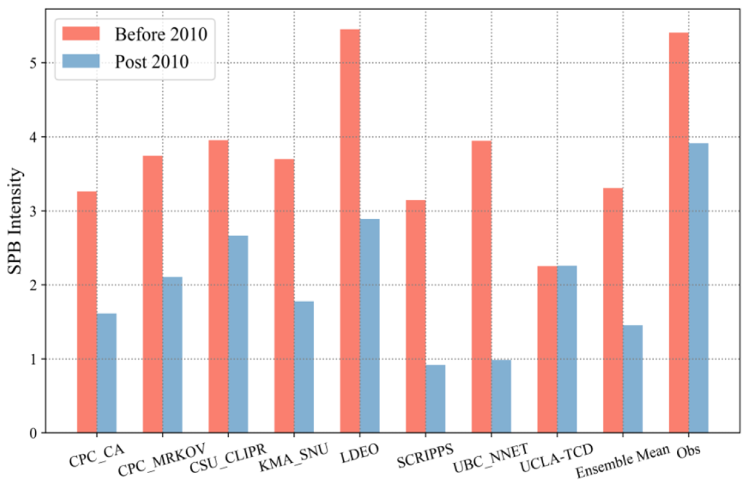
4. Decadal Variation of SPBS in IRI/CPC Multi-Model Prediction System

In the above sections, we defined an ENSO SPB index from the perspective of the zonal sea level pressure gradient, and found that SPBS exhibits significant decadal variations. Correspondingly, the atmosphere–ocean coupling state in the tropical Pacific also exhibits significant decadal variations. Corresponding to the period of weak SPBS, the tropical Pacific has an EP warming characteristic with stronger atmosphere–ocean coupling feedback, making ENSO signals more significant and difficult to be interrupted by other noises. During the period of strong SPBS, the tropical Pacific has a CP warming center with weak intensity. The weak atmosphere–ocean coupling feedback over the tropical Pacific weakens the ENSO signal, making it difficult to capture and predict. The rationality of the SPB index defined from the equatorial east–west Pacific sea level pressure gradient was well explained from the perspective of statistical analysis. However, regarding whether this decadal change really exists in ENSO prediction, we use multiple models from the operational ENSO prediction system of the US IRI/CPC to investigate the decadal variations of SPBS. Here we adopt an SPB intensity index defined in [35], which based on an ACF function to evaluate the SPBS in these models. The ACF (autocorrelation function) is a statistical tool employed to quantify the correlation of a given time series itself, which can be described as a function of initial months m and lag months τ [17,59], and written as r (m,τ). According to [35], ENSO SPBS can be defined from ACF as follows. First, for a calendar month m, we identify τ(m) as the specific lag of maximum ACF decline, which is calculated as the lag gradient in the time step of 1 month as

$$S_B(m)=\left\{{\displaystyle \frac{r\left[m,{\tau }_B\left(m\right)-1\right]-r\left[m,{\tau }_B\left(m\right)+1\right]}{2}}\right\}={max}_{\tau }\left[{\displaystyle \frac{r(m,\tau -1)-r(m,\tau +1)}{2}}\right]$$

(1)

where S_B (m) is the maximum gradient for every initial month. Second, the total intensity of the SPB is estimated as

$$S_{B_1}={\sum }_{m=1}^{12}{S}_B(m)$$

(2)

Figure 6 shows the SPB intensity calculated based on the prediction data of 10 models in IRI/CPC. Since all the prediction data we can obtain and test started after 2000, based on the above analysis, we divide the prediction data into two periods, 2001–2010 and 2011–2020, to study the decadal variation of SPBS in the models. It can be seen that except for UCLA-TCD, which has an approximate SPBS of around 2010, all other models exhibit stronger SPBS in the decade before 2010 than in the decade after 2010. This indicates that the decadal variation in the SPBS defined from the perspective of SLP gradient also exists in actual model predictions, which further validates the rationality of this SPB index.

5. Conclusions and Discussion

Based on the Bjerknes feedback theory and the decadal variation of the Walker circulation in the tropical Pacific, the seasonal variation in the observed zonal SLP gradient reveals a new perspective of SPB, which can reflect the stability and variability of atmosphere–ocean interactions during ENSO evolution. Our research shows that, in addition to the transition around 2000, a decadal variation of SPBS has been exhibited in the last 3 decades, synchronized with the decadal variation of standard deviation of the Nino3.4 index and the IPO index. The decadal variation of SPBS is closely related to the decadal variation of atmosphere–ocean coupling in the tropical Pacific. In the 1990s, the SSTa exhibited a typical EP ENSO pattern, with significant Bjerknes feedback enhancing ENSO signals, weakening noise interference, and making ENSO signals easier to capture and predict, resulting in weaker SPBS. In the 2000s, CP ENSO was prevalent, and weak atmosphere–ocean coupling and Bjerknes feedback made ENSO signals difficult to capture and predict, resulting in enhanced SPBS. In the 2010s, the SSTa was more like a combination of EP and CP type of ENSO, but the atmospheric response was more like the pattern of the 1990s, and the SPBS weakened again. The IRI/CPC multimodal prediction results also validate the rationality of the newly defined SPB index, which means that almost all models show stronger SPBS during the period of 2001–2010 compared to 2011–2020, consistent with statistical analysis.

ENSO itself is an anomalous phenomenon of atmosphere–ocean interaction, and ENSO SPB is regulated by the physical relationships governed by the strong atmosphere–ocean coupling over the tropical Pacific region [18,19,22,23]. Therefore, unlike many previous studies that define SPB from the perspective of SST [34,35], we attempt to define SPB from an atmospheric perspective and demonstrate its rationality in our study. Especially in the 2010s, SST exhibited a mixture of EP and CP type of ENSO, but the atmospheric response was more similar to that of the 1990s, and SPBS tended to weaken again, which well illustrates the advantages of defining SPB based on the zonal SLP gradient in the tropical Pacific.

Our study points out that the decadal variation of SPBS is strongly controlled by the dominant patterns of SST and Walker circulation over tropical Pacific, and associated with the background mean atmosphere–ocean states, which have also undergone a decadal variation over the past 3 decades. When explaining the mechanisms, ocean–atmosphere interaction was limited to SST, which does not mean that we exclude other potential factors, such as, for example, the decadal variation in the correlation between SST and thermocline depth [20,31,33]. As some researchers have pointed out, there is a strong coherence between the subsurface water temperatures and the atmospheric pressure drop at sea level induced by the ocean–atmosphere interaction in the central–eastern Pacific [60]. These may provide new perspectives for us to further analyze the mechanism of decadal variation in SPBS.

References

1. Zebiak, S.E.; Cane, M.A. A model El Niño-Southern Oscillation. Mon. Wea. Rev. 1987, 115, 2262–2278. [Google Scholar] [CrossRef]
2. Latif, M.; Anderson, D.; Barnett, T.; Cane, M.; Kleeman, R.; Leetmaa, A.; O’Brien, J.; Rosati, A.; Schneider, E. A review of the predictability and prediction of ENSO. J. Geophys. Res. 1998, 103, 14375–14393. [Google Scholar] [CrossRef]
3. Chen, D.; Cane, M.; Kaplan, A.; Zebiak, S.E.; Huang, D.J. Predictability of El Niño over the past 148 years. Nature 2004, 428, 733–736. [Google Scholar] [CrossRef]
4. Zheng, F.; Zhu, J.; Zhang, R.H.; Zhou, G. Improved ENSO forecasts byassimilating sea surface temperature observations into an intermediate coupled model. Adv. Atmos. Sci. 2006, 23, 615–624. [Google Scholar] [CrossRef]
5. Jin, E.K.; Kinter, J.L.; Wang, B.; Park, C.-K.; Kang, I.-S.; Kirtman, B.P.; Kug, J.-S.; Kumar, A.; Luo, J.-J.; Schemm, J.; et al. Current status of ENSO prediction skill in coupled ocean–atmosphere models. Clim. Dyn. 2008, 31, 647–664. [Google Scholar] [CrossRef]
6. Tippett, M.K.; Barnston, A.G. Skill of Multimodel ENSO Probability Forecasts. Mon. Wea. Rev. 2008, 136, 3933–3946. [Google Scholar] [CrossRef]
7. Luo, J.; Masson, S.; Behera, S.; Shingu, S.; Yamagata, T. Seasonal Climate Predictability in a Coupled OAGCM Using a Different Approach for Ensemble Forecasts. J. Clim. 2005, 18, 4474–4497. [Google Scholar] [CrossRef]
8. Barnston, A.G.; Tippett, M.K.; L’Heureux, M.L.; Li, S.; DeWitt, D.G. Skill of Real-Time Seasonal ENSO Model Predictions during 2002–11: Is Our Capability Increasing? Bull. Amer. Meteor. Soc. 2012, 93, ES48–ES50. [Google Scholar] [CrossRef]
9. Zheng, F.; Zhu, J. Improved ensemble-mean forecasting of ENSO events by a zero-mean stochastic error model of an intermediate coupled model. Clim. Dyn. 2016, 47, 3901–3915. [Google Scholar] [CrossRef]
10. Webster, P.J.; Yang, S. Monsoon and Enso: Selectively Interactive Systems. Q. J. R. Meteorol. Soc. 1992, 118, 877–926. [Google Scholar] [CrossRef]
11. Balmaseda, M.A.; Davey, M.K.; Anderson, D.L.T. Decadal and Seasonal Dependence of ENSO Prediction Skill. J. Clim. 1995, 8, 2705–2715. [Google Scholar] [CrossRef]
12. Zheng, F.; Zhu, J. Spring predictability barrier of ENSO events from the perspective of an ensemble prediction system. Glob. Planet. Chang. 2010, 72, 108–117. [Google Scholar] [CrossRef]
13. Duan, W.; Liu, X.; Zhu, K.; Mu, M. Exploring the initial errors that cause a significant “spring predictability barrier” for El Niño events. J. Geophys. Res. 2009, 114, C04022. [Google Scholar] [CrossRef]
14. Kirtman, B.P. The COLA Anomaly Coupled Model: Ensemble ENSO Prediction. Mon. Wea. Rev. 2003, 131, 2324–2341. [Google Scholar] [CrossRef]
15. Duan, W.; Hu, J. The initial errors that induce a significant “spring predictability barrier” for El Niño events and their implications for target observation: Results from an earth system model. Clim. Dyn. 2015, 46, 3599–3615. [Google Scholar] [CrossRef]
16. Duan, W.; Wei, C. The ‘spring predictability barrier’ for ENSO predictions and its possible mechanism: Results from a fully coupled model. Int. J. Climatol. 2012, 33, 1280–1292. [Google Scholar] [CrossRef]
17. Ren, H.-L.; Jin, F.-F.; Tian, B.; Scaife, A.A. Distinct persistence barriers in two types of ENSO. Geophys. Res. Lett. 2016, 43, 10973–10979. [Google Scholar] [CrossRef]
18. Jin, Y.; Liu, Z. A Theory of the Spring Persistence Barrier on ENSO. Part I: The Role of ENSO Period. J. Clim. 2021, 34, 2145–2155. [Google Scholar] [CrossRef]
19. Jin, Y.; Liu, Z.; Duan, W. The Different Relationships between the ENSO Spring Persistence Barrier and Predictability Barrier. J. Clim. 2022, 35, 6207–6218. [Google Scholar] [CrossRef]
20. McPhaden, M.J. Tropical Pacific Ocean heat content variations and ENSO persistence barriers. Geophys. Res. Lett. 2003, 30, 1480. [Google Scholar] [CrossRef]
21. Yu, J.Y.; Kao, H.-Y. Decadal changes of ENSO persistence barrier in SST and ocean heat content indices: 1958–2001. J. Geophys. Res. 2007, 112, D13106. [Google Scholar] [CrossRef]
22. Thompson, C.J.; Battisti, D.S. A Linear Stochastic Dynamical Model of ENSO. Part II: Analysis. J. Clim. 2001, 14, 445–466. [Google Scholar] [CrossRef]
23. Torrence, C.; Webster, P.J. The annual cycle of persistence in the El Niño/Southern Oscillation. Q. J. R. Meteorol. Soc. 1998, 124, 1985–2004. [Google Scholar] [CrossRef]
24. Hu, Z.; Kumar, A.; Ren, H.; Wang, H.; L’Heureux, M.; Jin, F. Weakened Interannual Variability in the Tropical Pacific Ocean since 2000. J. Clim. 2013, 26, 2601–2613. [Google Scholar] [CrossRef]
25. Kumar, A.; Hu, Z.Z. Interannual and interdecadal variability of ocean temperature along the equatorial Pacific in conjunction with ENSO. Clim. Dyn. 2014, 42, 1243–1258. [Google Scholar] [CrossRef]
26. Neske, S.; McGregor, S. Understanding the warm water volume precursor of ENSO events and its interdecadal variation. Geophys. Res. Lett. 2018, 45, 1577–1585. [Google Scholar] [CrossRef]
27. Hu, Z.; Kumar, A.; Huang, B.; Zhu, J.; L’Heureux, M.; McPhaden, M.J.; Yu, J. The Interdecadal Shift of ENSO Properties in 1999/2000: A Review. J. Clim. 2020, 33, 4441–4462. [Google Scholar] [CrossRef]
28. McPhaden, M.J.; Lee, T.; McClurg, D. El Niño and its relationship to changing background conditions in the tropical Pacific Ocean. Geophys. Res. Lett. 2011, 38, L15709. [Google Scholar] [CrossRef]
29. Kosaka, Y.; Xie, S.P. Recent global-warming hiatus tied to equatorial Pacific surface cooling. Nature 2013, 501, 403–407. [Google Scholar] [CrossRef]
30. Xiang, B.; Wang, B.; Li, T. A new paradigm for the predominance of standing Central Pacific Warming after the late 1990s. Clim. Dyn. 2013, 41, 327–340. [Google Scholar] [CrossRef]
31. Zhu, J.; Kumar, A.; Huang, B. The relationship between thermocline depth and SST anomalies in the eastern equatorial Pacific: Seasonality and decadal variations. Geophys. Res. Lett. 2015, 42, 4507–4515. [Google Scholar] [CrossRef]
32. Fang, X.H.; Mu, M. Both air-sea components are crucial for El Niño forecast from boreal spring. Sci. Rep. 2018, 8, 10501. [Google Scholar] [CrossRef]
33. Lübbecke, J.F.; McPhaden, M.J. Assessing the Twenty-First-Century Shift in ENSO Variability in Terms of the Bjerknes Stability Index. J. Clim. 2014, 27, 2577–2587. [Google Scholar] [CrossRef]
34. Fang, X.H.; Zheng, F.; Liu, Z.Y.; Zhu, J. Decadal modulation of ENSO spring persistence barrier by thermal damping processes in the observation. Geophys. Res. Lett. 2019, 46, 6892–6899. [Google Scholar] [CrossRef]
35. Liu, Z.; Jin, Y.; Rong, X. A theory for the seasonal predictability barrier: Threshold, timing, and intensity. J. Clim. 2019, 32, 423–443. [Google Scholar] [CrossRef]
36. Rayner, N.A.; Parker, D.E.; Horton, E.B.; Folland, C.K.; Alexander, L.V.; Rowell, D.P.; Kent, E.C.; Kaplan, A. Global analyses of sea surface temperature, sea ice, and night marine air temperature since the late nineteenth century. J. Geophys. Res. 2003, 108, 4407. [Google Scholar] [CrossRef]
37. Kalnay, E. Coauthors. The NCEP/NCAR 40-Year Reanalysis Project. Bull. Am. Meteor. Soc. 1996, 77, 437–472. [Google Scholar] [CrossRef]
38. Henley, B.J.; Gergis, J.; Karoly, D.J.; Power, S.; Kennedy, J.; Folland, C.K. A Tripole Index for the Interdecadal Pacific Oscillation. Clim. Dyn. 2015, 45, 3077–3090. [Google Scholar] [CrossRef]
39. Gelfand, A.E.; Dey, D.K. Bayesian Model Choice: Asymptotics and Exact Calculations. J. R. Stat. Soc. Ser. B 1994, 56, 501–514. [Google Scholar] [CrossRef]
40. Wang, B. The Vertical Structure and Development of the ENSO Anomaly Mode during 1979–1989. J. Atmos. Sci. 1992, 49, 698–712. [Google Scholar] [CrossRef]
41. An, S.; Wang, B. Mechanisms of Locking of the El Niño and La Niña Mature Phases to Boreal Winter. J. Clim. 2001, 14, 2164–2176. [Google Scholar] [CrossRef]
42. Yan, B.L. On the mechanism of the locking of the El Niño event onset phase to boreal spring. Adv. Atmos. Sci. 2005, 22, 741–750. [Google Scholar] [CrossRef]
43. Tian, B.; Ren, H.-L.; Jin, F.-F.; Stuecker, M.F. Diagnosing the representation and causes of the ENSO persistence barrier in CMIP5 simulations. Clim. Dyn. 2019, 53, 2147–2160. [Google Scholar] [CrossRef]
44. Clarke, A.J.; Gorder, S.V. The Connection between the Boreal Spring Southern Oscillation Persistence Barrier and Biennial Variability. J. Clim. 1999, 12, 610–620. [Google Scholar] [CrossRef]
45. Latif, M.; Barnett, T.P.; Cane, M.A.; Flügel, M.; Graham, N.E.; von Storch, H.; Xu, J.-S. A review of ENSO prediction studies. Clim. Dyn. 1994, 9, 167–179. [Google Scholar] [CrossRef]
46. Mu, M.; Xu, H.; Duan, W. A kind of initial errors related to “spring predictability barrier” for El Niño events in Zebiak-Cane model. Geophys. Res. Lett. 2007, 34, L03709. [Google Scholar] [CrossRef]
47. van Oldenborgh, G.J.; Balmaseda, M.A.; Ferranti, L.; Stockdale, T.N.; Anderson, D.L.T. Did the ECMWF Seasonal Forecast Model Outperform Statistical ENSO Forecast Models over the Last 15 Years? J. Clim. 2005, 18, 3240–3249. [Google Scholar] [CrossRef]
48. Webster, P.J. The annual cycle and the predictability of the tropical coupled ocean-atmosphere system. Meteorl. Atmos. Phys. 1995, 56, 33–55. [Google Scholar] [CrossRef]
49. Yu, J.-Y. Enhancement of ENSO’s persistence barrier by biennial variability in a coupled atmosphere-ocean general circulation model. Geophys. Res. Lett. 2005, 32, L13707. [Google Scholar] [CrossRef]
50. Wang, B.; Fu, X.H. Processes determining the rapid reestablishment of the equatorial Pacific cold tongue/ITCZ complex. J. Clim. 2001, 14, 2250–2265. [Google Scholar] [CrossRef]
51. Wang, B.; Wang, Y.Q. Dynamics of the itcz-equatorial cold tongue complex and causes of the latitudinal climate asymmetry. J. Clim. 1999, 12, 1830–1847. [Google Scholar] [CrossRef]
52. Philander, S.G.H. El Niño Southern Oscillation phenomena. Nature 1983, 302, 295–301. [Google Scholar] [CrossRef]
53. Battisti, D.S. Dynamics and thermodynamics of a warming event in a coupled tropical atmosphere–ocean model. J. Atmos. Sci. 1988, 45, 2889–2919. [Google Scholar] [CrossRef]
54. Tziperman, E.; Zebiak, S.E.; Cane, M.A. Mechanisms of seasonal–ENSO interaction. J. Atmos. Sci. 1997, 54, 61–71. [Google Scholar] [CrossRef]
55. Li, T. Phase transition of the El Niño–Southern Oscillation: A stationary SST mode. J. Atmos. Sci. 1997, 54, 2872–2887. [Google Scholar] [CrossRef]
56. Bjerknes, J. Atmospheric Teleconnections from the Equatorial Pacific. Mon. Weather. Rev. 1969, 97, 163–172. [Google Scholar] [CrossRef]
57. Okumura, Y.M.; Sun, T.; Wu, X. Asymmetric modulation of El Niño and La Niña and the linkage to tropical Pacific decadal variability. J. Clim. 2017, 30, 4705–4733. [Google Scholar] [CrossRef]
58. Lin, R.; Zheng, F.; Dong, X. ENSO frequency asymmetry and the Pacific decadal oscillation in observations and 19 CMIP5 models. Adv. Atmos. Sci. 2018, 35, 495–506. [Google Scholar] [CrossRef]
59. Jin, Y.; Lu, Z.; Liu, Z. Controls of spring persistence barrier strength in different ENSO regimes and implications for 21st century changes. Geophys. Res. Lett. 2020, 47, e2020GL088010. [Google Scholar] [CrossRef]
60. Jean-Louis, P. The Anticipation of the ENSO: What Resonantly Forced Baroclinic Waves Can Teach Us (Part II). J. Mar. Sci. Eng. 2018, 6, 63. [Google Scholar] [CrossRef]
Figure 2. MAM–mean (a) IPO index, (b) correlation coefficients between the SLP averaged over Indonesia and the EEP, and (c) standard deviation of the Niño3.4 index with 10-year moving windows for 1986–2022.
Jmse 12 01463 g002
Figure 3. Seasonal correlation coefficients between the SLP averaged over Indonesia and Equatorial Eastern Pacific for periods 1991–2000 (blue line), 2001–2010 (cyan line), and 2011–2020 (red line). Shading indicates the range of maximum and minimum correlation coefficients from the leave-one-out cross-validation for the period 2011–2020, and the dashed line shows that the correlation coefficients are significant at the 95% confidence level.
Jmse 12 01463 g003
Figure 4. Spatial patterns of the leading MEOF mode of atmospheric circulation fields (U-wind and omega; vertical) and the SST (85°E–60°W, 30°S–30°N; horizontal) during boreal spring. (a) The analysis period is 1991–2000, with the leading MEOF mode explaining 37.2% of the total variance. (b) The analysis period is 2001–2010, with the leading MEOF mode explaining 29.5% of the total variance. (c) The analysis period is 2011–2020, with the leading MEOF mode explaining 34.8% of the total variance.
Jmse 12 01463 g004
Figure 5. The east–west differences of the SST (red line) and SLP (black line) overlaid the IPO index during boreal spring of 1991–2021.
Jmse 12 01463 g005
Figure 6. The variation of spring predictability/persistence barrier (SPB) intensity between pre-2010 and post-2010 in IRI/CPC multi-models and observation.
Jmse 12 01463 g006
Disclaimer/Publisher’s Note: The statements, opinions and data contained in all publications are solely those of the individual author(s) and contributor(s) and not of MDPI and/or the editor(s). MDPI and/or the editor(s) disclaim responsibility for any injury to people or property resulting from any ideas, methods, instructions or products referred to in the content.