Abstract
Most existing model predictive control (MPC) methods overlook the network resource limitations of autonomous underwater vehicles (AUVs), limiting their applicability in real systems. This article addresses this gap by introducing an adaptive transmission, interval-based, and self-triggered model predictive control for AUVs operating under ocean disturbances. This approach enhances system stability while reducing resource consumption by optimizing MPC update frequencies and communication resource usage. Firstly, the method evaluates the discrepancy between system states at sampling instants and their optimal predictions. This significantly reduces the conservatism in the state-tracking errors caused by ocean disturbances compared to traditional approaches. Secondly, a self-triggering mechanism was employed, limiting information exchange to specified triggering instants to conserve communication resources more effectively. Lastly, by designing a robust terminal region and optimizing parameters, the recursive feasibility of the optimization problem is ensured, thereby maintaining the stability of the closed-loop system. The simulation results illustrate the efficacy of the controller.
1. Introduction
Autonomous underwater vehicles (AUVs) have emerged as crucial tools for exploring and exploiting ocean resources, capturing considerable interest from researchers globally [1]. Over the recent decades, AUVs have seen increased utilization across scientific, defense, and commercial sectors. Their primary uses encompass oceanographic mapping [2], gas extraction, and pipeline upkeep [3]. Additionally, they are used in maritime search, underwater object monitoring [4], and patrolling [5]. Precise control of AUVs is essential for these tasks [6,7] as underwater operations are susceptible to disturbances that impact positioning accuracy and control. Factors such as monsoons and sea waves can lead to significant errors and instability in trajectory tracking [8]. Therefore, designing effective anti-disturbance trajectory tracking controllers is crucial, drawing substantial attention from researchers worldwide.
Over the past few years, various control methodologies have emerged to tackle the challenge of tracking, including PID control [9], backstepping control (BSC) [10], and sliding-mode techniques [11]. However, engines have limited power, and mechanical components have maximum deflections or revolutions, imposing constraints on the vessel system. Ignoring these constraints during controller design may result in suboptimal performance or actuator damage during real-world implementation [12]. Model predictive control (MPC) is particularly suitable for managing constrained systems because of its explicit handling of constraints [13]. Since its initial formulation, MPC has seen extensive use in industrial applications [14,15]. For the tracking control of perturbed nonholonomic systems using MPC, prior research has utilized predicted state trajectories for current input [16]. Typically, only the first element of the control sequence generated by MPC is applied in each iteration [17]. Given the significant computational load involved in managing multiple constraints for nonholonomic systems [18], there is a growing interest in reducing the computational burden for the MPC-based tracking control of perturbed nonholonomic systems.
To address the limitations of traditional MPC, many researchers are working to enhance control sequence utilization and reduce computational load. This motivates the integration of the event-triggered strategy with MPC [19]. In event-triggered systems, the triggering time for transmission is determined based on specific conditions, often involving the error between predicted and actual states [20,21,22]. Another approach focuses on stabilizing the system by ensuring the optimal MPC value function decreases between consecutive time steps or triggering instances [23,24].
Since event-triggered MPC necessitates the continuous monitoring of states (whereas, in self-triggered MPC (STMPC), the subsequent triggered time is determined by the preceding one), the self-triggered strategy has garnered extensive research interest due to its lower demand for state information [25]. Refs. [26,27] concentrated on discrete-time systems, where the subsequent triggering moment and control inputs were jointly optimized to minimize a specified performance index. Given that numerous physical processes in AUVs operate continuously, STMPC has also been introduced for continuous-time systems. For example, the author in [28] proposed an STMPC algorithm with adaptive control sample selection for nonlinear systems. This control method determines the timing of control task execution and discretizes the optimal-control trajectory into multiple samples to reduce communication load. Meanwhile, the author in [29] integrated robust STMPC with a state-feedback control law. It is important that both the STMPC methodologies in [28,29] incorporate STMPC based on stability. A novel dual-STMPC strategy was proposed, significantly reducing the communication load, in [30]. However, there is still a need to solve optimization problems when the system state enters the terminal set, which incurs a certain computational burden compared to feedback control laws. They proposed a method to discretize the control input into multiple control samples, focusing solely on scenarios without disturbances.
Various studies have tackled the challenge of disturbances in self-triggered control systems. The trigger mechanism is designed using the decrement of the cost function [31,32]. However, both approaches result in a relatively conservative disturbance upper-bound-based feasibility proof. Additionally, when designing self-triggering mechanisms for systems with additional disturbances, the maximum value of disturbances over two triggering intervals is typically used [19,26,33]. This approach can result in considerable conservatism in state error, leading to an increased number of triggering instances. To tackle this challenge, this paper introduces a novel self-triggering mechanism. Readers interested in event-triggered or self-triggered MPC should consult Table 1 for additional information.

Table 1.
Representative works on event-triggered and self-triggered MPC.
Motivated by these insights, we devised an STMPC algorithm specifically for AUV systems that incorporate input constraints and bounded disturbances. The primary contributions of this paper are as follows:
- (1)
- To improve communication efficiency, this paper proposes a novel self-triggered mechanism. This mechanism determines sampling instants using the self-triggered approach and calculates the actual state prediction error based on the sampled states. This method reduces conservatism in state-error estimations. Compared to the traditional self-triggered mechanisms [26,31,33] that determine triggering times based on the maximum-error bound, this approach can lower the triggering frequency.
- (2)
- The proposed algorithm’s theoretical properties are detailed. A minimum inter-triggering interval is specified to prevent Zeno behavior, and adequate conditions are established to guarantee both algorithm feasibility and closed-loop stability. These theoretical results enhance the literature by offering feasibility guarantees that were not addressed in [28,34].
This paper will elaborate on the following sections. Section 2 establishes the AUV model and the design objectives. Section 3 presents the optimal-control problem along with the relevant constraints and designs a self-triggered mechanism, providing a proof for avoiding Zeno behavior. Section 4 analyzes the feasibility and stability of the optimization problem. Section 5 and Section 6 present simulations of the comparative outcomes and conclusions, respectively.
2. Problem Statement
2.1. AUV Model
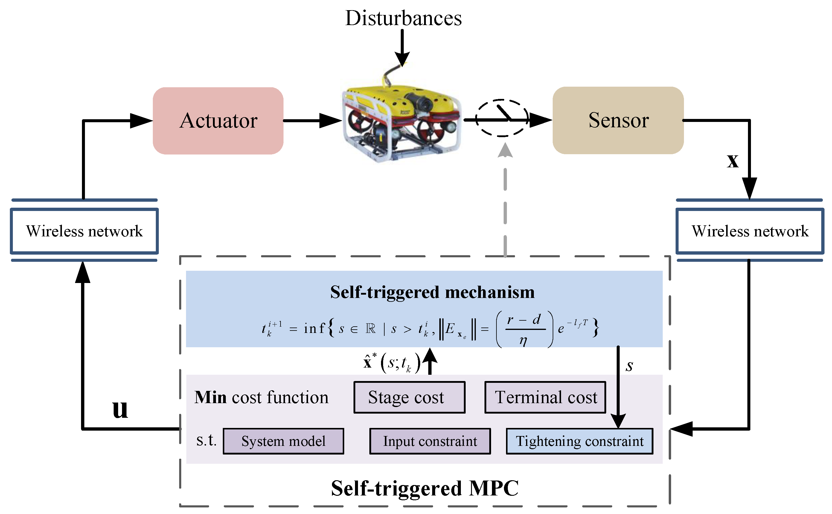
An AUV with the structure shown in Figure 1 was considered. This study focused on the horizontal movement of an AUV, with kinematic and dynamic equations characterized, as detailed in [35].
where depicts the position and heading; represents the vehicle’s velocity; ; signifies all the forces and moments exerted on the vehicle; and M, , and correspond to the inertia matrix, the Coriolis, the centripetal matrix, and the damping matrix, respectively.
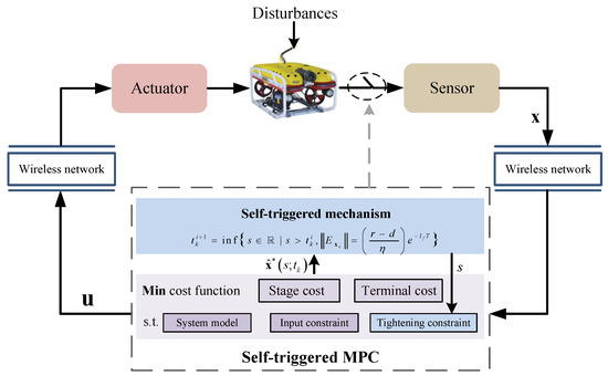
Figure 1.
A schematic representation of the STMPC system for an AUV.
The AUV model was based on combining (1) and (2):
where represents the practical system state, and represents practical control input. Additionally, and must comply with the following constraints: and , where and are compact convex sets with the origin included within their interior points. Note that represents external disturbances from wind, waves, and currents, which are bounded with an upper limit specified as .
The intended path for tracking is denoted by . We assumed that is three times differentiable. From the given trajectory , we can derive the desired AUV states , and .
It is simple to show that fulfills (1). Here, we assumed , and the control forces can be determined.
According to [36], the model for error dynamics can be derived as depicted below.
The state-error vector is defined as , and the control error vector is defined as . Hence, the nominal system for the error dynamics is presented as follows:
Assumption 1.
Given that the function : exhibits local Lipschitz continuity concerning , the associated Lipschitz constant was denoted as .
2.2. Design Objectives
Our goal was to effectively stabilize system (4) within a region encompassing the origin while conserving communication resources through less frequent optimization problem solving. To achieve this, we employed a dual-mode STMPC. If the state exited the terminal set, STMPC was used; otherwise, the controller switched to the terminal controller.
3. Main Results
3.1. Optimal-Control Problem
Before providing a detailed description of the optimal-control problem (OCP), we first defined the cost function. For the tracking-error system (4), the cost function was defined as follows:
where P, Q, and R represent the corresponding matrices that are positive definite, and T represents the prediction horizon. The OCP for tracking the AUV can thus be formulated as follows:
where is the optimal-control sequence, and the optimal state-error trajectory can be derived by applying to the nominal-error system (5).
Remark 1.
Note that the constraint set of state-error trajectories decreases with time. Compared to the conventional disturbance-free control strategy [30] that only imposes constraints on the terminal state , incorporating tightened constraints further enhances the robustness of the perturbed closed-loop system.
Assumption 2.
The positive definite matrices R and Q and a positive definite matrix P are such that (1) the set is an invariant set for AUV by setting with ; and (2) for a constant , there exists a local stabilizing control law that satisfies the following:
3.2. Self-Triggered Condition Design
Lemma 1.
For the AUV system, the strategy was designed depending on the difference between the actual and the nominal trajectory caused by unavoidable disturbances. The predictive errors were as follows:
The optimal-nominal trajectory at time was , while the actual system state resulting from applying the optimal-control sequence to System (3) was represented as , and denotes the actual state at the i-th sampling instant after the trigger time . , which represents the nominal-system state.
Proof.
Because disturbances were present, we obtained the actual state of the system at the sampling instant, thereby achieving a more accurate state error.
□
We devise a self-triggered approach to determine the subsequent sampling instant given that the OCP is addressed at time . The self-triggered mechanism design can be expressed as follows:
where .
Remark 2.
Observe that the condition for triggering in (14) is linked to the feasibility of the OCP when . Unlike the approach in [19,30], our derivation process for feasibility is distinct. Further details are provided in Section 4.1.
Remark 3.
The proposed self-triggered scheme offers significant advantages over existing methods. In traditional approaches such as those presented by [31,33], the upper limits of disturbances are used to estimate the actual predictive error in the state, leading to conservative outcomes and frequent triggering events. This conservatism arises from the impracticality of obtaining precise disturbances. To address this limitation, our method calculates the actual state of the AUV system and the error at each sampling instant. This approach significantly reduces the conservatism of state errors, thereby decreasing the frequency of triggering and enhancing overall system performance. Compared to event-triggered mechanisms [20,21,22], which rely on predefined conditions to initiate updates, our self-triggered approach offers greater adaptability and efficiency in handling varying system conditions and disturbances.
We defined the termination condition for sampling, which also dictates the subsequent triggering moment . The core concept is that if two consecutive sampling times and are sufficiently proximate, then . Since the number of control inputs depends on the prediction horizon, the number of samples is , so the subsequent triggering moment is .
In order to avoid the Zeno phenomenon in Algorithm 1, the minimum trigger interval is presented in Lemma 2.
| Algorithm 1 Self-triggered MPC algorithm |
| Input: Choose initial conditions T and initial state , |
| 1: if , then |
| 2: Utilize the locally stabilizing controller for the system outlined in System (4); |
| 3: else |
| 4: At time , determine the optimal-control inputs and the optimal state error |
| by solving (6). |
| 5: Based on the self-triggering condition (14), calculate the subsequent sampling instant |
| , and the combination of termination condition can be obtained . |
| 6: Implement the control for on the actual System (4). |
| 7: end if |
| 8: Update |
Lemma 2.
4. Recursive Feasibility and Stability Analysis
4.1. Recursive Feasibility Analysis
Assumption 3.
For , it is necessary to confirm that OCP possesses a resolution at . Consequently, the solution must satisfy both the control restriction and the final condition. A feasible control sequence at time is chosen as follows:
where represents the feasible state resulting from applying to the AUV system in (3). We then need to verify the feasible control inputs and states that satisfy the constraint condition.
Firstly, for , we need to prove that satisfies the constraint.
The last inequality utilizes the Gronwall–Bellman inequality and the triangle inequality. Due to the fact that the error accumulates over time, when , we plug in (19) and the self-triggered Mechanism (14), and we obtain the following:
Because satisfies (10), then the result is obtained.
Using Assumption 2, , we have
If we integrate the above formula from to , and substitute , we can finally obtain . Following Assumption 3, this leads to .
Secondly, for , we need to prove that satisfies Constraint (10). According to Formula (19), we can also obtain
Given condition Assumption 2, it follows that
The above procedure has shown that satisfies the terminal constraint, so using Assumption 3 can be obtained .
Thirdly, we demonstrate that can be achieved. The condition is met because of the feasibility of and Assumption 2 can guarantee that satisfies the input constraint.
4.2. Stability Analysis
With the incorporation of the self-triggered strategy in MPC, it is essential to examine the stability of the closed-loop system. Theorem presents the stability outcomes related to Algorithm 1.
Theorem 1.
For System (4), provided that the following conditions are met, we have
where represents the Lipschitz constant corresponding to the positive definite Matrix Q. If the initial tracking-error state starts in , we can infer that the tracking-error state will converge to the set in a finite time.
Proof.
Take a Lyapunov function as
From Inequality ; and Condition (19), for any , access is obtained as follows:
In order to more conveniently analyze, we can split into three parts and determine their respective upper bound values, such as where
For , evidently, we can obtain
As stated by [37], there exist constants such that . Consequently, can be determined as follows:
Based on (19), we can derive
Lastly, we can address the final segment. According to Assumption 1, differentiating it yields the following result.
By substituting Equation (36) into (30) and by utilizing the triangle inequality, we arrive at the following:
This ensures that the system state reaches in a finite time.
Then, when enters , System (4) will be governed by the feedback controller . When taking as the Lyapunov function [38], it indicates that is a robust positively invariant set. This concludes the proof. □
5. Simulation
In this section, simulation experiments are conducted on the classical AUV model parameters following [35], and MATLAB (R2020b) is used to validate the benefits of the STMPC controller. The anticipated trajectory is depicted below:
and the second case follows a figure-eight trajectory defined as
The prediction horizon ; Q and P are chosen as and ; and the control input is limited to . In our STMPC scheme, the system’s Lipschitz constant is calculated as being according to [39]. During simulation, the terminal region parameters were computed using the methodology outlined in reference [40].
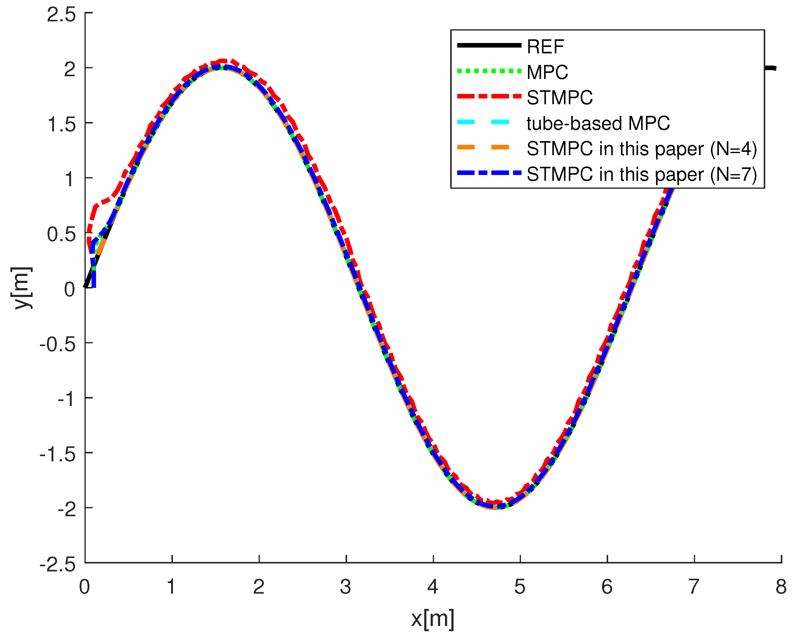
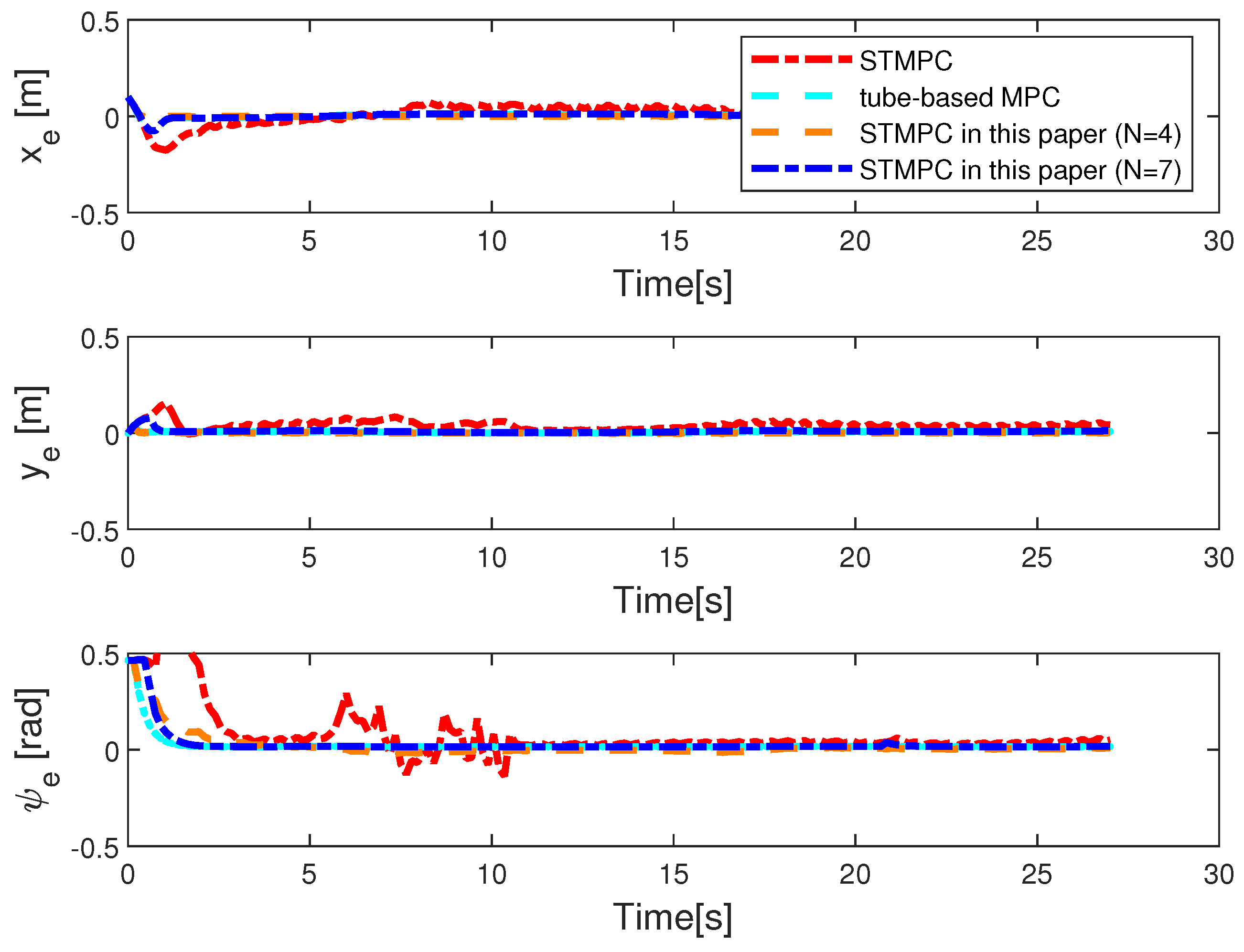
The trajectory-tracking outcomes for Case I are depicted in Figure 2 and Figure 3, with the initial system state set to . The black line represents the trajectories that need to be tracked, the green dashed line shows the tracking performance of the MPC in [41], the blue solid line illustrates the tracking performance of the rolling STMPC, and the magenta dash-dot line depicts the algorithm proposed in [31]. Double lines in turquoise indicate the tube-based MPC proposed in [36]. Based on the graphical illustration, it is evident that, under similar ocean disturbances, a tube-based MPC demonstrates better tracking performance. This is attributed to its capability of iteratively solving optimization problems within the same time horizon, thereby enabling the AUV to swiftly track the reference trajectory. This rationale holds because the optimal-control inputs derived from solving optimization problems offer advantages over suboptimal inputs. However, this approach imposes a significant computational burden. It is evident from the figure that our proposed STMPC scheme is viable. Figure 3 provide a comparison of the methods based on actual state trajectories. Figure 4 illustrates the tracking errors across STMPC algorithms. Specifically, under external disturbances, it was observed that each MPC controller steers the AUV toward convergence within a confined region.
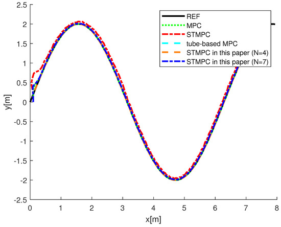
Figure 2.
Comparison of AUV system trajectory—Case I: MPC in [41], STMPC in [31], and tube-based MPC in [36].
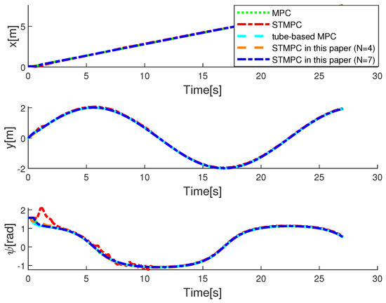
Figure 3.
State trajectories with disturbance—Case I: MPC in [41], STMPC in [31], and tube-based MPC in [36].
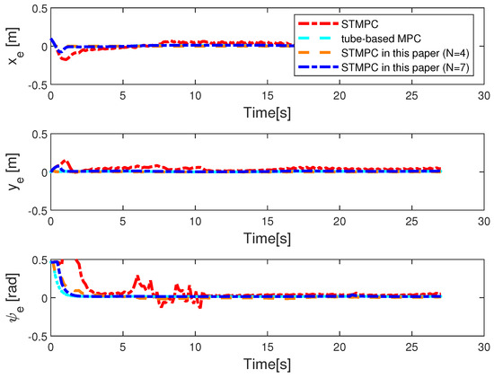
Figure 4.
Tracking deviations in the and dimensions using STMPC control strategies under the influence of disturbance. STMPC in [31]; tube-based MPC in [36].
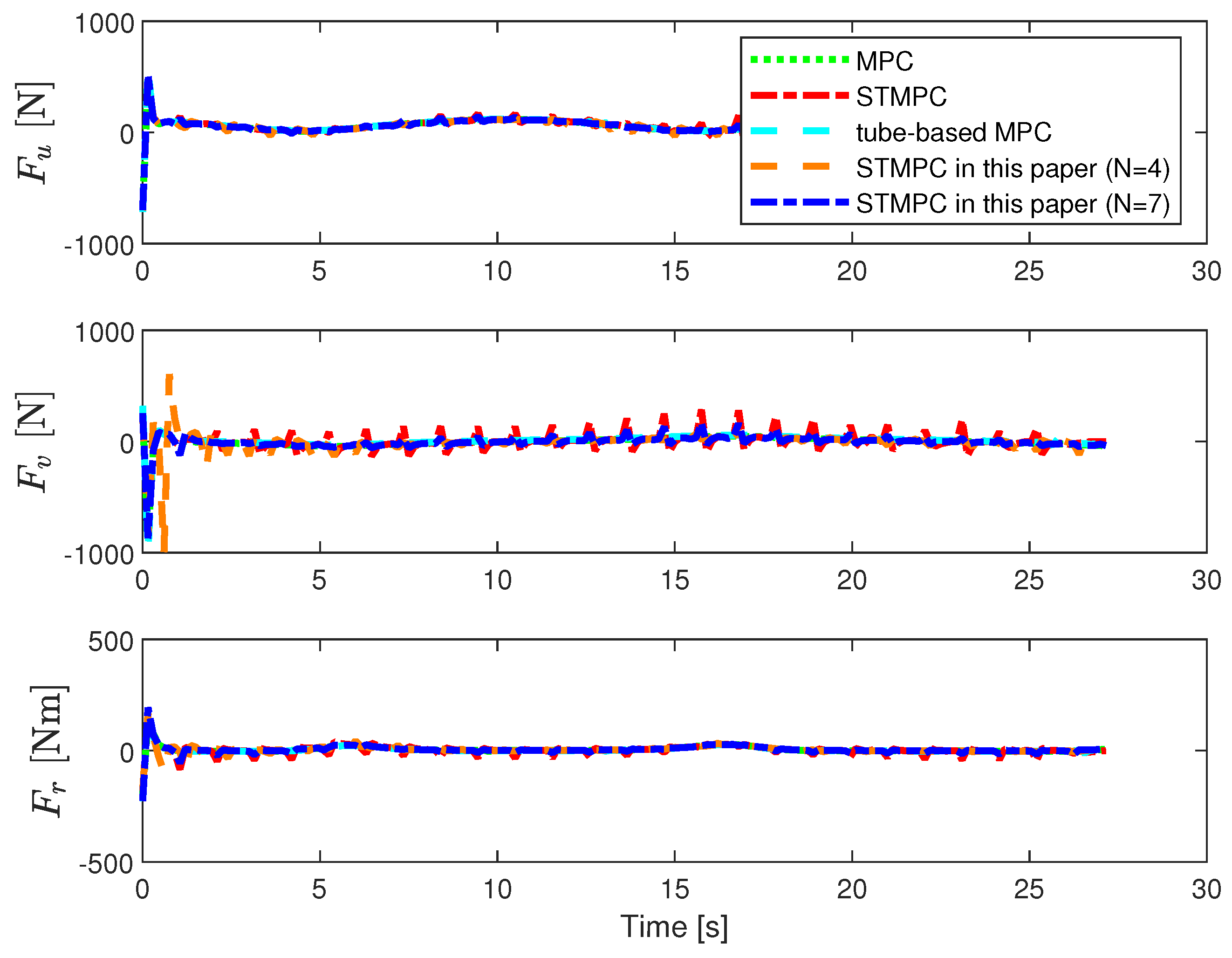
The control inputs for the AUV are depicted in Figure 5. We observed that, at the beginning of tracking, the STMPC controller maximized the utilization of onboard thrust to achieve the fastest possible convergence while respecting the physical constraints of the thrusters. Compared to the MPC in [41], our control inputs exhibit some oscillations, but the frequency of solving the OCP, as evidenced in Table 2, showed significant improvement. When compared to the STMPC in [31] under similar disturbance conditions, the control input oscillations were somewhat mitigated.
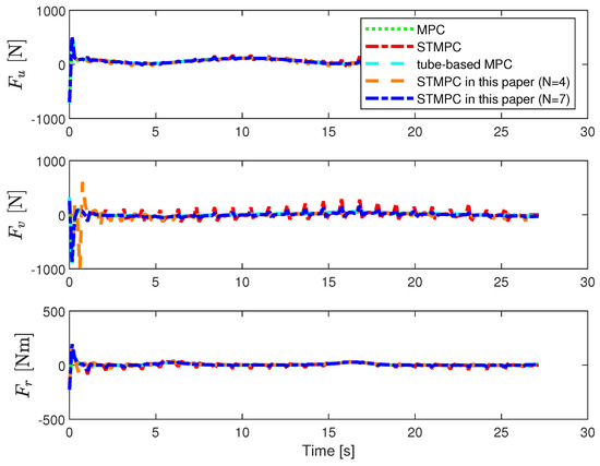
Figure 5.
Control input with disturbance—Case I: MPC in [41], STMPC in [31], and tube-based MPC in [36].
Table 2.
Comparison of the optimization problem’s total triggered times.
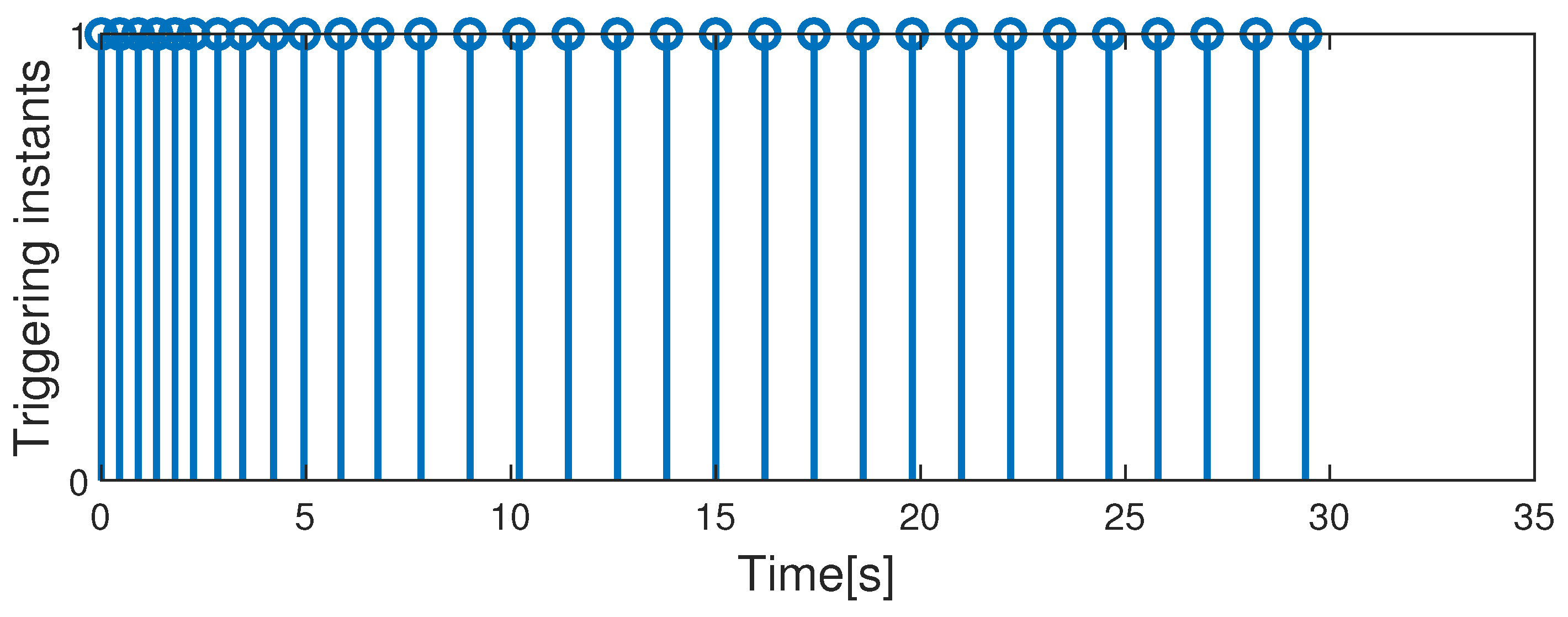
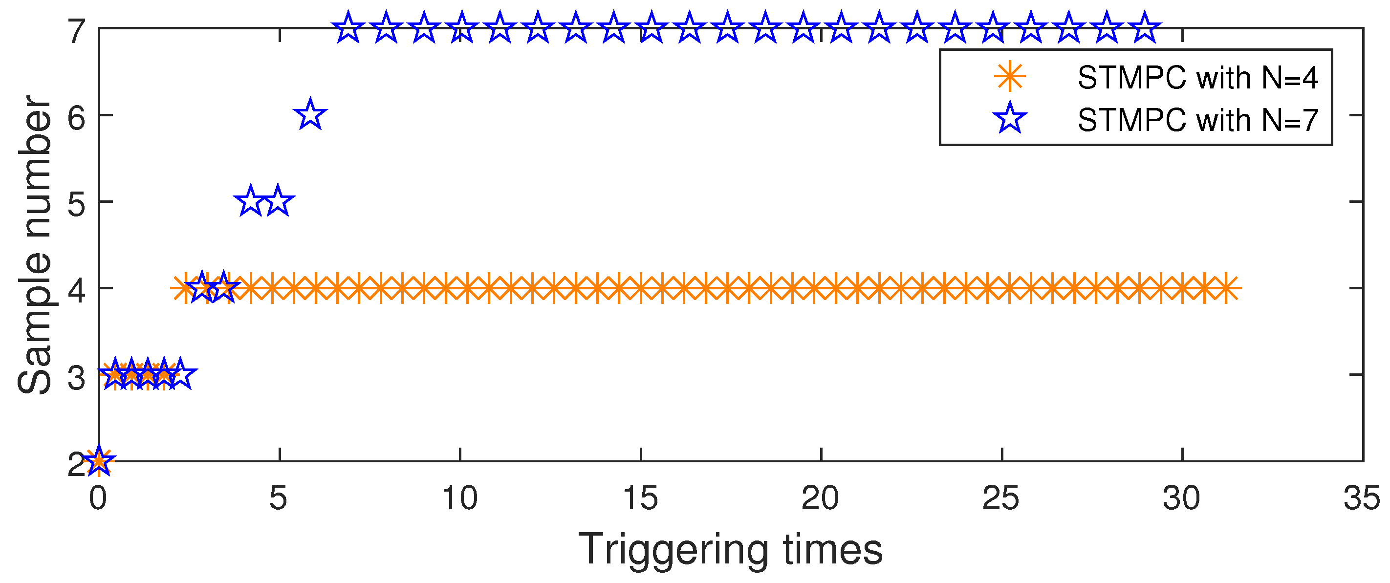
Additionally, as depicted in Figure 6, the count of the triggering events before the state trajectory entered the terminal set was finite using the proposed method, ensuring consistent performance. The AUV system also exhibited robustness against additive disturbances under the state-feedback controller. Figure 7 depicts obtaining a solution to an optimization problem at each triggering instant and applying the resulting control input sequence to the AUV system. In contrast to the tube-based MPC in [36], which utilizes only the first element of the control-input sequence per optimization solution, this method enhances the utilization of the control-input sequence. Consequently, the approach in this paper reduces the frequency of optimization problem solutions.

Figure 6.
Triggering times in the self-triggered mechanism.
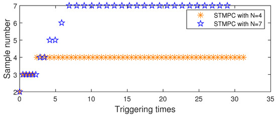
Figure 7.
Number of samples for each trigger instant at different prediction horizons.
To further illustrate the efficacy of the STMPC strategy, Table 2 provides a comparison of the computation solving times for OCP. The “Triggered times” column indicates the computation times of the OCP before steering the trajectory into the terminal set. It is evident that the STMPC strategy effectively reduces the number of optimization problem solutions and the time required during the tracking process, while ensuring a performance comparable to the MPC in [41]. Additionally, compared to the STMPC in [31], this approach further minimizes the number of solving instances and mitigates the conservatism in state errors under perturbations.
The simulation outcomes for Case II are illustrated in Figure 8 and Figure 9, with the initial system state set to . Comparable findings indicate that utilizing the proposed STMPC-based tracking control leads to a quicker convergence of the AUV to the desired trajectory, with consistently feasible control commands for the physical system.
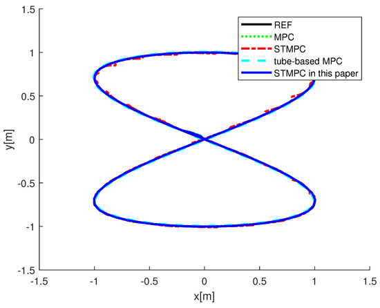
Figure 8.
Comparison of AUV system trajectory—Case II: MPC in [41], STMPC in [31], and tube-based MPC in [36].
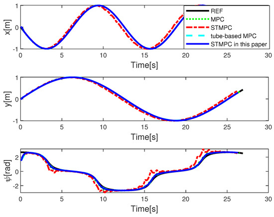
Figure 9.
State trajectories with disturbance—Case II: MPC in [41], STMPC in [31], and tube-based MPC in [36].
6. Conclusions
An adaptive transmission interval-based STMPC approach was proposed. This method designs a self-triggering mechanism by measuring the error between the actual tracking states at each sampling instant and their nominal counterparts, aiming to mitigate conservatism issues. By adopting this approach, we reduce the complexity of the MPC algorithm while preserving robust performance. Furthermore, significant reduction in communication overhead is achieved. This study establishes conditions for algorithmic feasibility and system stability. Lastly, the simulation conclusively demonstrates the theoretical results and effectiveness of the STMPC strategy.
Author Contributions
Conceptualization, L.H. and P.Z.; methodology, L.H. and P.Z.; software, P.Z.; validation, L.H. and P.Z.; formal analysis, P.Z.; investigation, P.Z.; resources, L.H.; data curation, R.W.; writing—original draft preparation, P.Z.; writing—review and editing, P.Z.; visualization, P.Z. and R.W.; supervision, R.W.; project administration, L.H.; funding acquisition, L.H. All authors have read and agreed to the published version of the manuscript.
Funding
This work is supported by the National Natural Science Foundation of China (Grant Nos. 52171292 and 51939001) and the Outstanding Young Talent Program of Dalian (Grant No. 2022RJ05).
Institutional Review Board Statement
Not applicable.
Informed Consent Statement
Not applicable.
Data Availability Statement
Data are contained within the article.
Conflicts of Interest
The authors declare no conflicts of interest.
References
- Xiang, X.; Lapierre, L.; Jouvencel, B. Smooth transition of AUV motion control: From fully-actuated to under-actuated configuration. Robot. Auton. Syst. 2015, 67, 14–22. [Google Scholar] [CrossRef]
- Zhang, F.; Marani, G.; Smith, R.N.; Choi, H.T. Future Trends in Marine Robotics. IEEE Robot. Autom. Mag. 2015, 22, 14–122. [Google Scholar] [CrossRef]
- Xiang, X.; Jouvencel, B.; Parodi, O. Coordinated Formation Control of Multiple Autonomous Underwater Vehicles for Pipeline Inspection. Int. J. Adv. Robot. Syst. 2010, 7, 75–84. [Google Scholar] [CrossRef]
- Ferri, G.; Munafò, A.; LePage, K.D. An Autonomous Underwater Vehicle Data-Driven Control Strategy for Target Tracking. IEEE J. Ocean. Eng. 2018, 43, 323–343. [Google Scholar] [CrossRef]
- Zhang, F.; Fratantoni, D.M.; Paley, D.A.; Lund, J.M.; Leonard, N.E. Control of coordinated patterns for ocean sampling. Int. J. Control 2007, 80, 1186–1199. [Google Scholar] [CrossRef]
- Refsnes, J.E.; Sorensen, A.J.; Pettersen, K.Y. Model-Based Output Feedback Control of Slender-Body Underactuated AUVs: Theory and Experiments. IEEE Trans. Control Syst. Technol. 2008, 16, 930–946. [Google Scholar] [CrossRef]
- Kim, J.; Joe, H.; Yu, S.c.; Lee, J.S.; Kim, M. Time-Delay Controller Design for Position Control of Autonomous Underwater Vehicle Under Disturbances. IEEE Trans. Ind. Electron. 2016, 63, 1052–1061. [Google Scholar] [CrossRef]
- Cui, R.; Zhang, X.; Cui, D. Adaptive sliding-mode attitude control for autonomous underwater vehicles with input nonlinearities. Ocean Eng. 2016, 123, 45–54. [Google Scholar] [CrossRef]
- Khodayari, M.H.; Balochian, S. Modeling and control of autonomous underwater vehicle (AUV) in heading and depth attitude via self-adaptive fuzzy PID controller. J. Mar. Sci. Technol. 2015, 20, 559–578. [Google Scholar] [CrossRef]
- Davila, J. Exact Tracking Using Backstepping Control Design and High-Order Sliding Modes. IEEE Trans. Autom. Control 2013, 58, 2077–2081. [Google Scholar] [CrossRef]
- Liao, Y.l.; Wan, L.; Zhuang, J.y. Backstepping dynamical sliding mode control method for the path following of the underactuated surface vessel. Procedia Eng. 2011, 15, 256–263. [Google Scholar] [CrossRef]
- Ding, W.; Zhang, L.; Zhang, G.; Wang, C.; Chai, Y.; Mao, Z. Research on 3D trajectory tracking of underactuated AUV under strong disturbance environment. Comput. Electr. Eng. 2023, 111, 108924. [Google Scholar] [CrossRef]
- Choi, W.Y.; Lee, S.H.; Chung, C.C. Horizonwise Model-Predictive Control With Application to Autonomous Driving Vehicle. IEEE Trans. Ind. Inform. 2022, 18, 6940–6949. [Google Scholar] [CrossRef]
- Rawlings, J.B.; Mayne, D.Q.; Diehl, M. Model Predictive Control: Theory, Computation, and Design; Nob Hill Publishing: Madison, WI, USA, 2017; Volume 2. [Google Scholar]
- Hao, L.Y.; Wu, Z.J.; Shen, C.; Cao, Y.; Wang, R.Z. Tube-Based Model Predictive Control for Constrained Unmanned Marine Vehicles With Thruster Faults. IEEE Trans. Ind. Inform. 2024, 20, 4606–4615. [Google Scholar] [CrossRef]
- Sun, Z.; Dai, L.; Liu, K.; Xia, Y.; Johansson, K.H. Robust MPC for tracking constrained unicycle robots with additive disturbances. Automatica 2018, 90, 172–184. [Google Scholar] [CrossRef]
- Wang, Q.; Duan, Z.; Lv, Y.; Wang, Q.; Chen, G. Distributed Model Predictive Control for Linear–Quadratic Performance and Consensus State Optimization of Multiagent Systems. IEEE Trans. Cybern. 2021, 51, 2905–2915. [Google Scholar] [CrossRef]
- Sun, Z.; Xia, Y.; Dai, L.; Liu, K.; Ma, D. Disturbance Rejection MPC for Tracking of Wheeled Mobile Robot. IEEE/ASME Trans. Mechatronics 2017, 22, 2576–2587. [Google Scholar] [CrossRef]
- Cao, Q.; Sun, Z.; Xia, Y.; Dai, L. Self-triggered MPC for trajectory tracking of unicycle-type robots with external disturbance. J. Frankl. Inst. 2019, 356, 5593–5610. [Google Scholar] [CrossRef]
- Li, H.; Shi, Y. Event-triggered robust model predictive control of continuous-time nonlinear systems. Automatica 2014, 50, 1507–1513. [Google Scholar] [CrossRef]
- Wang, M.; Sun, J.; Chen, J. Input-to-State Stability of Perturbed Nonlinear Systems With Event-Triggered Receding Horizon Control Scheme. IEEE Trans. Ind. Electron. 2019, 66, 6393–6403. [Google Scholar] [CrossRef]
- Wang, M.; Zhao, C.; Xia, J.; Sun, J. Periodic Event-Triggered Robust Distributed Model Predictive Control for Multiagent Systems With Input and Communication Delays. IEEE Trans. Ind. Inform. 2023, 19, 11216–11228. [Google Scholar] [CrossRef]
- Yoo, J.; Johansson, K.H. Event-Triggered Model Predictive Control With a Statistical Learning. IEEE Trans. Syst. Man Cybern. Syst. 2021, 51, 2571–2581. [Google Scholar] [CrossRef]
- Wang, M.; Cheng, P.; Zhang, Z.; Wang, M.; Chen, J. Periodic Event-Triggered MPC for Continuous-Time Nonlinear Systems With Bounded Disturbances. IEEE Trans. Autom. Control 2023, 68, 8036–8043. [Google Scholar] [CrossRef]
- Brunner, F.D.; Heemels, M.; Allgöwer, F. Robust self-triggered MPC for constrained linear systems: A tube-based approach. Automatica 2016, 72, 73–83. [Google Scholar] [CrossRef]
- Sun, Z.; Dai, L.; Liu, K.; Dimarogonas, D.V.; Xia, Y. Robust Self-Triggered MPC With Adaptive Prediction Horizon for Perturbed Nonlinear Systems. IEEE Trans. Autom. Control 2019, 64, 4780–4787. [Google Scholar] [CrossRef]
- Xie, H.; Dai, L.; Luo, Y.; Xia, Y. Robust MPC for disturbed nonlinear discrete-time systems via a composite self-triggered scheme. Automatica 2021, 127. [Google Scholar] [CrossRef]
- Hashimoto, K.; Adachi, S.; Dimarogonas, D.V. Self-Triggered Model Predictive Control for Nonlinear Input-Affine Dynamical Systems via Adaptive Control Samples Selection. IEEE Trans. Autom. Control 2017, 62, 177–189. [Google Scholar] [CrossRef]
- Luo, Y.; Xia, Y.; Sun, Z. Self-Triggered Model Predictive Control for Continue Linear Constrained System: Robustness and Stability. In Proceedings of the 2018 37th Chinese Control Conference (CCC), Wuhan, China, 25–27 July 2018; pp. 3612–3617. [Google Scholar]
- Cui, D.; Li, H. Dual Self-Triggered Model-Predictive Control for Nonlinear Cyber-Physical Systems. IEEE Trans. Syst. Man, Cybern. Syst. 2022, 52, 3442–3452. [Google Scholar] [CrossRef]
- Su, Y.; Wang, Q.; Sun, C. Self-triggered robust model predictive control for nonlinear systems with bounded disturbances. IET Control Theory Appl. 2019, 13, 1336–1343. [Google Scholar] [CrossRef]
- Yang, H.; Li, Q.; Zuo, Z.; Zhao, H. Self-triggered MPC for nonholonomic systems with multiple constraints by adaptive transmission intervals. Automatica 2021, 133, 109870. [Google Scholar] [CrossRef]
- Hashimoto, K.; Adachi, S.; Dimarogonas, D.V. Distributed aperiodic model predictive control for multi-agent systems. IET Control Theory Appl. 2015, 9, 10–20. [Google Scholar] [CrossRef]
- He, N.; Shi, D.; Chen, T. Self-triggered model predictive control for networked control systems based on first-order hold. Int. J. Robust Nonlinear Control 2018, 28, 1303–1318. [Google Scholar] [CrossRef]
- Shen, C.; Shi, Y.; Buckham, B. Integrated Path Planning and Tracking Control of an AUV: A Unified Receding Horizon Optimization Approach. IEEE/ASME Trans. Mechatronics 2017, 22, 1163–1173. [Google Scholar] [CrossRef]
- Hao, L.Y.; Wang, R.Z.; Shen, C.; Shi, Y. Trajectory Tracking Control of Autonomous Underwater Vehicles Using Improved Tube-Based Model Predictive Control Approach. IEEE Trans. Ind. Inform. 2024, 20, 5647–5657. [Google Scholar] [CrossRef]
- Paulavičius, R.; Žilinskas, J. Analysis of different norms and corresponding Lipschitz constants for global optimization. Technol. Econ. Dev. Econ. 2006, 12, 301–306. [Google Scholar] [CrossRef]
- He, N.; Ma, K.; Li, H.; Li, Y. Resilient Self-Triggered Model Predictive Control of Discrete-Time Nonlinear Cyberphysical Systems Against False Data Injection Attacks. IEEE Intell. Transp. Syst. Mag. 2023, 2–15. [Google Scholar] [CrossRef]
- Khalil, H.K. Nonlinear Systems; Prentice Hall: Upper Saddle River, NJ, USA, 2002. [Google Scholar]
- Eqtami, A.; Heshmati-alamdari, S.; Dimarogonas, D.V.; Kyriakopoulos, K.J. Self-triggered Model Predictive Control for nonholonomic systems. In Proceedings of the 2013 European Control Conference (ECC), Zurich, Switzerland, 17–19 July 2013; pp. 638–643. [Google Scholar]
- Yan, Z.; Yang, H.; Zhang, W.; Gong, Q.; Zhang, Y.; Zhao, L. Robust nonlinear model predictive control of a bionic underwater robot with external disturbances. Ocean Eng. 2022, 253, 111310. [Google Scholar] [CrossRef]


Disclaimer/Publisher’s Note: The statements, opinions and data contained in all publications are solely those of the individual author(s) and contributor(s) and not of MDPI and/or the editor(s). MDPI and/or the editor(s) disclaim responsibility for any injury to people or property resulting from any ideas, methods, instructions or products referred to in the content. |
© 2024 by the authors. Licensee MDPI, Basel, Switzerland. This article is an open access article distributed under the terms and conditions of the Creative Commons Attribution (CC BY) license (https://creativecommons.org/licenses/by/4.0/).