Numerical Study of Discharge Coefficients for Side-Damaged Compartments

Abstract

Accurately evaluating the buoyancy and stability of damaged ships, particularly the flow rate of the water inflow through damaged openings, is of great significance for ship rescue and emergency repair. A three-dimensional simplified model of inflow for a ship’s damaged side bulkheads is established using the shear stress transport k-epsilon and volume of fluid (VOF) models by STAR-CCM+. Moreover, the flow rates of water inflow through damaged openings with different shapes, characteristic sizes, and central depths are calculated. Furthermore, the corresponding discharge coefficients are obtained, and the relevant rules are summarized. It was found that the influence of water depth on the coefficient is minimal in these work conditions, but from the perspective of the damaged opening’s characteristic dimensions and shape, the variation in the coefficient is more pronounced. Overall, the triangular opening has a higher coefficient than the circular opening, which in turn is higher than that of the square-damaged opening, and the coefficient decreases as the size of the opening increases. Lastly, empirical formulas for two different methods are provided. The research provides a reference for the rescue repair and buoyancy stability assessment of damaged ships.

1. Introduction

Military ships are vulnerable to gunfire, torpedoes, anti-ship missiles, other ships, reefs, or sea structure impacts caused by hull damage; such damage can cause seawater to flow into cabins or liquid tanks to leak. If these leaks are not plugged in time, the ship’s maneuverability, self-sustaining, and strike efficiency may be affected, leading to capsizing and loss of personnel. Civilian ships also face the same risks, including reef impacts, collisions, trade blocking, unrestricted submarine warfare, and other forms of tactical warfare, which greatly influence the safety of civilian ship transportation.

Evaluating the technical status of the ship after damage, especially the loss of buoyancy, is an important part of the repair work in damage control. In 1942, the U.S. aircraft carrier USS Yorktown (CV-5) was hit by Japanese aircraft in the Battle of Midway, resulting in a large amount of seawater rushing into the compartments. The ship’s hull was damaged due to the commander’s misjudgment of the ship’s buoyancy and stability status. Moreover, the loss of control was missed; the CV-5 was attacked by a Japanese submarine and sank during the subsequent repair process. In 2018, the Norwegian frigate KNM Helge Ingstad (F-313) collided with a 62,000-ton tanker and ran aground, leading to serious injuries. The collision with a 62,000-ton tanker resulted in the ship running aground, causing a severe tear on the starboard side and a large amount of seawater rushing into the hold. The ship eventually capsized and sank. Thus, the importance of a timely and accurate assessment of the impact of breaching water ingress on a ship’s buoyancy and stability is self-evident. Hence, estimating the rate of breaching water ingress and calculating the time of the ship’s breaching water ingress are key issues in the assessment.

Theoretically, for viscous ideal fluid without considering the air compression effect, estimating the water inflow rate through the ship’s damaged opening is equivalent to the thin-walled small hole constant outflow problem. As shown in Figure 1, to maintain a constant water level, the cross-sectional area, S₁, of a thin-walled container is required. The container wall is at a distance from the reference surface height, z; the cross-sectional area of a small orifice is S₂, the vertical distance from the orifice to the water surface is H, atmospheric pressure is p, gravitational acceleration is g, the density of the liquid is ρ, the water level decrease rate in the container is v₁, and the orifice outflow rate is v. The law of conservation of mass and Bernoulli’s equation yield the following:

$$\left\{\begin{array}{c}{\displaystyle \frac{{v_1}^2}{2}}+{\displaystyle \frac{p}{2}}+g(z+H)={\displaystyle \frac{v^2}{2}}+{\displaystyle \frac{p}{\rho }}+gz\\ S_1{v}_1=S_{2}v\end{array}\right.$$

(1)

Equation (1) can be simplified as follows:

$$v=\sqrt{{\displaystyle \frac{2gH}{1-{(\frac{S_2}{S_1})}^2}}}$$

(2)

Equation (2) represents the liquid outflow rate from the small, thin-walled orifice. In particular, when $S_2\ll S_1$, Equation (2) can be simplified as follows:

$$v=\sqrt{2gH}$$

(3)

Equation (3) applies to seawater being poured into the compartments from the outboard side through the damaged opening but it does not apply to the diffusion of liquids or their discharge from the compartments to the outboard side.

This can lead to the theoretical formula used for calculating the flow rate through the opening, as follows:

$$Q=S_{2}v$$

(4)

where Q is the volume flow rate through the opening.

A large opening with thin walls can be conceptually divided into numerous small openings, as the flow rate varies at different points across the damaged surface. The flow rate through the damaged opening is obtained by integrating the flow velocity over the area of these small openings. Its average over the area is the average outflow velocity of the opening [1].

However, in reality, during the flow process, the gravitational potential energy of the liquid does not completely convert into kinetic energy. Some of the energy is dissipated due to the internal friction between liquid molecules, the friction between the liquid and the wall surfaces, and the contraction effect of the outflow at the breach, resulting in the actual flow rate being less than the flow rate calculated theoretically. As a result, the discharge coefficient, C_d (also known as the flow rate coefficient), is introduced to correct the flow rate through the opening defined via Equation (4):

$$Q_0=C_d·Q$$

(5)

where $Q_0$ is the actual volume flow rate through the breach.

In the boundary conditions, C_d is affected by the shape, size, location, and central depth of the opening. Moreover, there is no theoretical formula to calculate the value of C_d in the industry; it is usually empirically taken between 0.5 and 0.9 according to different situations. Furthermore, a half-empirical dimensionless pressure loss factor $k_{\mathrm{L}}$ is also commonly used to obtain a semi-empirical dimensionless pressure loss coefficient [2], as follows:

$$C_d={\displaystyle \frac{1}{\sqrt{1+k_L}}}$$

(6)

The method of obtaining the value of C_d must be investigated to obtain a more accurate breakwater inlet flow rate in the buoyancy stability assessment of damaged vessels, especially when using numerical methods, such as the quasi-static method [3]. In the past, the discharge coefficient was usually experimentally obtained. Vassalos [4] found that a coefficient discharge of 0.6 is a good approximation for the damaged opening. Ruponen [5,6,7] conducted a series of experimental studies on the damaged opening inlet of a box barge. The author found that the discharge coefficient fluctuated between 0.72 and 0.83 for damaged opening sizes ranging from 0.02 m × 0.02 m to 0.1 m × 0.1 m with different types of inlets. Moreover, the discharge coefficient decreases with an increase in the damaged opening size. Sterning [8] investigated the discharge coefficients of a ship’s cross-flooding duct through scale model experiments. The authors provided an essential dataset for the validation and further development of CFD approaches. Y. Li [9] conducted experimental studies on the discharge coefficient of petalled breaches and compared these results with the discharge coefficient of flat-edged damages. Wang [10] conducted a detailed experimental study of oil–water two-phase oil spill discharge coefficients for different damaged opening shapes, such as circular, square, elongated, and pentagonal. The design of the research program can be used as a reference for investigating the gas–liquid two-phase discharge coefficients.

With the vigorous development of CFD technology in recent years, parameters such as the mass flow rate of the damaged opening outflow can be directly obtained by numerical calculation, providing a new way to research discharge coefficients. Li [11] established a simplified two-dimensional single-chamber model using Fluent software and a k-epsilon turbulence model to simulate the discharge coefficients of ship breaches. The authors used the polynomial fitting method to provide the discharge coefficients and the relationship between the breaches and the aperture ratio, as follows:

$$C_d=0.641+0.00952{\displaystyle \frac{D}{h_c}}$$

(7)

where D is the damaged opening size and h_c is the distance from the center of the damaged opening to the water surface. However, the investigation did not consider the impact of factors such as the shape of the damaged opening on the discharge coefficient. Li [12,13] used Fluent software based on the box barge model to explore the discharge coefficients of specific breaches of double-hulled oil tankers. The author set up 16 conditions from different inlet and outlet water flow modes, different fluid level heights, shapes and sizes, fluid mediums, flooding situations of long openings, lateral water inlets with structures, commonly used damaged openings in the hull, double-hull bottom breakouts, and double-hull side breakouts, i.e., nine parameters were analyzed. The situations considered were comprehensive, but no detailed study was conducted on the individual angles. Hence, the results of each parameter were only provided for a single working condition.

Zhang [14] employed Fluent software to establish a simplified model of half-cylindrical compartments. The author employed a simplified model of a semi-cylindrical cabin to simulate the bottom-damaged opening of the ship, obtaining a discharge coefficient of approximately 0.65. Moreover, the author also noted that the irregular edge reduces the value of the inlet discharge coefficient. Furthermore, increasing the size of the damaged opening increases the inlet discharge coefficient slightly; however, it is set up with fewer working conditions (eight groups). The characteristic sizes of the damaged opening are small (0.0197–0.0394 m), and the depths of the water are also small (0.3 m and 0.5 m). Xue [15] used the shear stress transport k-epsilon and volume of fluid (VOF) models to analyze the attitude and resistance of a side-damaged frigate DTMB-5415. Wei [16,17] used the slip mesh method to develop numerical calculations for the discharge coefficients of square and circular flow holes of the SUBOFF submarine model with different drafts and sizes. However, the area of the flow holes was too small (0.004–0.016 m²). In addition, the study’s results could hardly be applied to the problem of valuing the discharge coefficients of the breaches of the damaged ship. Hu [18] used the VOF method to simulate the discharge coefficient of the circular drainage hole of the closed cavity and summarized the relevant laws. However, his research mainly focused on the drainage holes of aircraft, which are on the millimeter scale in diameter. Since the cabin damage and water ingress are not closed-cavity drainage models, his conclusions do not apply to ship damage issues, but his research methods can be used for reference.

There have been extensive investigations on discharge coefficients, but a universal empirical formula applicable to the ship breakout water intake problem has not yet been developed. In this paper, the discharge coefficient of the simplified model of the ship’s side-damaged opening is calculated using the RANS method and VOF model, using commercial fluid numerical computation software STAR-CCM+ (version 2402). Moreover, the relationship between the water intake discharge coefficient and parameters, such as the shape of the damaged opening, the area, the characteristic size, and the depth of the center, is provided based on the idea of control variables. This ‘law’ can provide a certain reference basis for the assessment of the buoyancy state of a breached ship and for making decisions on damage control. Moreover, the research results can provide a reference basis for assessing the buoyancy and stability of damaged ships and for guiding decisions on damage management.

2. Computational Principles and Numerical Modeling

2.1. Principle of Discharge Coefficient Calculation

A CFD simulation of the damaged ship’s damaged opening outflow process was conducted. The damaged opening mass flow rate was monitored and employed to calculate the average velocity of the damaged opening outflow. The results were compared with the theoretical velocity (hereinafter referred to as the average method) or with the theoretical velocity of the theoretical mass flow rate, which is obtained by dividing the area of the theoretical mass flow rate by the mass flow rate of the numerical calculation (hereinafter referred to as the integral method). Hence, the discharge coefficient is obtained.

(1)

Averaging:

The mass flow rate of the damaged opening, obtained by numerical calculation, is M₀ (unit: kg/s), the cross-sectional area of the damaged opening is S₂ (unit: m²), and the density of the liquid is ρ (unit: kg/m³). The average flow rate of the damaged opening outflow v₀ (unit: m/s) is as follows:

$$v_0={\displaystyle \frac{M_0}{\rho S_2}}$$

(8)

The discharge coefficient can be obtained by considering the theoretical flow rate at the center of the damaged opening as the average theoretical flow rate, v, as follows:

$$C_d={\displaystyle \frac{v_0}{v}}$$

(9)

(2)

Integral method:

The theoretical mass flow rate M (unit: kg/s) is obtained by dividing the area of the theoretical flow rate, v, with the liquid density, ρ, in the damaged opening cross-section, as follows:

$$M={\displaystyle {\int }_{S_2}\rho vds}$$

(10)

The discharge coefficient is as follows:

$$C_d={\displaystyle \frac{M_0}{M}}$$

(11)

The discharge coefficients obtained from the two methods are consistent [19].

2.2. Control Equations

The three-dimensional incompressible viscous fluid transient equations of motion are used as the theoretical basis. Moreover, the fluid density and the viscosity coefficient are assumed to be constants.

The mass conservation equation (the continuity equation) can be expressed as follows:

$${\displaystyle \frac{\partial u}{\partial x}}+{\displaystyle \frac{\partial v}{\partial y}}+{\displaystyle \frac{\partial w}{\partial z}}=0$$

(12)

where u, v, and w are the velocity components of the velocity vector, v, along the x, y, and z axes, respectively.

The equation of conservation of momentum (equation of motion) can be expressed as follows:

$$\rho {\displaystyle \frac{dv}{dt}}=\rho F-gradp+\mu {\nabla }^{2}v$$

(13)

where f is the mass force, p is the pressure, and μ is the hydrodynamic viscosity.

2.3. Turbulence Modeling

Navier–Stokes (N-S) equations can be expressed as follows:

$$\left\{\begin{array}{c}{\displaystyle \frac{\partial (\rho u)}{\partial t}}+\nabla (\rho uV)=-{\displaystyle \frac{\partial p}{\partial x}}+{\displaystyle \frac{\partial {\tau }_{xx}}{\partial x}}+{\displaystyle \frac{\partial {\tau }_{yx}}{\partial y}}+{\displaystyle \frac{\partial {\tau }_{zx}}{\partial z}}+\rho f_x\\ {\displaystyle \frac{\partial (\rho u)}{\partial t}}+\nabla (\rho vV)=-{\displaystyle \frac{\partial p}{\partial y}}+{\displaystyle \frac{\partial {\tau }_{xy}}{\partial x}}+{\displaystyle \frac{\partial {\tau }_{yy}}{\partial y}}+{\displaystyle \frac{\partial {\tau }_{zy}}{\partial z}}+\rho f_y\\ {\displaystyle \frac{\partial (\rho u)}{\partial t}}+\nabla (\rho wV)=-{\displaystyle \frac{\partial p}{\partial z}}+{\displaystyle \frac{\partial {\tau }_{xz}}{\partial x}}+{\displaystyle \frac{\partial {\tau }_{yz}}{\partial y}}+{\displaystyle \frac{\partial {\tau }_{zz}}{\partial z}}+\rho f_z\end{array}\right.$$

(14)

where p is the pressure, ${\tau }_{xx},\dots \dots ,{\tau }_{zz}$ is the component of the viscous stress τ, and $f_x,f_y,f_z$ denotes the force per unit mass in the x, y, and z directions, respectively.

Since it is very difficult to solve the N-S equations directly, the Reynolds-averaged Navier–Stokes (RANS) equations are used to perform simplified solution calculations by averaging the unsteady flow control equations over time and only considering large-scale time-averaged flows.

k-epsilon turbulence modeling equations can be expressed as follows:

$$\left\{\begin{array}{c}{\displaystyle \frac{\partial \left(\rho k\right)}{\partial t}}+{\displaystyle \frac{\partial \left(\rho k{u}_i\right)}{\partial x_i}}={\displaystyle \frac{\partial }{\partial x_j}}\left[(\mu +{\displaystyle \frac{{\mu }_i}{{\sigma }_k}}){\displaystyle \frac{\partial k}{\partial x_j}}\right]+G_k+G_b-\rho \epsilon -Y_m+S_k\\ {\displaystyle \frac{\partial \left(\rho \epsilon \right)}{\partial t}}+{\displaystyle \frac{\partial \left(\rho \epsilon u_i\right)}{\partial x_i}}={\displaystyle \frac{\partial }{\partial x_j}}\left[(\mu +{\displaystyle \frac{{\mu }_i}{{\sigma }_{\epsilon }}}){\displaystyle \frac{\partial \epsilon }{\partial x_j}}\right]+C_{1\epsilon }{\displaystyle \frac{\epsilon }{k}}(G_k+C_{3\epsilon }{G}_b)-C_{2\epsilon }\rho {\displaystyle \frac{{\epsilon }^2}{k}}+S_{\epsilon }\end{array}\right.$$

(15)

where $G_k,G_b$ are the turbulent kinetic energy terms generated by the velocity gradient and buoyancy, respectively. Parameters $i,j=\mathrm{1,2},3$ denote the x, y, and z directions, respectively, $Y_m$ is the pulsation expansion term, $C_{1ϵ},C_{2\epsilon },C_{3\epsilon }$ is an empirical constant, ${\sigma }_k,{\sigma }_{ϵ}$ is the Prandtl number corresponding to the turbulent kinetic energy k and dissipation rate ε, and $S_k,S_{\epsilon }$ is the user-defined source term.

2.4. Free Level Treatment

The Eulerian multiphase flow-volume of fluid (VOF) domain model can be expressed as follows:

$$\left\{\begin{array}{c}{\displaystyle \frac{\partial }{\partial t}}r\rho v+\nabla r\rho v=0\\ {\displaystyle \frac{\partial }{\partial t}}(1-r){\rho }_{a}v+\nabla (1-r){\rho }_{a}v=0\end{array}\right.$$

(16)

where r is the water volume fraction and ${\rho }_a$ is the density of air. The VOF method can model stratified multiphase fluids with large-scale interfaces, where the interphase interface is determined by solving the volume fractions of water and air in each control cell.

The free surface is defined by the isosurface, where the water volume fraction is 0.5 (i.e., equal to the volume fraction of air).

3. Simplified Modeling and Design of Working Conditions

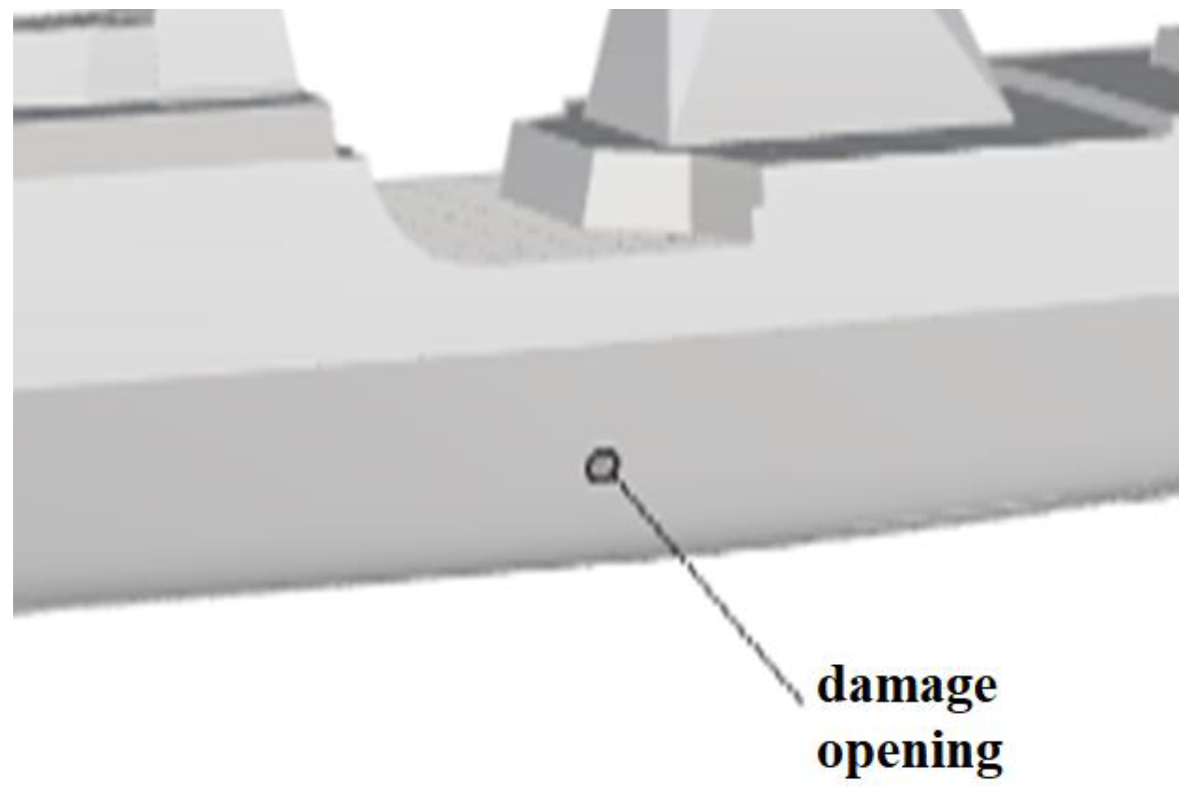
3.1. Basic Model

The main focus of this paper is the breakthrough law governing the water inlet discharge coefficient when the ship-side shell plate is damaged. Therefore, the model should meet the following requirements.

• The breakthrough surface is vertical or nearly vertical to the horizontal plane, in line with the typical characteristics of the ship-side shell plate arrangement.
• The breakthrough is completely located below the water line, enabling the seawater to pass through the entire breakthrough into the cabin.
• The size of the damaged opening should not be too small or too large because the unsuitable damaged opening size makes the study lose its practical significance.
• The damaged opening chamber must be open and spacious to avoid the impact of the jet stream on the bulkheads or other structures on the calculation.

A typical local model of a damaged ship is shown in Figure 2.

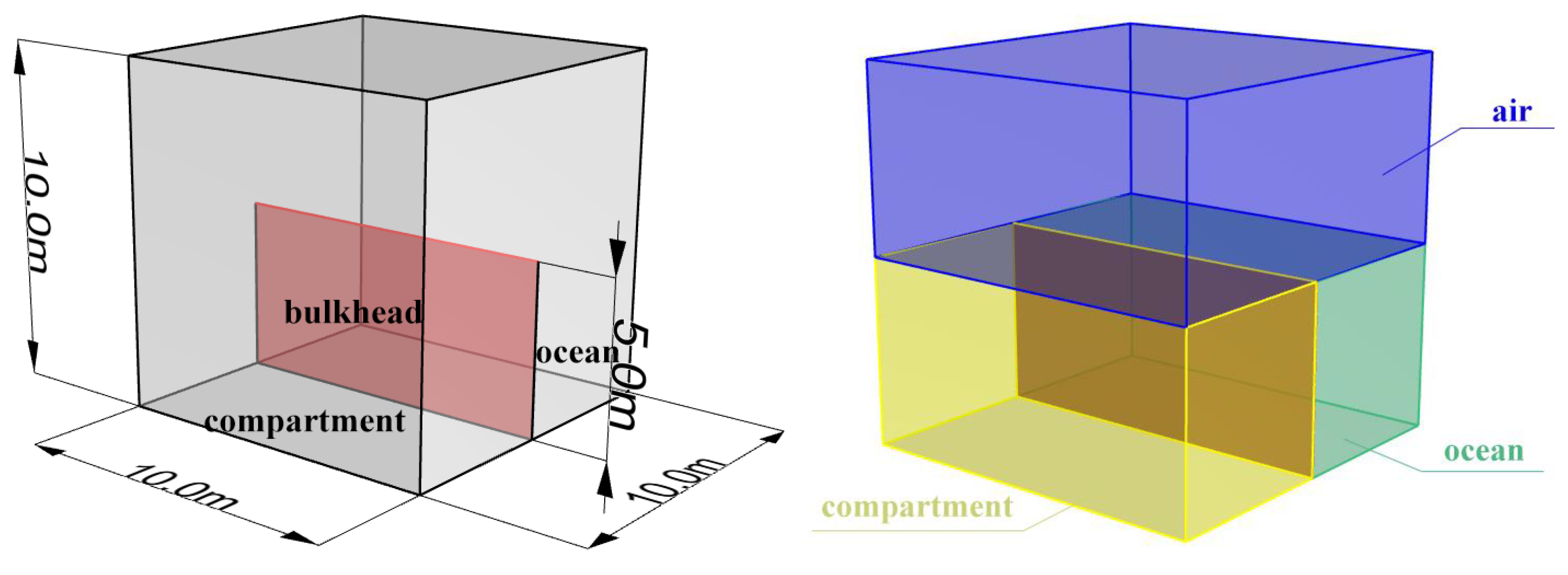
3.2. Simplified Model

Since most of the hull is irrelevant to the calculation, a simplified model can be intercepted from the relevant part of the damaged ship model to improve the speed and efficiency of modeling and calculation.

The simplified computational model is shown in Figure 3. The hexahedral computational domain is 10 m long, with a built-in bulkhead (red part) 10 mm thick to simulate the ship-side shell plate. The computational domain is divided into two parts. The first part is filled with seawater to simulate the marine environment, while the other represents the empty compartment. The upper part connects to the atmosphere to avoid the uneven air pressure affecting the computation. The middle part of the bulkhead is equipped with openings of various shapes, depths, and sizes to simulate various battle damage scenarios.

3.3. Design of Working Conditions

We assumed that the ship was hit with an anti-ship weapon below the waterline on the side shell plate, resulting in a large amount of seawater rushing into the cabin. Thus, a total of 150 scenarios were designed based on common opening shapes, positions, and characteristic dimensions of damaged ships to investigate the relationship between the shape, depth, and size of the damaged opening and the discharge coefficient. Three different shapes of openings were designed: circular, square, and triangular. Five different central depths of the damaged openings were set, as follows: 1 m, 1.5 m, 2 m, 2.5 m, and 3 m. Ten different scenarios were set according to the parameters of the typical main guns of warships, torpedoes, and anti-ship missiles (

Table 1. Parameters of typical anti-ship weapons.

Main Guns		Torpedoes		Anti-Ship Missiles
Ship Classification	Caliber (mm)	Type	Caliber (mm)	Type	Caliber (mm)
Arleigh Burke	127	MK48	533	AGM-109	520
Ticonderoga	127	Sailfish	533	Hsiung Feng III	460
Sejong Daewang	127	Varunastra	533	AGM-84	340
Chilung	127	MK46	324	Type 12	350
Murasame	76	MU-90	324	P-J10	670

) for the characteristic dimensions of the damage openings, as follows: 0.1 m, 0.2 m, 0.3 m, 0.4 m, 0.5 m, 0.6 m, 0.7 m, 0.8 m, 0.9 m, and 1 m The maximum value of the ratio of the characteristic size of the damaged opening to the thickness of the bulkhead was 0.01/0.05 = 0.2. Since this value is less than 2, the damaged opening can be considered to belong to the category of thin damaged openings. All working conditions are shown in

Table 2. All working conditions.

Type	Size (m)	Number in Different Depth of Damaged Opening Center
		1.0 m	1.5 m	2.0 m	2.5 m	3.0 m
Circular	0.1	No. 1	No. 11	No. 21	No. 31	No. 41
Circular	0.2	No. 2	No. 12	No. 22	No. 32	No. 42
Circular	0.3	No. 3	No. 13	No. 23	No. 33	No. 43
Circular	……	……	……	……	……	……
Circular	1.0	No. 10	No. 20	No. 30	No. 40	No. 50
Square	0.1	No. 51	No. 61	No. 71	No. 81	No. 91
Square	0.2	No. 52	No. 62	No. 72	No. 82	No. 92
Square	0.3	No. 53	No. 63	No. 73	No. 83	No. 93
Square	……	……	……	……	……	……
Square	1.0	No. 60	No. 70	No. 80	No. 90	No. 100
Triangular	0.1	No. 101	No. 111	No. 121	No. 131	No. 141
Triangular	0.2	No. 102	No. 112	No. 122	No. 132	No. 142
Triangular	0.3	No. 103	No. 113	No. 123	No. 133	No. 143
Triangular	……	……	……	……	……	……
Triangular	1.0	No. 110	No. 120	No. 130	No. 140	No. 150

.

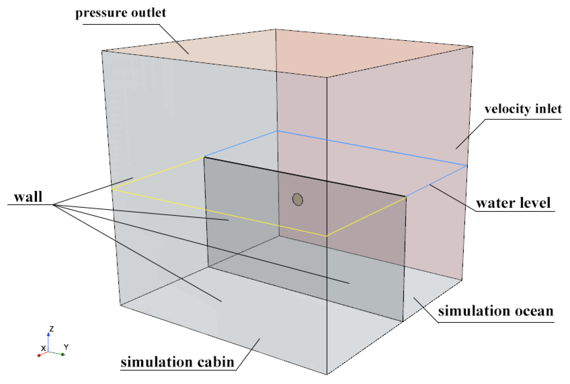
4. Numerical Simulation Points

The physical continuum model is multiphase and incorporates the volume of fluid (VOF) domain, k-epsilon turbulence, implicit unsteady state, VOF wave, and gravity. Two new phases were created in the multiphase-Eulerian phase, denoted as water and air. A liquid constant density was chosen to model the water, and a gaseous ideal gas was chosen to model the air. A new hydrostatic VOF wave was created in the VOF wave, and the point on the water level was made to be in the plane at the top of the divider.

The solver time step is set at 0.01 s, with the stopping criterion being the maximum physical time of 1 s, i.e., the program calculates in intervals of 0.01 s until it stops at 1 s.

Boundary Condition Settings and Post-Processing

The top of the computational domain was set as a pressure outlet to ensure that the pressure in the computational domain remained stable. The back wall of the pool represents the velocity inlet (the light red portion in Figure 4), while the remainder of the surface represents the wall.

A new mass flow monitor report on the damaged opening and a mass flow (kg/s) − time (s) plot were created based on the corresponding monitor. Moreover, a longitudinal profile was created through the damaged opening in the derived parts, and a scalar scene was created. Lastly, the longitudinal profile displays a color mapping plot of the water volume fraction.

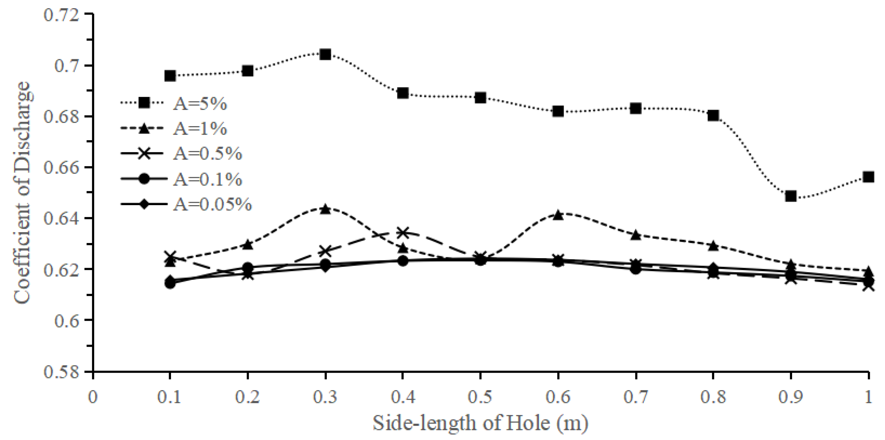
5. Mesh Division and Irrelevance Test

The mesh delineation quality greatly impacts CFD calculations. In general, the finer the mesh, the more accurate the calculation. However, the calculation time decreases with coarser mesh, but at the expense of accuracy.

The cut body mesh cell generator was selected for this calculation model. The base size of 1.0 m, target surface size of 100%, minimum surface size of 10%, very slow volume growth rate, and maximum mesh cell size of 100% were set. In addition to mesh encryption for the divider, the jet region, and the free liquid surface, the divider surface was encrypted with a target surface size of 10% (0.1 m). The minimum surface size was 1% (0.01 m), the surface of the inner wall of the damaged opening was encrypted with a target size of 1% (0.01 m), the jet region was encrypted with a customized isotropic encryption of 10% (0.1 m), and the free liquid surface region was encrypted with a customized Z-direction encryption of 10% (0.1 m).

The mesh of the damaged opening area, particularly the mesh of the opening wall, was a key factor affecting the flow rate of the calculation results. The encryption parameters of the mesh surface and the mesh-independence verification were carried out for the opening wall of the damaged opening. The smaller the characteristic size of the damaged opening, the more the flow phenomenon was affected by the friction of the opening wall. Therefore, the smaller the damaged opening, the smaller the encryption size of the opening wall mesh. Encryption parameter A is defined as follows:

$$\mathrm{A}={\displaystyle \frac{\mathrm{Absolute} \mathrm{valute} \mathrm{of} \mathrm{the} \mathrm{encrypted} \mathrm{surface} \mathrm{size} \mathrm{of} \mathrm{the} \mathrm{breach} \mathrm{mesh} \mathrm{surface}\left(\mathrm{m}\right)}{\mathrm{Feature} \mathrm{size} \mathrm{of} \mathrm{the} \mathrm{breach}(\mathrm{m})}}\times 100\%$$

(17)

Parameter A decides the absolute value of the encrypted target surface size of the mesh surface of the damaged opening according to the feature size of the damaged opening. Cases 101–110 (triangular-damaged opening, depth of damaged opening center 1 m) are taken as examples to verify the mesh irrelevance. Parameter A is set to A = 5%, 1%, 0.5%, 0.1%, and 0.05% (

Table 3. Verification of the mesh case for the working conditions.

Feature Size (m)		0.1	0.2	0.3	0.4	0.5	0.6	0.7	0.8	0.9	1
A = 5%	Absolute value of target surface size/mm	5	10	15	20	25	30	35	40	45	50
	mesh count	750k	720k	700k	700k	690k	690k	690k	690k	690k	690k
A = 1%	Absolute value of target surface size/mm	1	2	3	4	5	6	7	8	9	1
	mesh count	920k	890k	820k	850k	890k	790k	800k	810k	830k	840k
A = 0.5%	Absolute value of target surface size/mm	0.5	1	1.5	2	2.5	3	3.5	4	4.5	5
	mesh count	1150k	1100k	970k	1050k	1140k	930k	970k	1000k	1040k	1090k
A = 0.1%	Absolute value of target surface size/mm	0.1	0.2	0.3	0.4	0.5	0.6	0.7	0.8	0.9	1
	mesh count	3490k	2900k	3850k	2510k	2940k	3310k	2120k	2310k	2510k	2730k
A = 0.05%	Absolute value of target surface size/mm	0.05	0.1	0.15	0.2	0.25	0.3	0.35	0.4	0.45	05
	mesh count	8150k	6010k	8830k	4990k	6200k	7140k	3900k	4280k	4800k	5280k

) for the calculation. The results are shown in Figure 5 and Figure 6.

The number of finite elements increases as parameter A decreases, as follows: A = 5%, 1%, 0.5%, 0.1%, and 0.05%. Although the calculated mass flow rate at A = 1% is not very different from that at A = 0.05%, the discharge coefficient still fluctuates considerably, only stabilizing when the mesh encryption is encrypted to A = 0.1% (a minor difference from A = 0.05%. Since the difference between the calculation results is very small, it is ruminated that the encryption method of A = 0.1% has converged. Hence, the calculation accuracy and mesh independence requirements are satisfied. Therefore, A = 0.1% is used for the calculation to reduce the calculation volume and time.

The mesh quality is checked, and a representative case is selected for different damaged opening shapes, sizes, and central depths. Case 1 (circular-damaged opening, central depth of the damaged opening of 1 m, and damaged opening diameter of 0.1 m), Case 75 (square-damaged opening, central depth of the damaged opening of 2 m, and damaged opening edge length of 0.5 m), and Case 150 (triangular-damaged opening, central depth of the damaged opening of 3 m, and damaged opening edge length of 1 m) are taken. The mesh quality information is shown in

Table 4. Mesh quality information.

Condition	Total Number of Divided Meshes	Percentage of Better Quality Meshes
1	3,699,176	99.537%
75	3,313,313	99.909%
150	2,728,580	99.768%

. Some details about the mesh are shown in Figure 7.

The credibility of the time step taken as 0.01 s is also verified by taking the time steps of 0.005 s, 0.01 s, and 0.02 s, and calculating encryption parameter A = 0.05% of working conditions 101–110. The results are shown in

Table 5. Calculation results of the validation conditions.

No.	Characteristic Size of the Damaged Opening (m)	t = 0.02 s		t = 0.01 s		t = 0.005 s
		Mass Flow (kg/s)	Cd	Mass Flow (kg/s)	Cd	Mass Flow (kg/s)	Cd
1	0.1	12.0625	0.631	11.7499	0.614	11.7493	0.614
2	0.2	47.4681	0.621	47.4725	0.621	47.4775	0.621
3	0.3	106.887	0.621	107.049	0.622	107.038	0.622
4	0.4	190.75	0.623	190.705	0.623	190.726	0.623
5	0.5	298.143	0.624	298.068	0.623	298.043	0.623
6	0.6	429.153	0.623	428.857	0.623	428.832	0.623
7	0.7	581.992	0.621	581.018	0.620	581.016	0.620
8	0.8	757.61	0.619	757.265	0.619	757.531	0.619
9	0.9	956.957	0.618	956.298	0.617	956.265	0.617
10	1.0	1178.24	0.616	1176.44	0.615	1176.29	0.615

and Figure 8 and Figure 9.

A difference between the calculation results when the time step is 0.01 s and 0.02 s can be observed. However, the results are negligible compared to those obtained with a time step of 0.005 s. Therefore, a time step of 0.01 s is more reasonable.

6. Simulation

Condition nos. 1, 75, and 150 are taken as examples; these three typical working conditions, respectively, represent different shapes, central depths, and feature sizes of damaged openings. The flow rate–time plot of the damaged opening inlet is shown in Figure 10, the residuals are shown in Figure 11, and the longitudinal section along with the opening’s export section visualization view of the damaged opening outlet is shown in Figure 12, Figure 13, Figure 14, Figure 15, Figure 16, Figure 17, Figure 18, Figure 19 and Figure 20.

Obviously, when the water flows out of the opening, a significant contraction occurs. The water jet does not spray tightly against the wall but is separated by a certain distance. This causes the cross-sectional area of the water jet to be smaller than the area of the opening, which is an important factor in the reduction of the flow rate.

As can be seen from the figures, the velocity at the center of the water jet is close to the theoretical value, but the velocity does not reach the value at the breach itself. Instead, it reaches the theoretical value at a certain distance away from the breach. This is clearly not caused by gravity, as there has not been a significant change in the Z-coordinate of the fluid at this point. Additionally, due to friction with the air, the velocity at the edge of the water jet must be lower than at the center of the jet, as shown in the figures.

Combining the velocity and volume fraction figures, vortices are mainly concentrated on the VOF separation interface of the fluid, especially near the outer edge of the opening where the vortices are the most intense. The motion of the vortices leads to the dissipation of energy, which is also an important factor in the reduction of the flow rate.

The results of the calculations are summarized in

Table 6. Results of the circular-damaged opening.

Feature Size (m)	Central Depth = 1 m		Central Depth = 1.5 m		Central Depth = 2 m		Central Depth = 2.5 m		Central Depth = 3 m
	Mass Flow (kg/s)	Cd	Mass Flow (kg/s)	Cd	Mass Flow (kg/s)	Cd	Mass Flow (kg/s)	Cd	Mass Flow (kg/s)	Cd
0.1	21.0423	0.607	25.7237	0.606	29.6843	0.605	33.1695	0.605	36.3102	0.604
0.2	84.9736	0.612	104.002	0.612	120.019	0.612	134.113	0.611	146.833	0.611
0.3	191.866	0.615	234.961	0.615	271.194	0.614	303.076	0.614	331.845	0.614
0.4	340.639	0.614	417.515	0.614	482.060	0.614	538.815	0.614	590.004	0.614
0.5	531.413	0.613	652.102	0.614	753.108	0.614	841.911	0.614	921.874	0.614
0.6	762.600	0.611	937.116	0.613	1082.85	0.613	1210.43	0.613	1325.47	0.613
0.7	1029.91	0.606	1267.53	0.609	1465.09	0.61	1638.22	0.61	1793.45	0.609
0.8	1337.63	0.603	1649.34	0.607	1907.15	0.608	2132.20	0.607	2334.33	0.607
0.9	1681.33	0.598	2077.22	0.604	2402.71	0.605	2686.44	0.605	2940.79	0.604
1	2042.68	0.589	2549.51	0.6	2949.95	0.601	3298.05	0.601	3609.84	0.601

,

Table 7. Results of the square-damaged opening.

Feature Size (m)	Central Depth = 1 m		Central Depth = 1.5 m		Central Depth = 2 m		Central Depth = 2.5 m		Central Depth = 3 m
	Mass Flow (kg/s)	Cd	Mass Flow (kg/s)	Cd	Mass Flow (kg/s)	Cd	Mass Flow (kg/s)	Cd	Mass Flow (kg/s)	Cd
0.1	27.0993	0.614	33.1543	0.613	38.2832	0.613	42.7587	0.612	46.8080	0.612
0.2	109.280	0.619	133.767	0.618	154.410	0.618	172.566	0.618	188.909	0.617
0.3	246.704	0.621	302.272	0.621	349.012	0.621	390.068	0.621	427.234	0.621
0.4	437.600	0.619	536.720	0.620	619.837	0.620	693.003	0.620	758.784	0.620
0.5	682.197	0.618	837.909	0.620	968.037	0.620	1082.39	0.620	1185.02	0.620
0.6	977.003	0.615	1202.27	0.617	1389.44	0.618	1553.49	0.618	1700.87	0.618
0.7	1316.88	0.609	1623.77	0.613	1877.54	0.614	2100.19	0.614	2299.20	0.613
0.8	1709.89	0.605	2113.09	0.610	2444.56	0.612	2733.25	0.616	2991.76	0.611
0.9	2142.21	0.599	2655.29	0.606	3073.29	0.607	3435.82	0.607	3760.66	0.607
1	2616.39	0.592	3253.41	0.601	3766.78	0.603	4211.06	0.603	4608.45	0.602

and

Table 8. Results of the triangular-damaged opening.

Feature Size (m)	Central Depth = 1 m		Central Depth = 1.5 m		Central Depth = 2 m		Central Depth = 2.5 m		Central Depth = 3 m
	Mass Flow (kg/s)	Cd	Mass Flow (kg/s)	Cd	Mass Flow (kg/s)	Cd	Mass Flow (kg/s)	Cd	Mass Flow (kg/s)	Cd
0.1	11.7499	0.614	1176.44	0.614	16.5797	0.613	18.5307	0.613	20.2856	0.613
0.2	47.4725	0.621	14.3713	0.620	67.0424	0.620	74.9126	0.619	82.0587	0.619
0.3	107.049	0.622	58.0955	0.622	151.219	0.621	168.908	0.621	184.936	0.620
0.4	190.705	0.623	131.047	0.623	269.551	0.623	301.280	0.623	329.866	0.622
0.5	298.068	0.624	233.539	0.624	421.496	0.623	471.291	0.624	515.780	0.623
0.6	428.857	0.623	365.076	0.624	606.969	0.623	678.444	0.623	742.886	0.623
0.7	581.018	0.620	525.731	0.621	822.979	0.621	920.329	0.621	1007.48	0.621
0.8	757.265	0.619	712.717	0.620	1074.34	0.621	1201.32	0.621	1315.01	0.620
0.9	956.298	0.617	929.729	0.620	1358.08	0.620	1518.17	0.620	1661.83	0.619
1	1176.44	0.615	1175.69	0.618	1672.80	0.619	1870.24	0.619	2046.65	0.618

.

7. Analysis of Results and Summarization of Patterns

7.1. Influence of the Feature Size and Central Depth of Damaged Openings on Inlet Discharge Coefficients

The calculation results are shown in Figure 21.

The discharge coefficient of the damaged opening first increases with the characteristic size and then decreases as the size further increases. However, when the depth of the damaged opening exceeds 1 m, the overall change in the discharge coefficient is not significant. Finally, the difference between the maximum and the minimum value is approximately 0.01.

For the same shape of the damaged opening, a central depth of the damaged opening of 1 m and a characteristic discharge coefficient size higher than 0.3 m result in a more rapid flow than the other four groups. In contrast, the remaining four groups have no significant difference. Thus, it can be concluded that further increasing the water depth (once) after the central depth of the damaged opening reaches 1.5 m will no longer significantly impact the discharge coefficient.

This phenomenon may be related to the Reynolds number of the damaged opening. When the central depth of the damaged opening is 1 m, the damaged opening of the flow velocity is small. Thus, the Reynolds number is small and may be near the turning point. Consequently, the flow phenomenon in the damaged opening switches from laminar to turbulent. When the damaged opening size reaches 1.5 m, the flow velocity of the damaged opening is sufficient to transition from laminar to turbulent flow. Thus, the central depth of the damaged opening continues to increase, which will not lead to significant changes in the discharge coefficient.

7.2. Influence of Shape and Area of Damaged Openings on Inlet Discharge Coefficients

To investigate the influence of the shape of the damaged opening on the inlet discharge coefficient, the area of the damaged opening must be consistent. A meaningful discussion about discharge coefficients can occur under the condition of identical outlet surface areas. The calculation results are shown in Figure 22.

The discharge coefficient of the triangular-damaged opening is greater than that of the square- and circular-damaged openings for the same area and central depth of the damaged opening.

Moreover, the discharge coefficient of the damaged opening first increases with the area and gradually decreases with the continued increase of the area after rapidly reaching an extreme point.

It can be presumed that, for the same area and central depth of the regular polygon damaged opening, the closer its geometry is to the circle (i.e., the more sides), the smaller the discharge coefficient is, i.e., the closer to the discharge coefficient of the circular-damaged opening. However, according to Figure 22, the discharge coefficients of the three shapes of breaches are not translation relationships. Furthermore, it is reasonable to assume that the more sides of the circle that are connected to a regular polygon breach, the smaller the discharge coefficient becomes, moving closer to the discharge coefficient of the external circular-damaged opening. This specific rule will be investigated in the future.

In addition, the more sides there are in the circle, the smaller the discharge coefficient is, and the closer it is to the discharge coefficient of the externally connected circle-damaged opening. In addition, for the discharge coefficient with the area of the rule of law, when the damaged opening area is small, the Reynolds number is located in the vicinity of the turning point. The damaged opening flow state is between laminar and turbulent, and the Reynolds number with the damaged opening area also increases. Consequently, the damaged opening flow state completely transforms into turbulence, changing the rule of law.

7.3. Fitting Empirical Equations for Discharge Coefficients

Fitting empirical formulas can provide a convenient basis for the selection of flow coefficients when calculating the water inflow through damaged ships using methods such as the quasi-static method or potential flow method. First, the Π theorem, also known as Bridgman’s theorem, is prepared for use in fitting. The Π theorem is a commonly used fundamental theorem of dimensional analysis in fluid mechanics and also serves as the theoretical basis for the method of dimensional analysis.

The main factors affecting the flow velocity of the damaged opening, v, are the head height (depth of the damaged opening center), H, the area of the damaged opening, S, the density of seawater, ρ, the coefficient of dynamic viscosity of seawater, μ, and the acceleration of gravity, g. The implicit function is constructed as follows:

$$f(v,H,S,\rho ,\mu ,g)=0$$

(18)

Parameters S, v, or ρ are chosen as the fundamental quantities, which, according to the Π theorem, form three dimensionless quantities, as follows:

$$\left\{\begin{array}{c}{\prod }_1={\displaystyle \frac{H}{S^{a1}{v}^{b1}{\rho }^{c1}}}\\ {\prod }_2={\displaystyle \frac{\mu }{S^{a2}{v}^{b2}{\rho }^{c2}}}\\ {\prod }_3={\displaystyle \frac{g}{S^{a3}{v}^{b3}{\rho }^{c3}}}\end{array}\right.$$

(19)

where $a_i,b_i,c_i (i=\mathrm{1,2},3)$ are the coefficients that need to be determined. The coefficients to be determined from the magnitude analysis that form three dimensionless quantities are as follows:

$$\left\{\begin{array}{c}{\prod }_1={\displaystyle \frac{H}{\sqrt{S}}}\\ {\prod }_2={\displaystyle \frac{\mu }{\rho v\sqrt{S}}}\\ {\prod }_3={\displaystyle \frac{g\sqrt{S}}{v^2}}\end{array}\right.$$

(20)

Let $=k{d}^2$, where k is denoted as the equivalence coefficient, d is the damaged opening characteristic length, and $\sqrt{S}$ is denoted as the damaged opening equivalent characteristic length. Then, we have the following:

$${\prod }_2={\displaystyle \frac{\mu }{\rho v\sqrt{S}}}={\mathrm{Re}}^{-1}$$

(21)

where Re is the Reynolds number of the damaged opening.

According to the Π theorem, we have the following:

$$F({\prod }_1,{\prod }_2,{\prod }_3)=0$$

(22)

Then, we have the following:

$${\prod }_3=\mathsf{\Phi }({\prod }_1,{\prod }_2)$$

(23)

Parameters ${\Pi }_1,{\Pi }_2,{\Pi }_3$ are substituted into Equation (23) to obtain an expression for the damaged opening flow rate, v, as follows:

$$v=\phi ({\displaystyle \frac{H}{\sqrt{S}}},\mathrm{Re})\sqrt{2gH}$$

(24)

where $\phi$ is the function to be determined. Then, the damaged opening discharge coefficient is characterized by the following relation:

$$C_d={\displaystyle \frac{v}{\sqrt{2gH}}}=\phi ({\displaystyle \frac{H}{\sqrt{S}}},\mathrm{Re})$$

(25)

The nonlinear polynomial fitting method is used as follows:

$$\left\{\begin{array}{c}{C}_d=a{x}^3+b{y}^3+c{x}^2+dx{y}^2+e{x}^2+f{y}^2+gxy+hx+iy+j\\ x={\displaystyle \frac{H}{\sqrt{S}}}\\ y=\mathrm{Re}\end{array}\right.$$

(26)

where $a,b,c,d,e,f,g,h,i,j$ are the coefficients to be determined. Since it is difficult to obtain the Reynolds number directly under battlefield conditions, it is approximated with reference to the following numerical calculations:

$$\mathrm{Re}\approx {\displaystyle \frac{0.6\rho \sqrt{2gHS}}{\mu }}$$

(27)

Combining the constants, Equation (22) transforms into the following:

$$\left\{\begin{array}{c}{C}_d=a{x}^3+b{y}^3+c{x}^{2}y+dx{y}^2+e{x}^2+f{y}^2+gxy+hx+iy+j\\ x={\displaystyle \frac{H}{\sqrt{S}}}\\ y=\sqrt{HS}\end{array}\right.$$

(28)

Mathematical software was used to analyze the numerical calculation results as follows:

$$\left\{\begin{array}{c}{C}_d={10}^{-6}{x}^3+0.01y^3-0.0003x^{2}y-0.03y^2+0.006xy-0.0005x+0.002y+j\\ x={\displaystyle \frac{H}{\sqrt{S}}}\\ y=\sqrt{HS}\end{array}\right.$$

(29)

When the damaged opening is circular-damaged, $j=0.610$, at which point the fitting coefficient is $R^2=0.8012$; when the damaged opening is square-damaged, $j=0.61$5, at which point the fit coefficient is $R^2=0.7948$; when the damaged opening is triangular-damaged, $j=0.621$, at which point the fit coefficient is $R^2=0.9880$.

The results comparisons between the fitting formulae and the numerical calculations are shown in

Table 9. Results comparison of the circular-damaged opening.

Feature Size (m)	Central Depth = 1 m		Central Depth = 1.5 m		Central Depth = 2 m		Central Depth = 2.5 m		Central Depth = 3 m
	Cd	Δ	Cd	Δ	Cd	Δ	Cd	Δ	Cd	Δ
0.1	0.608	0.001	0.608	0.002	0.608	0.003	0.608	0.003	0.610	0.006
0.2	0.611	−0.001	0.612	0.000	0.612	0.000	0.611	0.000	0.609	−0.002
0.3	0.612	−0.003	0.613	−0.002	0.614	0.000	0.615	0.001	0.615	0.001
0.4	0.611	−0.003	0.613	−0.001	0.614	0.000	0.616	0.002	0.617	0.003
0.5	0.610	−0.003	0.611	−0.003	0.613	−0.001	0.614	0.000	0.616	0.002
0.6	0.609	−0.002	0.609	−0.004	0.611	−0.002	0.612	−0.001	0.614	0.001
0.7	0.607	0.001	0.607	−0.002	0.608	−0.002	0.610	0.000	0.611	0.002
0.8	0.605	0.002	0.604	−0.003	0.605	−0.003	0.606	−0.001	0.608	0.001
0.9	0.603	0.005	0.602	−0.002	0.602	−0.003	0.603	−0.002	0.605	0.001
1	0.600	0.011	0.599	−0.001	0.599	−0.002	0.600	−0.001	0.603	0.002

,

Table 10. Results comparison of square-damaged opening.

Feature Size (m)	Central Depth = 1 m		Central Depth = 1.5 m		Central Depth = 2 m		Central Depth = 2.5 m		Central Depth = 3 m
	Cd	Δ	Cd	Δ	Cd	Δ	Cd	Δ	Cd	Δ
0.1	0.614	0.000	0.613	0.000	0.613	0.000	0.612	0.000	0.611	−0.001
0.2	0.616	−0.003	0.617	−0.001	0.618	0.000	0.618	0.000	0.616	−0.001
0.3	0.617	−0.004	0.618	−0.003	0.619	−0.002	0.621	0.000	0.621	0.000
0.4	0.616	−0.003	0.617	−0.003	0.619	−0.001	0.620	0.000	0.621	0.001
0.5	0.614	−0.004	0.615	−0.005	0.617	−0.003	0.618	−0.002	0.620	0.000
0.6	0.612	−0.003	0.613	−0.004	0.614	−0.004	0.615	−0.003	0.617	−0.001
0.7	0.610	0.001	0.610	−0.003	0.610	−0.004	0.612	−0.002	0.614	0.001
0.8	0.608	0.003	0.607	−0.003	0.607	−0.005	0.608	−0.008	0.610	−0.001
0.9	0.605	0.006	0.603	−0.003	0.604	−0.003	0.605	−0.002	0.607	0.000
1	0.602	0.010	0.600	−0.001	0.600	−0.003	0.602	−0.001	0.605	0.003

and

Table 11. Results comparison of the triangular-damaged opening.

Feature Size (m)	Central Depth = 1 m		Central Depth = 1.5 m		Central Depth = 2 m		Central Depth = 2.5 m		Central Depth = 3 m
	Cd	Δ	Cd	Δ	Cd	Δ	Cd	Δ	Cd	Δ
0.1	0.618	0.004	0.620	0.006	0.625	0.012	0.635	0.022	0.653	0.040
0.2	0.621	0.000	0.621	0.001	0.620	0.000	0.619	0.000	0.616	−0.003
0.3	0.622	0.000	0.623	0.001	0.624	0.003	0.623	0.002	0.622	0.002
0.4	0.623	0.000	0.624	0.001	0.625	0.002	0.626	0.003	0.626	0.004
0.5	0.622	−0.002	0.624	0.000	0.625	0.002	0.627	0.003	0.627	0.004
0.6	0.622	−0.001	0.623	−0.001	0.625	0.002	0.626	0.003	0.628	0.005
0.7	0.621	0.001	0.622	0.001	0.624	0.003	0.625	0.004	0.627	0.006
0.8	0.620	0.001	0.621	0.001	0.622	0.001	0.623	0.002	0.625	0.005
0.9	0.618	0.001	0.619	−0.001	0.620	0.000	0.621	0.001	0.623	0.004
1	0.617	0.002	0.617	−0.001	0.618	−0.001	0.619	0.000	0.621	0.003

.

In addition, Figure 21 and Figure 22 show that the discharge coefficients are slightly affected by depth for breaches with water depths of 1.5 m and greater at the center of the damaged opening. Therefore, another empirical fitting formula can be given based on the characteristic dimensions of the damaged opening, as follows:

$$\left\{\begin{array}{l}{C}_d=-0.0666d^2+0.0524d+0.6035,d<1.5m\\ C_d=-0.0502d^2+0.0469d+0.6029,d\ge 1.5m\end{array}\right.,\mathrm{circular} \mathrm{hole}$$

(30)

$$\left\{\begin{array}{l}{C}_d=-0.0637d^2+0.0431d+0.6117,d<1.5m\\ C_d=-0.0543d^2+0.0452d+0.6103,d\ge 1.5m\end{array}\right.,\mathrm{square} \mathrm{hole}$$

(31)

$$\left\{\begin{array}{l}{C}_d=-0.0389d^2+0.0403d+0.6127,d<1.5m\\ C_d=-0.0353d^2+0.0412d+0.6112,d\ge 1.5m\end{array}\right., \mathrm{triangular} \mathrm{hole}$$

(32)

This formula is more concise, but the error is greater than the above formula.

8. Conclusions

This study presents a computational investigation into the discharge coefficients of water inflow through a damaged opening through the ship-side shell plate, using Computational Fluid Dynamics (CFD) software STAR-CCM+ (version 2402). This research is grounded on a simplified model and employs the Reynolds-averaged Navier–Stokes (RANS) methodology, coupled with the volume of fluid (VOF) technique and the control variable approach. The model parameters include characteristic dimensions ranging from 0.1 to 1 m and a central depth varying between 1 and 3 m, including three types of damaged opening shapes: circular, square, and triangular. This study delves into the variation patterns of the discharge coefficients revealed; the main findings are summarized as follows.

• The calculations determined the patterns of influence that the central depth, characteristic dimensions, and shapes of the damaged openings have on the discharge coefficient of water ingress through a ship’s side damaged by anti-ship weapons. Regarding the central depth of the damaged opening, within the water depth range of 1 m to 3 m, the influence of water depth on the discharge coefficient is minimal, with a maximum difference of only 0.003 (about 0.5%). But from the perspective of the damaged opening’s characteristic dimensions and shapes, the variations in discharge coefficients are more pronounced. Overall, the triangular-damaged opening has a higher coefficient than the circular-damaged opening, which in turn is higher than that of the square-damaged opening; the coefficient decreases as the size of the damaged opening increases.
• Based on the results of the numerical calculations, two sets of semi-empirical formulas for the discharge coefficient of ship-side damage are provided using the Π theorem and polynomial fitting method, respectively; the fitting effects are good. These formulas can serve as a reference for determining discharge coefficients in the time-domain simulation of ship-damaged opening scenarios using the quasi-static method and for the expedited evaluation of buoyancy stability.

It is important to recognize that the underlying factors contributing to the variability in the discharge coefficient remain to be elucidated. Therefore, future studies should focus on dissecting the specific mechanisms driving these variations to advance our understanding and refine the predictive models. Additionally, this outcome can be utilized to conduct time-domain simulation research on water ingress in ship compartments using the potential flow method or quasi-static method; this will further enhance the understanding of buoyancy stability and motion changes during ship compartment flooding.

References

1. Xia, G.; Yang, D. Naval Hydrodynamics; Huazhong University of Science and Technology Press: Wuhan, China, 2018. [Google Scholar]
2. Ruponen, P. Progressive Flooding of a Damaged Passenger Ship. Ph.D. Dissertation, Helsinki University of Technology, Department of Mechanical EnginBering, Helsinki, Finland, 2007. [Google Scholar]
3. Ruponen, P. Adaptive time step in simulation of progressive flooding. Ocean. Eng. 2014, 78, 35–44. [Google Scholar] [CrossRef]
4. Dracos, V.; Osman, T.; Maciej, P. Dynamic Stability Assessment of Damaged Passenger/Ro-Ro Ships and Proposal of Rational Survival Criteria. Mar. Technol. 1997, 34, 241–266. [Google Scholar]
5. Ruponen, P. Model Tests for the Progressive Flooding of a Boxed-Shaped Barge; Helsinki University of Technology: Helsinki, Finland, 2006. [Google Scholar]
6. Ruponen, P.; Sundell, T.; Larmela, M. Validation of a simulation method for progressive flooding. Int. Shipbuild. Prog. 2007, 54, 305–321. [Google Scholar]
7. Ruponen, P.; Kurvinen, P.; Saisto, I.; Harras, J. Experimental and numerical study on progressive flooding in full-scale. Int. J. Marit. Eng. 2010, 152, A197–A208. [Google Scholar]
8. Stening, M.; Jarvela, J.; Ruponen, P.; Jalonen, R. Determination of Discharge Coefficients for a Cross-flooding Duct. Ocean. Eng. 2011, 38, 570–578. [Google Scholar] [CrossRef]
9. Li, Y.; Sobey, A.J.; Tan, M. Investigation into the effects of petalling on coefficient of discharge during compartment flooding. J. Fluids Struct. 2014, 45, 66–78. [Google Scholar] [CrossRef]
10. Wang, X.; Li, A.; Sobey, A.J.; Tan, M. Investigation into the effects of two immiscible fluids on coefficient of discharge during Compartment Flooding. Ocean. Eng. 2016, 111, 254–266. [Google Scholar] [CrossRef]
11. Li, A.; Jin, L.; Tian, A.; Han, Y. Simulation of Warship’s Crevasse Flow Coeffcient. Ship Sci. Technol. 2010, 4, 105–108. [Google Scholar]
12. Li, Y. On the Flow Process of the Damaged Ship Based on the CFD Simulation; Harbin Engineering University: Harbin, China, 2016. [Google Scholar]
13. Li, Y.; Duan, W.; Jin, Y.; Guan, C.; Wen, Y. Flooding Process of Damaged Ship Based on CFD. Shipbuild. China 2016, 6, 149–163. [Google Scholar]
14. Zhang, S.; Gu, J.; Wu, J.; Chen, Z. CFD Simulation of Coefficient of Discharge. Ship Sci. Technol. 2019, 10, 59–62. [Google Scholar]
15. Xue, W.; Gao, Z.; Xu, S. Numerical Study on Attitude and Resistance of a Side-Damaged Ship during Steady Flooding. J. Mar. Sci. Eng. 2022, 10, 1440. [Google Scholar] [CrossRef]
16. Wei, K.; Gao, X.; Ma, P. Study of discharge coefficient of Square Water Hole Based on CFD. J. Nav. Univ. Eng. 2022, 2, 43–48. [Google Scholar]
17. Wei, K.; Gao, X.; Ma, P. Analysis of Overflow Characteristics of Circular Water Hole of Submarine. Ship Sci. Technol. 2022, 7, 12–17. [Google Scholar]
18. Hu, R.; Zhang, T.; Lu, Y.; Xu, C. Study on Discharge Coefficients of Drain Orifices in Closed Cavities. Appl. Math. Mech. 2023, 1, 61–69. [Google Scholar]
19. Li, J.; Zhao, Z. Hydraulics; Hohai University Press: Nanjing, China, 2001. [Google Scholar]
Figure 1. A thin-walled small opening with constant outflow.
Jmse 12 01502 g001
Figure 2. A local model of a typical damaged ship suitable for this study.
Jmse 12 01502 g002
Figure 3. Simplified computational model.
Jmse 12 01502 g003
Figure 4. No. 5 (circular-damaged opening, depth of 1 m, diameter of 0.5 m).
Jmse 12 01502 g004
Figure 5. Mass flow rate with different encryption parameters.
Jmse 12 01502 g005
Figure 6. Discharge coefficients for different encryption parameters.
Jmse 12 01502 g006
Figure 7. Local mesh details of condition nos. 1, 75, and 150.
Jmse 12 01502 g007
Figure 8. Damaged opening mass flow rate at different time steps.
Jmse 12 01502 g008
Figure 9. Discharge coefficients at different time steps.
Jmse 12 01502 g009
Figure 10. Flow rate–time plots of the damaged opening inlet water for three operating conditions.
Jmse 12 01502 g010
Figure 11. Residual analysis of the three conditions.
Jmse 12 01502 g011
Figure 12. Visualization of the streamline and water volume fraction of the damaged opening outflow (using work condition no. 1 as the representative of the circular, small-size, and shallow-water-depth damaged opening; solution time = 1 s).
Jmse 12 01502 g012
Figure 13. Visualization of the streamline and water volume fraction of the damaged opening outflow (using work condition no. 75 as the representative of the square, medium-size, and medium-water-depth damaged opening; solution time = 1 s).
Jmse 12 01502 g013
Figure 14. Visualization of the streamline and water volume fraction of the damaged opening outflow (using work condition no. 150 as the representative of the triangular, large-size, and deep-water-depth damaged opening; solution time = 1 s).
Jmse 12 01502 g014
Figure 15. Visualization of the velocity distribution of the damaged opening outflow (using work condition no. 1 as the representative of the circular, small-size, and shallow-water-depth damaged opening; solution time = 1 s).
Jmse 12 01502 g015
Figure 16. Visualization of the velocity distribution of the damaged opening outflow (using work condition no. 75 as the representative of the square, medium-size, and medium-water-depth damaged opening; solution time = 1 s).
Jmse 12 01502 g016
Figure 17. Visualization of the velocity distribution of the damaged opening outflow (using work condition no. 150 as the representative of the triangular, large-size, and deep-water-depth damaged opening; solution time = 1 s).
Jmse 12 01502 g017
Figure 18. Visualization of the vorticity distribution of the damaged opening outflow (using work condition no. 1 as the representative of the circular, small-size, and shallow-water-depth damaged opening; solution time = 1 s).
Jmse 12 01502 g018
Figure 19. Visualization of the vorticity distribution of the damaged opening outflow (using work condition no. 75 as the representative of the square, medium-size, and medium-water-depth damaged opening; solution time = 1 s).
Jmse 12 01502 g019
Figure 20. Visualization of the vorticity distribution of the damaged opening outflow (using work condition no. 150 as the representative of the triangular, large-size, and deep-water-depth damaged opening; solution time = 1 s).
Jmse 12 01502 g020
Figure 21. Discharge coefficient variations with feature sizes of damaged openings.
Jmse 12 01502 g021
Figure 22. Discharge coefficient variations with the damaged opening area.
Jmse 12 01502 g022