Full Coverage Path Planning for Torpedo-Type AUVs’ Marine Survey Confined in Convex Polygon Area

Abstract

In this paper, we present a full coverage path planning (CPP) algorithm for the marine surveys conducted in the convex polygon shaped search area. The survey is supposed to carry out by torpedo-type AUVs (autonomous underwater vehicles). Due to their nonholonomic mechanical characteristics, these vehicles have nonzero minimum turning radius. For any given polygon shaped search area, it can always be partitioned into one or more convex polygons. With this in mind, this paper proposes a novel search algorithm called CbSPSA (Calculation based Shortest Path Search Algorithm) for full coverage of any given convex polygon shaped search area. By aligning the search inter-tracks alongside the edge with the minimum height, we can guarantee the minimum number of the vehicle’s turns. In addition, the proposed method can guarantee the planned path is strictly located inside the polygon area without overlapped or crossed path lines, and also has the total path length as short as possible. Considering the vehicle’s nonzero minimum turning radius, we also propose a sort of smoothing algorithm which can smooth the waypoint path searched by CbSPSA so that the vehicle can exactly follow it. The smoothed path is also guaranteed to be strictly located inside the polygon. Numerical simulation analyses are also carried out to verify the effectiveness of the proposed schemes.

1. Introduction

As the name implies, CPP is the task of determining a path that passes over all points of an area or volume of interest while avoiding obstacles [1,2,3,4]. In the past decades, this kind of path planning problem has attracted significant research interest in the robotics community. Indeed, this coverage problem involves various practical applications, including lawn mowing [5,6,7], NC pocket machine [6,8,9,10,11,12], vacuum cleaning robot [13,14,15,16], demining robot [17,18], and automated agricultural harvester [19,20]. Apart from the differences in their working purposes, from the perspective of the robot’s mechanical moving restriction, these works can be further classified into two groups [5]: lawn mowing [5,6,7,17,18,19,20] and milling problems [6,7,8,9,10,11,12,13,14,15,16]. It is worth to mention that since the robot cannot move out the cleaning area such as indoor environment, the vacuum cleaning robot should be classified as milling problem. In addition, some other specific applications [21,22] also should be considered as milling problem. In the case of lawn mowing, the cutter head is permitted to mow over non-grass regions, while it cannot exit the pocket area in the milling process. Therefore, full coverage, which is one of the most important issue in CPP, can be easily achieved in the case of lawn mowing. On the contrary, it is difficult, if not impossible, to guarantee this kind of full coverage in the milling problem, especially in the case where the pocket has irregular corner area.

In this paper, we consider the marine survey case where torpedo-type AUVs are utilized to search a given area using acoustic sonar devices [23,24,25,26]. For this kind of marine survey, usually there are two restricting conditions that should be carefully considered in practice. One is that the vehicle cannot exit the search area (ex., port and harbor survey), and the second is that the vehicle has nonzero turning radius. At a glance, since the vehicle cannot exit its search area, this is a milling problem. However, due to its operational characteristics, the sonar sensing area can pass over this borderline. Undoubtedly, this is a significant advantage for us to design a full coverage path for marine vehicles. That said, the full coverage issue still remains as a challenge in this case, due to the fact that the vehicle is restricted to move inside the search area with nonzero turning radius.

Due to the fact that the sonar sensing area can cross over the borderline of search area, in [27], the authors proposed a novel scheme called CbSPSA to search for a sort of optimal full coverage path for any given convex polygon. Indeed, CbSPSA is a kind of geometric solution to search a sort of shortest path in the corner area (around each vertex) of any given convex polygon. In the case of any given polygon, due to the fact that this polygon can always be divided into one or more convex polygons [28], the CPP problem for this polygon is easy to be solved by using CbSPSA. However, in [27], the vehicle is modeled as a particle so that it can completely follow the straight line waypoint path searched by CbSPSA.

As mentioned before, for most of marine survey vehicles, they have torpedo-type mechanical appearance, and only have three control inputs (surge force, pitch and yaw moments) to handle their 6DOF 3D motion. Due to this kind of mechanical characteristics, the vehicles have nonzero turning radius. This means that in practice it is impossible for these vehicles to exactly track the straight line waypoint path, and therefore it is difficult to guarantee the vehicles’ movements to be strictly restricted inside the search area. For this reason, in this paper we extend the method of [27] to the case where the vehicle has this kind of nonzero turning radius. In addition, some of the algorithms in [27] are upgraded and also described in more details in this paper in order for the readers more easily understand the algorithm. Here it should be noted that, for the convenience of discussion, in this paper we only consider the convex polygon case. However, due to the fact that any given polygon can always be partitioned into one or several convex polygons [28], it is straightforward to extend the result in this paper to the general polygon case as in [27].

The remainder of this paper is organized as follows. Section 2 presents some of preliminaries and also clarifies the main objective of this paper. Section 3 includes the main algorithms, both of CbSPSA and smoothing algorithm. Some numerical study is carried out in Section 4 to demonstrate the effectiveness of proposed planning algorithms. Finally, a brief conclusion is summarized in Section 5.

Notations: Throughout the paper, $c\mathcal{P}\in {\Re }^{2\times n}$ denotes a convex polygon with $p_i\in {\Re }^2,i=1,\cdots ,n,$ the vertices of which are arranged in clockwise. $CP\left(c\mathcal{P}\right)\in {\Re }^{3\times N}$ presents the full coverage path of $c\mathcal{P}$ with N the number of the path waypoints1. $\left|\right|\overrightarrow{v}\left|\right|$ denotes the Euclidean norm of vector $\overrightarrow{v}$ and $\angle p_i{p}_j$ presents the azimuth angle of $\overrightarrow{p_i{p}_j}$. $O(x,r)$ denotes a circle with x the center point and r the radius.

2. Problem Statement

Recently, quite a number of unmanned vehicles have been widely utilized in the various marine surveys. Most of these vehicles, from control engineering perspective, are underactuated systems ([29] and references therein). Due to this kind of mechanical characteristics, these vehicles have to have nonzero steady turning radii [30]. For the convenience of discussion, the parameter $r_m>0$ is used to denote the minimum steady turning radius.

Most of the marine surveys are aiming to search the specific sea floor area using various sonar devices [23,24,25,26], and the survey mission is carried out by scanning the area using sonar beam width (or swatch). Here the sonar swath is determined by the device specifications, and varies with the vehicle’s altitude from the sea floor. For the convenience of discussion, this paper only considers the simple case where the sonar swath $L_s$ is kept as a constant value. This kind of constant sonar swath can be achieved in practice by forcing the underwater vehicles to keep constant altitude during the survey.

In practice, the search area for most of marine surveys are determined by a series of waypoints marked on the map. By simply connecting these points using straight lines, it is easy to get one or multiple polygons. For any given polygon, it can always be partitioned into one or several convex polygons [28], and the coverage path for this polygon can be easily get by simply integrating all the paths in each of convex polygons [27]. Under this consideration, in this paper we only tackle the simple convex polygon case so that can better convey the main idea of the proposed scheme.

Another interesting issue for this marine survey using acoustic sonar is that, to improve the acquired sonar image quality, the vehicle is usually required to take as less turn numbers (or inter-track numbers) as possible during the survey. Here a inter-track means a long corridor with the width of $L_s$. With this in mind, the optimal concept in this paper is dedicated to that, for any given search area, the searched coverage path has the minimum turn numbers with the corresponding shortest total path length.

Consequently, for any given $c\mathcal{P}$, the objective of this paper is to search a full coverage path through solving the following three sub-problems:

SP1.

Full coverage path with the minimum turn numbers.

SP2.

The whole path is strictly located inside the search area with none of overlapped or crossed path lines. Moreover, the total length of the path should be as short as possible.

SP3.

The vehicle is allowed to have nonzero turning radius.

The $c\mathcal{P}$ considered in this paper is required to satisfy the following condition.

Assumption A1.

For any given $c\mathcal{P}$, each of its interior angles is larger than $2asin(r_m/L_s)$ and also each length of its edges is larger than $L_s$.

In most of the practical operations, we have $L_s\gg r_m$. However, careful attention is still required when determining the search area by selecting a series of waypoints on the map.

3. Proposed Method

3.1. Overview

The strategy for full CPP in this paper can be summarized as follows,

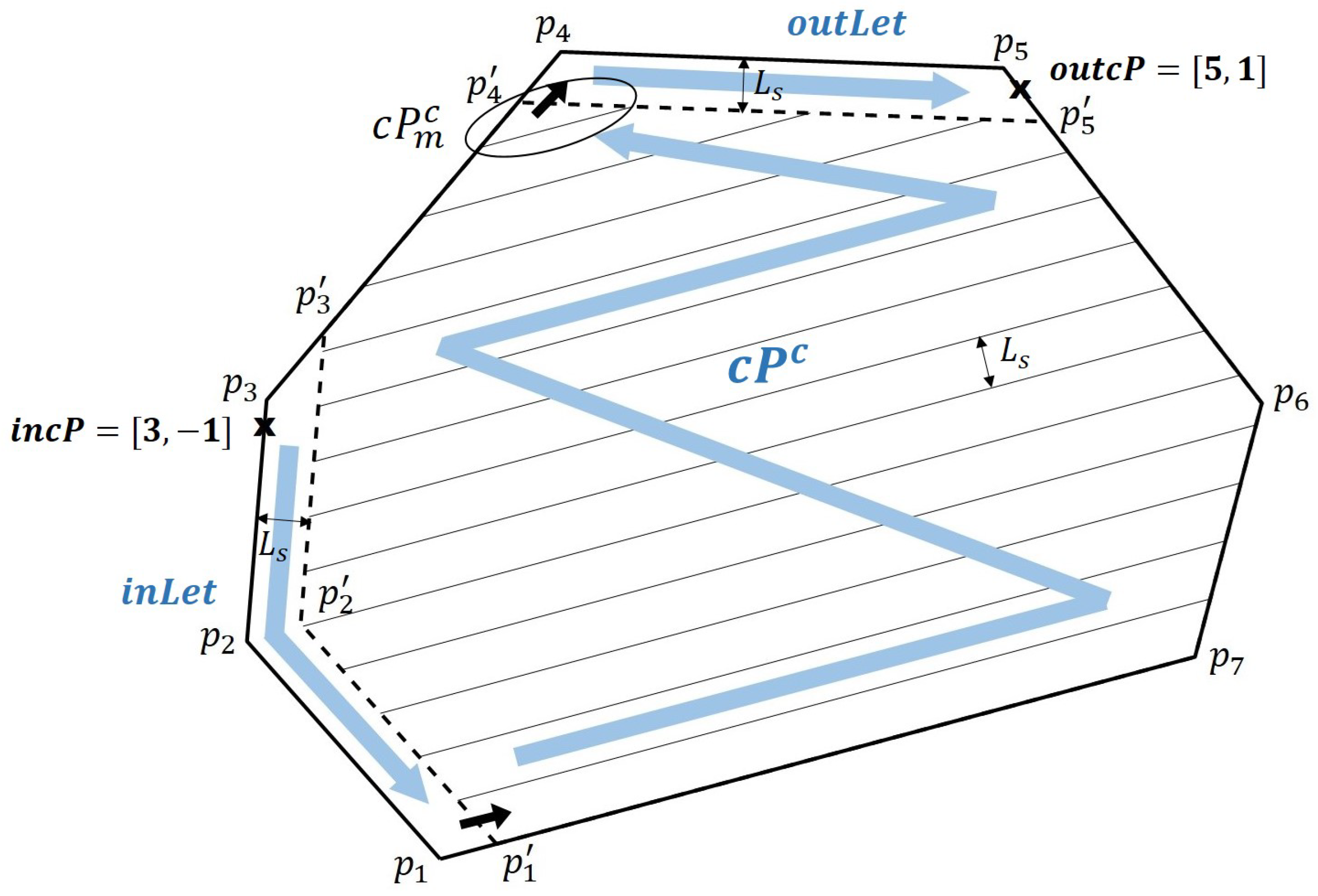
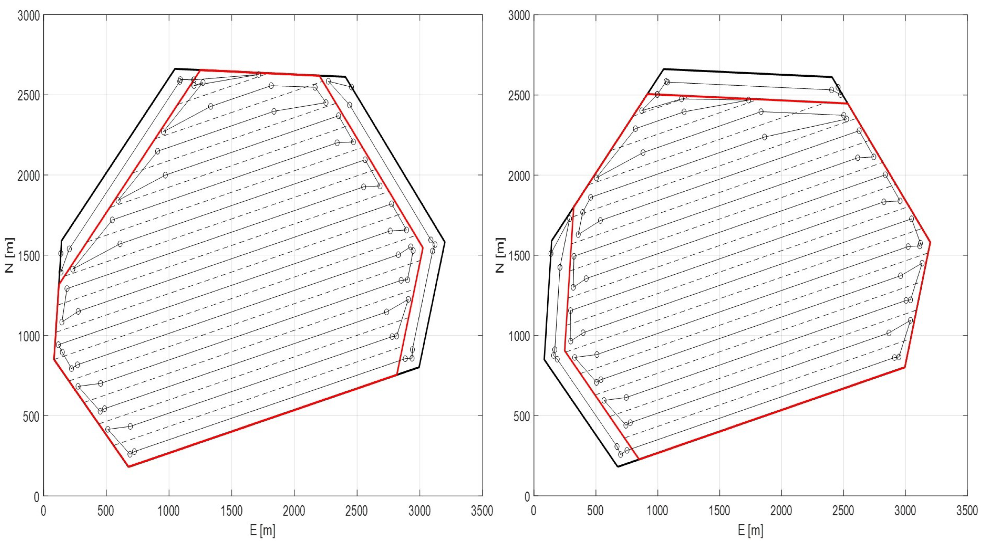
• To solve SP1 for any given $c\mathcal{P}$, the idea in this paper is simple that we pile the inter-tracks alongside a specific edge of $c\mathcal{P}$ so that we can cover $c\mathcal{P}$ with the minimum number of these inter-tracks.
• Apply CbSPSA to solve the SP2.
• Also, apply a method similar to CbSPSA combined with the circle whose radius is $r_m$ to round the path at each waypoint (solving SP3).

As mentioned before, the main contribution of this paper is to extend the results in the previous work [27] to the case where the vehicle has nonzero turning radius. In addition, some of the algorithms in [27] also have been upgraded in this paper, which can be further summarized as follows.

• Upgrade and more detailed description of Algorithm 2.
• Upgrade and detailed description of search algorithm for $c{\mathcal{P}}_m^c$, see Figure 1.

3.2. $c\mathcal{P}$ Partition: Solving SP1 and Some of SP2

For any given $c\mathcal{P}$, according to its definition, it is always monotone with respect to each of its edge [31]. For each edge $p_i{p}_{jmod(i-1,n)},i=1,\cdots ,n$, where $jmod$ is the same function of $mod$ except that $jmod(0,n)=n$, $h_{iM}$ denotes the maximum height among the vertices $p_j,j=i+1,\cdots ,jmod(i-2,n)$ to the edge $p_i{p}_{jmod(i-1,n)}$ [27]. Here we define $h_M=min\{h_{iM},i=1,\cdots ,n\}$, from which it is easy to verify that $ceil(h_M/Ls)$ is the minimum number of inter-tracks need to full cover the area $c\mathcal{P}$. Consequently, the strategy in this paper for the vehicle’s minimum turn number is straightforward that the vehicle is forced to search the area alongside the inter-tracks parallel to the edge corresponding to $h_M$ so that can minimize the vehicle’s turn numbers.

For the convenience of discussion, in this paper all convex polygons take the same form of $[p_1,\cdots ,p_n]$, where $p_1{p}_n$ is the edge corresponding to $h_M$. Indeed, this kind of expression is helpful to simplify the search algorithms proposed in this paper. In this case, we apply $tp=[m,1,n]$ to denote the specific vertices information for given $c\mathcal{P}$ [27], where $p_m$ is the vertex of $h_M$ to the edge $p_1{p}_n$. Moreover, for vertex $p_i$, if $1\le i<m$, then the vertex is said to be on the LEFT; otherwise, if $m<i\le n$, then it is on the RIGHT.

In this paper, the vehicle’s start and end points are all set at the polygon vertices. More specifically, the start point is set as $inc\mathcal{P}=[i,di{r}_i]$ and the end point is $outc\mathcal{P}=[j,di{r}_j]$ with $di{r}_i,di{r}_j=\pm 1$, $i,j=1,\cdots ,n$, where the exact position of $x=[k,di{r}_k],k=1,\cdots ,n$ is defined as following

$$x=p_k+0.5L_s[cos{\alpha }_k;sin{\alpha }_k]$$

(1)

where ${\alpha }_k=\angle p_i{p}_{jmod(i+di{r}_k,n)}$.

For any given $inc\mathcal{P}$ and $outc\mathcal{P}$, in order to avoid the possible occurrence of overlapped or crossed path, the polygon $c\mathcal{P}$ is further partitioned into three parts: $inLet$, $c{\mathcal{P}}^c$, and $outLet$, as seen in Figure 1. The rule of partition is that: (1) both the end of $inLet$ and the start waypoints of $outLet$ are connected to the one of vertices $p_{tp\left(i\right)},i\in \{1,2,3\}$; (2) if the end of $inLet$ is linked to $p_{tp\left(1\right)}$, then the start part of $outLet$ is to $p_{tp\left(2\right)}$ or $p_{tp\left(3\right)}$, and vice versa. For details of this partition will be discussed later.

According to the partition rule, the overall full coverage for $c\mathcal{P}$ can be constructed by

$$CP\left(c\mathcal{P}\right)=CP\left(inLet\right)+CP\left(c{\mathcal{P}}^c\right)+CP\left(outLet\right).$$

(2)

In order to guarantee the coverage path calculated through (2) to have the minimum turn numbers, we need the following condition to be satisfied.

Assumption A2.

Considering $c{\mathcal{P}}^c$ in Figure 1, its $t{p}^c$ is the same as $tp$ for $c\mathcal{P}$.

According to the partition rule, it is not difficult to verify that even in the case where the Assumption 2 is not satisfied, the maximum increasing turn number calculated through (2) will be less than 2 compared to the true minimum turn number. Therefore, in the case $h_M\gg L_s$, which is a very common in practice, whether Assumption 2 is true or not becomes less critical.

3.3. CbSPSA for $CP\left(c\mathcal{P}\right)$: Solving SP2

For any given $c\mathcal{P}$, according to the different locations of $inc\mathcal{P}$ and $outc\mathcal{P}$, there are different partition methods. At first, the different locations of $inc\mathcal{P}$ and $outc\mathcal{P}$ can be divided into two main categories: (1) both of them are on the same side (LEFT or RIGHT), (2) each on the other side. It is notable that in this paper we only consider the case where $inc\mathcal{P}$ and $outc\mathcal{P}$ are not on the same vertex. In the case (1), the partition method is straightforward that: if $inc\mathcal{P}$ is closer to $p_m$, then $inLet=inc\mathcal{P}\to p_m$ and $outLet=outc\mathcal{P}\to p_1$ (on the LEFT) or $p_n$ (on the RIGHT), and vice versa. In the latter case, also there are two different methods, one is $inLet=inc\mathcal{P}\to p_m$ and $outLet$ links to $p_1{p}_n$ and the other one is vice versa. However, in this case, it’s difficult to determine which one is best. In [27], the authors proposed a sort of selection law for an optimal partition of any given polygon through defining a criteria function Equation (4) as in [27]. This paper applies the similar way to choose the better partition of $inc\mathcal{P}$ and $outc\mathcal{P}$.

Consequently, according to (2), simply connecting the $CP\left(inLet\right)$, $CP\left(c{\mathcal{P}}^c\right)$, and $CP\left(outLet\right)$ at each of end and start points, we can search out the full CPP for $c\mathcal{P}$.

Algorithm 1 shows the overall flowchart of CbSPSA for any given convex polygon $c\mathcal{P}$. For given $c\mathcal{P}$, $searchSH\left(c\mathcal{P}\right)$ return $tp=[m,1,n]$, details of which are described in the previous Section 3.2. The function $carvePolygon(c\mathcal{P},tp,inc\mathcal{P},outc\mathcal{P})$ carries out the partition of $c\mathcal{P}$ as seen in (2) according to given $inc\mathcal{P}$ and $outc\mathcal{P})$. Usually, the result of $carvePolygon(\cdots )$ is not unique, instead it’s possible there are several different ways of partitions, among which we will choice the one with the shortest overall waypoint path length. For the remained functions $CP\left(inLet\right)$, $CP\left(outLet\right)$, and $Searc{h}_{c}Polygon(\cdots )$, they will be described in details in the following subsections.

Algorithm 1:  $Search\_Polygon(c\mathcal{P},inc\mathcal{P},outc\mathcal{P})$

Input: $c\mathcal{P},inc\mathcal{P},outc\mathcal{P}$,  Output:$CP\left(c\mathcal{P}\right)$ 1   $tp=searSH\left(c\mathcal{P}\right)$ 2   ${[c{\mathcal{P}}_i^c,inLe{t}_i,OutLe{t}_i]}_{i=1}^n=carvePolygon(c\mathcal{P},tp,inc\mathcal{P},outc\mathcal{P})$       3   for $i=1:n$ 4      $CP\left(c{\mathcal{P}}_i\right)\leftarrow \varnothing$ 5      $CP\left(c{\mathcal{P}}_i\right)\stackrel{add}{\leftarrow }CP\left(inLe{t}_i\right)$ 6      $CP\left(c{\mathcal{P}}_i\right)\stackrel{add}{\leftarrow }Searc{h}_{c}Polygon(c{\mathcal{P}}_i^c,inc{\mathcal{P}}_i^c,outc{\mathcal{P}}_i^c)$ 7      $CP\left(c{\mathcal{P}}_i\right)\stackrel{add}{\leftarrow }CP\left(outLe{t}_i\right)$ 8   end for 9   return The shortest path among $CP\left(c{\mathcal{P}}_i\right),i=1,\cdots ,n$

3.3.1. CbSPSA for $CP\left(inLet\right)$ and $CP\left(outLet\right)$

The search algorithms for $inLet$ and $outLet$ are the same except at the end point. At start and end points, the paths are searched using the function $calPoint31(x_1,x_2,\beta ,dir)$ as illustrated as in Figure 2, and at the intermediate vertices, using $calPoint32(x,\alpha ,\beta ,dir)$ which is depicted in Figure 3. It is notable that in the case of $inLet$, at the end point, the waypoints are still searched using $calPoint32(·)$.

3.3.2. CbSPSA for $CP\left(c{\mathcal{P}}^c\right)$

As depicted in Figure 1, $c{\mathcal{P}}^c$ consists of a number of trapezoids, in other words, inter-tracks. If the vehicle is allowed to move out of the search area as in the case of lawn mowing problem [5,6,7,17,18,19,20], then CPP problem becomes straightforward that we simply extend the each centerline to the outside of the search area and just link them one by one. Unfortunately, the vehicle is restricted to move inside the search area and also has nonzero turning radius. In this case, the key issues for CPP are as follows: (1) how to link the centerlines one-by-one in the corner areas, and (2) how to design a shortest pass to cover the area $c{\mathcal{P}}_m^c$. Accordingly, the proposed search algorithm CbSPSA for $CP\left(c{\mathcal{P}}^c\right)$ is presented as the pseudo-codes in Algorithms 2 and 3. For the convenience of discussion, in the algorithm we set $inc{\mathcal{P}}^c=[m^{\prime },\pm 1]$ and $outc{\mathcal{P}}^c=[1,+1]$ or $outc{\mathcal{P}}^c=[n,-1]$.

Algorithm 2:  $Search\_cPolygon(c{\mathcal{P}}^c,inc{\mathcal{P}}^c,outc{\mathcal{P}}^c)$

Input: $c{\mathcal{P}}^c,inc{\mathcal{P}}^c,outc{\mathcal{P}}^c$,  Output: $CP\left(c{\mathcal{P}}^c\right)$ 1   $CP\left(c{\mathcal{P}}^c\right)\leftarrow \varnothing$ 2   $n_c=ceil(h_M^{\prime }/L_s)$ 3   $LQ$:=$[p_{L1},p_{L2},\cdots ,p_{L{n}_c}]$,  $RQ$:=$[p_{R1},p_{R2},\cdots ,p_{R{n}_c}]$          4   for $i=1:n_c$ 5        if $i==1$ 6           Set $stat$ with $inc{\mathcal{P}}^c$, $outc{\mathcal{P}}^c$, and $n_c$ 7           $CP\left(c{\mathcal{P}}^c\right)\stackrel{add}{\leftarrow }Search\_cmPolygon(c{\mathcal{P}}_m^c,stat)$ 8        else 9           X:=last way point of $CP\left(c{\mathcal{P}}^c\right)$ 10          $CP\left(c{\mathcal{P}}^c\right)\stackrel{add}{\leftarrow }calPoint12(X,i,di{r}_i,LQ,RQ)$ 11          if $i<n_c$ 12               $CP\left(c{\mathcal{P}}^c\right)\stackrel{add}{\leftarrow }calPoint13(i,di{r}_i,LQ,RQ)$ 13          end if 14       end if 15   end for 16   return $CP\left(c{\mathcal{P}}^c\right)$

Algorithm 3:  $Search\_cmPolygon(c{\mathcal{P}}_m^c,stat)$

Input: $c{\mathcal{P}}_m^c,stat$,  Output: $CP\left(c{\mathcal{P}}_m^c\right)$ 1   $CP\left(c{\mathcal{P}}_m^c\right)\leftarrow \varnothing \stackrel{add}{\leftarrow }{x}_1:=inc{\mathcal{P}}_m^c=[m,stat\left[0\right]]$                 2   case 1. $stat\left[0\right]=+1$, $stat\left[1\right]=+1$ 3        $calPoints21(x_1,c{\mathcal{P}}_m^c,stat)$ 4   case 2. $stat\left[0\right]=+1$, $stat\left[1\right]=-1$ 5        $calPoints22(x_1,c{\mathcal{P}}_m^c,stat)$ 6   case 3. $stat\left[0\right]=-1$, $stat\left[1\right]=+1$ 7        $calPoints23(x_1,c{\mathcal{P}}_m^c,stat)$ 8   case 4. $stat\left[0\right]=-1$, $stat\left[1\right]=-1$ 9        $calPoints24(x_1,c{\mathcal{P}}_m^c,stat)$ 10   end case 11   return $CP\left(c{\mathcal{P}}_m^c\right)$

In Algorithm 2, the state variable $stat$ is defined as in

Table 1. Definition of the state variable $stat$.

Bytes	Values	Descriptions
$stat\left[0\right]$	$\pm 1$	Used to determine $inc{\mathcal{P}}_m^c=[m,stat\left[0\right]]$
$stat\left[1\right]$	$\pm 1$	Indicates the path direction. +1: $p_{L1}$ → $p_{R1}$, −1: $p_{R1}\to p_{L1}$.
$stat\left[2\right]$	1, 0	Indicates if there is a vertex between $p_{L1}$ and $p_m^{\prime }$ (clockwise). 1: yes, 0: no
$stat\left[3\right]$	1, 0	Indicates if there is a vertex between $p_m^{\prime }$ and $p_{R1}$ (clockwise). 1: yes, 0: no

and accordingly $c{\mathcal{P}}_m^c$ is constructed as $c{\mathcal{P}}_m^c=[p_{L1},p_2,p_m^{\prime },p_4,p_{R1}]$, where $p_2=p_{jmod(m-1,n)}^{\prime }$ if $stat\left[2\right]=1$ and $p_4=p_{jmod(m+1,n)}^{\prime }$ if $stat\left[3\right]=1$2. Also, the parameter $di{r}_i$ in the algorithm can be determined according to

Table 2. Determination of $di{r}_i$ in Algorithm 2.

$\mathit{outc}{\mathcal{P}}^{\mathit{c}}\left(1\right)$	${\mathit{n}}_{\mathit{c}}$	i	${\mathit{dir}}_{\mathit{i}}$
1	odd	odd	$R\to L$
1	odd	even	$L\to R$
1	even	odd	$L\to R$
1	even	even	$R\to L$
n	odd	odd	$L\to R$
n	odd	even	$R\to L$
n	even	odd	$R\to L$
n	even	even	$L\to R$

. Here it is worth to mention that, considering Figure 1 where $inLet$ is connected to $p_1^{\prime }$ of $c{\mathcal{P}}^c$ which is taken as $outc{\mathcal{P}}^c$ in the algorithm, the direction of $CP\left(c{\mathcal{P}}^c\right)$ should be reversed.

As mentioned before, one of main upgrade in this paper is that each waypoint of $CP\left(c\mathcal{P}\right)$ consists of $w{p}_i=(x_i,d_i)$ instead of $w{p}_i=x_i$ as in [27], where $x_i\in {\Re }^2$ is the horizontal position and the integer parameter $d_i$ indicates an additional information about $w{p}_i$. If $w{p}_i$ is located on the center line of inter-track, then we set $d_i=2$, otherwise $d_i=-2$. This kind of information will be used in the later smoothing process for $CP\left(c\mathcal{P}\right)$. On the other hand, in the algorithm, the function $calPoint12(·)$ is similar to $calPoints4(·)$ [27] and $calPoint13(·)$ is to $calPoints5(·)$ in [27], respectively. The difference is that the differentiation criteria is changed from $\alpha \ge \pi /2$ as in Figure 6 in [27] to $\alpha \ge 3\pi /2$. This is for the convenience of path smoothing for the vehicle’s nonzero turning radius, details of which will be discussed later.

The Algorithm 2 in [27] is also upgraded as follows. Here the detailed description of $calPoints21(·)$ and $calPoints22(·)$ are presented in Appendix A and Appendix B. This kind of detailed presentation is supposed to be of help for the readers’ in depth understanding of the proposed algorithm. The remainder of $calPoints23(·)$ is similar to $calPoints22(·)$ and $calPoints24(·)$ is to $calPoints21(·)$. The only difference is the search direction.

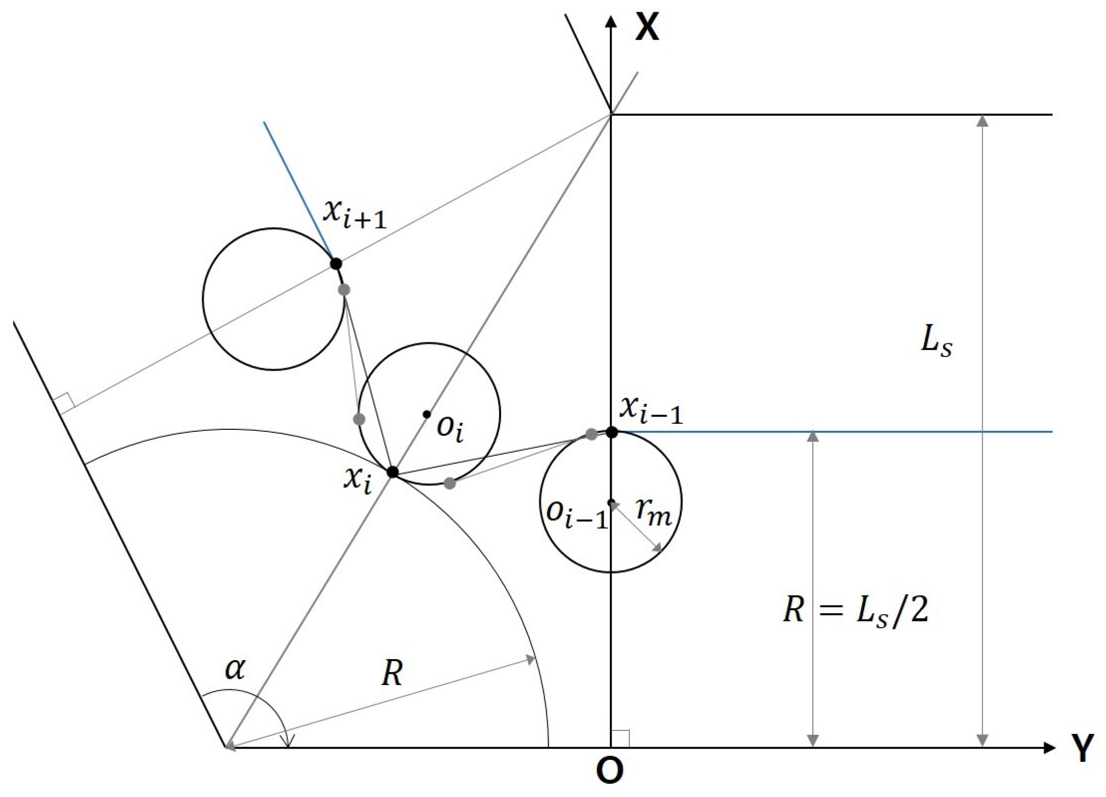
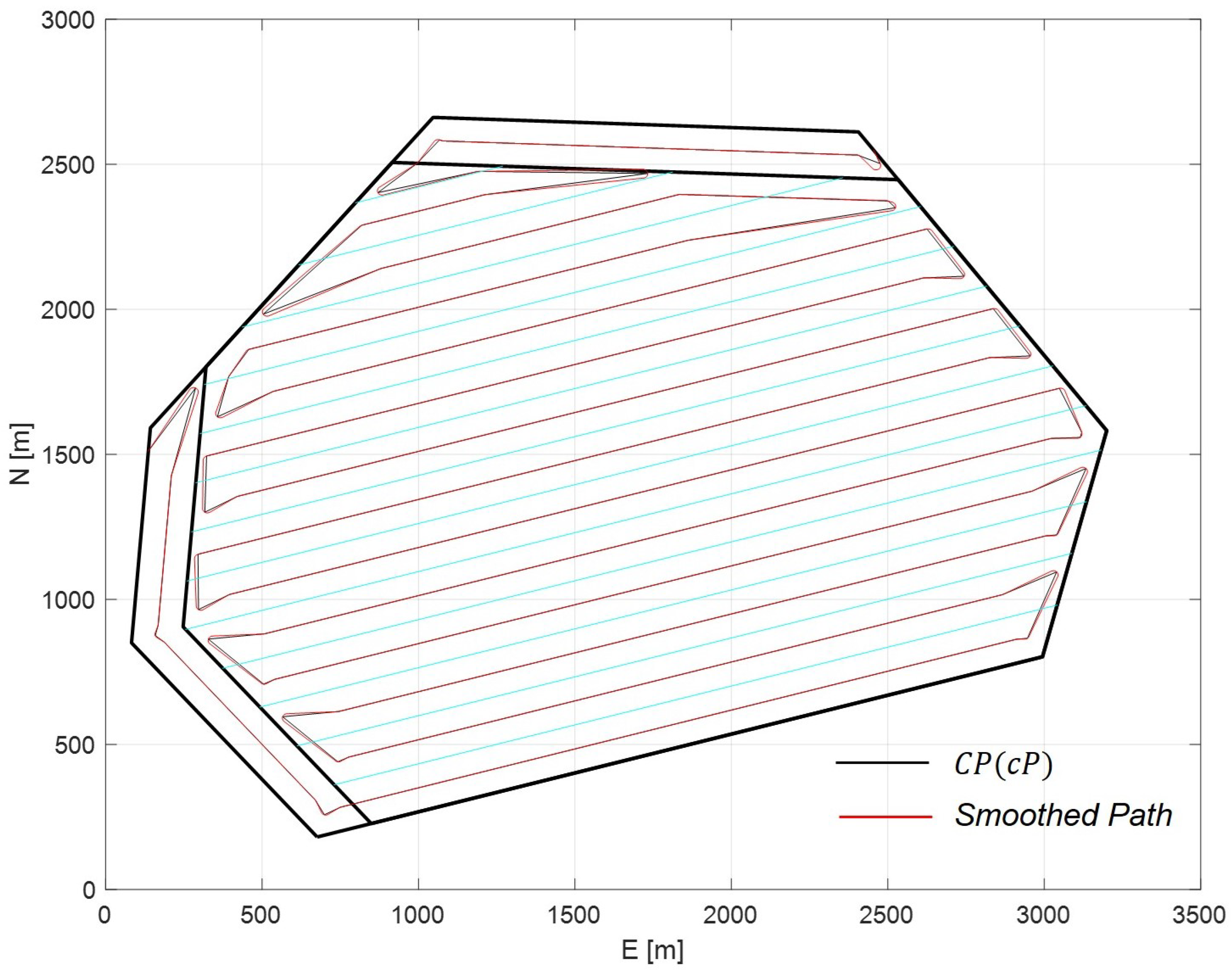
3.4. Smoothing $CP\left(c\mathcal{P}\right)$: Solving SP3

Here we recall some characteristics of $CP\left(c\mathcal{P}\right)$ searched by CbSPSA. For given $c\mathcal{P}$, since there are total of $n_c-1$ number of trapezoids, there are same number of center line pieces in $CP\left(c\mathcal{P}\right)$ [27], each of which corresponds to two adjacent waypoints. Therefore, there are total of $2(n_c-1)$ number of waypoints in $CP\left(c\mathcal{P}\right)$ on the center lines, and the remainder ones are not on these lines. This kind of information is encoded to the integer parameter in $w{p}_i=[x_i,d_i]$. $d_i=+2$ indicates $w{p}_i$ is on the center line, and $d_i=-2$ means it is not. Furthermore, each pair of adjacent waypoints are connected by straight lines [27]. In order for the vehicles, which have nonzero turning radius, to exactly follow it, this $CP\left(c\mathcal{P}\right)$ has to go through a specific smoothing process.

The smoothing process proposed in this paper is as the following Algorithm 4, and also depicted in Figure 4, Figure 5 and Figure 6. In the algorithm, the function $checkPoint(x,c\mathcal{P})$ is used to check if the point x is located inside the polygon $c\mathcal{P})$. If it is, then returns TRUE; otherwise, return FALSE. The integer parameter $d_i$ in $fCP\left(c\mathcal{P}\right)$ is encoded in different way. $d_i=1$ indicates the path from $w{p}_i$ is turning clockwise alongside the circle with $r_m$ the radius until the next waypoint, $d_i=-1$ means anticlockwise, and $d_i=0$ is the straightforward motion.

Algorithm 4:  $SmoothingPath\left(CP\right(c\mathcal{P}\left)\right)$

Input: $CP\left(c\mathcal{P}\right)$,  Output: $fCP\left(c\mathcal{P}\right)$ 1   $fCP\left(c\mathcal{P}\right)\leftarrow \varnothing \stackrel{add}{\leftarrow }(x_1,0)$ 2   for i = 2: (N − 1) 3        if $d_i==2$ 4           Calculate $x_i^{-}$ or $x_{i+1}^{+}$ as in Figure 5 5           $fCP\left(c\mathcal{P}\right)\stackrel{add}{\leftarrow }(x_i^{-},-1),(x_i,0)$ or $(x_{i+1},+1),(x_{i+1}^{+},0)$ 6        else if $d_i==-2$ 7           Calculate $x_i^{-}$ and $x_i^{+}$ according to Figure 5a 8           while(!$checkPoint(x_i^{-},c\mathcal{P})$)                 Increasing $\delta \alpha$ and calculate $x_i^{-}$ and $x_i^{+}$ according to Figure 5b       9           while(!$checkPoint(x_i^{+},c\mathcal{P})$)                 Increasing $\delta \alpha$ and calculate $x_i^{-}$ and $x_i^{+}$ according to Figure 5c       10          $fCP\left(c\mathcal{P}\right)\stackrel{add}{\leftarrow }(x_i^{-},-1),(x_i^{+},0)$ 11       end if 12   end for 13   $fCP\left(c\mathcal{P}\right)\leftarrow \varnothing \stackrel{add}{\leftarrow }(x_N,0)$ 14   return $fCP\left(c\mathcal{P}\right)$

There are some points need to be mentioned here. First, according to the Assumption 1, it is not difficult to verify that two points $x_i^{-}$ and $x_i^{+}$, as in the case of Figure 5, cannot be located outside of $c\mathcal{P}$ at the same time. And more interestingly, it is always possible for us to find out a proper value of $\delta \alpha$ so that both of $x_i^{-}$ and $x_i^{+}$ are all located inside $c\mathcal{P}$. Second, consider the case where one of $x_{i-1}$ and $x_{i+1}$ is located inside the circle3, see Figure 5. In this case, we can easily turn around the circle until the inside point is relocated outside the circle. For example, if $x_{i-1}$ is located inside the circle, then clockwise turning around the circle can easily relocate the point outside of it. Finally, let us consider an exceptional case as seen in Figure 3, which is the combination of Figure 4 and Figure 5. In this case, the path smoothing process can be depicted as in Figure 6, from which we can see that it seems possible that two circles $O(o_{i-1},r_m)$ and $O(o_i,r_m)$ can cross each other. In this case, it’s impossible to search out a path using Algorithm 4. With this in mind, in this paper we propose the following proposition.

Proposition 1.

Consider Figure 6. If $r_m$ satisfies $r_m\le (\sqrt{5}-2)R$, then we have $\left|\right|o_i{o}_{i-1}\left|\right|>2r_m$, $\forall \alpha \in [{\alpha }_{min},\pi )$.

Proof of Proposition 1.

See Appendix A. □

Here it’s notable that $r_m\le (\sqrt{5}-2)R$ is a kind of sufficient condition, not a necessary one. With this condition, we can guarantee that all the waypoints in $CP\left(c\mathcal{P}\right)$ can be properly smoothed so that the vehicle can exactly follow the path and further can guarantee the coverage path planning objective mentioned in Section 2 to be achieved.

4. Numerical Study

In this section, we carry out some of numerical simulations in MATLAB to further illustrate the effectiveness of the proposed path planning algorithm. In the simulation, we consider the convex polygon as $c\mathcal{P}=[p_1;p_2;p_3;p_4;p_5;p_6;p_7]=[181.2\mathrm{m}, 676.1\mathrm{m}; 850.4\mathrm{m},$ $82.7\mathrm{m}; 1591.2\mathrm{m}, 143\mathrm{m};$ $2661.6\mathrm{m}, 1046.8\mathrm{m}; 2611.7\mathrm{m}, 2406\mathrm{m}; 1582\mathrm{m}, 3199.6\mathrm{m}; 802.3\mathrm{m},$ ${2994.4\mathrm{m}]}^T$ with $incP=[3,-1]$ and $outcP=[5,1]$ as seen in Figure 1. For the parameters, the sonar swath is taken as $L_s=160\mathrm{m}$, and the vehicle’s minimum turn radius is set as $r_m=15\mathrm{m}$ so that can satisfy the condition in Proposition 1.

First, $tp=searchSH\left(c\mathcal{P}\right)$ returns $tp=[4,1,7]$, which means the height from the vertex $p_4$ to the edge $p_1{p}_7$ is the shortest. So the inter-track will be piled alongside $p_1{p}_7$. Then, we investigate the convex polygon partition method $carvePolygon(c\mathcal{P},tp,inc\mathcal{P},outc\mathcal{P})$. As mentioned before, since $inc\mathcal{P}=[3,-1]$ is located on LEFT side and $outc\mathcal{P}=[5,1]$ is on the RIGHT side, there are total of two partition methods, which means $i=1,2$ in Algorithm 1. Corresponding results are shown in Figure 7. In the left case, the total length of $CP\left(c\mathcal{P}\right)$ is 39,382 m and the total turn numbers4 are 18, and for right one, the length is 38,326 m and the turn numbers are 16. Therefore, Algorithm 1 return the coverage path as shown in right side in Figure 7. As for details of how to calculate the selection criteria for these two cases, refer to [27].

Now consider the path smoothing algorithm proposed in this paper. For the coverage path $CP\left(c\mathcal{P}\right)$ searched by Algorithm 1, we apply the smoothing method (Algorithm 4 in Section 3.4) and the corresponding result is shown in Figure 8. And Figure 9 shows some of the enlarged corner screen of Figure 8. From these results, we can see that the proposed smoothing method can provide a sort of satisfactory smoothing performance while can guarantee the result path all restricted inside the search area. Here it is worth to mention that in the case A as seen in Figure 9b, since $d_1{d}_2$, which is the common tangent between $c{\mathcal{P}}^c$ and $outLet$, is located inside the polygon $c\mathcal{P}$, the smoothed path has intersection with $d_1{d}_2$. In contrast, in the case of B as seen in Figure 9c, $d_3{d}_4$ is the edge of $c\mathcal{P}$, therefore the smoothed path has this kind of form so that to locate the path inside the polygon $c\mathcal{P}$.

Finally, Figure 10 shows the final sonar full coverage result after the vehicle finishes the trajectory following for given smoothed coverage path. Each green line indicates the sonar swath, and from Figure 10, we can see that the sonar swath fully covers the given polygon area $c\mathcal{P}$, while the vehicle keeps moving inside the polygon.

5. Conclusions

A full CPP method for marine survey where the vehicles have nonzero minimum turn radius has been presented in this paper. For any given convex polygon search area, it can be partitioned into three parts: $inLet$, $c{\mathcal{P}}^c$, and $outLet$. At each area, the coverage path is searched using proposed CbSPSA algorithm, and finally integrating these three path can easily construct the final waypoint path. For this straight line waypoint path, we have further proposed a smoothing algorithm so that for the vehicles with nonzero turning radius can exactly track the searched coverage path. Numerical analysis also has been carried out to illustrate the effectiveness of proposed schemes.

The current results are limited to the convex polygon and some of relatively simple polygon cases. How to extend these results to the case of more general form of polygon search areas might be one of our interesting future works. Also, it might be interesting to explore whether the current results can be easily extended to some of practical cases, such as marine surveys carried out by multiple AUVs and survey in 3D underwater space.

References

- Choset, H. Coverage for robotics—A survey of recent results. Ann. Math. Artif. Intell. 2001, 31, 113–126. [Google Scholar] [CrossRef]
- Galceran, E.; Carreras, M. A survey on coverage path planning for robotics. Robot. Auton. Syst. 2013, 61, 1258–1276. [Google Scholar] [CrossRef]
- Bormann, R.; Jordan, F.; Hampp, J.; Hagele, M. Indoor Coverage Path Planning: Survey, Implementation, Analysis. In Proceedings of the IEEE International Conference on Robotics and Automation, Brisbane, Australia, 21–25 May 2018; pp. 1717–1725. [Google Scholar]
- Taua, M.C.; Lisane, B.B.; Ferreira, R.R. Survey on Coverage Path Planning with Unmanned Aerial Vehicles. Drones 2019, 3, 4. [Google Scholar] [CrossRef]
- Arkin, E.M.; Fekete, S.P.; Mitchell, S.B. Approximation algorithms for lawn mowing and milling. Comput. Geom. 2000, 17, 25–50. [Google Scholar] [CrossRef]
- Huang, Y.Y.; Cao, Z.L.; Oh, S.J.; Kattan, E.U.; Hall, E.L. Automatic Operation for a Robot Lawn Mower. SPIE Conf. Mob. Robot. 1987, 727. [Google Scholar] [CrossRef]
- Hofmann, M.; Clemens, J.; Stronzek-Pfeifer, D.; Simonelli, R.; Serov, A.; Schettino, S.; Runge, M.; Schill, K.; Buskens, C. Coverage Path Planning and Precise Localization for Autonomous Lawn Mowers. In Proceedings of the 6th IEEE International Conference on Robotic Computing, Naples, Italy, 5–7 December 2022; pp. 238–242. [Google Scholar]
- Vosniakos, G.; Papapanagiotou, P. Multiple tool path planning for NC machining of convex pockets without islands. Robot. Comput. Integr. Manuf. 2000, 16, 425–435. [Google Scholar] [CrossRef]
- Chen, X.; Tucker, T.T.; Kurfess, T.R.; Vuduc, R.; Hu, L. Max orientation coverage: Efficient path planning to avoid collisions in the CNC milling of 3D objects. In Proceedings of the 2020 IEEE/RSJ International Conference on Intelligent Robots and Systems, Las Vegas, NV, USA, 24 October 2020–24 January 2021; pp. 6862–6869. [Google Scholar]
- Held, M. On the Computational Geometry of Pocket Maching; Lecture Notes in Computer Science; Springer: New York, NY, USA, 1991; Volume 500. [Google Scholar]
- Dhanik, S.; Xirouchakis, R. Contour parallel milling tool path generation for arbitrary pocket shape using a fast marching method. Int. J. Adv. Manuf. Technol. 2010, 50, 1101–1111. [Google Scholar] [CrossRef]
- Venkatesh, R.; Vijayan, V.; Parthiban, A.; Sathish, T.; Chandran, S.S. Comparison of different tool path pocket milling. Int. J. Mech. Eng. Technol. 2018, 9, 922–927. [Google Scholar]
- Yasutomi, F.; Yamada, M.; Tsukamoto, K. Cleaning robot control. In Proceedings of the IEEE International Conference on Robotics and Automation, Philadelphia, PA, USA, 24–29 April 1988; pp. 1839–1841. [Google Scholar]
- Hofner, C.; Schmidt, G. Path planning and guidance techniques for an autonomous mobile cleaning robot. Robot. Auton. 1995, 14, 199–212. [Google Scholar] [CrossRef]
- Prassler, E.; Ritter, A.; Schaeffer, C.; Fiorini, P. A Short History of Cleaning Robots. Auton. Robot. 2000, 9, 211–226. [Google Scholar] [CrossRef]
- Miao, X.; Lee, J.; Kang, B.Y. Scalable Coverage Path Planning for Cleaning Robots Using Rectangular Map Decomposition on Large Environments. IEEE Access 2018, 6, 38200–38215. [Google Scholar] [CrossRef]
- Acar, E.U.; Choset, H.; Zhang, Y.; Schervish, M. Path Planning for Robotic Demining: Robust Sensor-based Coverage of Unstructured Environments and Probabilistic Methods. Int. J. Robot. Res. 2003, 22, 441–466. [Google Scholar] [CrossRef]
- Seder, M.; Petrovic, I. Complete coverage path planning of mobile robots for humanitarian demining. Ind. Robot. 2012, 39, 484–493. [Google Scholar]
- Stoll, A.; Kutzbach, D. Guidance of a Forage Harvester with GPS. Precis. Agric. 2000, 2, 281–291. [Google Scholar] [CrossRef]
- Oksanen, T.; Visala, A. Coverage Path Planning Algorithms for Agricultural Field Machines. J. Field Robot. 2009, 26, 651–668. [Google Scholar] [CrossRef]
- Wong, S.C.; MacDonald, B.A. A topological coverage algorithm for mobile robots. In Proceedings of the IEEE/RSJ International Conference on Intelligent Robots and Systems, Las Vegas, NV, USA, 27–31 October 2003; pp. 1685–1690. [Google Scholar]
- Tang, J.; Sun, C.; Zhang, X. MSTC*: Multi-robot Coverage Path Planning under Physical Constraints. In Proceedings of the 2021 IEEE International Conference on Robotics and Automation, Xi’an, China, 30 May–5 June 2021; pp. 2518–2524. [Google Scholar]
- Paull, L.; Saeedi, S.; Seto, M.; Li, H. Sensor-Driven Online Coverage Planning for Autonomous Underwater Vehicles. IEEE/ASME Trans. Mechatronics 2013, 18, 1827–1838. [Google Scholar] [CrossRef]
- Sun, B.; Zhu, D.; Tian, C.; Luo, C. Complete Coverage Autonomous Underwater Vehicles Path Planning Based on Glasius Bio-Inspired Neural Network Algorithm for Discrete and Centralized Programming. IEEE Trans. Cogn. Dev. Syst. 2019, 11, 73–84. [Google Scholar] [CrossRef]
- Yordanova, V.; Gips, B. Coverage Path Planning With Trackn Spacing Adaptation for Autonomous Underwater Vehicles. IEEE Robot. Autom. Lett. 2020, 5, 4774–4780. [Google Scholar] [CrossRef]
- Bagnitckii, A.; Inzartsev, A.; Pavin, A. Planning and correction of the AUV coverage path in real time. In Proceedings of the 2017 IEEE Underwater Technology, Busan, Republic of Korea, 21–24 February 2017. [Google Scholar] [CrossRef]
- Li, J.H.; Kang, H.; Kim, M.G.; Jin, H.; Lee, M.J.; Cho, G.R.; Bae, C. Full Coverage of Confined Irregular Polygon Area for Marine Survey. IEEE Access 2023, 11, 92200–92208. [Google Scholar] [CrossRef]
- Stefan, H.; Kurt, M. Fast triangulation of simple polygons. In Foundations of Computation Theory; Lecture Notes in Computer Science; Springer: Berlin/Heidelberg, Germany, 1983; Volume 158, pp. 207–218. [Google Scholar]
- Li, J.H. 3D trajectory tracking of underactuated non-minimum phase underwater vehicles. Automatica 2023, 155, 111149. [Google Scholar] [CrossRef]
- Fossen, T.I. Guidance and Control of Ocean Vehicles; John Wiley & Sons Ltd.: Chichester, UK, 1994. [Google Scholar]
- Heckbert, P.S. Testing the Convexity of a Polygon; Academic Press: London, UK, 1994. [Google Scholar]