A Method for Estimating the Distribution of Trachinotus ovatus in Marine Cages Based on Omnidirectional Scanning Sonar

Abstract

In order to accurately estimate the distribution of Trachinotus ovatus in marine cages, a novel method was developed using omnidirectional scanning sonar and deep-learning techniques. This method involved differentiating water layers and clustering data layer by layer to achieve precise location estimation. The approach comprised two main components: fish identification and fish clustering. Firstly, omnidirectional scanning sonar was employed to perform spiral detection within marine cages, capturing fish image data. These images were then labeled to construct a training dataset for an enhanced CS-YOLOv8s model. After training, the CS-YOLOv8s model was used to identify and locate fish within the images. Secondly, the cages were divided into water layers with depth intervals of 40 cm. The identification coordinate data for each water layer were clustered using the DBSCAN method to generate location coordinates for the fish in each layer. Finally, the coordinate data from all water layers were consolidated to determine the overall distribution of fish within the cage. This method was shown, through multiple experimental results, to effectively estimate the distribution of Trachinotus ovatus in marine cages, closely matching the distributions detected manually.

1. Introduction

Cage aquaculture is the main aquaculture mode for the development of modern marine pastoralism [1], playing an indispensable role in the conservation and utilization of marine resources. To ensure culture efficiency and fish health, simply estimating the distribution of fish in the marine cages is insufficient for a comprehensive understanding of the state of aquaculture [2,3]. The distribution of fish in marine cage, especially at different time periods and in different areas, is important for optimizing feeding management, preventing disease outbreaks, and improving culture efficiency [4]. Firstly, the distribution of fish in the marine cage at different time periods is affected by a variety of factors that are not, or are only partially, controllable in open sea cages by aquaculture managers; these include daylight, temperature [5], feed placement time, waves [6], and other environmental conditions. Understanding these distribution patterns is useful for aquaculture managers to determine when fish reach satiation during feeding, so that they can adjust feeding strategies, such as optimizing the timing and location of feed placement, thereby improving feed utilization and reducing waste. Secondly, understanding the spatial distribution of fish helps to identify normal and abnormal behavior, serving as an indicator of sub-optimal rearing conditions or good management practices. Dense fish populations are more likely to lead to increased stress, skin or fin damage, and the rapid spread of diseases. By understanding the spatial distribution of fish and adjusting high-density areas, the risk of disease is effectively reduced [7]. Therefore, accurately estimating the distribution of fish in marine cage culture is an important challenge [8].

The estimation methods for the distribution of fish in cages mainly include three categories: acoustic, optical, and acousto-optical methods [9]. However, acousto-optical devices are too expensive, and the implementation conditions and steps are too cumbersome. Therefore, the current mainstream methods are acoustic and optical methods. Optical methods have advantages such as non-invasiveness and high resolution [10]. Some scholars have proposed methods of monitoring and estimation with different optical devices and have achieved good results [11,12,13]. Under seawater, optical devices have low visibility; the close-range resolution is high, but the long-range resolution is low. The resolution is also very low when the seawater is turbid. Therefore, it is difficult to fully exploit the advantages of optical methods. By contrast, the detection range of acoustic methods is larger, and the resolution is more constant. Data can be acquired with various sonar devices to generate image information and obtain data on the fish in marine cages [14]. In recent years, the utilization of sonar devices has achieved some positive results in the monitoring of fishery resources [15,16,17,18,19]. Feng et al. [20] proposed an automatic estimation method for fish abundance in sonar images. This method was based on an improved multi-column convolutional neural network (MCNN) and supplemented by multi-expansion rate fusion loss, improving the accuracy of the model and enhancing the level of information technology in aquaculture. Duffy et al. [21] used side-scan sonar and underwater video to draw sediment maps of reefs near the northern coast of Illinois in Lake Michigan to describe and quantify the distribution of lake trout and the eggs laid. Jing et al. [22] used DIDSON imaging sonar to obtain water data, calculate the average density of objects, and estimate the quantity of fish in the water in combination with the water area. This method also had high statistical accuracy. Chevallay et al. [23] combined small sonar tags with active acoustic and high-resolution GPS, pressure, motion, and optical sensors to explore the oceanographic parameters and distribution of seal-aimed pelagic fish and the behaviors of seals. Cui et al. [24] proposed a fish quantity estimation method based on imaging sonar. In this method, denoising, edge extraction, object segmentation, and other treatments were performed on the data acquired by the sonar to determine the image features of fish. Afterward, the measurement area of the sonar was counted to calculate the average volume density and realize the estimation of fish quantity in combination with the area of the culture area. The above studies have shown that monitoring fish with sonar is efficient and convenient. However, the opening angle problem of the sonic wave of the sonar during operation results in a limited scanning area and the existence of visual blind spots in the detected data, leading to double counting or the missed counting of fish. This has a significant influence on the estimation of fish distribution. Therefore, solving the visual blind spots during sonar measurement needs to be further explored to estimate fish distribution more accurately.

In summary, this study proposes a method for fish distribution estimation in marine cage aquaculture based on omnidirectional scanning sonar. This method mainly involves fish identification and counting as well as fish clustering. The method achieves distribution estimation through water layer differencing and column-by-column clustering, which not only estimates the number of fish in aquaculture cages but also provides detailed information about fish distribution. This detailed information could offer effective data support for improving aquaculture efficiency and management levels.

2. Materials and Methods

2.1. Experimental Materials and Collection

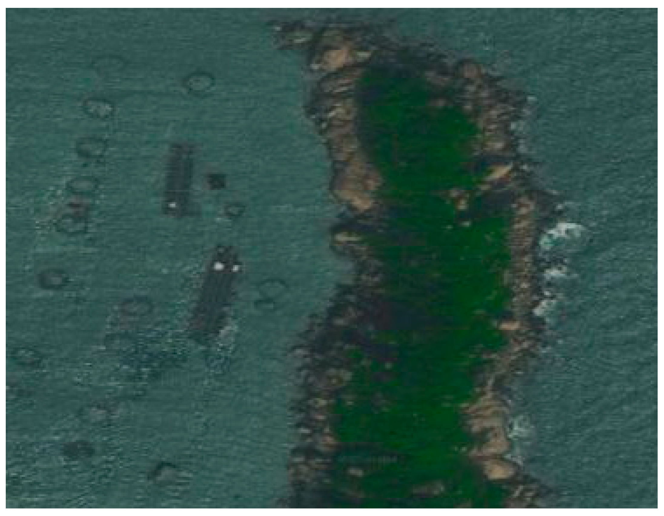
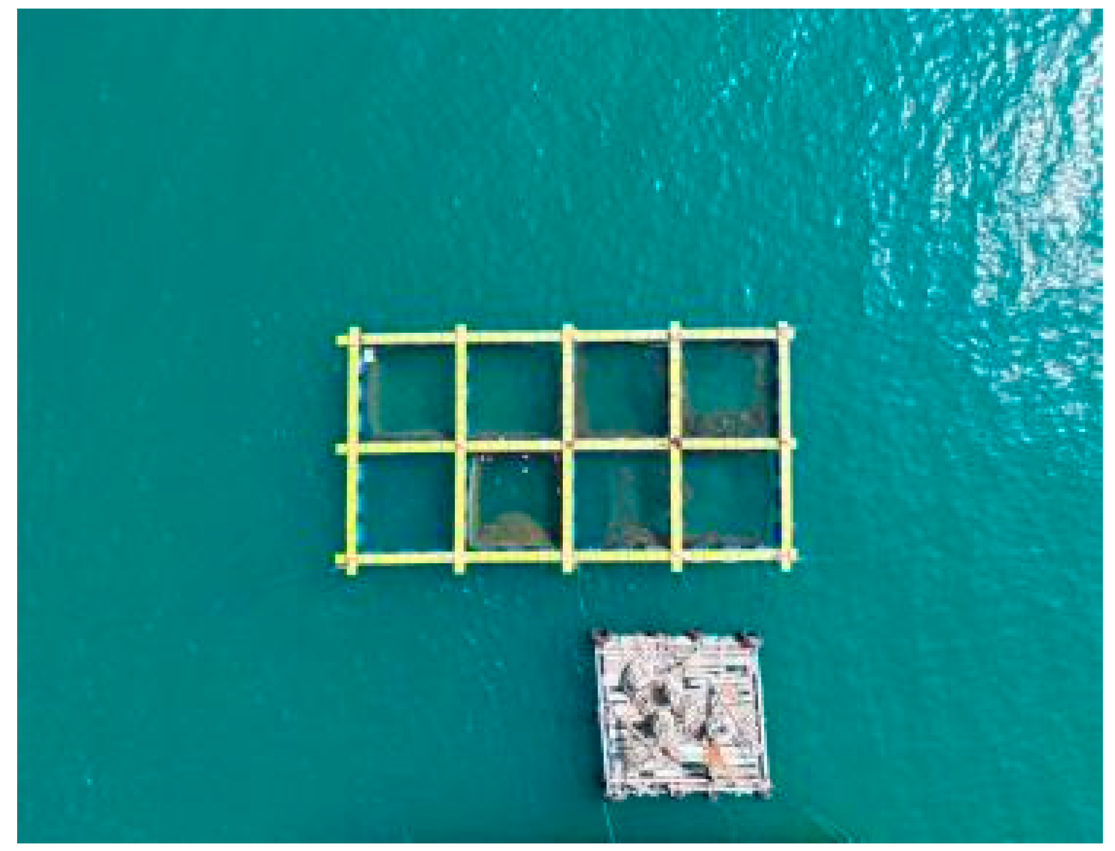
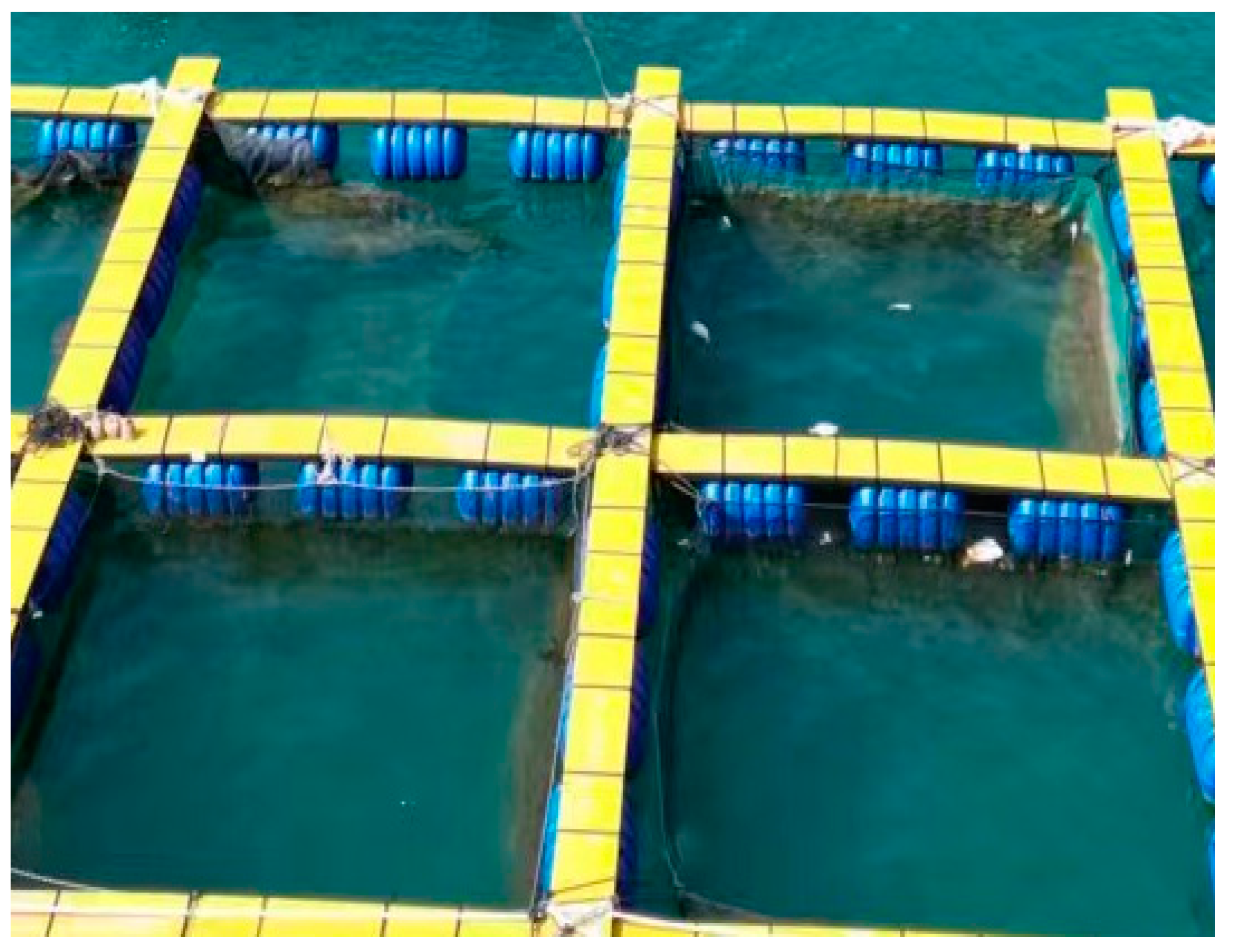
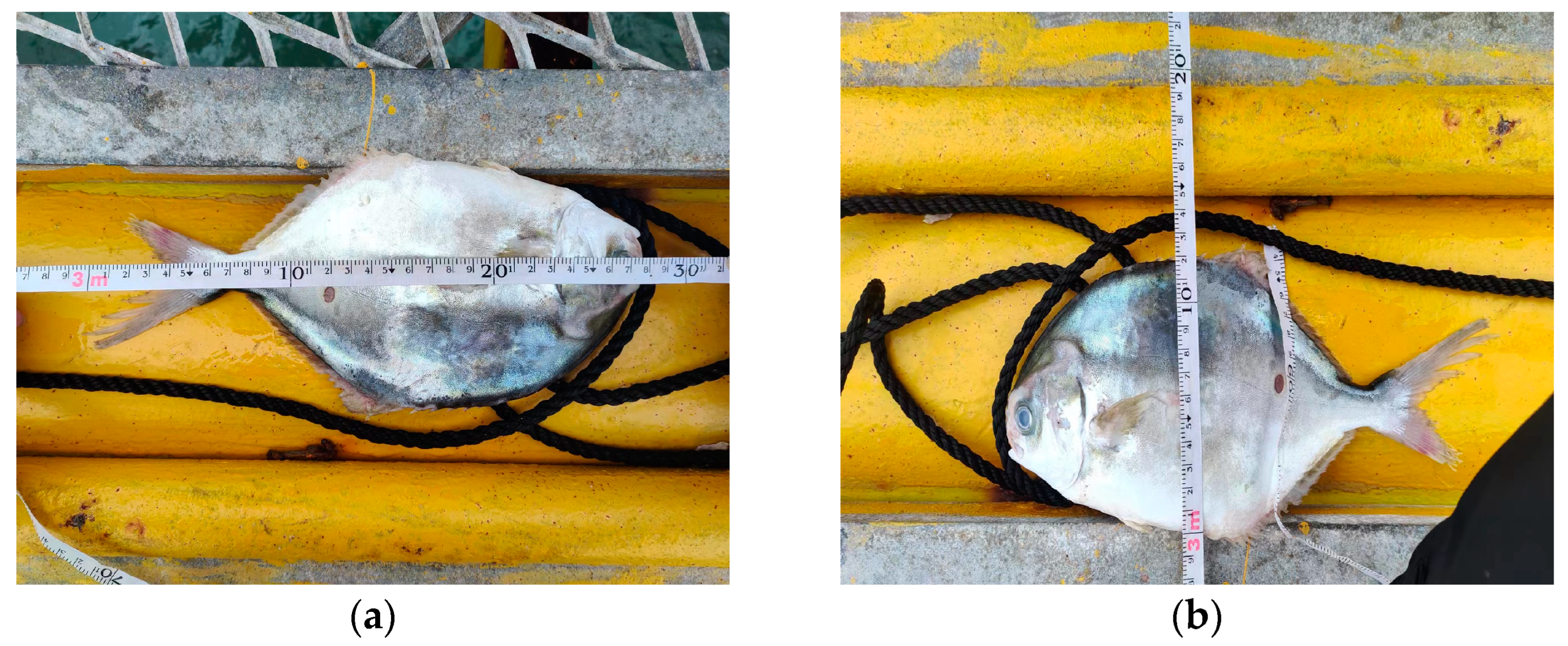
2.1.1. Experimental Site and Biological Samples

The experimental data were measured and obtained in the adjacent waters of Guishan Island, Zhuhai, Guangdong province (113.84473° E, 22.12571° N, salinity 21.5‰ and visibility of approximately 1.5 m) on 7 January, 2024. The satellite map of the experimental area and the aerial view of the experimental site are shown in Figure 1 and Figure 2, respectively.

The cage used in this experiment is shown in Figure 3. The dimensions of the cage are 4 m × 4 m × 4 m. The four corners of the cage had additional weights to ensure that it remained stable underwater. However, affected by the buoyancy of seawater, the depth of the cage was approximately 2.9 m. The fish used in this experiment were Trachinotus ovatus under normal culture conditions. The body length of the fish was approximately 24 cm (Figure 4).

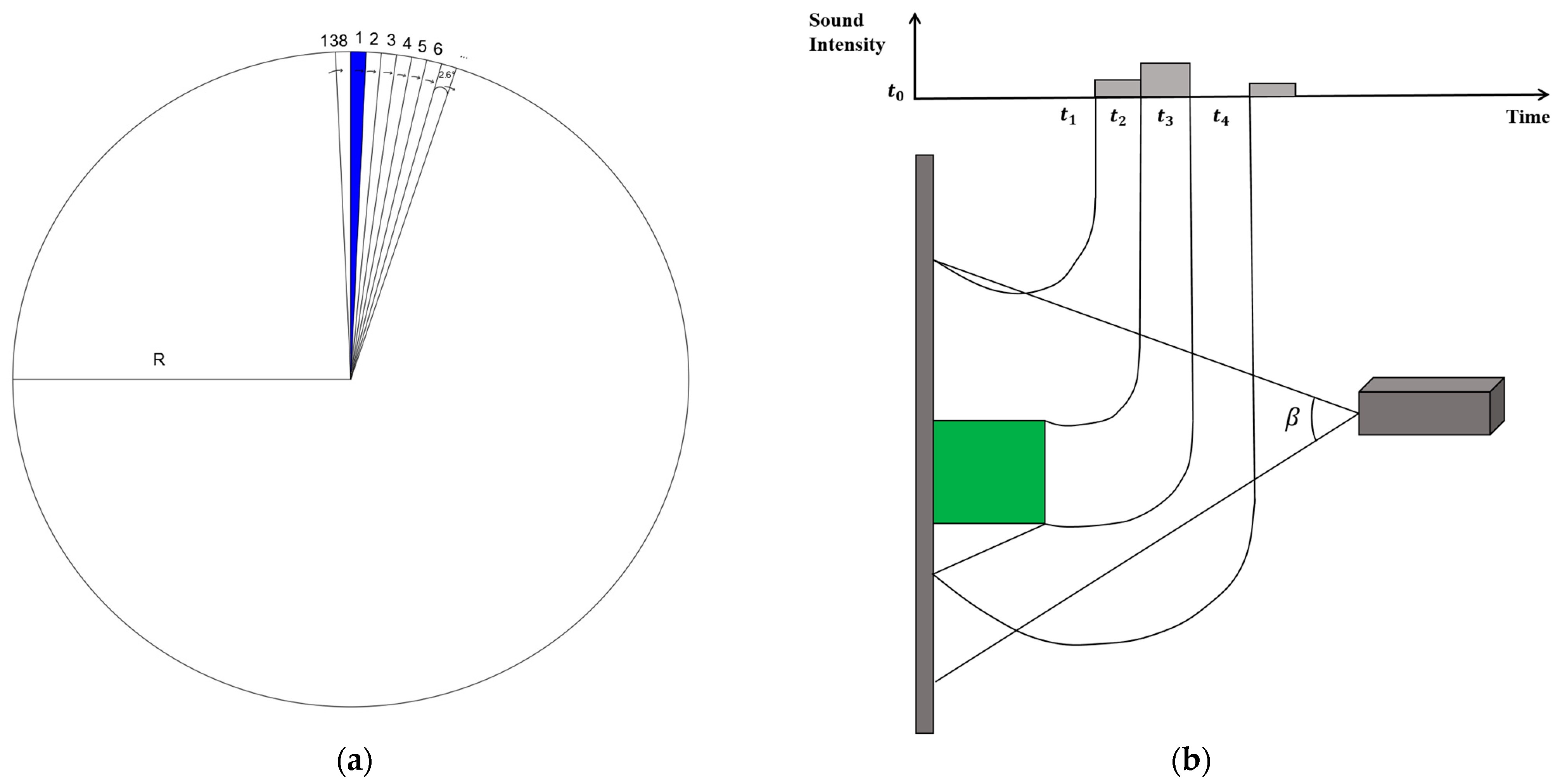
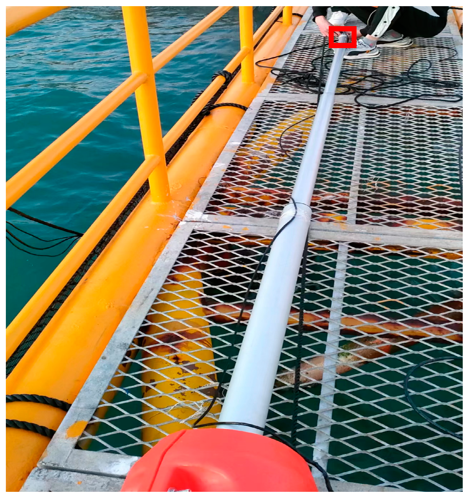
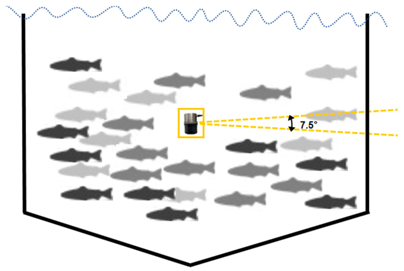
2.1.2. Device and Operating Mode

The device used in this paper was the omnidirectional scanning imaging sonar Scanfish-II (A2), launched by T-SEA Marine Technology Co., Ltd. (Zhangjiagang, China) This small imaging sonar was designed for underwater detection. Its specific technical indexes are shown in

Table 1. Technical indexes of high-frequency horizontal mechanical scanning sonar.

Item	Technical Index
Operating frequency	667 kHz
Range of action	3 m
Beam opening angle(Vertical × Horizontal)	$(7.5\pm 1.5)°\times (2.6\pm 0.3)°$
Distance pixel/precision	5 cm
Scanning area (polar coordinates)	360°
Maximum working depth	3 m
Pan tilt rotation frequency	2.5 s/circle
Cylinder size	$\mathsf{\Phi }$57 mm × 99 mm

.

The working principle of the sonar is shown in Figure 5a. The range of the sonar is denoted as R, with a beam opening angle of 2.6° horizontally and 7.5° vertically. The sonar emits ultrasonic waves, and the beam is rotated sequentially through the gimbal to achieve 360° horizontal measurement.

In the measurement of each detection angle, the sonar emits a sound signal forward, and the echo signal reflected from the target object within the beam’s irradiation area is received by the sonar for imaging. The detection beam emitted by the sonar is horizontally divided into several fan-shaped beams with vertical opening angles. Each beam illuminates the target, as shown in Figure 5b, forming a set of distance and intensity information. The echo intensity information of all beams is arranged based on position relationship to create the sonar image. The intensity of the echo signal reflects the acoustic reflection characteristics of different target objects, while the resulting time delay is used to determine the actual distance of the target object relative to the sonar position.

2.1.3. Data Acquisition

This experiment was a quantitative and temperature study that compared different quantities and culture temperatures of Trachinotus ovatus, with a difference of 50 fish in each group. Two hundred of the tens of thousands of fish cultured in the same batch were caught for the experiment, so there was no great disparity between the individual fish.

The sonar is shown in Figure 6, and it was designed to be connected to the end of the silver electric telescopic rod depicted in Figure 7. The telescopic rod drove the sonar to achieve unidirectional, uniform, vertical movement. Both the telescopic rod and the sonar were connected to 24 V batteries for their power supply. The maximum telescopic speed of the rod was 2.8 cm·s⁻¹, with a maximum range (fully extended) of 6.41 m (allowing access to the bottom of the cage), a fixed length (not extended) of 1.5 m, and a telescopic capacity of 4.9 m. The rod was supported by an orange float to keep it suspended above the water surface. The omnidirectional scanning sonar was used for underwater measurement, and the data were transmitted back to the computer. The sonar operated in low-frequency mode, and the range was set to 3 m, based on the maximum radius of the cage (approximately 2.8 m).

The steps for a single data collection were as follows: Suspend the telescopic rod with the sonar at the center of the water surface of the cage, ensuring the sonar is in contact with the water surface. Activate both the sonar and the electric telescopic rod. The telescopic rod drives the sonar to move underwater at a constant speed of 2.4 cm/s for measurement. The telescopic rod should stop working when its extension length (from the water surface to the bottom of the sonar) reaches 2.9 m, which is the maximum depth affected by buoyancy in the cage. This measurement depth is recorded as experimental data. The sonar data are recorded at 160 frames per second, with each recording lasting approximately 2 min. After the data acquisition, retrieve the sonar to the water surface. Note: As shown in Figure 8, the sonar was positioned on the center axis of the cage. During the scanning operation, the telescopic rod was extended so that the sonar moved at a uniform speed along the center axis in a unidirectional manner. Consequently, the scanning area was not limited to the horizontal plane but formed a spiral measurement pattern.

In order to explore the effects of temperature on fish distribution in sea cages, we designed an experimental scheme. Firstly, at 8:00 (approximately 16 degrees Celsius), 100 fish were manually removed from the right side of the experimental cages, as shown in Figure 3, and placed in the cage for the experiment. The previous collection steps were repeated and the experimental data were recorded. Next, another 50 fish were manually placed into the cage, bringing the total fish to 150. The previous collection procedure was then repeated to collect the experimental data. Finally, another 50 fish were added to the cage to bring the total fish to 200. The collection procedure was repeated to collect the experimental data. We waited until 13:00 (approximately19 degrees Celsius) and repeated the collection procedure. Data were collected for three different numbers of fish at this time. At 18:00 (approximately 18 degrees Celsius), the collection procedure was repeated. Data were collected for three different numbers of fish at this time. A total of 19 sets of experimental data were collected.

The 19 groups of data were numbered; 7 groups of data with 200 tails were numbered as 13, 14, 15, 16, 17, 18, 19; 6 groups of data with 100 tails were numbered as 1, 2, 3, 4, 5, 6; and 6 groups of data with 150 tails were numbered as 7, 8, 9, 10, 11, 12. Of these, numbers 1, 2, 7, 8, 13, and 14 are 8:00 data; numbers 3, 4, 9, 10, 15, and 16 are 13:00 data; and numbers 5, 6, 11, 12, 17, 18, and 19 are 18:00 data.

At each time period, the number of fish in each group was measured two times, with one randomly selected as the training group for the target recognition model and the other as the test group.

2.2. Data Saving Method

The image data, collected 19 times by the sonar, were replayed and processed to obtain video format image data for subsequent target recognition using a trained recognition model. There was a total of 19 sets of video data. Each set of data corresponded to the time per second of the sonar during spiral measurement, with a duration of approximately 2 min and a resolution of 804 pixels in width by 604 pixels in height.

2.3. Object Identification Module

2.3.1. Identification Model CS-YOLOv8s

The YOLOv8 model by Ultralytics is a SOTA model based on previous YOLO versions [25]. On the premise of maintaining real-time performance and high detection accuracy, this paper proposes an improved object detection model, CS-YOLOv8s, based on the YOLOv8s model.

Considering that each fish in sonar images is a small object, the core idea of the improved algorithm was to enhance the network’s ability to perceive the feature information of small objects. CS-YOLO focuses on optimizing the structure of the original model and introduces the CoT attention mechanism [26] to improve small object detection. Additionally, redundant information is processed using the thin neck module of Slim-Neck [27], and the GSConv [27] model is integrated to enhance the model’s identification performance while maintaining a lightweight design.

2.3.2. Dataset Creation

The sonar image data obtained were recorded as video data, with each second corresponding to each second during the spiral measurement. From this image data, 200 fish sonar images were randomly captured and annotated with MakeSense (category—fish). The annotated datasets were then randomly divided into two categories: 160 images were used as training sets, and 40 images were used as test sets.

2.3.3. Evaluation Indexes

Evaluation indexes are essential for assessing model performance. To evaluate the effectiveness of the proposed method, this study focused on four measures: Params, GFLOPs, mAP, and Size. GFLOPs indicate the amount of computation required by the model, reflecting its complexity. Params describe the number of parameters contained in the model.

The specific type of Average Precision (AP), referred to as mAP (mean Average Precision), was obtained by sorting the predicted values and the recall values of the model [25]. It involved calculating the area enclosed by the lines generated by the vertical axis and the recall values represented on the horizontal axis in the Cartesian coordinate system. This area provided a measure of the model’s precision and recall performance across different thresholds.

$$\mathrm{A}\mathrm{P}=\sum _{\mathrm{n}}({\mathrm{R}}_{\mathrm{n}+1}-{\mathrm{R}}_{\mathrm{n}})·{\mathrm{P}}_{\mathrm{n}}$$

(1)

where R is Recall, the recall represented by the horizontal axis; P is Precision, the precision represented by the vertical axis.

[email protected] refers to the value of Average Precision (AP) when the Intersection over Union (IoU) threshold is set at 0.5 and [email protected]:0.95 represents the mean Average Precision across IoU thresholds ranging from 0.5 to 0.95 in increments of 0.05 [25]. There is a positive correlation between the precision of the model and the mAP [25].

$$\mathrm{m}\mathrm{A}\mathrm{P}@0.5:0.95\mathrm{\%}={\displaystyle \frac{{\mathrm{A}\mathrm{P}}_{\mathrm{I}\mathrm{o}\mathrm{U}=0.5}+{\mathrm{A}\mathrm{P}}_{\mathrm{I}\mathrm{o}\mathrm{U}=0.55}+...+{\mathrm{A}\mathrm{P}}_{\mathrm{I}\mathrm{o}\mathrm{U}=0.95}}{\mathrm{n}}}$$

(2)

where the value of n was 10.

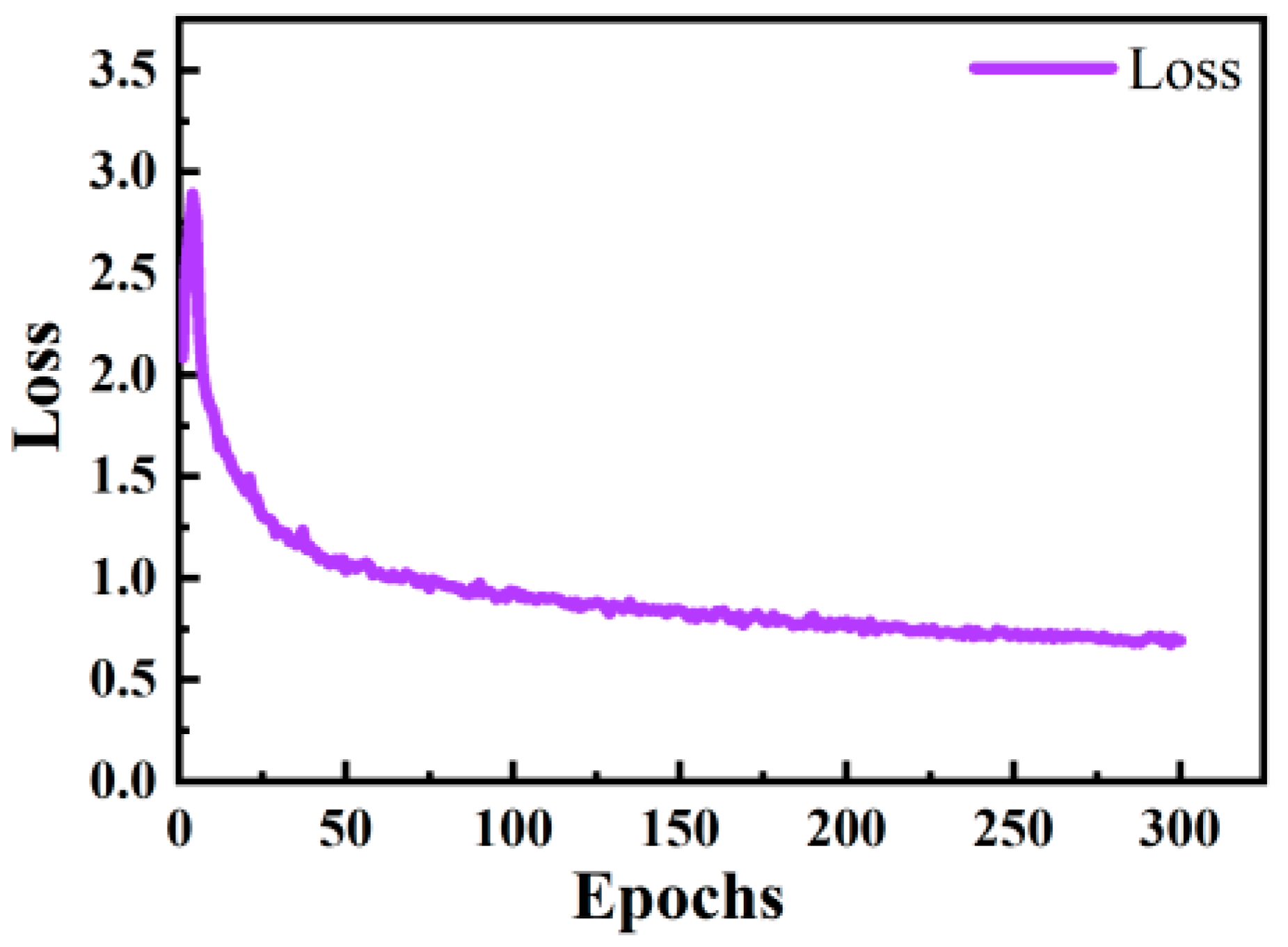
2.3.4. Training Process

When training the detection network model, the following parameters were set: the number of iterations was 300, the weight decay coefficient was 0.0005, the initial learning rate was 0.01, the learning rate momentum was 0.937, and the batch size was 16. As shown in Figure 9 and Figure 10, the model stopped training after 300 iterations. At this point, the loss had decreased to 0.69 and the [email protected]% had reached 87.4%.

2.4. DBSCAN Clustering Module

DBSCAN (Density-Based Spatial Clustering of Applications with Noise) is a clustering algorithm that focuses on the density of samples [28]. The core principle of DBSCAN is density-based classification, where samples within a certain density range are considered to belong to the same cluster. The clustering effect is achieved by classifying samples based on their density. To illustrate the DBSCAN process in detail, we will use the measurement data of 150 fish numbered 10 as an example.

2.4.1. Pre-Processing of Clustering Data

After processing with the improved CS-YOLOv8s identification algorithm, the coordinate positions and quantity information of the fish identified in each frame of the video data were obtained. The quantity of fish detected in each frame and their corresponding coordinate information were recorded. Subsequently, the two-dimensional coordinate data were converted from the normalized image coordinates to the actual coordinates in the real-world context.

$$\begin{array}{c}\mathrm{X}=(\mathrm{x}-\mathrm{n})\ast (2\mathrm{r}/\mathrm{h})\ast \mathrm{w}\\ \mathrm{Y}=(\mathrm{y}-\mathrm{n})\ast \left(2\mathrm{r}\right)\end{array}$$

(3)

where (X, Y) represent the point $p^{\prime }$ coordinates in Figure 11a, (x, y) represent the point p coordinate in Figure 11b, n was set to 1/2, r is the sonar range, which was 300 cm, h is the image height in pixels, and w is the image width in pixels.

To convert the two-dimensional coordinate data into three-dimensional coordinates, depth information calculated based on the time of the video data was added. The depth calculation formula can be expressed as follows:

$$\mathrm{d}=\mathrm{t}\ast \mathrm{v}$$

(4)

where d is the water depth, t is the frame-by-frame time of the video, and v is the descending motion speed of the sonar.

In Figure 12, the purple and blue boxes represent different water layers. The blue and green hollow circles denote the radius of clustering. Solid circles represent fish. The purple solid circle indicates the core object of a cluster, while the red solid circle represents the data of the same fish observed in different water layers. The summarized three-dimensional coordinate data were divided into 11 water layers, each with a depth interval of 40 cm. This spacing was determined using a trigonometric function based on the sonar beam opening angle and the scanned radius of the cage. The data were segmented into 11 water layers, with an overlap of 15 cm between adjacent layers, based on the body length and height of the fish used in the experiment. The overlap between water layers was intentional to account for the possibility that fish might move between layers during measurement. This overlap helped minimize the impact of repeated scanning data on the coordinates of fish after clustering, ensuring a more accurate representation of fish locations.

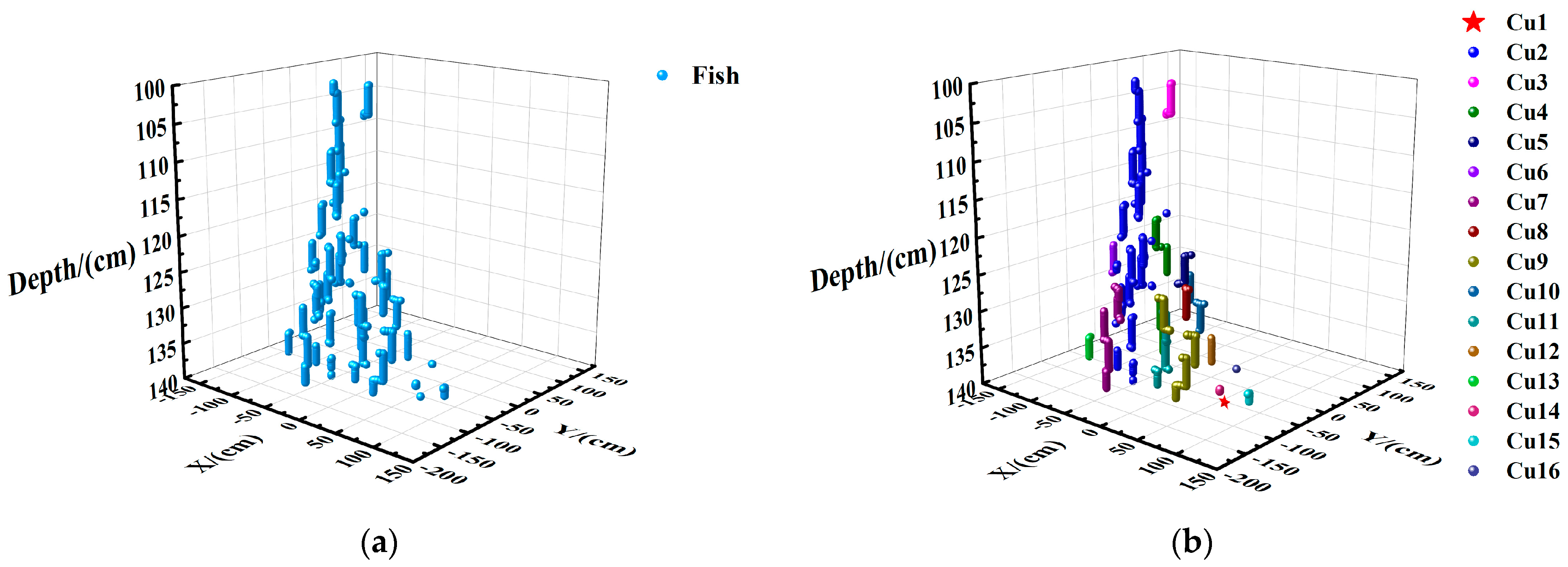
2.4.2. DBSCAN Clustering

The 3D data for each water layer were clustered using DBSCAN clustering analysis, with the following parameter settings: epsilon = 20.0, min_samples = 1. Considering the body length of the fish (approximately 24 cm) and their body height (approximately 12 cm), as well as the tendency for fish to school, the radius of clustering was set to 20.0 cm. This radius was chosen because fish typically do not stay very close to each other for extended periods. In this clustering setup, a hypersphere with a center at the coordinate of each fish and a radius of 20 cm was used. If additional coordinate points fell within this hypersphere, they were considered to belong to the same fish, since multiple fish are unlikely to be positioned very close to each other for long periods. Thus, the DBSCAN parameters were chosen to ensure that individual fish could be distinguished even if they were close together, reflecting the experimental conditions and the natural behavior of the fish.

Taking the data from the 100–140 cm water layer as an example, the spatial distribution of all coordinate points within this water layer is illustrated in Figure 13a. After traversing all points in the water layer, points that fell within the hypersphere with an epsilon radius of 20 cm were classified into the same cluster. This resulted in a total of 5384 coordinate points in this water layer. After applying DBSCAN clustering, these points were divided into 16 clusters, including noise clusters. The clusters were identified by different colors, as shown in Figure 13b.

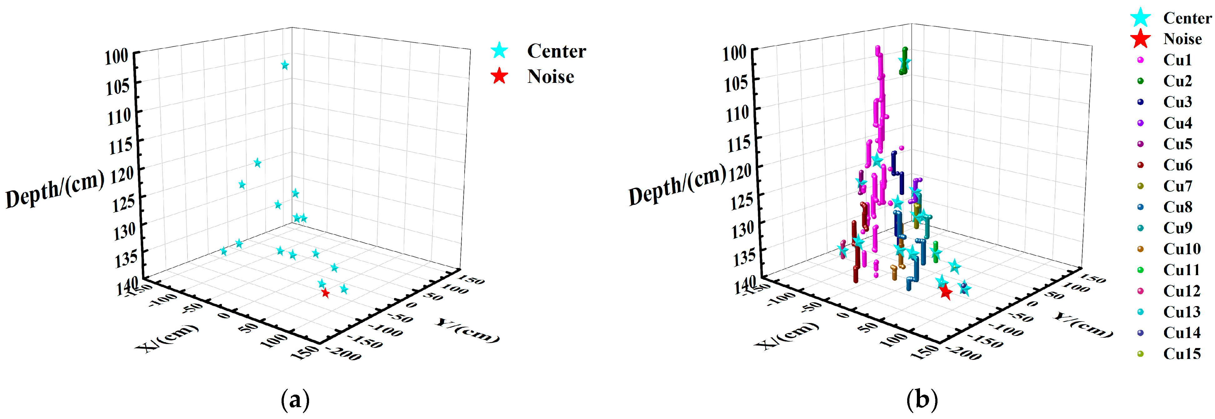
2.4.3. Reduction and Display of Noise Point

During clustering, attention should be focused on two types of data: core objects and noise points. Core objects are the coordinate points that meet the clustering parameters set (e.g., within the epsilon radius) and are considered the main components of a cluster. Core objects are crucial as they form the basis of the clusters and represent grouped fish. Noise points are coordinate points that do not meet the clustering parameters and are classified as noise during the clustering process. From a practical perspective, noise points indicate locations where there is only one fish within a certain range without interference from other fish. Each noise point represents a fish that should not be disregarded. In subsequent data processing, it is essential to comprehensively consider both core objects and noise points to ensure accurate fish count and distribution analysis.

As shown in Figure 14, the data of 5384 points in the 100–140 cm water layer were selected from the sonar images for experimental analysis. All data points of the water layer are shown in Figure 14a, and experimental results after clustering parameters (epsilon = 20.0, min_samples = 1) are displayed in Figure 14b. In Figure 14b, the red “★” (Cu1) represents the noise point identified by clustering, totaling one noise point. The remaining clusters, composed of core objects, are also shown, with a total of 15 clusters identified, excluding noise points. In the statistical process, clusters are counted as single fish. Noise points are counted individually as each represents an independent fish. The ”Noise” cluster, which consists solely of noise points, should not be counted as a fish. This method ensures that both core objects and noise points are accurately accounted for in the fish distribution analysis.

2.4.4. Reduction and Experiment Display of Center

To display clusters and centers more intuitively, the study used data from 5384 points in the 100–140 cm water layer, selected from the previous sonar images. The clustering parameters used were epsilon = 20.0 and min_samples = 1. After clustering, clusters representing coordinate points identified as the same fish were obtained. Given the difficulty in counting all coordinate points for spatial distribution analysis, each cluster was centralized to select a representative center point. This approach facilitated the study of fish distribution. Note that the “Noise” cluster, consisting solely of noise points, was not included in this centralization process and was counted point by point. The centers of each cluster were calculated, and their coordinates are provided in

Table 2. Coordinates of cluster centers in the 100–140 cm water layer.

Cluster Center	X/cm	Y/cm	Depth/cm
1	−35.4	2.0	22.8
2	16.2	16.3	8.8
3	−133.6	72.8	17.1
4	−157.0	42.1	17.2
5	−68.4	132.8	19.6
6	−107.9	106.8	22.9
7	−106.3	−2.6	18.8
8	−12.6	42.6	33.0
9	−38.8	99.6	34.0
10	−151.1	99.0	29.5
11	−86.9	84.3	29.5
12	37.1	−21.9	35.1
13	−69.4	104.5	36.3
14	−28.4	−113.4	38.8

and

Table 3. Coordinates of cluster noise point in the 100–140 cm water layer.

Noise	X/cm	Y/cm	Depth/cm
1	16.4	40.4	11.9

.

The calculated center coordinates and noise points of each cluster are displayed in Figure 15. In Figure 15a, the red “★” markers indicate noise points, while cyan “★” markers indicate the centers of each cluster. The color shading of the icons reflects the distance of coordinate points within each cluster along with the center of each cluster. The clustering effect is demonstrated to be effective.

2.4.5. Data Statistics of Water Layer

The quantity of fish in each water layer was determined by clustering the data for each water layer using the parameters epsilon = 20.0 and min_samples = 1. The results are summarized in

Table 4. Statistics of clustering results.

Water Layer/cm	Total Number of Coordinate Points/Piece	Number of Clusters (Including Noise Clusters)/Piece	Number of Noise Points/Piece	Number of Fish in This Layer/Piece
0~40	439	2	0	2
25~65	0	0	0	0
50~90	792	4	0	4
75~115	1794	5	0	5
100~140	5384	16	1	16
125~165	11,242	31	1	31
150~190	15,273	19	1	19
175~215	15,431	18	2	19
200~240	11,861	40	2	41
225~265	4432	26	0	26
250~290	253	2	0	2
Total	66,901	162	7	164

.

As shown in Table 4, clustering of the data from all water layers, totaling 66,901 points, resulted in 162 clusters, including 7 noise point clusters. The quantity of fish was estimated based on these clusters, with a total of 164 fish detected in the entire cage. Given that there were originally 150 fish in the target cage, the estimated quantity of 164 fish represents an error of 14 fish. This results in an accuracy rate of 90.7% and an error rate of 9.3%. Despite the slight overestimation, the high accuracy rate indicates that the clustering method was effective. Additionally, the method provided valuable information on the number of fish in each water layer, which is useful for analyzing the vertical distribution of fish in marine cages.

3. Results

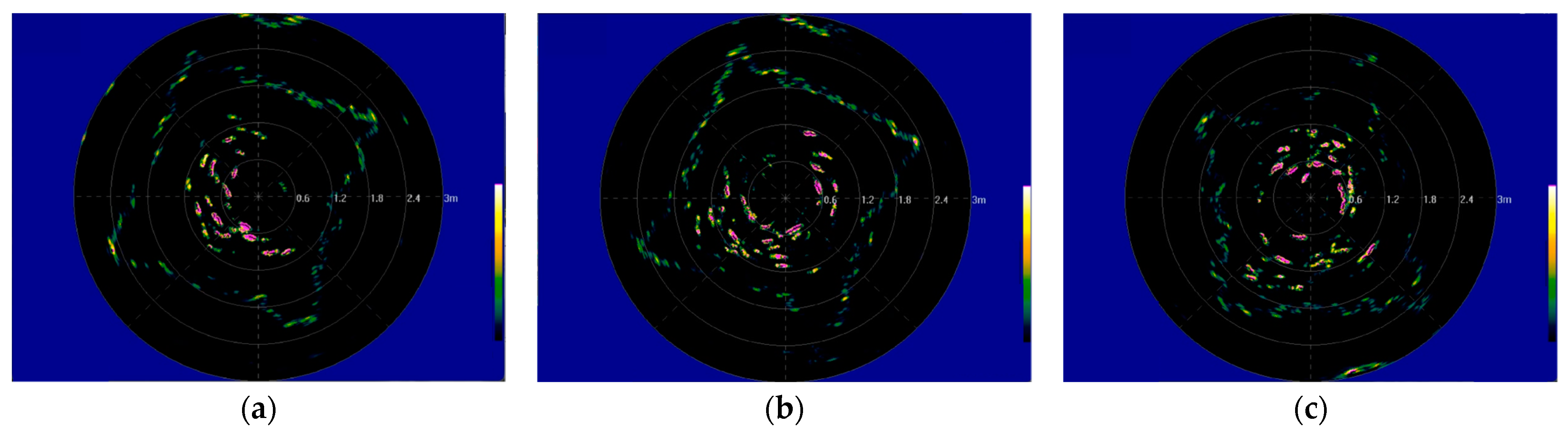
3.1. Result of Cage Data Acquisition

The sonar images depicting varying quantities of fish at a given moment are shown in Figure 16. The figure highlights several key observations:

Outer Contour: The outermost square in each image represents the contour of the netting within the cage.

Fish Contours: The fish-like shapes within the central portion of the netting indicate the presence of fish.

Additional Points: Smaller image points throughout the net garment represent fish at different locations and some noise points resulting from sea wave interference.

It is noted that the netting contours across the images are not identical, with missing segments visible in the middle and right images. These discrepancies were attributed to the changes of the net garment caused by the movement of sea waves.

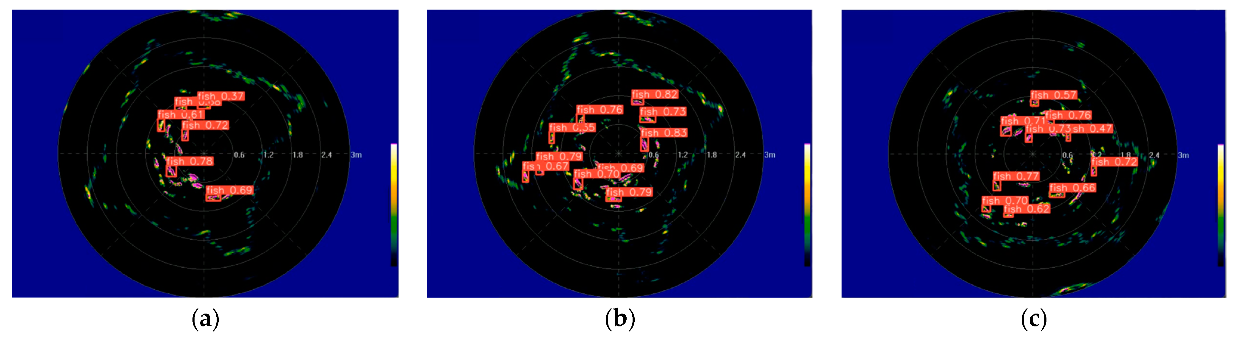
3.2. Data Processing

This paper concentrated on the analysis of the cage area to obtain detailed insights into the quantity and spatial distribution of fish across different water layers. The clustering analysis provided the quantity and coordinates of fish in each layer, allowing for an in-depth examination of their distribution patterns. This information was crucial for understanding fish behavior and enhancing feeding efficiency.

To ensure the fairness and effectiveness of model training, data processing was performed on each dataset of 200, 150, and 100 fish, respectively. The following evaluation metrics were used to assess the performance of the proposed method: accuracy, error rate, and number of errors. Sets of data from the 100 fish, 150 fish, and 200 fish datasets were selected (numbered 4, 10, and 16) as an example to illustrate the following in this section.

Number of Errors: This was calculated as the absolute value of the difference between the actual number of fish and the estimated number.

Error Rate: The error rate was determined as the percentage of the number of errors relative to the actual number of fish.

Average Error: This was computed as the mean of all error rates.

Average Precision: This was calculated as one minus the average error rate.

These metrics were used to comprehensively evaluate the accuracy and reliability of the proposed method.

The sonar image data, recorded as video data, were processed using the trained improved CS-YOLOv8s model for object identification (Figure 17). This model analyzed the sonar video data to extract information on the identified fish.

The image coordinates were converted into actual coordinate data using the ratio of image pixels to the actual cage size. Depth data, based on the sonar’s motion rate, were added to the coordinate information of the fish to form 3D coordinate data. The cage was then divided into 11 water layers, each with a depth interval of 40 cm. The coordinate data for fish identified in each water layer were obtained and clustered using the DBSCAN algorithm to estimate the fish coordinates within each layer.

The estimated distribution positions of the fish in the cage were summarized based on the estimated coordinate data. Additionally, a comparative analysis of fish distribution was conducted to evaluate the spatial arrangement and density of fish in different layers of the cage.

3.3. Result Analysis

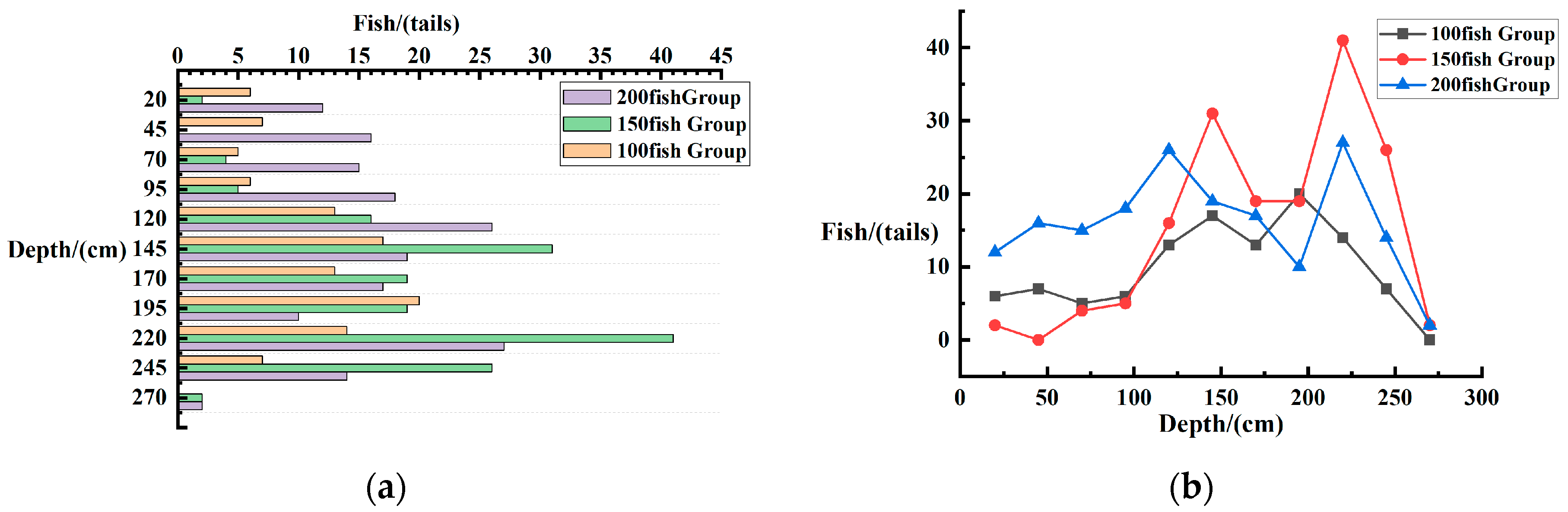
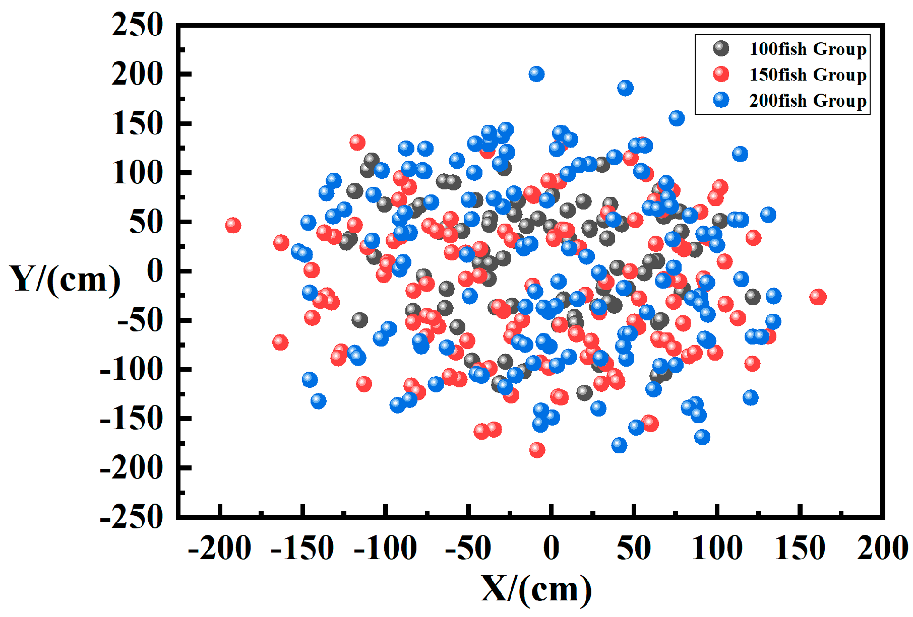
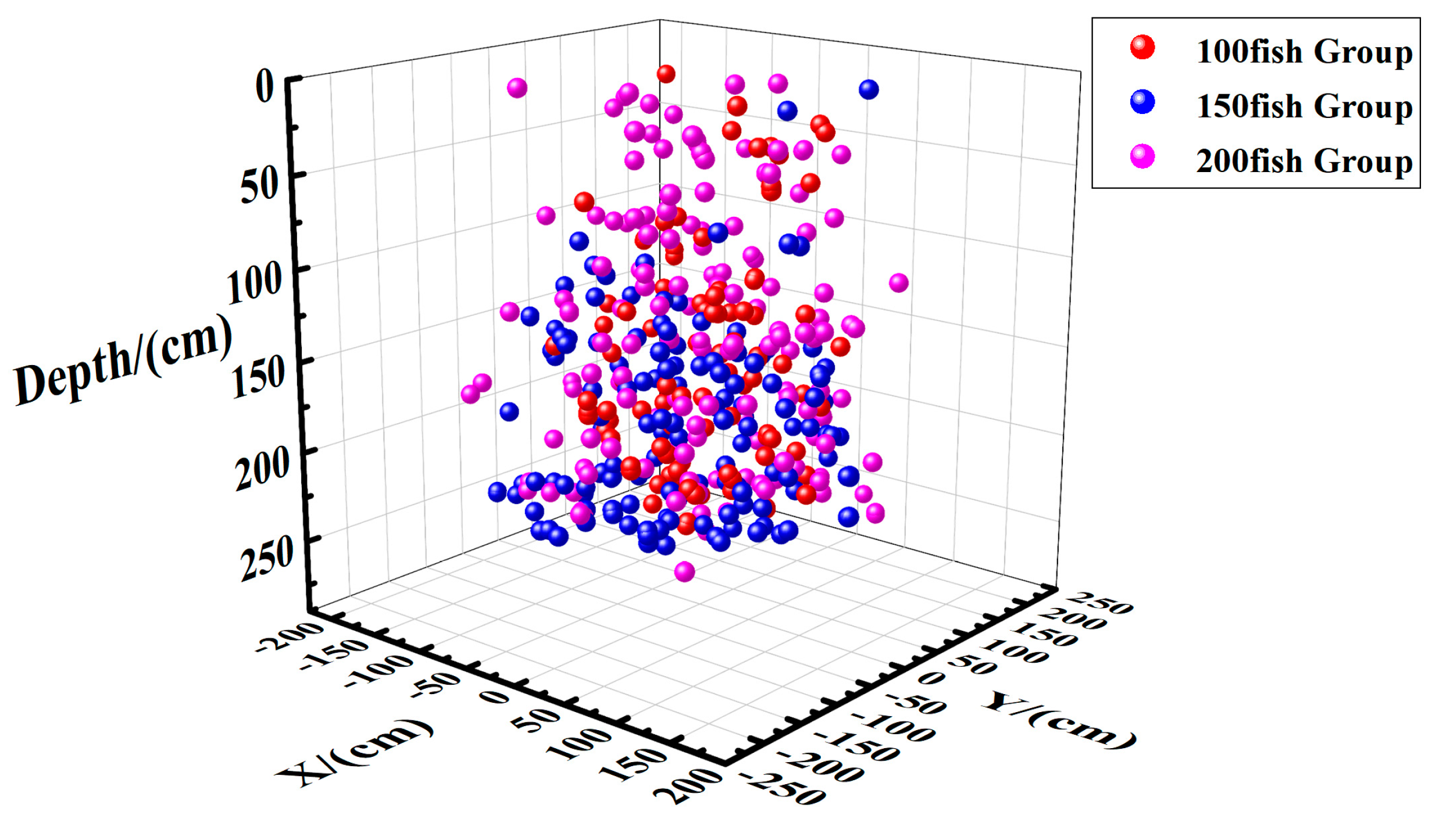
3.3.1. Effects of Quantity on Fish Distribution

Sets of data from the 100 fish, 150 fish, and 200 fish datasets were selected (numbered 4, 10, and 16) as an example to illustrate the following in this section. Based on the data on fish quantities in each layer obtained from clustering, the trend of fish numbers with depth was plotted, as shown in Figure 18. From Figure 18, it can be observed that the number of fish initially increased with depth before gradually decreasing. A significant concentration of fish was found within the depth range of 1.25 to 2.45 m, with the highest density at a depth of 2.25 m. This distribution pattern suggested that fish primarily preferred this depth range. Considering the impact of human factors [29,30], it was noted that the vertical distribution of fish might have been influenced by activities on the fishing rafts. Fish tended to seek refuge below 1.25 m in response to human presence, indicating behavioral adjustments to avoid disturbances.

Horizontal Spatial Distribution of Fish

According to the coordinates of fish in each layer obtained from clustering, the horizontal distribution maps of fish for different experimental groups were plotted, as shown in Figure 19. In Figure 19, the origin of the coordinates (0, 0) denotes the position of the sonar. It can be observed from Figure 19 that as the number of fish increased, the horizontal distribution range expanded from a radius of approximately 1 m to a radius of 1.5 m. Additionally, Figure 19a shows that a majority of fish were located around the sonar, suggesting that the moving sonar had some level of attraction for the fish. The summary of horizontal fish distribution across the three experimental groups is presented in Figure 20. The distribution was mainly concentrated within a radius of 1.5 m from the sonar, with a fairly even spread in all directions and only a few fish located near the edges. Considering the effects of fish domestication [31], the even distribution can be attributed to the variability in daily feeding positions, as fish were fed at various points in the cage. Consequently, no significant aggregation in a corner was observed, indicating a uniform horizontal distribution throughout the cage.

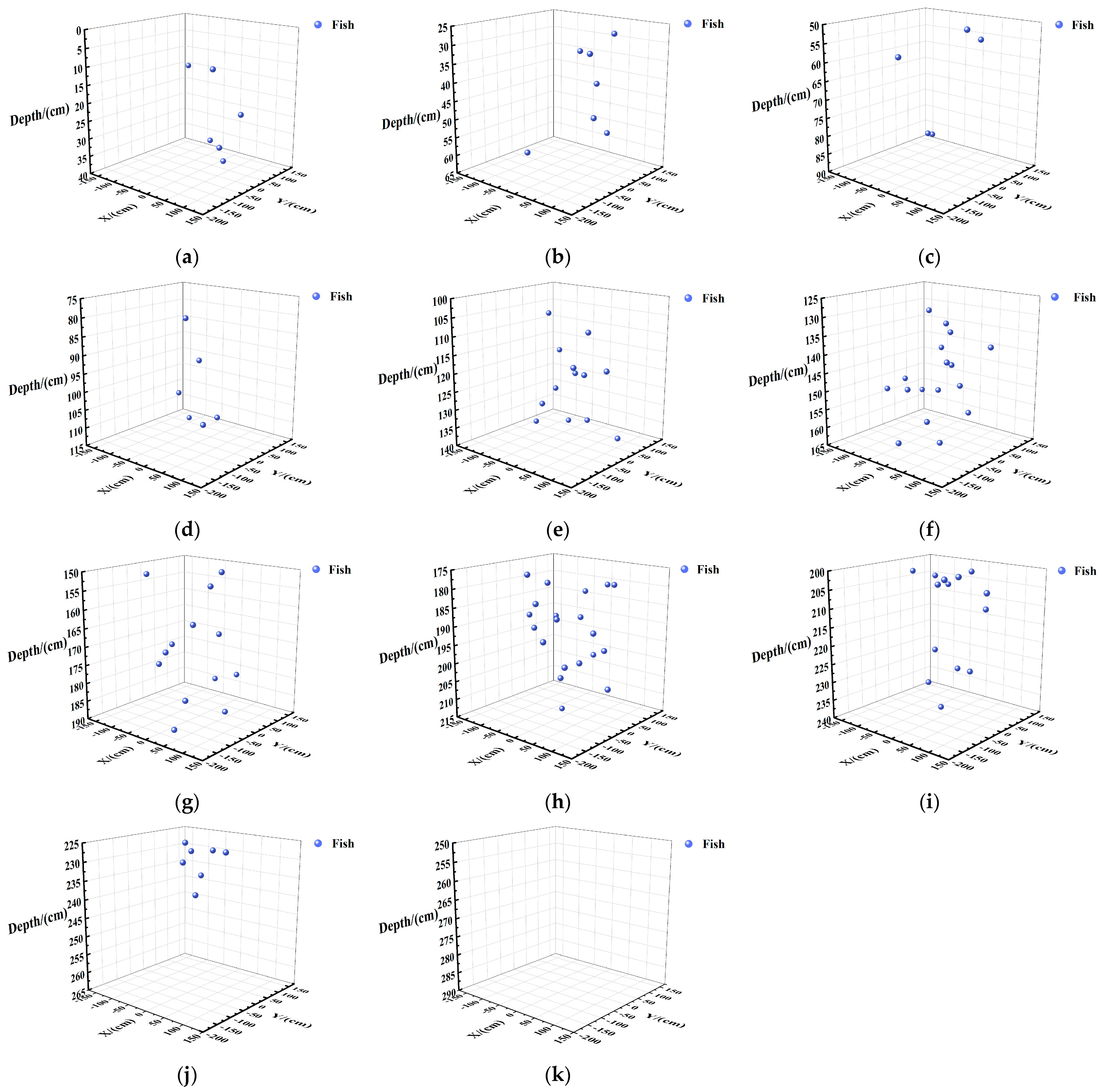
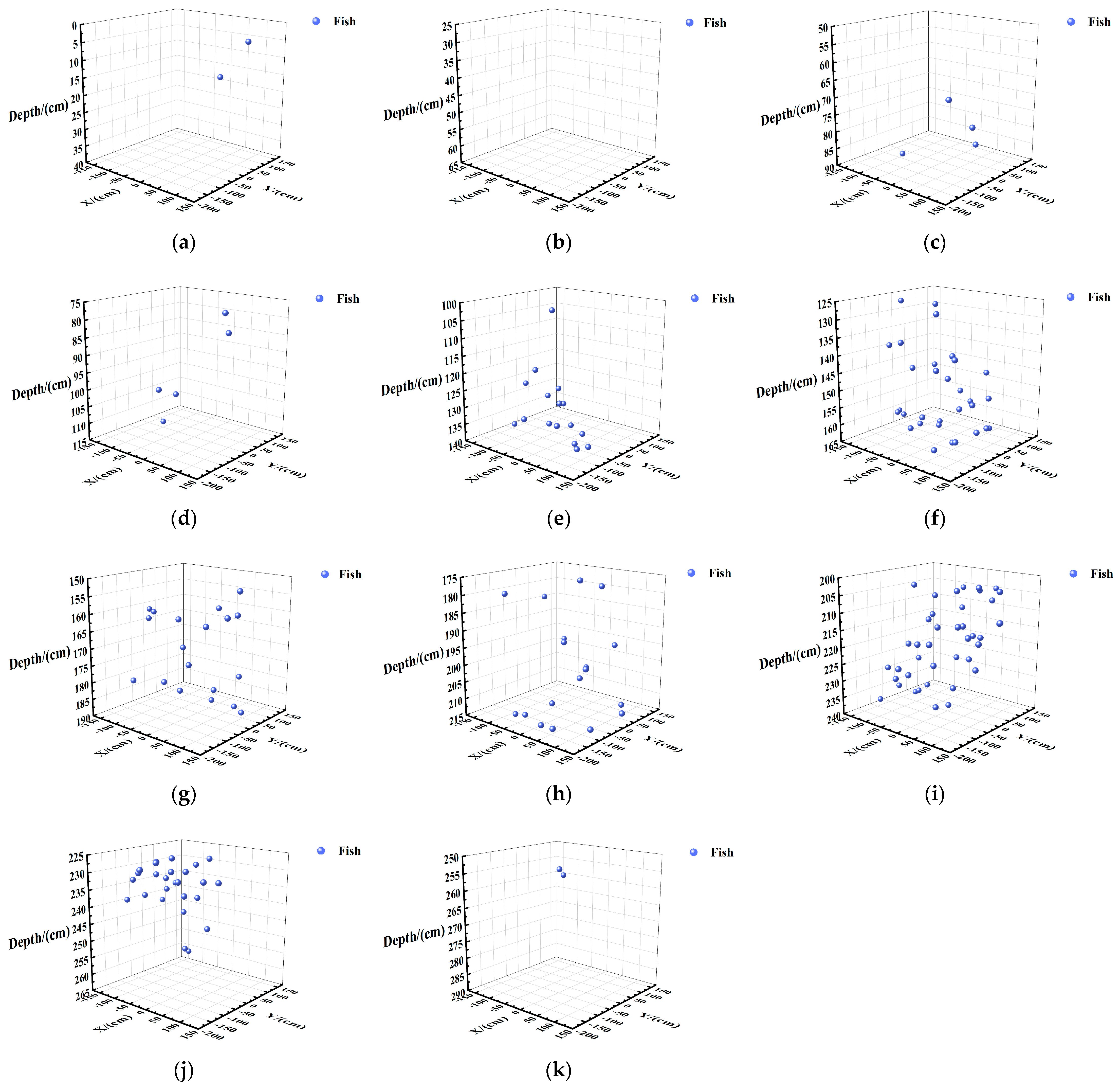
Vertical Spatial Distribution of Fish in Each Layer

To visually display the distribution of fish at different water layers, sets of data from the 100 fish, 150 fish, and 200 fish datasets were selected (numbered 4, 10, and 16) as an example to illustrate the following in this section.

This analysis utilized the 3D coordinates of fish obtained after clustering, resulting in 11 graphs that illustrate the predicted spatial distribution across the 11 water layers. These distributions are displayed in Figure 21, Figure 22 and Figure 23.

Figure 22a: Two fish were identified in this layer, located near the water surface with a depth of 15 cm and a horizontal distance of approximately 75 cm from the sonar.

Figure 22b: No fish were detected in this layer, indicating that either no fish were present or none were swimming through this water layer at the time.

Figure 22c: Four fish were found in this layer, distributed primarily 75 cm horizontally and 20 cm vertically from the sonar direction.

Figure 22f: Thirty-one fish were observed in this layer, with a concentration of approximately 100 cm horizontally from the sonar, mainly in the middle and lower parts of the water layer, and fewer in the upper part.

The figures demonstrate that the quantity of fish increased with depth up to a certain point and then decreased. The fish were mainly concentrated in the water depth range of 150 to 250 cm, with an even horizontal distribution and no extreme concentrations. The culture density was assessed as reasonable.

Vertical Spatial Distribution of Fish

Based on the 3D coordinates of fish in each layer obtained from clustering, the 3D spatial distribution maps of fish in the entire cage were plotted, as shown in Figure 24. The spatial distribution of fish for experimental groups with varying numbers of fish are described in the three panels of Figure 24. In these maps, the balls represent individual fish, with red, green, and blue circles indicating the projections of fish on the XOY, XOD (Depth), and YOD (Depth) axes, respectively. These projections illustrate the positional status of fish in three dimensions. From the projections on the XOD (Depth) and YOD (Depth) axes in Figure 24, it is evident that the number of fish increases with greater water depth. Additionally, the projection on the YOD (Depth) axis reveals that there are more fish in the positive direction of the Y-axis compared to the negative direction. This difference can be attributed to the effects of seawater flow within the marine cage, which causes fish to move downstream more frequently, resulting in a higher concentration of fish on one side of the cage.

The comparison of fish spatial distribution in experimental groups with different fish quantities are described in Figure 25. The 3D spatial distribution maps provide insights into the main activity ranges of the fish within the cage. As shown, the primary activity range of the fish spans from 1.5 m to 2.5 m in water depth and within a horizontal radius of 1.5 m, with no significant clustering in corners. As the number of fish increases, their distribution gradually extends from the bottom upwards. In conjunction with the analysis of fish distribution characteristics in culture cages as reported in the literature [32], the primary reasons for these observed distribution patterns can be summarized as follows: Long-term feeding in culture cages typically leads to a domestication effect, causing fish to aggregate around feeding positions. However, in the cages used in this study, which were relatively small, the domestication effect was not pronounced. Consequently, the fish were distributed more evenly throughout the cage rather than clustering around specific areas.

3.3.2. Effects of Sea Water Temperature on Fish Distribution

In this section, separate datasets of the same number of fish collected at different times have been selected as examples to illustrate the effects of sea water temperature on fish distribution. Temperature variations in seawater temperatures at three time points, morning, midday and evening, are useful for exploring the effects of temperature on fish distribution. Next, we will compare and analyze the data from the three time points of 8:00, 13:00, and 18:00, respectively. The sea water temperature was approximately 16, 19, and 18 degrees Celsius for the three time periods, respectively.

As shown in Figure 26, with the change of seawater temperature, some changes in fish distribution also occurred. As shown in Figure 26a, at 8:00, the distribution of fish was mainly concentrated in the 2 m water depth range. At 13:00, the distribution of fish gradually shifted to the 1 m water depth range as the temperature increased; finally, at 18:00, the distribution of fish returned to the 1.5 m water depth range. As shown in

Table 5. Distribution of fish in different datasets.

	Data Number	1	3	5	7	9	11	13	15	17
Water Layer/cm
0~40		3	4	6	3	5	5	5	12	5
25~65		6	8	7	5	4	7	3	16	10
50~90		2	13	9	7	13	8	9	15	19
75~115		5	16	12	11	18	13	14	18	25
100~140		12	14	11	12	22	20	31	26	30
125~165		14	11	18	22	24	25	23	19	21
150~190		16	10	13	22	21	28	14	17	22
175~215		13	8	10	20	24	17	16	10	20
200~240		10	3	4	23	20	10	35	27	26
225~265		3	1	3	15	5	7	26	18	20
250~290		2	0	0	4	2	3	7	2	7
Total		86	88	93	144	158	143	183	180	205

, data numbered 1, 7, and 13 are for 8:00; data numbered 3, 9, and 15 are for 13:00.; data numbered 5, 11, and 17 are for 18:00; data numbered 1, 3, and 5 are for 100 fish; data numbered 7, 9, and 11 are for 150 fish; and data numbered 13, 15, and 17 are for 200 fish. From 1, 7, and 13, it can be seen that at 8:00 the fish are mainly distributed at 2 m and the distribution expands to both ends as the number increases, with the peak of the number expanding to 1.25 m and 2.25 m when the number reaches 200 fish. From 3, 9, and 15, it can be seen that the distribution of the number of fish gradually expands towards the surface as the temperature of seawater increases, and the number of fish in the shallow water above 1 m gradually increases. From 5, 11, and 17, it can be seen that the number of fish in the shallow water areas decreased, but still remained higher than the number at 8:00 Among the three sets of data from 13, 15, and 17, the three changes in the distribution of 200 fish were closer to each other, with peaks in numbers mainly in the 1.25 m and 2.25 m areas.

In conjunction with the analysis of fish distribution characteristics in culture cages as reported in the literature [33,34,35], the primary reasons for these observed distribution patterns can be summarized as follows: The primary factors influencing the vertical distribution of fish are water temperature and dissolved oxygen levels. Variations in these factors affect how fish distribute themselves vertically within the water column. Specifically, fish tend to position themselves in layers where water temperature and dissolved oxygen are optimal for their survival and comfort. Considering that, at 8:00, the temperature is low (16 degrees Celsius) and the temperature of seawater will drop after overnight loss, so the fish will be distributed in the middle and lower layers of the cages, and under the influence of the low temperature the fish’s appetite and activity are not high; as the sun rises, the temperature of the seawater gradually rises, and at 13:00 (19 degrees Celsius), the fish tends to be in the middle and upper areas of the cages, and under the influence of the long-term rearing, the fish will tend to be in the upper-middle waters of the cages waiting for food; at 18:00, the seawater has some temperature and has not yet been lost after a day of sunshine, and the seawater temperature is higher although the temperature is close to that at 8:00 in the morning, so the distribution of the fish will show a small amount of folding back to the lower-middle waters.

It was observed that Trachinotus ovatus predominantly occupied depths above 1 m. This depth provided protection from the sun and offered suitable water temperatures. This observation aligns with the typical distribution characteristics of cultured Trachinotus ovatus and can inform future cultivation practices. Based on these findings, it is recommended to develop a more targeted and scientific approach to fish culture, such as setting feeding stations at approximately 1 m deep. This strategy would ensure optimal feeding conditions and enhance the efficiency of feed usage, contributing to better feed conversion rates and overall culture performance. Compared to direct surface feeding, placing feeding stations at a fixed depth is more efficient. This approach minimizes feed waste caused by waves, enhances feed conversion rates, improves culture efficiency, and reduces overall culture costs.

4. Discussion

The methods for monitoring fish include IoT-based fish monitoring systems [36], deep convolutional neural networks [37], deep learning [38], and species checklist data methods [39]. Due to the impossibility of conducting comparative experiments in the same environment, the instruments, equipment, and methods used in various methods are different. The comparison of different estimation and monitoring methods are shown in

Table 6. Comparison of different estimation and monitoring methods.

Methods	Equipment Usage	Monitoring Content	Advantage	Disadvantage
IoT-based fish monitoring system	A pH sensor, a temperature sensor, and some other equipment	pH level, the water temperature, dissolved oxygen level, and ammonia level	Monitoring various indicators of water quality can provide a healthy breeding environment for fish.	Lack of estimation of the number and distribution of fish populations in aquaculture water bodies makes it impossible to comprehensively consider water issues.
Deep convolutional neural networks	Electronic monitoring systems (EMSs)	The number of the fish, the types and body lengths of the fish	Automated, high precision	High computational burden
Deep learning	Sonar (oculusM750d)	Fish counting and tracking	Real-time data	Data limitation
Species checklist data method	Bottom trawl nets	Differences in fish assemblages	Large scale, diverse species	High demand for data and difficulty in data analysis
Our method	omnidirectional scanning sonar	Distribution of fish	Convenient, low implementation difficulty	The estimated range is small, lack of applicability to large sample data

.

As shown in Table 6, fish monitoring systems are often used to monitor the aquaculture environment, monitor the health of aquaculture water bodies, and adjust them in a timely manner to reduce fish losses. However, there is a lack of estimation of the amount of aquaculture in aquaculture water bodies, making it impossible to conduct comprehensive evaluations; two fish monitoring methods using neural networks are mainly used for estimating fish numbers. The trained models have high accuracy in estimating fish numbers, but their applicability is not high. A large amount of sample data is required to train the model to achieve the desired effect. The method of using species inventory data to estimate the spatial distribution of fish is mainly used for the overall distribution of fish diversity in large water areas and requires a large number of datasets for analysis. By comparison, the method proposed in this article is suitable for the spatial estimation of small-scale aquaculture and can accurately estimate the water depth and location of fish, making it easier for breeders to monitor the density and other conditions of aquaculture for management and adjustment of aquaculture plans.

5. Conclusions

In this study, data from Trachinotus ovatus aquaculture cages were acquired using omnidirectional scanning sonar. The distribution of cage fish was estimated using the proposed method, which presents innovative advantages over traditional and existing methods. Compared to traditional and existing methods, the approach proposed in this study was innovative in the identification and distribution estimation of fish. This innovation is highlighted in the following aspects:

(1)

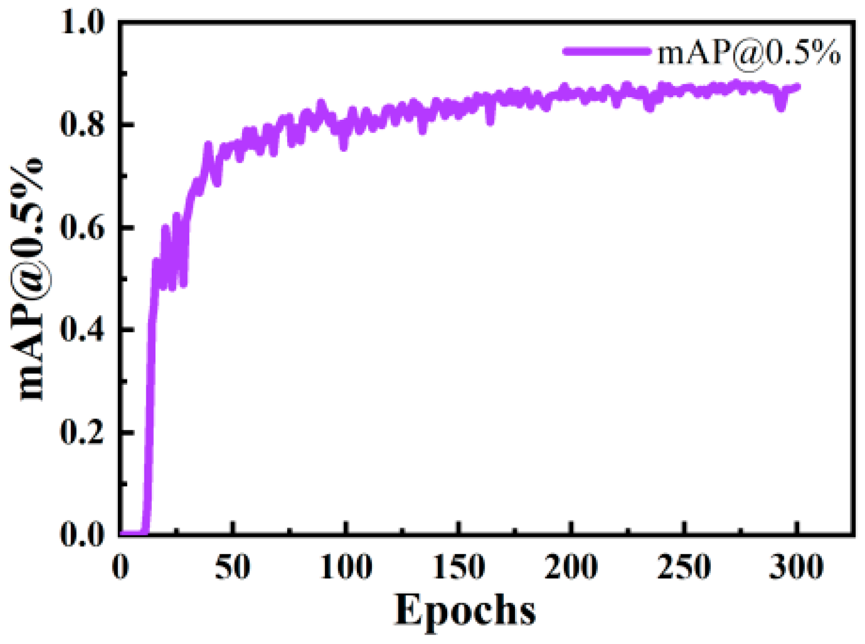
The fish sonar image object detection model was enhanced and trained by incorporating an attention mechanism into the YOLOv8s backbone network. This modification aimed to improve the model’s capability to detect small objects, making it more suitable for detecting fish in sonar images. Subsequently, ablation studies and model comparison experiments were conducted. The results demonstrated that the improved CS-YOLOv8s network achieved a [email protected] score that was 1.4% higher than that of the original YOLOv8s algorithm, as illustrated by the experimental results.

(2)

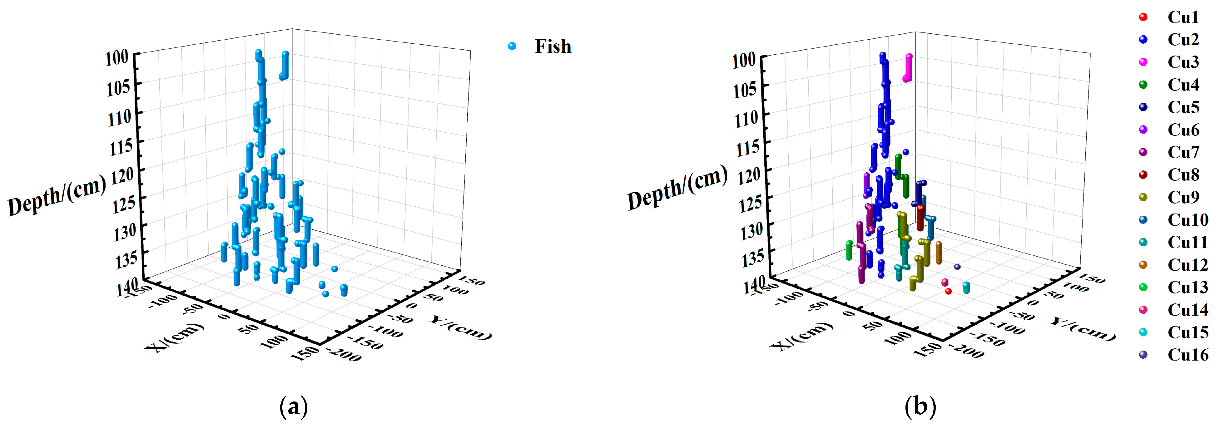
The quantity of fish was estimated layer by layer using the DBSCAN clustering algorithm, which provided the estimated positional coordinates of fish within each layer. This approach effectively addressed the issue of significant statistical errors associated with existing methods for tracking fish swimming, resulting in more accurate estimations.

An estimation method for the distribution of Trachinotus ovatus in marine cages was developed using omnidirectional scanning sonar and two advanced models. The approach involved placing the sonar at the center of the cage’s surface to conduct spiral descent scanning measurements. The improved YOLO model was employed to detect fish in the sonar images and extract their image coordinates. Subsequently, the cage was divided into water layers based on depth intervals. Clustering algorithms were used to estimate the actual coordinates of fish within each layer. By summarizing the coordinate data across all water layers, the overall distribution of fish in the cage was determined. Comparison experiments were performed on small cages, and sonar detection was conducted in groups according to the number of fish and the sea water temperature. The method provided distribution estimates that closely matched manual exploration results, demonstrating its effectiveness and suitability for practical applications, as evidenced by multiple experimental results.

However, this study is in the preliminary exploration stage and requires extensive experimentation to verify the accuracy and practicality of the method. Additionally, the fish distribution estimation method proposed in this study has certain limitations. Specifically, when fish quantities are large and dense, occlusion between fish can significantly affect the estimation results. Future research will focus on addressing these high-density occlusion issues to improve the method’s adaptability in estimating fish distribution under various cage aquaculture conditions.

References

1. Cheng, Z.X.; Hong, G.Q.; Li, Q.B.; Liu, S.H.; Wang, S.; Ma, Y. Seasonal dynamics of coastal pollution migration in open waters with intensive marine ranching. Mar. Environ. Res. 2023, 190, 106101. [Google Scholar] [CrossRef] [PubMed]
2. Liu, J.Y.; Gui, F.; Zhou, Q.; Cai, H.W.; Xu, K.D.; Zhao, S. Carbon Footprint of a Large Yellow Croaker Mariculture Models Based on Life-Cycle Assessment. Sustainability 2023, 15, 6658. [Google Scholar] [CrossRef]
3. Jeeva, J.C.; Ghosh, S.; Raju, S.S.; Megarajan, S.; Vipinkumar, V.P.; Edward, L.; Narayanakumar, R. Success of cage farming of marine finfishes in doubling farmers’ income: A techno-social impact analysis. Curr. Sci 2022, 123, 1031–1037. [Google Scholar] [CrossRef]
4. Banno, K.; Gao, S.; Anichini, M.; Stolz, C.; Tuene, S.A.; Gansel, L.C. Expanded vision for the spatial distribution of Atlantic salmon in sea cages. Aquaculture 2024, 588, 740879. [Google Scholar] [CrossRef]
5. Gamperl, A.K.; Zrini, Z.A.; Sandrelli, R.M. Atlantic salmon (Salmo salar) cage-site distribution, behavior, and physiology during a Newfoundland heat wave. Front. Physiol. 2021, 12, 719594. [Google Scholar] [CrossRef] [PubMed]
6. Johannesen, Á.; Patursson, Ø.; Kristmundsson, J.; Dam, S.P.; Muleid, M.; Klebert, P. Waves and currents decrease the available space in a salmon cage. PLoS ONE 2022, 17, e0263850. [Google Scholar] [CrossRef] [PubMed]
7. Ndashe, K.; Hang’ombe, B.M.; Changula, K.; Yabe, J.; Samutela, M.T.; Songe, M.M.; Kefi, A.S.; Chilufya, L.N.; Sukkel, M. An Assessment of the risk factors associated with disease outbreaks across tilapia farms in Central and Southern Zambia. Fishes 2023, 8, 49. [Google Scholar] [CrossRef]
8. Muñoz, L.; Aspillaga, E.; Palmer, M.; Saraiva, J.L.; Arechavala-Lopez, P. Acoustic telemetry: A tool to monitor fish swimming behavior in sea-cage aquaculture. Front. Mar. Sci. 2020, 7, 645. [Google Scholar] [CrossRef]
9. Proud, R.; Kloser, R.J.; Handegard, N.O.; Cox, M.J.; Brierley, A.S. Mapping the global prey-field: Combining acoustics, optics and net samples to reduce uncertainty in estimates of mesopelagic biomass. J. Acoust. Soc. Am. 2019, 146, 2898. [Google Scholar] [CrossRef]
10. Zhang, X.Y.; Gao, Y.H.; Ji, Y.Q.; Feng, A.W.; Zhao, S.J.; Wang, C.H. Compact multi-spectral-resolution Wynne-Offner imaging spectrometer with a long slit. Appl. Opt. 2024, 63, 1577–1582. [Google Scholar] [CrossRef]
11. Duan, Z.; Yuan, Y.; Lu, J.C.; Wang, J.L.; Li, Y.; Svanberg, S.; Zhao, G.Y. Underwater spatially, spectrally, and temporally resolved optical monitoring of aquatic fauna. Opt. Express 2020, 28, 2600–2610. [Google Scholar] [CrossRef] [PubMed]
12. Pagniello, C.M.L.S.; Butler, J.; Rosen, A.; Sherwood, A.; Roberts, P.L.D.; Parnell, P.E.; Jaffe, J.S.; Širović, A. An Optical Imaging System for Capturing Images in Low-Light Aquatic Habitats Using Only Ambient Light. Oceanography 2021, 34, 71–77. [Google Scholar] [CrossRef]
13. Yang, L.; Chen, Y.Y.; Shen, T.; Yu, H.H.; Li, D.L. A BlendMask-VoVNetV2 method for quantifying fish school feeding behavior in industrial aquaculture. Comput. Electron. Agric. 2023, 211, 108005. [Google Scholar] [CrossRef]
14. Helminen, J.; Dauphin, G.J.; Linnansaari, T. Length measurement accuracy of adaptive resolution imaging sonar and a predictive model to assess adult Atlantic salmon (Salmo salar) into two size categories with long-range data in a river. J. Fish Biol. 2020, 97, 1009–1026. [Google Scholar] [CrossRef]
15. Le, Z.Y. Exploration and suggestion on effective protection of offshore fishery resources based on acoustic technology. ChinaAquatic Prod. 2022, 5, 58–60. [Google Scholar]
16. Shen, W.; Peng, Z.F.; Zhang, J. Identification and counting of fish targets using adaptive resolution imaging sonar. J. Fish Biol. 2024, 104, 422–432. [Google Scholar] [CrossRef]
17. Helminen, J.; O’Sullivan, A.M.; Linnansaari, T. Measuring tailbeat frequencies of three fish species from adaptive resolution imaging sonar data. Trans. Am. Fish. Soc. 2021, 150, 627–636. [Google Scholar] [CrossRef]
18. Wei, Y.G.; Duan, Y.H.; An, D. Monitoring fish using imaging sonar: Capacity, challenges and future perspective. Fish Fish. 2022, 23, 1347–1370. [Google Scholar] [CrossRef]
19. Hobbs, D.; Bigot, M.; Smith, R.E.W. Rio doce acoustic surveys of fish biomass and aquatic habitat. Integr. Environ. Assess. Manag. 2020, 16, 615–621. [Google Scholar] [CrossRef]
20. Feng, Y.H.; Wei, Y.G.; Sun, S.; Liu, C.; An, D.; Wang, J. Fish abundance estimation from multi-beam sonar by improved MCNN. Aquat. Ecol. 2023, 57, 895–911. [Google Scholar] [CrossRef]
21. Stacy-Duffy, W.L.; Redman, R.A.; Roswell, C.R.; Peterson, S.D.; Czesny, S.J. Evaluation of fish spawning habitat at offshore reefs in southwest Lake Michigan using side-scan sonar and underwater video. Aquat. Conserv. Mar. Freshw. Ecosyst. 2024, 34, e4092. [Google Scholar] [CrossRef]
22. Jing, D.X.; Zhou, H.Y.; Han, J.; Zhang, J. Fish abundance estimation based on an imaging sonar. Appl. Acoust. 2019, 38, 705–711. [Google Scholar] [CrossRef]
23. Chevallay, M.; Du Dot, T.J.; Goulet, P.; Fonvieille, N.; Craig, C.; Picard, B.; Guinet, C. Spies of the deep: An animal-borne active sonar and bioluminescence tag to characterise mesopelagic prey size and behaviour in distinct oceanographic domains. Deep. Sea Res. Part I Oceanogr. Res. Pap. 2024, 203, 104214. [Google Scholar] [CrossRef]
24. Cui, Z.; Zhu, H.H.; Chen, C.; Liu, W.; Wang, Q.; Chai, Z.G. Study on Fish Resource Assessment Method Based on Imaging Sonar. In Proceedings of the 2022 3rd International Conference on Geology, Map** and Remote Sensing (ICGMRS), Zhoushan, China, 22–24 April 2022; IEEE: New York, NY, USA, 2022; pp. 327–331. [Google Scholar] [CrossRef]
25. Talaat, F.M.; Hanaa, Z.E. An improved fire detection approach based on YOLO-v8 for smart cities. Neural Comput. Appl. 2023, 35, 20939–20954. [Google Scholar] [CrossRef]
26. Li, Y.H.; Yao, T.; Pan, Y.W.; Mei, T. Contextual Transformer Networks for Visual Recognition. IEEE Trans. Pattern Anal. Mach. Intell. 2023, 45, 1489–1500. [Google Scholar] [CrossRef] [PubMed]
27. Jin, X.; Jiao, H.W.; Zhang, C.; Li, M.Y.; Zhao, B.; Liu, G.W.; Ji, J.T. Hydroponic lettuce defective leaves identification based on improved YOLOv5s. Front. Plant Sci. 2023, 14, 1242337. [Google Scholar] [CrossRef]
28. Yang, W.J.; Zhu, Z.Y.; Zhou, M.; Li, D.; Zhang, J.T.; Qin, M.Y.; Liu, B.L. Extraction of Tooth Cusps based on DBSCAN Density Clustering and Neighborhood Search Algorithm. Crit. Rev. Biomed. Eng. 2024, 52, 27–37. [Google Scholar] [CrossRef]
29. Cong, T.T.; Tong, C.F.; Zhao, C.J.; Chen, Z.T.; He, Z.F.; Liu, M.Y. Community composition and distribution characteristics of the fish assemblages in the rivers of Chongming Island in summer. Acta Ecol. Sin. 2021, 41, 2067–2076. [Google Scholar] [CrossRef]
30. Mennad, M.; Bachari, N.E.I.; Ferhani, K.; Chabet Dis, C.; Bennoui, A.; Neghli, L.; Ben Smail, S. Spatiotemporal Distribution of Small Pelagic Fish Schools in the Western Algerian Coast. Thalass. Int. J. Mar. Sci. 2023, 39, 923–930. [Google Scholar] [CrossRef]
31. Wu, Y.D.; Yu, X.K.; Suo, N.; Bai, H.Q.; Ke, Q.Z.; Chen, J.; Pan, Y.; Zheng, W.Q.; Xu, P. Thermal tolerance, safety margins and acclimation capacity assessments reveal the climate vulnerability of large yellow croaker aquaculture. Aquaculture 2022, 561, 738665. [Google Scholar] [CrossRef]
32. Rioja, R.A.; Palomar-Abesamis, N.; Juinio-Meñez, M.A. Correction to: Associated effects of shading on the behavior, growth, and survival of Stichopus cf. horrens juveniles. Aquac. Int. 2021, 30, 1087–1088. [Google Scholar] [CrossRef]
33. Li, Y.; Gao, C.X.; Chen, J.H.; Wang, Q.; Zhao, J. Spatial–temporal distribution characteristics of Harpadon nehereus in the Yangtze River Estuary and its relationship with environmental factors. Front. Mar. Sci. 2024, 11, 1340522. [Google Scholar] [CrossRef]
34. Kurbanov, Y.K.; Vinogradskaya, A.V. Distribution, Ecology and Size Composition of the White-Blotched Skate Bathyraja maculata (Arhynchobatidae) in the Northeastern Sea of Okhotsk during the Hydrological Summer. J. Ichthyol. 2023, 63, 1092–1101. [Google Scholar] [CrossRef]
35. Li, R.; Amenyogbe, E.; Lu, Y.; Jin, J.; Xie, R.; Huang, J. Effects of low-temperature stress on intestinal structure, enzyme activities and metabolomic analysis of juvenile golden pompano (Trachinotus ovatus). Front. Mar. Sci. 2023, 10, 1114120. [Google Scholar] [CrossRef]
36. Tamim, A.T.; Begum, H.; Shachcho, S.A.; Khan, M.M.; Yeboah-Akowuah, B.; Masud, M.; AI-Amri, J.F. Development of IoT Based Fish Monitoring System for Aquaculture. Intell. Autom. Soft Comput. 2022, 32, 56–71. [Google Scholar] [CrossRef]
37. Tseng, C.H.; Kuo, Y.F. Detecting and counting harvested fish and identifying fish types in electronic monitoring system videos using deep convolutional neural networks. ICES J. Mar. Sci. 2020, 77, 1367–1378. [Google Scholar] [CrossRef]
38. Xing, B.W.; Sun, M.; Liu, Z.C.; Guan, L.W.; Han, J.T.; Yan, C.X.; Han, C. Sonar Fish School Detection and Counting Method Based on Improved YOLOv8 and BoT-SORT. J. Mar. Sci. Eng. 2024, 12, 964. [Google Scholar] [CrossRef]
39. Zhang, Q.T.; Hu, G.K. Utilization of species checklist data in revealing the spatial distribution of fish diversity. J. Fish Biol. 2020, 97, 817–826. [Google Scholar] [CrossRef]
Figure 1. Satellite image map of the experimental site.
Jmse 12 01571 g001
Figure 2. Aerial view of the experimental site.
Jmse 12 01571 g002
Figure 3. Cage used in the experiment.
Jmse 12 01571 g003
Figure 4. Trachinotus ovatus used in the experiment. (a) Body length; (b) Body height.
Jmse 12 01571 g004
Figure 5. Working principle diagram of omnidirectional scanning sonar. (a) Schematic diagram of sonar scanning; (b) Work diagram.
Jmse 12 01571 g005
Figure 6. Omnidirectional scanning sonar.
Jmse 12 01571 g006
Figure 7. Sonar Assembly.
Jmse 12 01571 g007
Figure 8. Side view of the sea cage. The sonar in the yellow box is located on the center axis of the net cage, and the yellow dotted lines shows the range covered by the sonar.
Jmse 12 01571 g008
Figure 9. Training process (Loss).
Jmse 12 01571 g009
Figure 10. Training process ([email protected]%).
Jmse 12 01571 g010
Figure 11. Coordinate transformation. (a) A coordinate system with sonar as the origin; (b) A coordinate system with the top left corner as the origin.
Jmse 12 01571 g011
Figure 12. Water layer division.
Jmse 12 01571 g012
Figure 13. Clustering in the 100–140 cm water layer. (a) Fish distribution; (b) Cluster effect diagram.
Jmse 12 01571 g013
Figure 14. Water layer data and the data after clustering. (a) Fish distribution map before clustering; (b) Cluster diagram of noisy points.
Jmse 12 01571 g014
Figure 15. Center and noise point of core object. (a) Distribution map of center point and noise point; (b) Centralization rendering.
Jmse 12 01571 g015
Figure 16. Sonar images of different numbers of fish. (a) 100 fish; (b) 150 fish; (c) 200 fish.
Jmse 12 01571 g016
Figure 17. Fish for object identification. (a) 100 fish; (b) 150 fish; (c) 200 fish.
Jmse 12 01571 g017
Figure 18. Trend of number of fish with depth. (a) Comparison bar chart of depth distribution; (b) Comparison line chart of fish depth distribution.
Jmse 12 01571 g018
Figure 19. Horizontal distribution maps of fish. (a) Horizontal distribution of 100 fish; (b) Horizontal distribution of 150 fish; (c) Horizontal distribution of 200 fish.
Jmse 12 01571 g019
Figure 20. Horizontal distribution comparison chart of fish.
Jmse 12 01571 g020
Figure 21. Spatial distribution maps of 100 Fish in each water layer. (a) Water layer: 0–40 cm; (b) Water layer: 25–65 cm; (c) Water layer: 50–90 cm; (d) Water layer: 75–115 cm; (e) Water layer: 100–140 cm; (f) Water layer: 125–165 cm; (g) Water layer: 150–190 cm; (h) Water layer: 175–215 cm; (i) Water layer: 200–240 cm; (j) Water layer: 225–265 cm; (k) Water layer: 250–290 cm.
Jmse 12 01571 g021
Figure 22. Spatial distribution maps of 150 Fish in each water layer. (a) Water layer: 0–40 cm; (b) Water layer: 25–65 cm; (c) Water layer: 50–90 cm; (d) Water layer: 75–115 cm; (e) Water layer: 100–140 cm; (f) Water layer: 125–165 cm; (g) Water layer: 150–190 cm; (h) Water layer: 175–215 cm; (i) Water layer: 200–240 cm; (j) Water layer: 225–265 cm; (k) Water layer: 250–290 cm.
Jmse 12 01571 g022
Figure 23. Spatial distribution maps of 200 fish in each water layer. (a) Water layer: 0–40 cm; (b) Water layer: 25–65 cm; (c) Water layer: 50–90 cm; (d) Water layer: 75–115 cm; (e) Water layer: 100–140 cm; (f) Water layer: 125–165 cm; (g) Water layer: 150–190 cm; (h) Water layer: 175–215 cm; (i) Water layer: 200–240 cm; (j) Water layer: 225–265 cm; (k) Water layer: 250–290 cm.
Jmse 12 01571 g023
Figure 24. 3D spatial distribution maps of cage fish. (a) Spatial distribution of 100 fish group; (b) Spatial distribution of 150 fish group; (c) Spatial distribution of 200 fish group.
Jmse 12 01571 g024
Figure 25. Spatial distribution comparison chart of fish.
Jmse 12 01571 g025
Figure 26. Distribution of fish at different temperatures. (a) Distribution of 100 fish; (b) Distribution of 150 fish; (c) Distribution of 200 fish.
Jmse 12 01571 g026