Numerical Investigation of the Hydrodynamic Characteristics of a Novel Bucket-Shaped Permeable Breakwater Using OpenFOAM

Abstract

To align with contemporary concepts of low-carbon and environmental protection, a new type of bucket-shaped permeable breakwater, based on the prototype of the bucket-based breakwater in Xuwei Port Area, Lianyungang, Jiangsu Province, China, was proposed. A three-dimensional numerical wave flume was constructed using the OpenFOAM platform and DXFlow (an open-source computational fluid dynamics toolbox based on OpenFOAM). The effectiveness of this numerical wave flume was validated through temporal and spatial verification, wave generation validation, and model testing. The study investigated the effects of bucket porosity, opening shapes, number of openings, and the positioning of these openings on the wave-dissipating performance under regular wave conditions. It analyzed the force characteristics near the openings. The results showed that within the relative wavelength range of L/D between 6.7 and 12.7, relative wave height H/d between 0.175 and 0.275, changes in wavelength had a limited impact on the wave-dissipating performance of the bucket-shaped permeable breakwater. The wave-dissipating performance was primarily related to the porosity, with the optimal overall wave-dissipating performance occurring at a bucket porosity of 12%. The shape and number of openings had a minimal relationship with performance. Additionally, the connecting walls of this type of breakwater experienced the most significant wave impact, suggesting that these areas should be reinforced in practical engineering applications.

1. Introduction

Breakwaters are among the most common structures in nearshore areas and play a crucial role in coastal protection and maintaining stable harbor conditions. Compared to traditional breakwaters, permeable breakwaters offer advantages such as reducing wave forces, minimizing wave reflection, allowing seawater and marine life to pass through, and having lower construction and maintenance costs. As a result, they hold significant potential for a wide range of applications.

Jarlan [1] first proposed the concept of perforations in the front wall of a submerged box breakwater and discovered that such structures could increase wave energy dissipation and reduce wave reflection. Subsequently, the concept inspired many researchers, who began employing various research methods to analyze the hydrodynamic characteristics of perforated breakwaters. These studies primarily encompass theoretical research, model experiments, and numerical simulations. Tanimoto and Yoshimoto [2] conducted theoretical and experimental research on the reflection characteristics of partially perforated breakwaters. In the same year, Wu [3] explored the effects of parameters such as relative chamber width, perforation ratio, perforation shape, and crest elevation of the wave-dissipating chamber on the hydrodynamic performance of perforated breakwaters. Fugazza and Natale [4] analyzed and proposed a calculation formula for wave forces on perforated breakwaters based on model experiments. Cox et al. [5] investigated the relationship between the reflection coefficient of single-layer and double-layer perforated panels and the relative width of the wave-dissipating chamber through model experiments. In the same year, based on model experiments, Bergmann and Oumeraci [6] analyzed the variation in point pressures at the same height of perforated caissons and perforated panels under the same still-water conditions through model experiments. They used experimental data to refine Goda’s formula. Neelamani and Vedagiri [7] investigated the wave propagation, reflection, and energy dissipation characteristics of partially submerged double vertical breakwaters under different wave climates and structural forms. Rao et al. [8] analyzed the effects of wave steepness, relative water depth, and inclined plate angles on wave propagation through model experiments. Takahashi et al. [9] conducted numerical simulations using the VOF method to study the interaction between waves and local perforated breakwaters. They analyzed the structure’s reflection coefficient and provided information about the flow field near the perforated breakwater. Wu et al. [10] developed a highly nonlinear numerical model for solving the interaction between waves and large perforated wave-dissipating structures. They also presented a method to calculate the wave pressure on the perforated panel. Wang et al. [11] used the boundary element method to analyze a double-pier permeable breakwater’s transmission and reflection coefficients. Numerical simulations offer greater flexibility and control than model experiments, with lower research costs. However, they rely heavily on the model’s accuracy and input data’s reliability, leading to a certain degree of error. Often, combining both approaches yields more accurate and reliable results. For instance, Gui et al. [12] investigated the hydrodynamic characteristics of perforated breakwaters through a combination of model experiments and numerical simulations, finding that a perforation rate of 4% yielded the lowest transmission coefficient for vertical pile-mounted perforated breakwaters. Yin et al. [13] proposed an inclined perforation slot breakwater scheme and studied its hydrodynamic characteristics in regular wave conditions using a combined approach of numerical simulations and physical model experiments.

In recent years, researchers have not only been committed to enhancing the accuracy of numerical simulations of wave interactions with perforated breakwaters [14,15] but have also explored various innovations based on perforated breakwaters [16,17,18,19,20]. With the widespread application of perforated breakwaters in practical engineering, the focus of scholars has gradually shifted towards “how to improve and optimize the structures.” Just as Tagliafierro et al. [21] took the example of a low-reflection sunken box constructed in a port in Spain, they conducted numerical simulation studies on sunken boxes with different chamber configurations and efficiency under varying sea conditions.

In response to the soft soil foundation conditions of silty coastlines in certain Chinese port areas, Chinese scholars have proposed a solution based on bucket-based structures, which was first successfully implemented in the Xuwei Port area of Lianyungang, Jiangsu Province (Figure 1). This bucket-based structure consists of a giant elliptical lower foundation bucket and two upper buckets of equal diameter connected by walls. The lower bucket is divided into multiple compartments but is open at the bottom, allowing it to embed into the silty soil foundation through negative pressure fully. The two upper buckets can be used either for wave blocking or soil retention. When the upper buckets are used for wave blocking, the structure functions as a bucket-shaped breakwater; when used for soil retention, it serves as a revetment or wharf. Research has shown that this structure has significant potential for application in areas with thick silt layers and highly compressible soils [22]. It also demonstrates excellent performance regarding construction efficiency and material costs [23]. The application of this new type of bucket foundation structure is gradually expanding and has been promoted domestically and internationally across various regions and fields. It has also been incorporated into the Ministry of Transport’s industry standard, “Design and Construction Specification for Bucket-base Structures of Port and Waterway Engineering JYS/T 167-16-2020” [24]. However, current research primarily focuses on structural stability [25,26,27], while studies on optimizing the hydrodynamic properties of the bucket structure remain relatively limited.

Taking into account the benefits of permeable breakwaters, such as improved water permeability, reduced wave forces, and minimized wave reflection, this paper uses the upper bucket section of the bucket-based breakwater in the Xuwei Port area of Lianyungang, Jiangsu Province, as a prototype. A bucket-shaped permeable breakwater is proposed based on the design principles of perforated caisson breakwaters (Figure 2). A three-dimensional numerical wave flume was established using the OpenFOAM platform and the open-source computational fluid dynamics toolbox DXFlow [28], developed by the research team. After multiple validations, including time, space, theoretical solutions, and model tests, the reliability of the numerical wave flume was confirmed. Subsequently, under regular wave conditions, this paper studied the impact of porosity, opening shape, number, and position on the wave dissipation performance of the bucket-shaped permeable breakwater. It analyzed the mechanical characteristics near the openings on the bucket walls. The aim is to provide a valuable reference for practical engineering applications.

2. Numerical Model Establishment

2.1. Governing Equations and Boundary Conditions

The Reynolds-averaged Navier–Stokes equations, consisting of the continuity and momentum equations, are used for incompressible viscous fluids [29,30]. Equations (1) and (2) show the mass conservation and momentum conservation equations. The Volume of Fluid (VOF) method determines the proportion of gas and liquid in the grid, and Equation (3) shows the VOF control equation [31]. Equation (4) gives the density $\rho$ and dynamic viscosity $\mu$ of the mixed fluid.

$$\nabla \cdot u=0$$

(1)

$${\displaystyle \frac{\partial \rho u}{\partial t}}+\nabla \cdot (\rho uu)-\nabla \cdot ((\mu +{\mu }_{tur})\nabla u)=C\kappa \nabla \alpha -gX\nabla \rho -\nabla P_{\rho gh}$$

(2)

$${\displaystyle \frac{\partial \alpha }{\partial t}}+\nabla \cdot (\alpha u)+\nabla \cdot [\alpha (1-\alpha )U_r]=0$$

(3)

where u is the fluid velocity vector; $\alpha$ is the fraction of the volume of fluid in the grid cell to the total volume of the grid cell. If at a certain moment the grid cell is completely filled with fluid, then α = 1, indicating a fluid cell; if at a certain moment the grid cell is completely filled with air, then α = 0, indicating an empty cell; if at a certain moment the grid cell contains both fluid and air, then 0 < α < 1, indicating a partially fluid cell. The fluid volume of the computational grid cell is determined based on the volume fraction α of the fluid in the neighboring grids and the fluid velocity at the boundaries of the grid cell, comprehensively considering the volume fraction α of the fluid in the neighboring grid cells to determine the position and shape of the free surface; t is the time; ${\mu }_{tur}$ is the dynamic turbulent viscosity; ρ and μ are the average density and dynamic viscosity of the two-phase flow, respectively, calculated as follows:

$$\left\{\begin{array}{l}\rho =\alpha {\rho }_1+(1-\alpha ){\rho }_2\\ \mu =\alpha {\mu }_1+(1-\alpha ){\mu }_2\end{array}\right.$$

(4)

In Equation (2), Cκ∇α represents the surface tension term, where C is the surface tension coefficient, and κ is the curvature of the interface. g is the acceleration of gravity; X is the position vector; ${\rho }_1$ is the density of water; ${\rho }_2$ is the density of air; ${\mu }_1$ is the dynamic viscosity of water; ${\mu }_2$ is the dynamic viscosity of air; $P_{\rho gh}$represents the pseudodynamic pressure:

$$P_{\rho gh}=P-\rho g\cdot X$$

(5)

where $P_{\rho gh}$has no physical meaning but is used to apply a convenient numerical technique. Equation (5) represents the dynamic pressure only if the free surface is located at Z = 0. The third term on the left side of Equation (3) is the artificial compression term, which is only effective at the free surface. $U_r$is the artificial compressive velocity [32,33]:

$$U_r=c_a\left|u\right|$$

(6)

where u is fluid velocity; $c_a$ is a factor with a default value of 1.0, and this value can be specified by users to enhance ($c_a$ > 1.0) or eliminate ($c_a=$ 0) the compression of the interface.

Additionally, due to the three-dimensional symmetric nature of this experimental model and to optimize computational resource allocation and improve efficiency, the front wall of the numerical wave flume is set as a symmetric boundary condition. The flow fields on both sides of this boundary are symmetric and mirror each other. The back wall, bottom, and walls of the structure in the flume employ a no-slip condition. When fixing the boundary, the velocity field at the boundary satisfies the no-slip need, as shown in Equation (7), and the pressure field on the wall satisfies the requirement of zero pressure gradient along the average direction, as shown in Equation (8).

$$U{|}_{wall}=0$$

(7)

$${\displaystyle \frac{\partial P}{\partial n}}=0$$

(8)

2.2. Wave Generation and Wave Absorption Methods

To simulate laboratory wave generation, this study employs the dynamic boundary wave generation method. According to linear theory, the relationship between the wave height and the push board stroke for regular waves can be expressed as:

$$H_s={\displaystyle \frac{H}{S}}={\displaystyle \frac{4{\sinh }^2(kd)}{2kd+\sinh 2kd}}$$

(9)

where $H_s$ is the transfer function, H is the wave height, S is the stroke of the wave generator paddle, k is the wave number, and d is the water depth. If the free surface of the target wave is:

$$\eta (x,t)={\displaystyle \frac{H}{2}}\cos (kx-\omega t)$$

(10)

The motion and velocity of the paddle (x = 0) can be expressed as:

$$X(t)={\displaystyle \frac{S}{2}}\sin (\omega t)$$

(11)

$$U(t)={\displaystyle \frac{S}{2}}\omega \cos (\omega t)$$

(12)

where t is the simulation time, and ω is the angular frequency.

The principle of damping wave dissipation involves adding a damping term to the momentum equation to achieve momentum attenuation in the numerical wave flume damping section, thereby eliminating reflected waves at the boundaries. This method was initially proposed by Larsen [34], where the expression for the momentum damping source term is:

$$S^{*}=\rho u\chi$$

(13)

$$\chi =\left\{\begin{array}{l}{\chi }_1\cdot {\displaystyle \frac{x-x_0}{L_s}},(x>x_0)\hfill \\ 0,\hspace{1em}\hspace{1em}\hspace{1em} (x\le x_0)\hfill \end{array}\right.$$

(14)

where $\rho$ is density, $u$ is fluid velocity, $\chi$ is the attenuation function, ${\chi }_1$ is the attenuation coefficient, $x$ is the horizontal coordinate in the Cartesian coordinate system, $x_0$ is the horizontal coordinate of the starting point of the damping wave dissipation zone, and $L_s$ is the length of the damping zone. The length of the damping zone should be 1 to 2 times the wavelength; therefore, the attenuation coefficient in this paper is set to 5.

2.3. Wave Dissipation Characteristic Coefficient

The reflection coefficient K_r, transmission coefficient K_t, and dissipation coefficient K_d are essential indicators that reflect the wave dissipation characteristics of the breakwater. Equations (15)–(17), respectively, show the calculation formulas [35]:

$$K_r={\displaystyle \frac{H_r}{H_i}}$$

(15)

$$K_t={\displaystyle \frac{H_t}{H_i}}$$

(16)

$$K_d=1-K_t^2-K_r^2$$

(17)

where $H_r$ is the reflected wave height, $H_i$ is the incident wave height, and $H_t$ is the transmitted wave height.

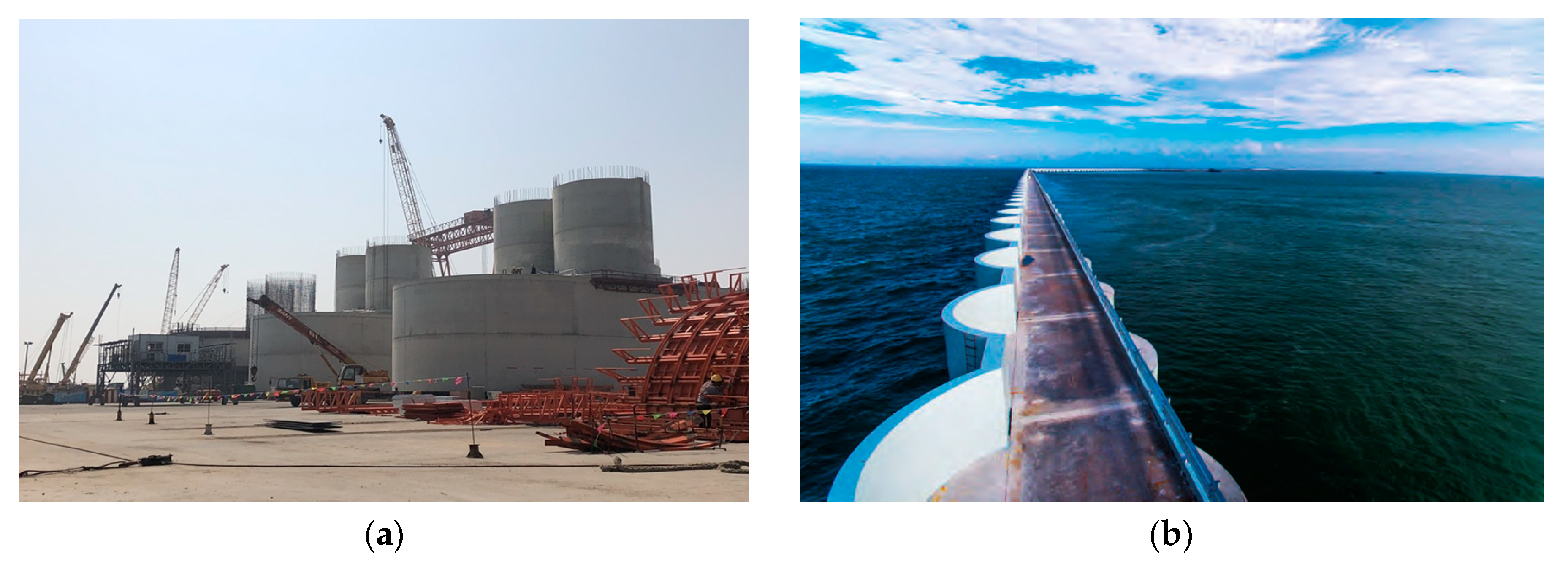
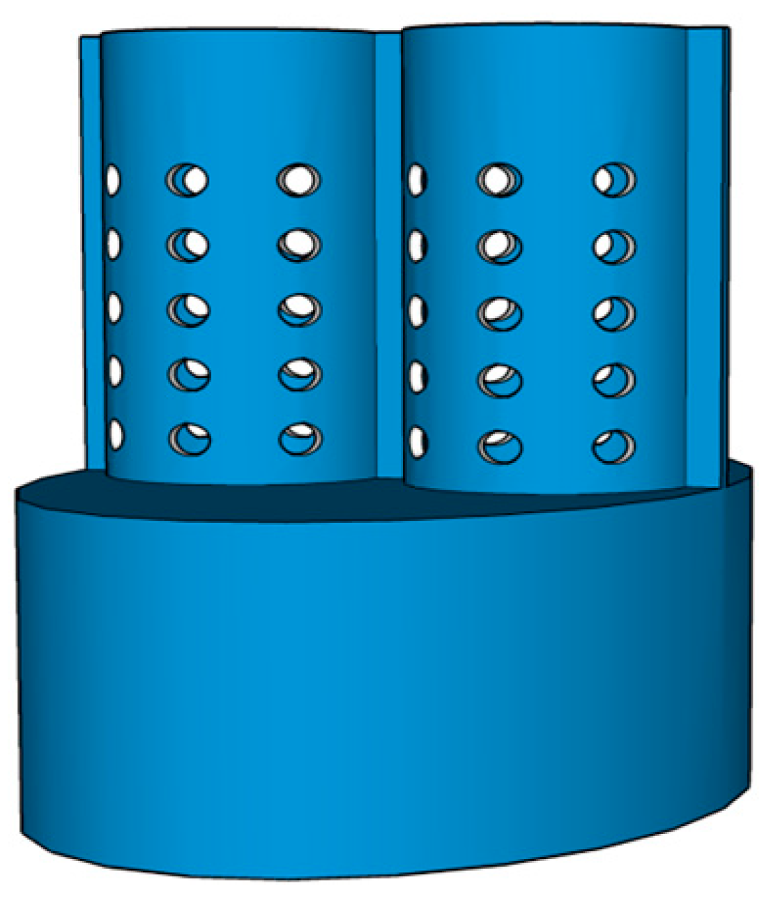
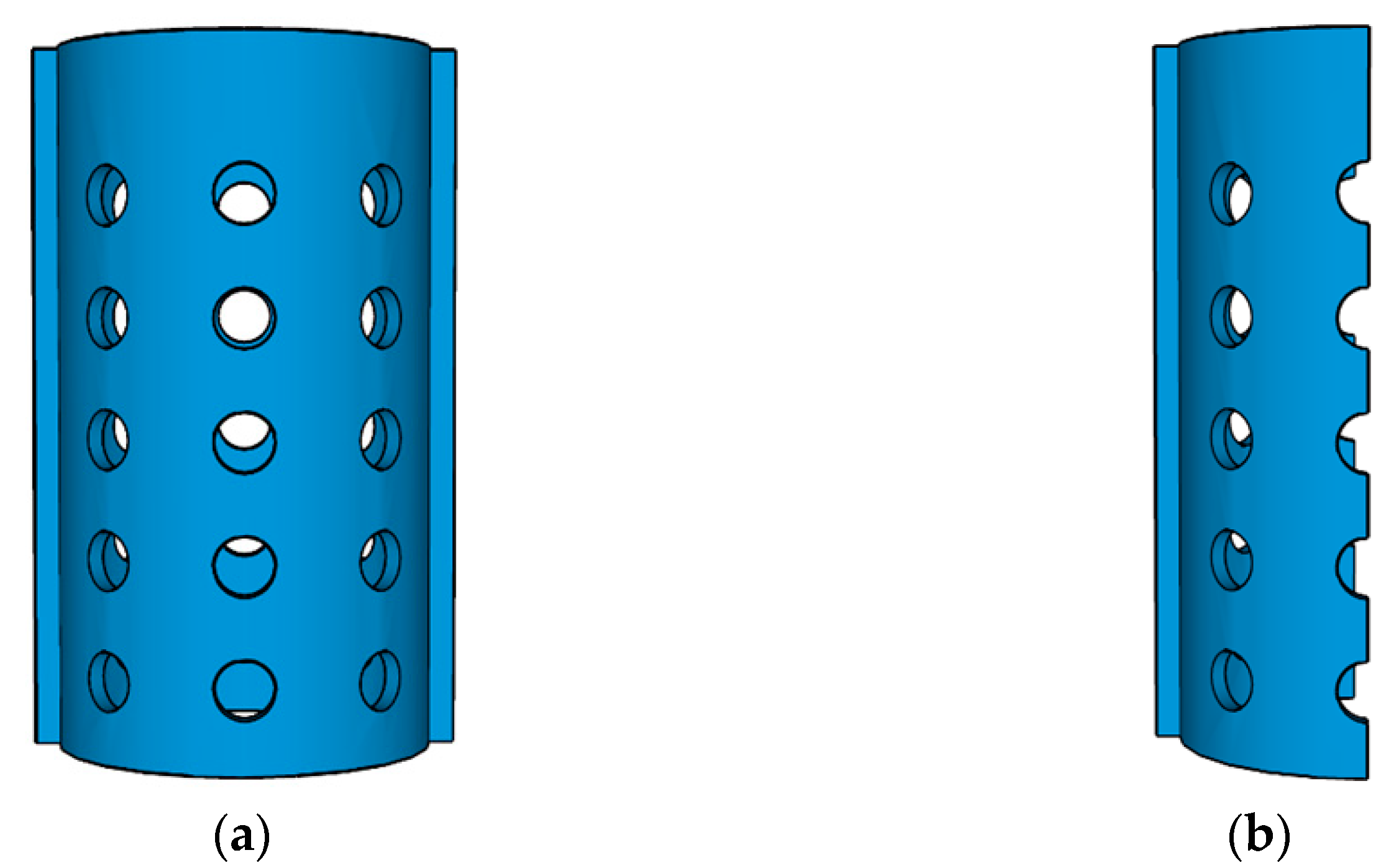
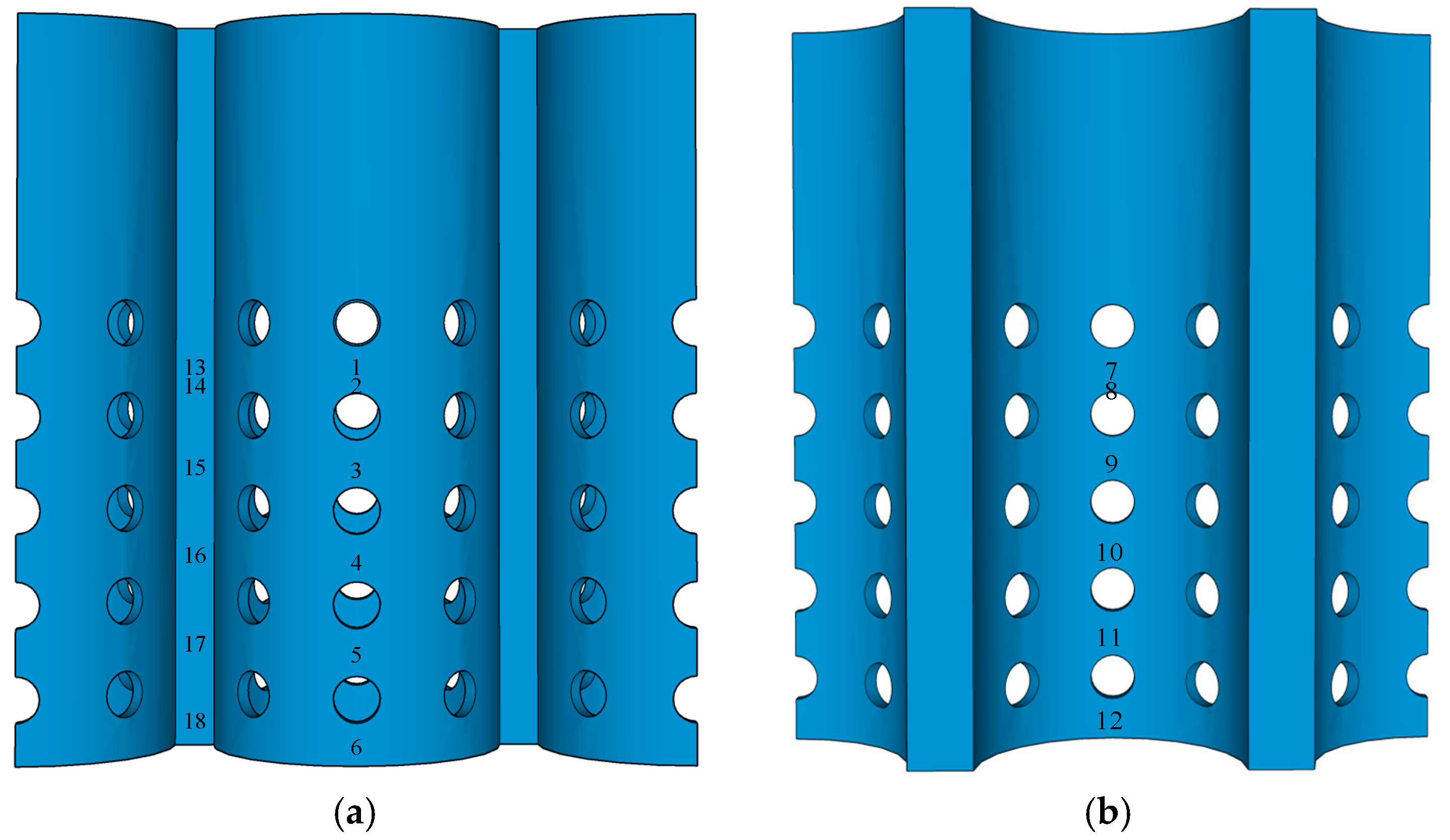
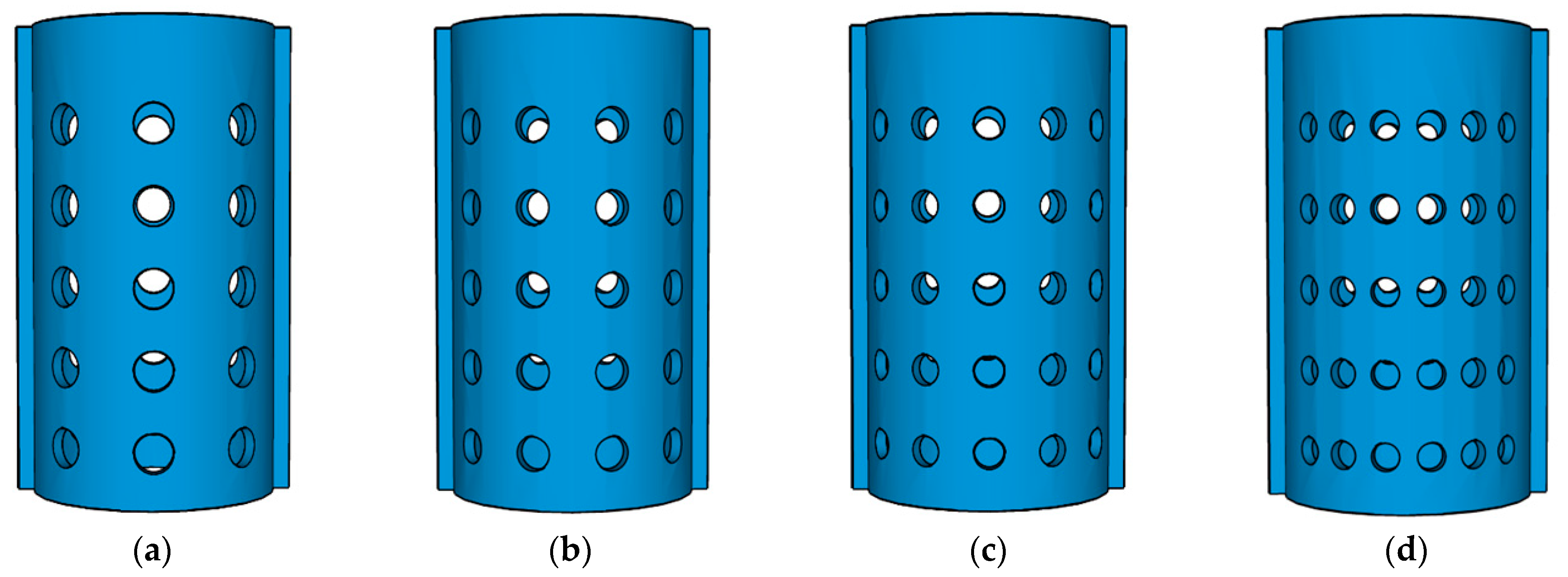
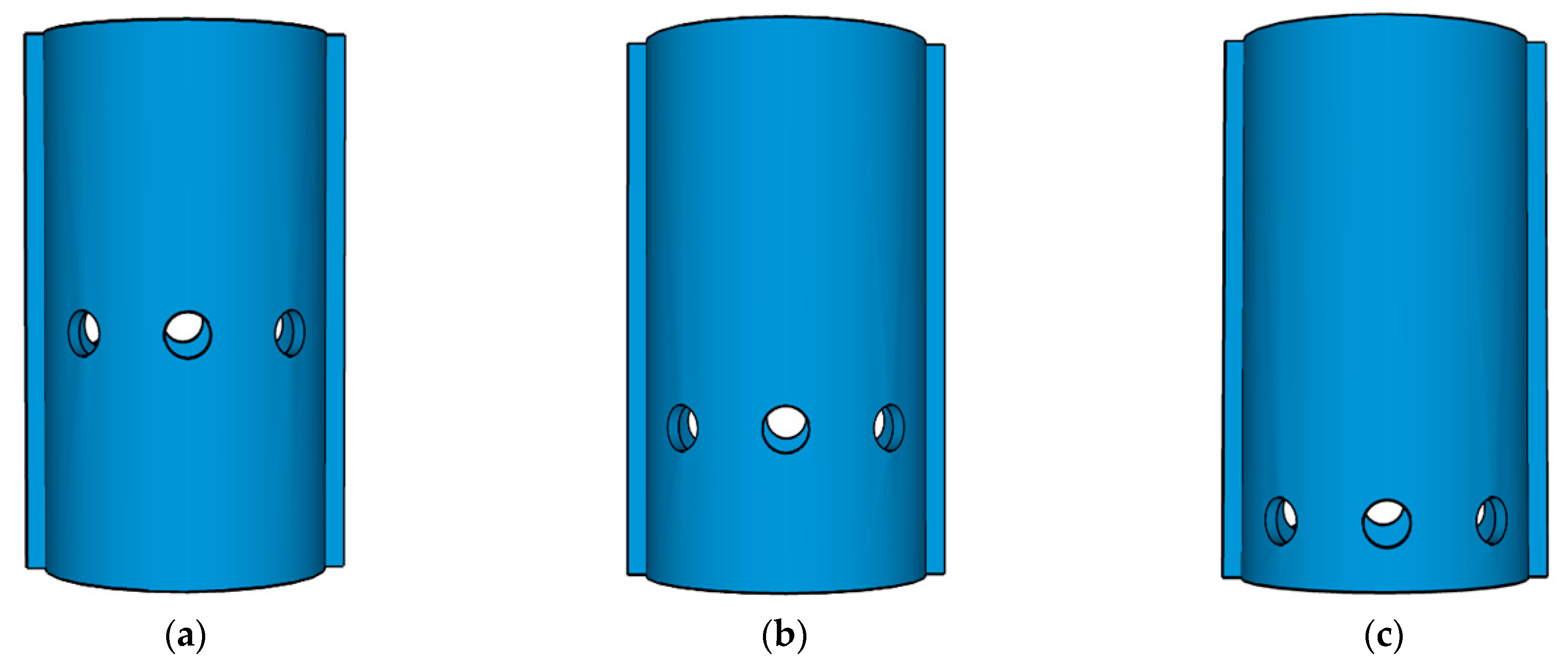
2.4. Structure Model

The structure model in this paper is based on the upper bucket part of the bucket-based structure in the Xuwei Port area of Lianyungang, Jiangsu Province, China. We scaled it down proportionally and perforated. Considering the structural dimensions of the model test flume, the parameters of the test equipment, and other performance factors, we determined the model scale of the bucket-shaped permeable breakwater was 1:28 according to the gravity similarity criterion. The model’s dimensions are as follows: outer diameter 0.32 m, inner diameter 0.29 m, height 0.6 m, connecting wall length 0.04 m, width 0.02 m. The center distance between any two openings in the depth direction is 0.1 m. Figure 3a shows the schematic diagram of the structure model. Given the structure model’s three-dimensional symmetry, the numerical flume’s front wall was specified as a symmetric boundary condition. We can fully represent the interaction between the waves and the structure model by calculating only half. Therefore, we correspondingly simplified the structure model in this study. Figure 3b shows the simplified model. The number of mesh elements was reduced from 2.58 million to 0.98 million through numerical model verification, and the calculation results were accurate, effectively improving computational efficiency. The simplification is reasonable.

3. Numerical Model Validation

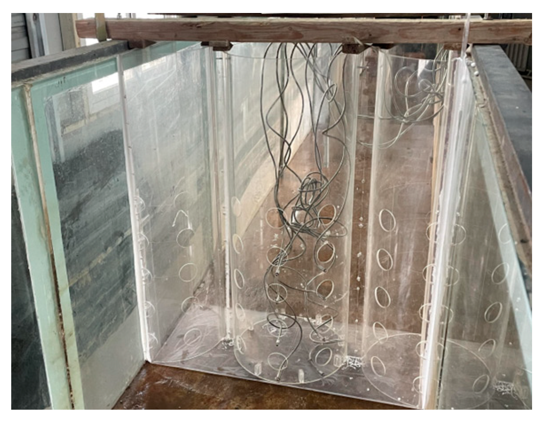
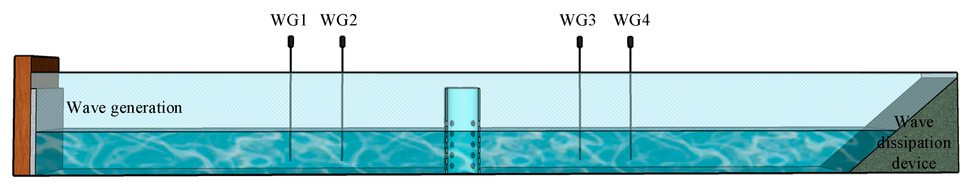
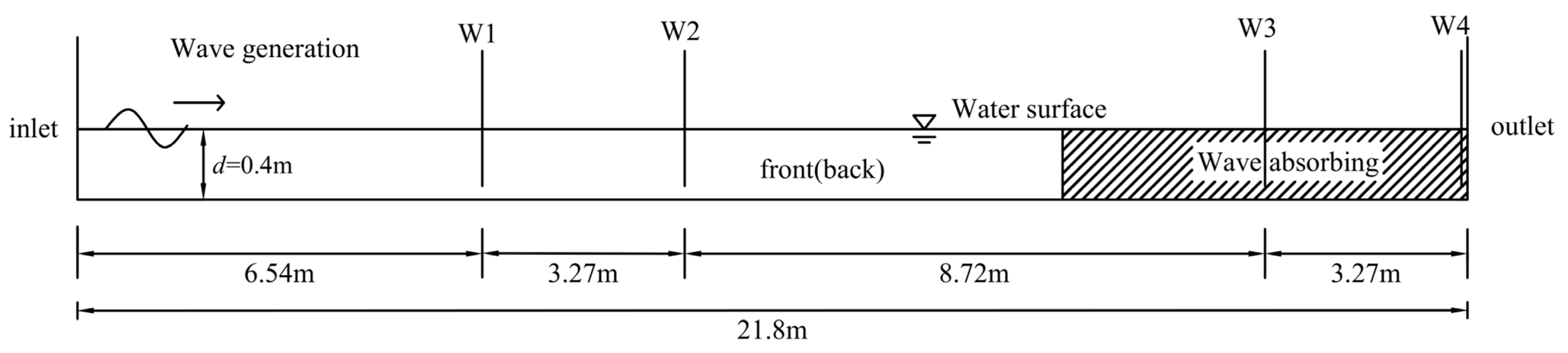
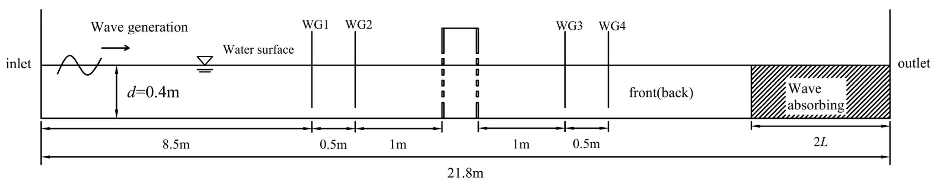
3.1. Physical Model Test Settings

The physical model test was carried out at the Coastal Engineering Laboratory of Dalian Ocean University. The dimensions of the flume are as follows: length 40 m, width 0.7 m, height 1 m. A servo-driven paddle wave generator is installed at the left end of the flume, with a width of 0.7 m, capable of generating regular waves with periods ranging from 0.5 s to 5 s. The end of the flume is equipped with energy dissipation devices such as a vertical dissipation frame and an overhead dissipative slope, which serve as the wave absorption zone for the model test.

Figure 4 shows the test model, which is identical in dimensions and structure to the structure model shown in Figure 3b. The specific dimensions are as follows: outer diameter 0.32 m, inner diameter 0.29 m, height 0.6 m, connecting wall length 0.04 m, width 0.02 m. The porosity of the test model is defined based on the “Code of Design for Breakwaters and Revetments JTS 154-2018” [36] for open caisson vertical breakwaters, which is the ratio of the open area to the total area between the upper and lower edges of the open part, and it is 12%. The center distance between any two openings in the depth direction is 0.1 m.

The arrangement of the pressure sensors on the model is designed based on the requirements of the “Technical Code of Modelling Test for Port and Waterway Engineering JTS/T 231-2021” [37] for wave model test point pressure sensor placement. Six measurement points are arranged from top to bottom at the most protruding part of the bucket wall on the wave-facing side and the centerline of the connecting wall, numbered sequentially from #1 to #6 and #13 to #18. Six measurement points are also arranged inside the bucket at the most concave part, numbered sequentially from #7 to #12. The distances of each measurement point from the bottom surface, from top to bottom, are 0.42 m, 0.4 m, 0.32 m, 0.22 m, 0.12 m, and 0.015 m. Figure 5 shows the specific arrangement. The model’s center is located at 10.16 m along the x-axis of the flume. Two wave height gauges are placed 1 m and 1.5 m in front of the model, and two wave height gauges are placed 1 m and 1.5 m behind the model to monitor the changes in the free surface of the water before and after the model. The water depth d is constantly maintained at 0.4 m. Figure 6 shows the specific layout of the model test flume.

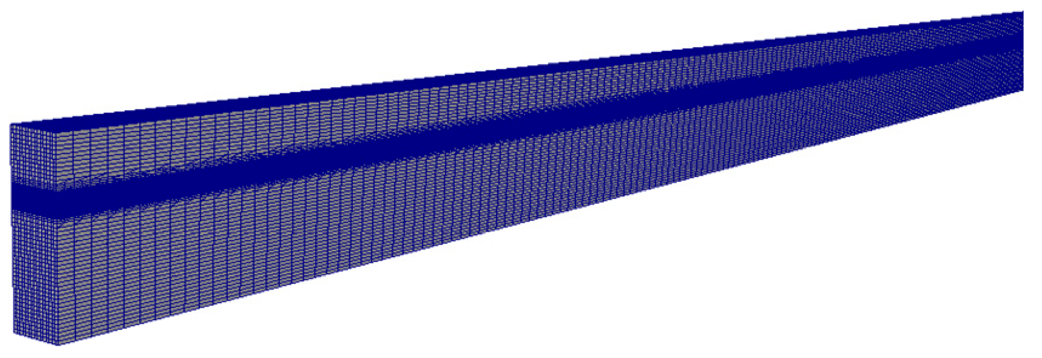
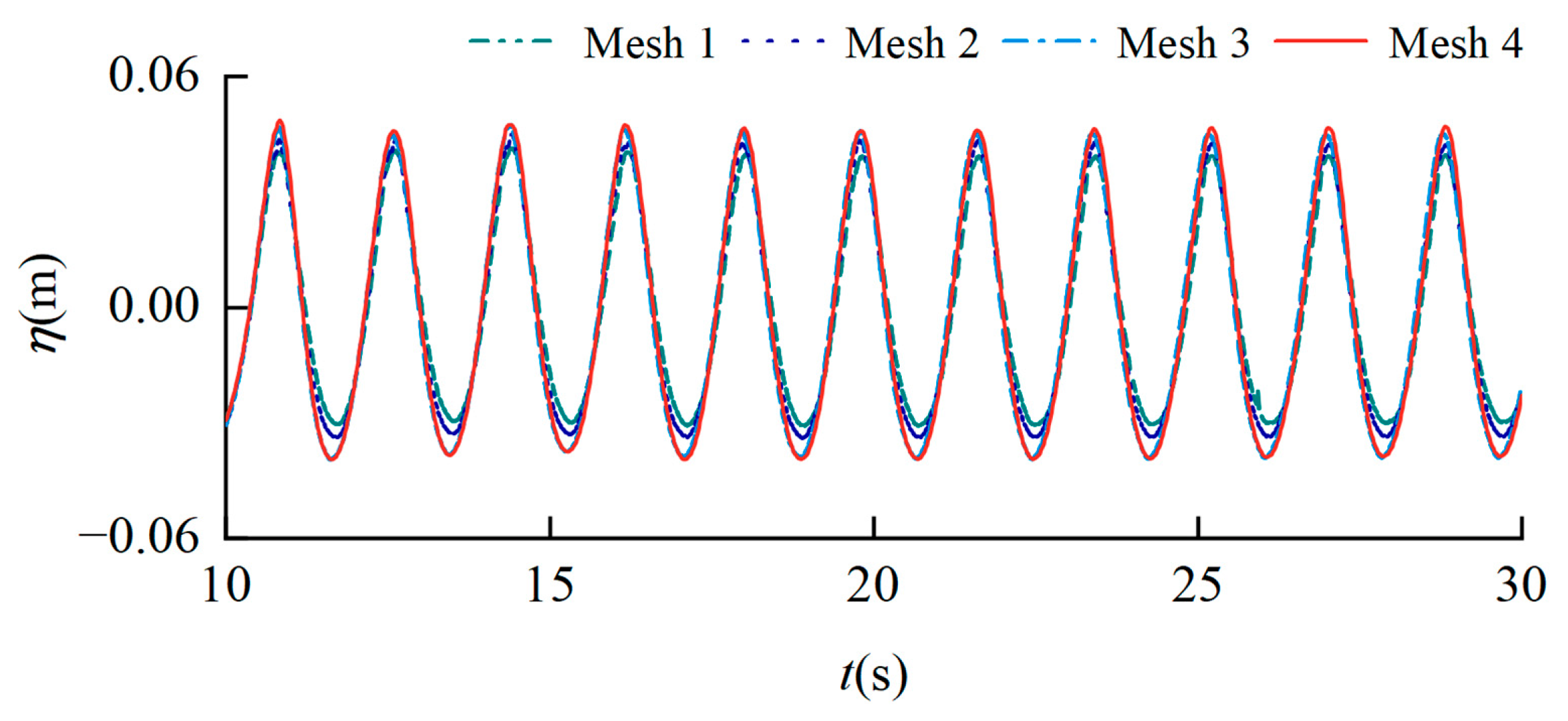
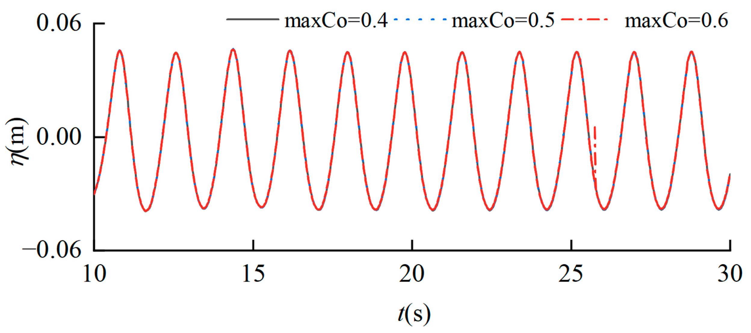
3.2. Spatiotemporal Verification

The dimensions of the three-dimensional numerical wave flume are as follows: length 21.8 m, width 0.18 m, and height 0.6 m, with a constant water depth d of 0.4 m. The wave parameters are set as follows: wave height H = 0.09 m and period T = 1.8 s. Symmetric boundary conditions are employed in this study to ensure that the numerical simulation accurately corresponds to the dimensions of the water flume after the structure is placed. The length of the damping wave dissipation zone is set to twice the wavelength. Two wave height gauges are positioned within the fluid domain of the flume at distances of two and three times the wavelength from the inlet boundary, with one at the middle and the other at the end of the damping wave dissipation zone. These gauges are used to verify the accuracy of the moving boundary wave generation and the effectiveness of the damping wave dissipation zone in attenuating waves. The wave height gauges are numbered sequentially from left to right as W1, W2, W3, and W4. Figure 7 illustrates the specific layout of the numerical empty wave flume.

This paper sets up four different grid scales to calculate the variation of wave elevation over time and examine the impact of grid density on numerical calculation results. Initially, the entire numerical flume with dimensions length × width × height is divided into background grids with scales of 0.12 m × 0.024 m × 0.024 m, 0.1 m × 0.02 m × 0.02 m, 0.06 m × 0.012 m × 0.012 m, and 0.045 m × 0.009 m × 0.009 m, respectively. Then, refinement is applied once in the height ranges of 0.3–0.5 m and 0.35–0.45 m. The incoming wave direction is defined as the x-direction, with Δx as the horizontal grid scale and N_x as the number of horizontal grids; the width direction of the flume is defined as the y-direction, with Δy as the width grid scale and N_y as the number of grids in the width direction; the vertical direction of the flume is defined as the z-direction, with Δz as the vertical grid scale and N_z as the number of grids in the vertical direction. Figure 8 shows the grid division of the numerical wave flume without structures.

Table 1. Grid parameters of different densities.

Case Number	$∆\mathit{x}\left(\mathbf{m}\right)$	${\mathit{N}}_{\mathit{x}}$	$∆\mathit{y}\left(\mathbf{m}\right)$	${\mathit{N}}_{\mathit{y}}$	$∆\mathit{z}\left(\mathbf{m}\right)$	${\mathit{N}}_{\mathit{z}}$	Cell Number
1	0.12	182	0.024	8	0.024	25	106,288
2	0.1	218	0.02	9	0.02	30	184,431
3	0.06	363	0.012	15	0.012	50	871,842
4	0.045	484	0.009	20	0.009	67	2,013,440

shows the grid parameters. Figure 9 shows the comparison results of wave elevation time history curves for different grid densities.

Table 2. Comparison of metrics related to grid errors.

Mesh	$\mathbf{Wave} \mathbf{Height} \mathbf{Error} {\mathit{\varphi }}_{\mathit{H}}$ (%)	$\mathbf{Wave} \mathbf{Period} \mathbf{Error} {\mathit{\varphi }}_{\mathit{T}}$ (%)
1	24.2	0.25
2	15.8	0.12
3	7.5	0
4	6.3	0

presents the comparison data for grid error metrics [38].

As shown in Figure 9 and Table 2, the calculation results of Grid 3 and Grid 4 are not significantly different. This indicates that when the flume’s base grid size is 0.06 m × 0.012 m × 0.012 m, the generated regular wave surface has already converged and meets the calculation accuracy requirements. Further grid refinement does not lead to significant changes in the calculation results. Therefore, to improve computational efficiency, this paper selects Grid 3 as the base grid for the numerical simulation of the flume.

Three different time steps were set up based on Grid 3 for verification, with the same conditions as before, to further verify the impact of the time step on calculation accuracy. Since this paper adopts a dynamic time step, the maximum Courant number was adjusted to vary the time step. The time step independence was verified for maximum Courant numbers of 0.4, 0.5, and 0.6. Figure 10 shows the comparison results of wave surface time history curves for different time steps.

As can be seen from the figure, when the maximum Courant number is set to 0.4 and 0.5, the wave surface is in a convergent state. When the maximum Courant number is set to 0.6, the wave surface becomes unstable around 26 s. Considering that a smaller time step may lead to an increase in the computation period and cost, while a larger time step may reduce the accuracy of numerical calculations, this paper selects a maximum Courant number of 0.5 for subsequent numerical calculations after comprehensive consideration.

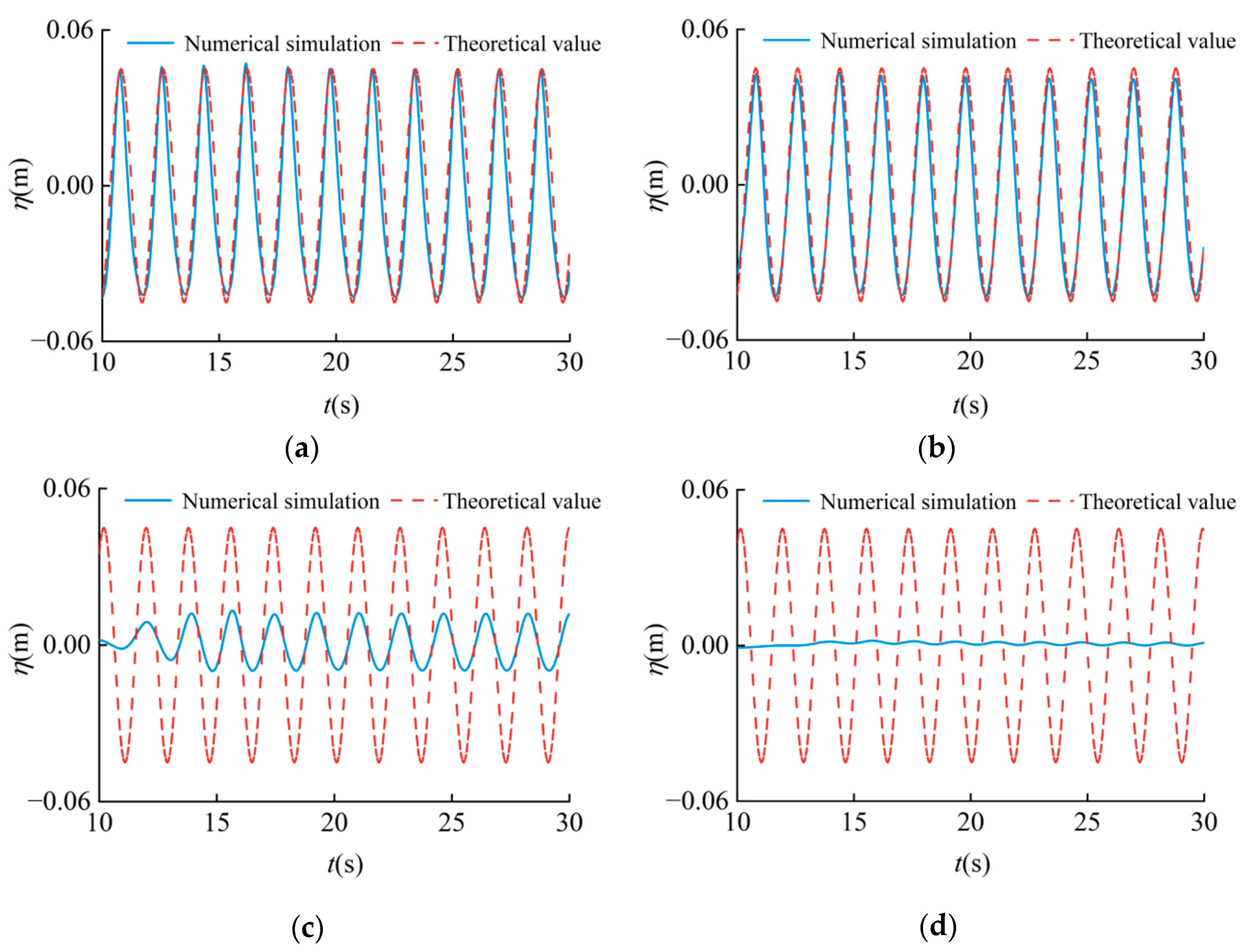
3.3. Wave Generation Validation

Figure 11 presents a comparison between the numerical calculation results of this paper and the analytical results of the linear wave theory. As can be seen from the figure, at positions two wavelengths (x = 6.54 m) and three wavelengths (x = 9.81 m) away from the inlet boundary, the numerically calculated wave surface shows good consistency with the theoretical wave surface. In the middle of the damping wave absorption zone (x = 18.53 m) and at the end of the flume (x = 21.7 m), the comparison between the numerically calculated wave surface and the theoretical wave surface demonstrates the effectiveness of the damping wave absorption zone in wave attenuation. In summary, the effectiveness of the numerical flume has been verified from a theoretical perspective.

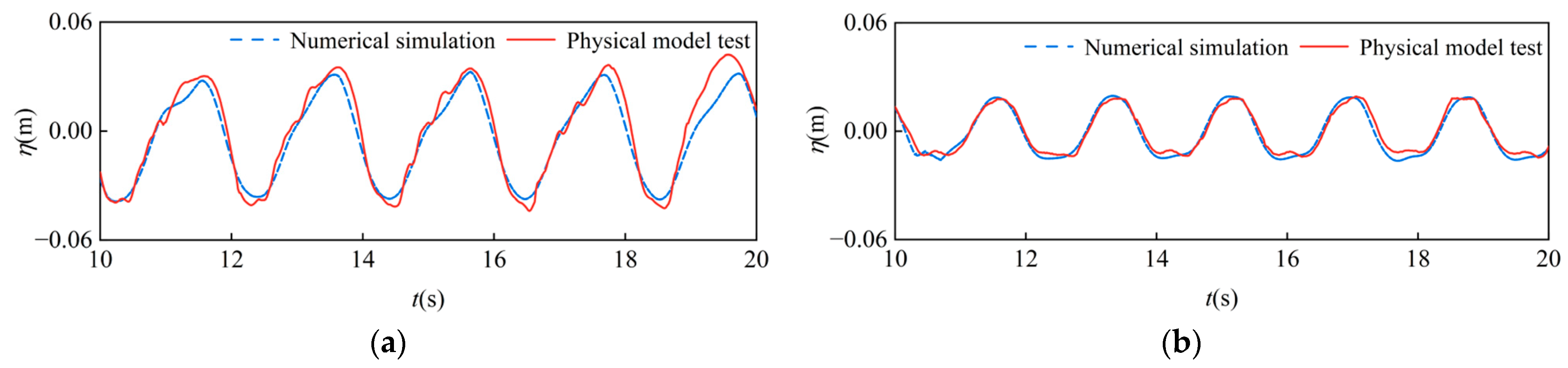
3.4. Model Test Verification

Figure 12 illustrates the detailed layout of the numerical simulation flume. After the model was incorporated, a comparative analysis was performed between the numerical calculation results and the physical model test results to further validate the numerical flume’s reliability.

Figure 13 compares the numerically calculated wave surface with the model experiment wave surface under the condition of H = 0.09 m and T = 1.8 s. In Figure 13a, the reflected wave surface is obtained by separating the data monitored by WG1 and WG2 using the Goda two-point method [39], and in Figure 13b, the transmitted wave surface is measured by WG3. By comparing the two wave surfaces, it can be seen that during the interaction between the waves and the experimental model, the numerically calculated reflected and transmitted wave surfaces both match well with the model experiment wave surfaces.

Table 3. Comparison of transmission coefficients results.

T/s	H = 0.11 m		H = 0.09 m		H = 0.07 m
	Numerical Simulation	Physical Model Test	Numerical Simulation	Physical Model Test	Numerical Simulation	Physical Model Test
1.2	0.32	0.30	0.34	0.32	0.39	0.36
1.4	0.34	0.32	0.39	0.35	0.42	0.38
1.6	0.35	0.34	0.39	0.37	0.40	0.40
1.8	0.37	0.36	0.40	0.40	0.45	0.44
2.0	0.39	0.37	0.42	0.39	0.46	0.44

and

Table 4. Comparison of reflection coefficients results.

T/s	H = 0.11 m		H = 0.09 m		H = 0.07 m
	Numerical Simulation	Physical Model Test	Numerical Simulation	Physical Model Test	Numerical Simulation	Physical Model Test
1.2	0.49	0.50	0.46	0.47	0.42	0.45
1.4	0.54	0.56	0.51	0.51	0.46	0.48
1.6	0.54	0.55	0.5	0.5	0.48	0.48
1.8	0.59	0.61	0.54	0.56	0.50	0.53
2.0	0.58	0.60	0.54	0.58	0.51	0.55

present the transmission and reflection coefficients obtained from numerical simulations and physical model tests. Figure 14 compares the reflection, transmission, and dissipation coefficients obtained from numerical calculations and model tests for the bucket-shaped permeable breakwater with a porosity of 12% at relative wave heights H/d of 0.275, 0.225, and 0.175. The horizontal axis represents the relative wavelength L/D (where L is the wavelength and D is the inner diameter). The numerical calculation results match well with the model test results, with errors within a reasonable range of 10%. The analyzed error between the two is mainly due to the placement of the pressure sensor connection lines inside the bucket during the model test, which increased wave reflection and decreased wave transmission. Therefore, it is easy to explain why the reflection coefficients measured in the model test are generally higher while the transmission coefficients are usually lower.

Figure 15 shows the comparison of wave pressure time histories at the locations of pressure measurement points 1 to 18 for a bucket-shaped permeable structure with H = 0.09 m and period T = 1.8 s between numerical simulation results and physical model test results. The data results indicate that the numerical calculation results at each measurement point match well with the physical model test results.

Through the above spatial and temporal verification, wave generation validation, and model test verification, we can see the three-dimensional numerical wave flume constructed in this paper can effectively simulate the interaction between waves and the bucket-shaped permeable structure. The obtained calculation results are accurate and reliable.

4. Hydrodynamic Characteristics of Bucket-Shaped Permeable Breakwater

4.1. Numerical Simulation Parameter Settings

From the model test and numerical simulation results (Figure 14), we can see that within the scope of this study, with a fixed relative wave height, changes in wavelength have a limited impact on the reflection and transmission coefficients of the bucket-shaped permeable structure. Due to space limitations, the subsequent research in this paper is conducted using L = 3.27 as a representative case, and

Table 5. Operational parameter settings.

Parameters	Specific Values
Water depth d/m	0.4
Period T/s	1.8
Wavelength L/m	3.27
Wave height H/m	0.07/0.09/0.11
Opening ratio e/%	4.6/8/12/17/23
Number of openings/unit	3/4/5/6
Opening center position/m	0.27/0.17/0.07

presents the relevant working condition parameters.

4.2. The Effect of Porosity on Wave Dissipation Performance

Figure 16a–c compare the bucket-shaped permeable breakwater’s reflection, transmission, and dissipation coefficients with different porosities at relative wave heights H/d of 0.275, 0.225, and 0.175, respectively. As can be seen from the figures, the reflection coefficient of the bucket-shaped permeable breakwater shows a negative correlation with the porosity e, the transmission coefficient shows a positive correlation with the porosity, and the relationship between the dissipation coefficient and the porosity shows a trend of first positive correlation and then negative correlation, reaching a maximum value at a porosity of 12%. This suggests that the bucket-shaped permeable breakwater achieves its most robust energy dissipation performance at a porosity of 12%. At this porosity level, the interaction between the waves and the openings and the breakwater’s interference with the waves reaches an optimal balance. However, when the porosity exceeds a specific critical value (12% in this study), the increased openings significantly enhance the structure’s permeability, allowing more wave energy to pass directly through the breakwater without effective dissipation. As a result, wave energy is transmitted directly rather than reduced through structural dissipation. Consequently, although the transmission coefficient increases, the actual energy dissipated within the structure decreases, reducing the overall dissipation coefficient. Furthermore, when the porosity is too high, the breakwater’s ability to interfere with the waves diminishes, reducing the interaction between the waves and the structure. This reduction in wave reflection and refraction within the structure further decreases the energy dissipation efficiency of the breakwater.

In summary, after evaluating the overall performance of the bucket-shaped permeable structure in terms of wave reflection, transmission, and dissipation, we conclude that the bucket-shaped permeable breakwater with a 12% porosity demonstrates the optimal wave dissipation performance. The optimal wave dissipation performance here refers to comprehensive dissipation performance. We should determine the appropriate porosity in practical applications based on specific usage requirements. We should select a higher porosity value if we focus on reducing wave pressure, wave reflection, and water exchange inside and outside the harbor. If the focus is on maintaining calm waters inside the harbor, we should select a lower porosity value.

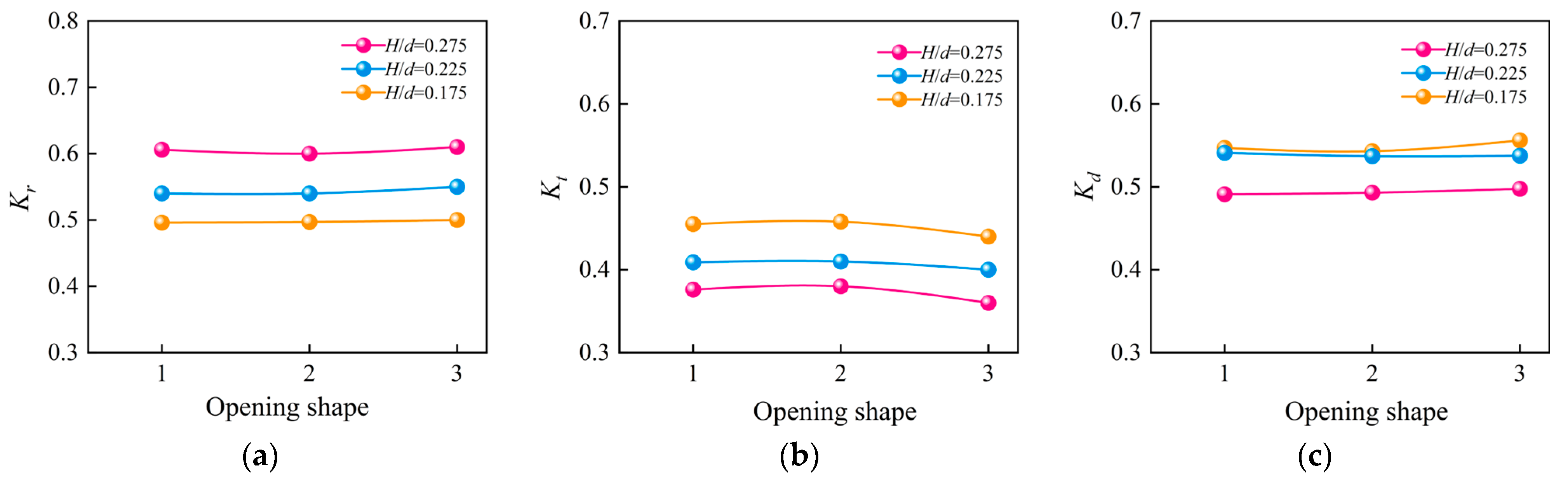
4.3. The Effect of Opening Shape on Wave Dissipation Performance

The design of the opening shapes is based on a bucket-shaped permeable breakwater with a porosity of 12%. The schematic diagrams of the buckets with different opening shapes are shown in Figure 17. For convenience, this paper assigns the circular, square, and rectangular openings as No. 1, No. 2, and No. 3, respectively, corresponding to the schematic diagrams Figure 17a–c. Figure 18 sequentially presents the impact of different opening shapes on the bucket-shaped permeable breakwater’s reflection, transmission, and dissipation coefficients. As shown in the figure, at a porosity of 12%, altering the shape of the openings has minimal impact on the reflection, transmission, and dissipation coefficients during the interaction between the bucket-shaped permeable breakwater and waves. This result suggests that, at a specific porosity, the geometric shape of the openings does not significantly influence the reflection, transmission, or dissipation of wave energy. Further analysis indicates that the reflection coefficient rises for the exact opening shape as the relative wave height increases while the transmission and dissipation coefficients decrease. This implies that more wave energy is reflected back at higher wave heights, with less energy being transmitted or dissipated. These findings highlight that wave height is critical in the interaction between waves and the bucket-shaped permeable breakwater. In contrast, the shape of the openings plays a relatively minor role.

Given the minimal differences in wave dissipation effectiveness among various opening shapes, designers can select the most appropriate opening shape for the bucket-shaped permeable breakwater based on specific engineering requirements and constraints without significant concern for its impact on dissipation performance. This flexibility not only facilitates the optimization of structural design but also helps reduce construction costs, thereby enhancing the overall economic efficiency and feasibility of the project.

4.4. The Effect of the Number of Openings on Wave Dissipation Performance

Under a 12% porosity of the bucket, the total open area remains unchanged by varying the area of individual openings to achieve a change in the number of openings. Figure 19a–d illustrate the bucket-shaped structures with different numbers of openings.

Table 6. Mesh resolution values.

Structural Configuration	$\mathbf{Opening} \mathbf{Diameter} \mathit{\phi }$ (m)	z$-\mathbf{Direction} \mathit{\phi }/{\mathit{h}}_{\mathit{z}}$	y$-\mathbf{Direction} \mathit{\phi }/{\mathit{h}}_{\mathit{y}}$
Figure 19a	0.05	16.7	16.7
Figure 19b	0.0433	14.4	14.4
Figure 19c	0.0387	12.9	12.9
Figure 19d	0.0354	11.8	11.8

presents detailed data for the opening diameter $\phi$ and the mesh resolution in different directions (the ratio of the opening diameter to the unit mesh size, with the mesh size represented by ‘h’ in this paper). Figure 20a–c, respectively, compare the reflection coefficient, transmission coefficient, and dissipation coefficient of waves on the bucket-shaped permeable breakwater with different numbers of openings at relative wave heights H/d of 0.275, 0.225, and 0.175. We can see from the figures that changing the number of openings under 12% porosity has almost no effect on the reflection, transmission, and dissipation coefficients of wave action on the bucket-shaped permeable breakwater. This result indicates that increasing the number of openings does not necessarily lead to greater fluid flow through the bucket-shaped permeable breakwater. In other words, even with a higher number of openings, the structure’s fluid transmission characteristics remain unchanged due to the constant total opening area. From a scale effect perspective, the size of each opening is relatively small compared to the wave scale, which limits its impact on wave transmission and dissipation. Whether the number of openings is increased or decreased, the overall wave dissipation performance remains largely unaffected. This is because the interaction between the waves and the openings is primarily governed by the total opening area rather than the number of openings.

In summary, under the condition of a constant porosity of the bucket, changes in the shape and number of openings have no significant effect on the waves’ reflection, transmission, and dissipation coefficients. In practical applications, we can flexibly determine the shape and number of openings based on the stress-strain conditions of the perforated bucket, the ease of construction, and the aesthetic requirements of the external appearance.

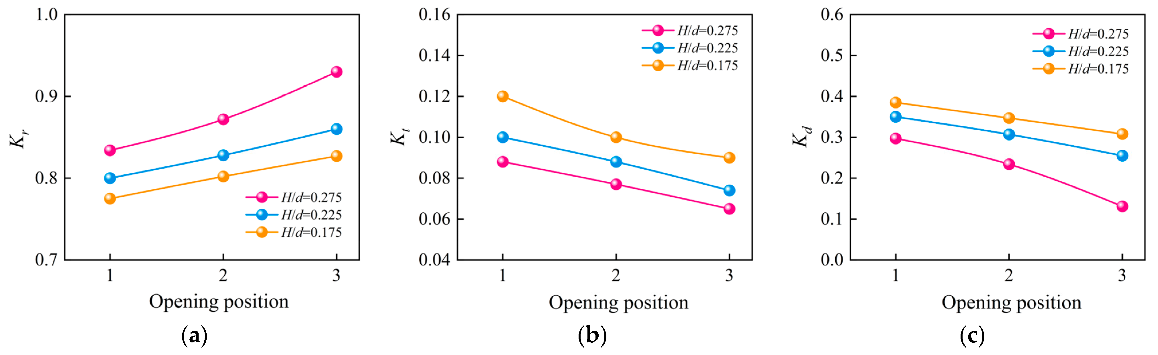
4.5. The Effect of Opening Position on Wave Dissipation Performance

We created three designs with different opening center heights under constant porosity to explore the impact of opening position on the wave dissipation performance of bucket-shaped permeable breakwaters. Each design has three openings on the bucket-shaped permeable breakwater’s front and back walls, with an opening diameter of 0.05 m. The opening center heights are 0.27 m, 0.17 m, and 0.07 m, respectively, and are sequentially numbered as No. 1, No. 2, and No. 3, corresponding to schematic Figure 21a–c. Figure 21 shows the buckets with different opening positions. The reflection, transmission, and dissipation coefficients of the bucket-shaped permeable breakwater under the conditions of T = 1.8 s, H/d = 0.275, H/d = 0.225, and H/d = 0.175 are shown in Figure 22. The figure demonstrates that as the height of the openings increases, the wave reflection coefficient of the bucket-shaped permeable breakwater decreases while the transmission and dissipation coefficients increase. This suggests that higher-positioned openings are more effective at reducing wave reflection and enhancing the transmission and dissipation of wave energy. The likely reason is that waves interacting with higher openings have more opportunities to transmit energy through the structure, thereby reducing reflection and enabling more efficient energy dissipation. Moreover, when fixing the opening position, changes in relative wave height significantly influence wave reflection, transmission, and dissipation. The reflection coefficient rises as the relative wave height increases, while the transmission and dissipation coefficients decrease. This may occur because, under higher wave conditions, wave energy is more prone to reflection rather than transmission or dissipation.

The study results suggest that in practical engineering, if the goal is to reduce wave reflection in front of the bucket-shaped structure to minimize the impact on the adjacent coastline, positioning the openings higher is an effective strategy. Higher openings can more effectively transmit wave energy, thereby reducing the formation of reflected waves. If the objective is to minimize wave penetration through the bucket-shaped structure, such as when protecting the interior of a harbor, the openings should be positioned lower. Lower openings help to confine wave energy in front of the structure, reducing transmission and enhancing protection. However, we recommend positioning the openings higher if the aim is to reduce reflection and increase energy dissipation. This approach maximizes wave energy dissipation and provides a more balanced wave management solution.

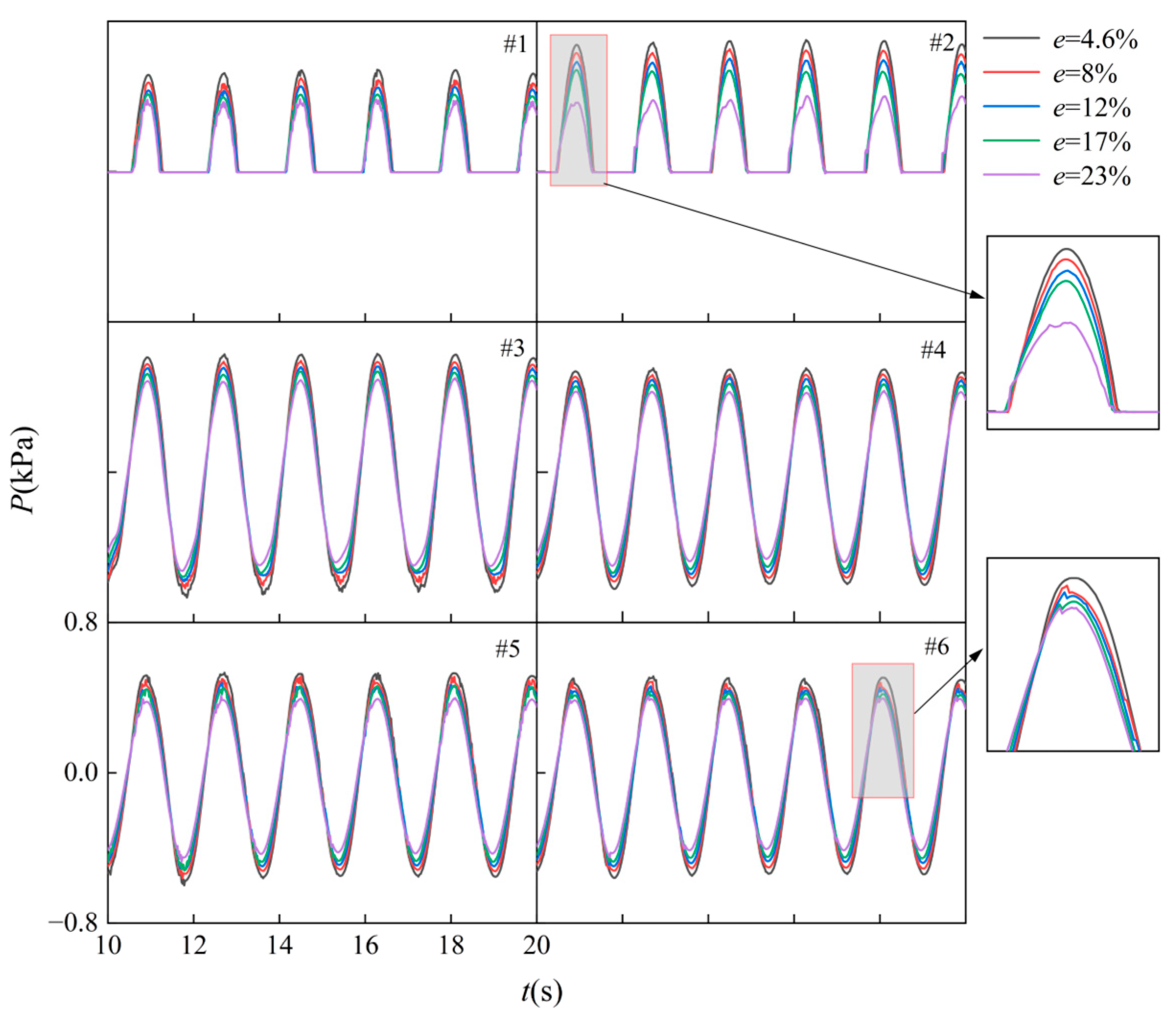
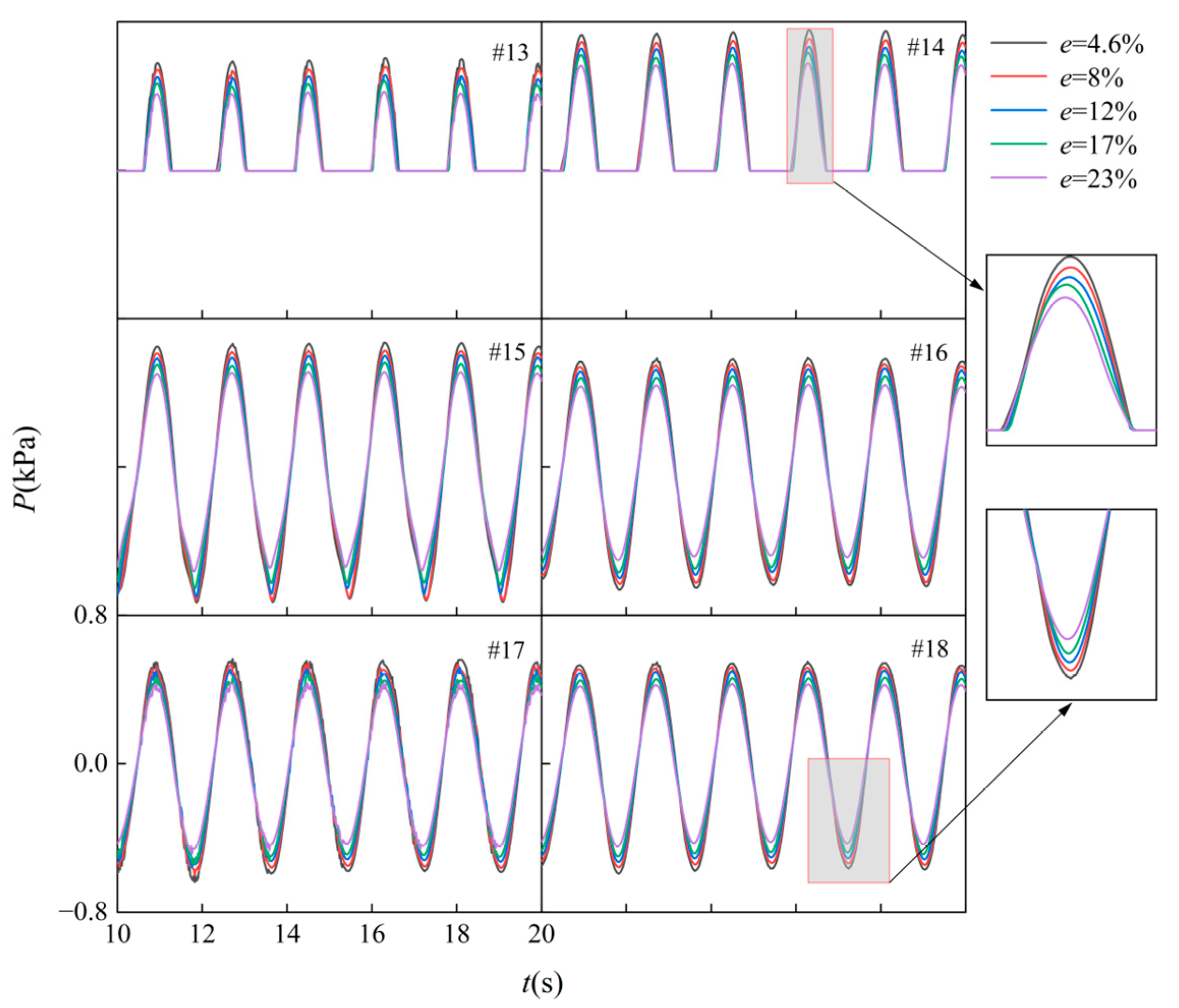
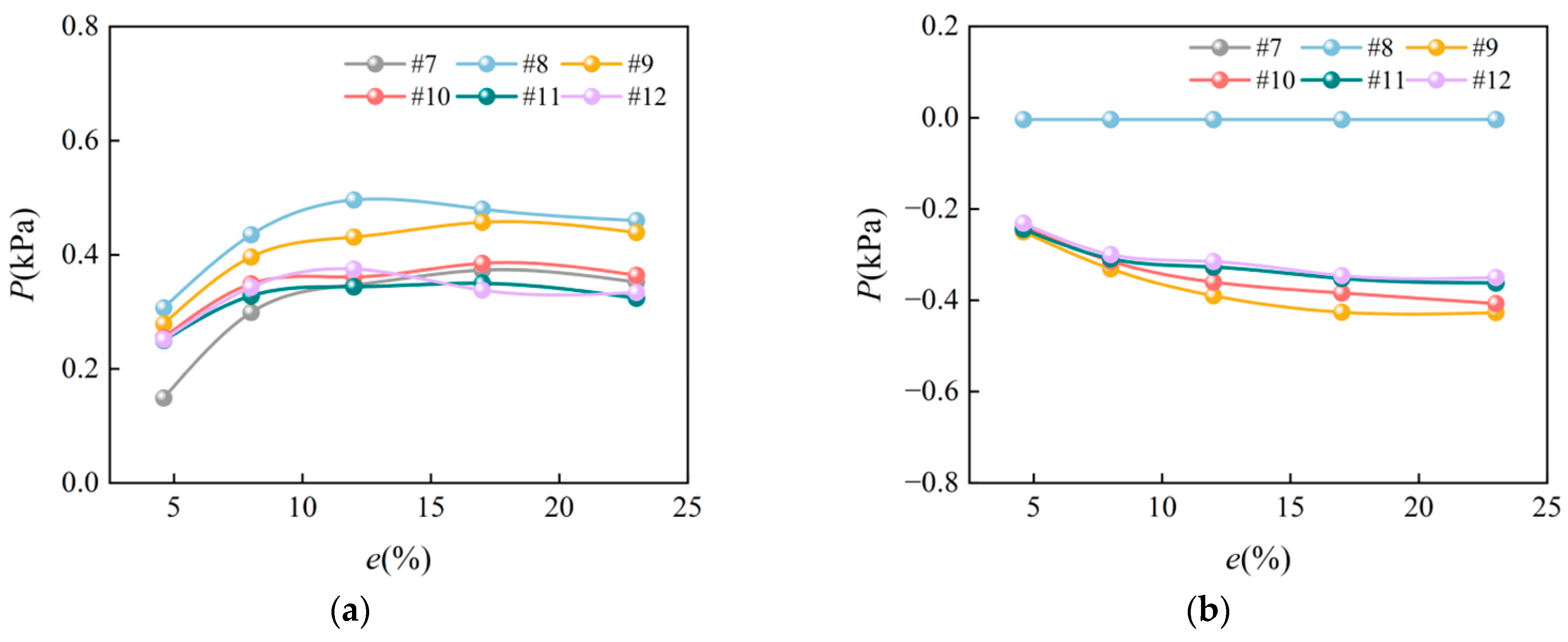
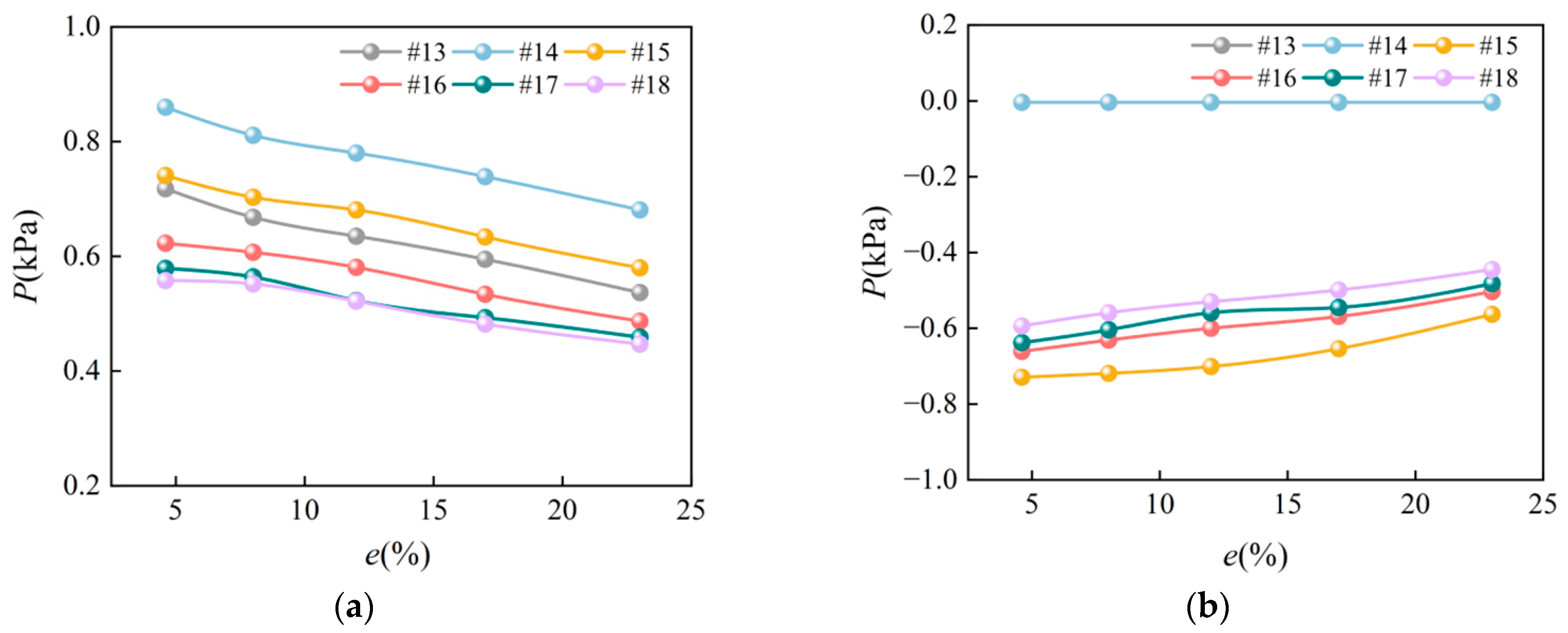
4.6. The Effect of Porosity on Wave Pressure

Under relative wave height H/d = 0.225 and T = 1.8 s conditions, Figure 23 compares pressure time-history curves at measurement points #1 to #6 on the bucket-shaped permeable breakwater with different porosities. Figure 24 presents the curves for measurement points #7 to #12, and Figure 25 provides the curves for measurement points #13 to #18. Measurement points #1 to #6 are located at the most convex part of the front wall on the wave-facing side, points #7 to #12 are at the most concave part of the inner wall, and points #13 to #18 are at the connecting wall (as shown in Figure 5).

The figures indicate that as the bucket’s porosity increases, the pressure curves’ peak values at measurement points #1 to #6 and #13 to #18 on the wave-facing side gradually decrease. This is because the increased porosity reduces the contact area between the bucket-shaped permeable breakwater and the incoming waves, weakening the reflected wave energy on the breakwater surface and reducing the pressure exerted by the reflected waves on the wave-facing side. Consequently, the pressure at the wave-facing measurement points decreases.

For measurement points #2 to #6, #8 to #12, and #14 to #18, the wave pressure on the bucket-shaped permeable breakwater decreases with increasing measurement point numbers. Measurement points #2, #8, and #14 are located at the still water level, where the interaction force between the waves and the breakwater is the greatest, resulting in the highest wave pressure. In contrast, measurement points #6, #12, and #18 are located at the bottom of the breakwater, where the impact of the waves is weaker, resulting in the lowest pressure.

To further analyze the variation patterns of the maximum positive and negative pressures at each measurement point, Figure 26. shows the comparison of the maximum positive and negative pressures at points #1 to #6 under different porosity conditions, with a relative wave height H/d = 0.225 and a wave period T = 1.8 s. From Figure 26a, we can see within the scope of this study that the maximum positive pressure at points #1 to #6 is negatively correlated with the porosity of the cylinder. The extreme value of the maximum positive pressure appears at point #2, with a value of 0.78 kPa. The reduction in maximum positive pressure for points #3 and #4 as the porosity increases is minimal, with both values decreasing by 16.8%. This indicates that the porosity affects the wave pressure at these two points less. Figure 26b. shows that the maximum negative pressure values at points #1 and #2 are zero. This is because point #1 is located just above the still water level and point #2 is at the still water level. When the wave trough reaches the structure’s wall, these points have no impact. The maximum negative pressure absolute values at points #3 to #6 are also negatively correlated with the porosity, with the extreme value appearing at point #3 at 0.67 kPa.

Figure 27 compares the maximum positive and negative pressures at measurement points #7 to #12 under different porosities. From Figure 27a, we can see within the scope of this study that the maximum positive pressure at points #7 to #12 inside the bucket-shaped permeable breakwater initially increases and then decreases as the porosity increases. The maximum positive pressures at points #8 and #12 reach their peak values at a porosity of 12%, with point #8 exhibiting an extreme value of 0.5 kPa. This indicates that at this porosity, waves may have experienced intense collisions at the still water level and the bottom of the inner wall on the rear side of the bucket. This finding further confirms, from a mechanical perspective, that the bucket-shaped permeable breakwater with a porosity of 12% has the most robust wave attenuation and dissipation performance. From Figure 27b, we can see a certain regularity between the maximum negative pressure absolute values and the porosity of the bucket. Specifically, as the porosity increases, the maximum negative pressure absolute values at points #9 to #12 inside the bucket also increase. This is because increased porosity reduces the energy of the reflected waves, resulting in less wave energy being reflected into the bucket-shaped permeable breakwater, thereby decreasing the positive pressure inside and increasing the negative pressure.

Figure 28 shows the maximum positive and negative pressures at measurement points #13 to #18 under different porosities. Figure 28a indicates that within the scope of this study, the maximum positive pressure at points #13 to #18 is negatively correlated with the perforation rate of the bucket. The maximum positive pressure appears at point #14, reaching 0.86 kPa, the highest among all pressure measurement points. Figure 28b shows that the maximum negative pressure absolute value at points #13 to #18 also negatively correlates with the porosities. The maximum negative pressure absolute value occurs at point #15, with a value of 0.73 kPa, which is also the highest among all pressure measurement points. Thus, we can see the maximum positive and negative pressures at the measurement points on the connecting wall of the bucket-shaped permeable breakwater and the most protruding part of the wave-facing side of the bucket show a consistent trend with the perforation rate of the bucket. Moreover, the connecting wall position experiences the highest wave pressure.

5. Conclusions

This paper takes the bucket-based breakwater in the Xuwei Port area of Lianyungang, Jiangsu Province, China, as a prototype and proposes a new type of bucket-shaped permeable breakwater. A three-dimensional numerical wave flume was established based on the OpenFOAM platform, and the open-source computational fluid dynamics toolbox DXFlow, previously developed by the project team, was utilized. After verifying the effectiveness of the numerical wave flume through spatiotemporal verification, wave generation validation, and model test verification, we studied the hydrodynamic characteristics of the bucket-shaped permeable breakwater under regular wave action. The research results indicate:

• The three-dimensional numerical wave flume based on OpenFOAM constructed in this paper can effectively simulate the interaction process between waves and the bucket-shaped permeable breakwater.
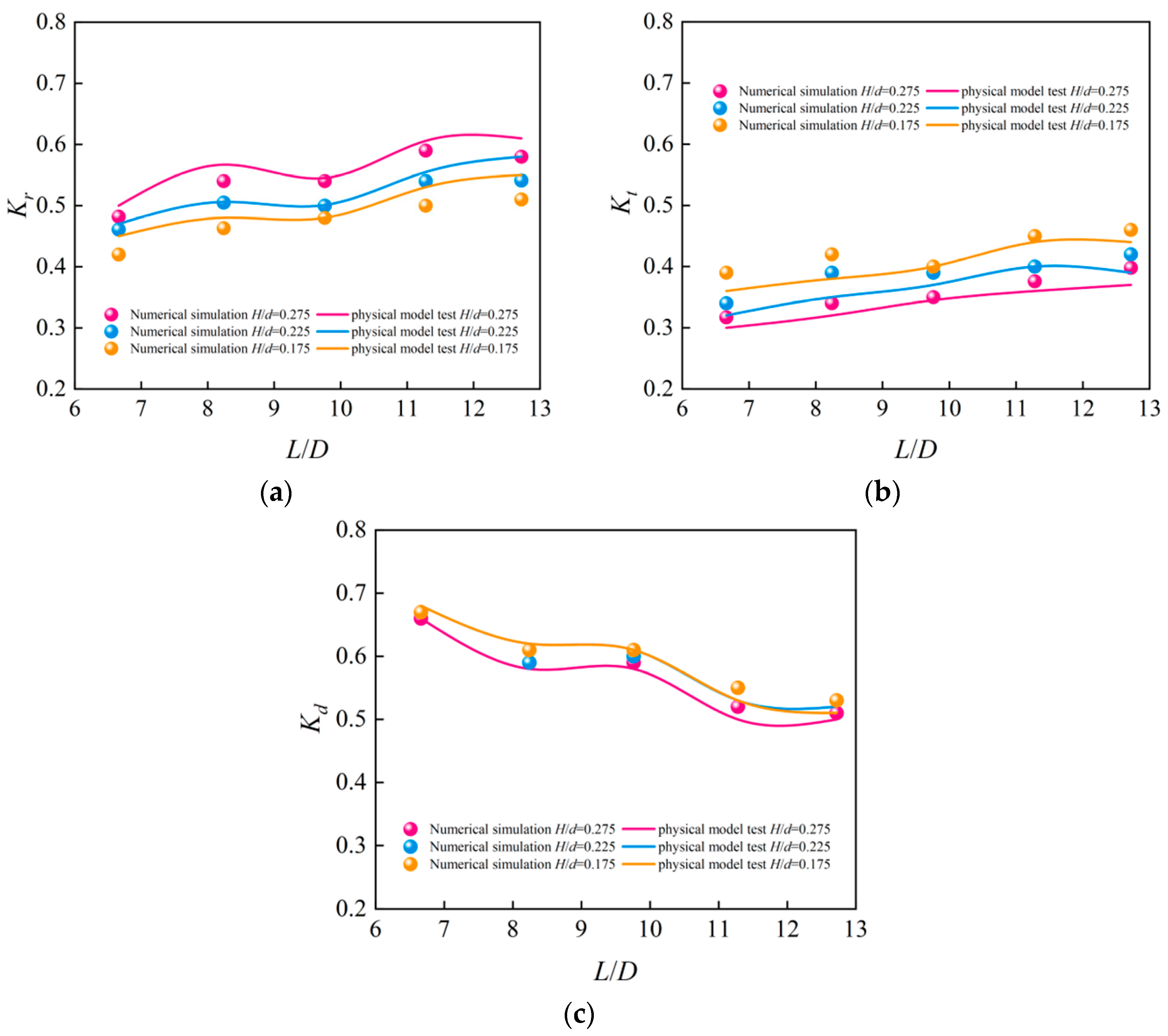
• Within the range of relative wavelength L/D between 6.7 and 12.7, relative wave height H/d between 0.175 and 0.275, changes in wavelength had a limited impact on the wave-dissipating performance of the bucket-shaped permeable breakwater. This indicates that the bucket-shaped permeable breakwater with this porosity has a stable wave dissipation effect within a specific wavelength range. When designing this type of breakwater, it is possible to consider a broader range of wave conditions, reducing the dependence on precise wave condition predictions, lowering design and maintenance costs, and enhancing the safety of coastal areas.
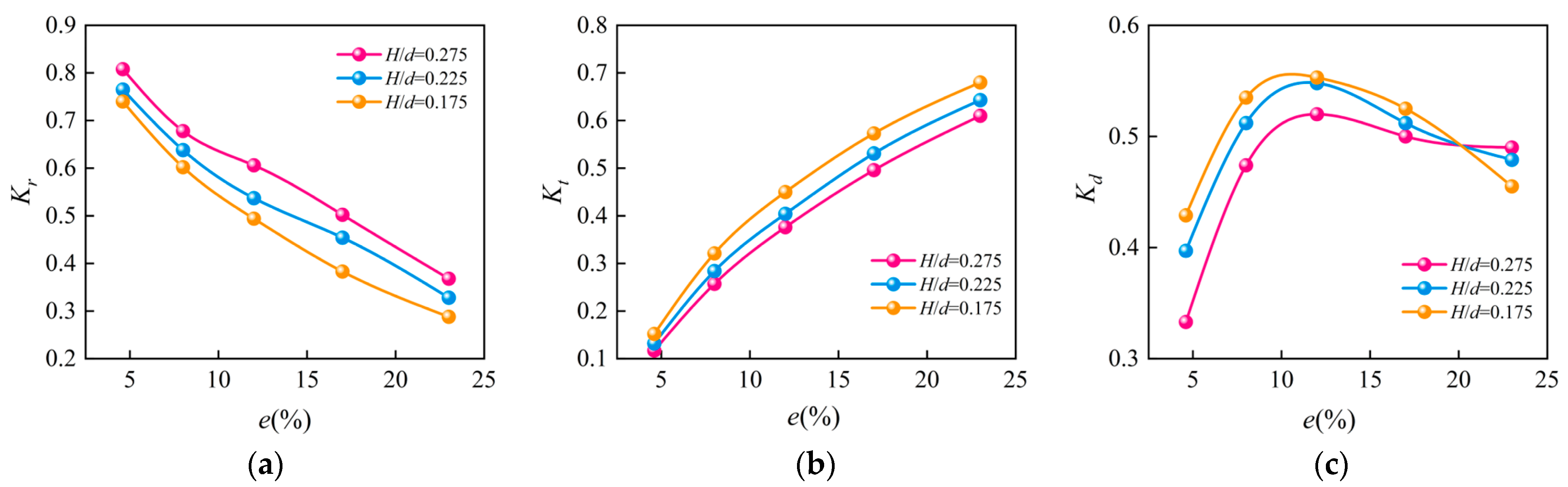
• When the bucket porosity is 12%, the dissipation coefficient reaches its maximum value, indicating that the bucket-shaped permeable breakwater has the best overall wave dissipation performance at this porosity. If the focus is on reducing wave pressure, wave reflection, and water exchange between the inside and outside of the port, a higher porosity is preferable. A lower porosity is advisable if the focus is on maintaining calm waters within the port.
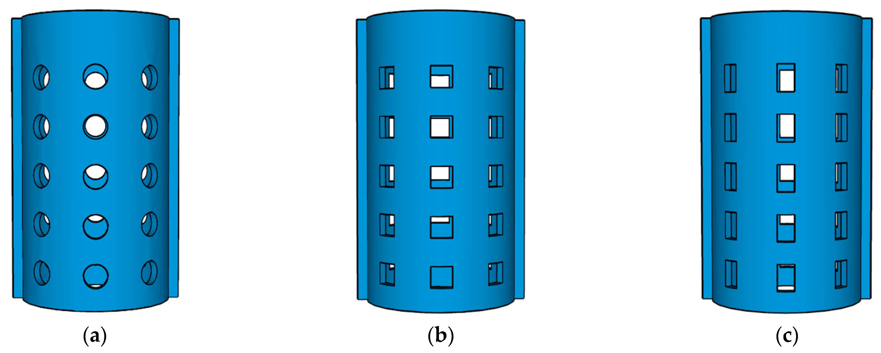
• The wave dissipation performance of the bucket-shaped permeable breakwater mainly depends on the porosity and is less related to the shape and number of openings. In practical applications, we can flexibly determine the shape and number of openings based on the stress-strain condition after perforation, construction difficulty, and aesthetic requirements.
• Higher opening positions help reduce wave reflection and increase wave energy transmission and dissipation within the structure, thereby reducing the impact of waves on the surrounding coastline. In practical engineering, we can adjust the wave dissipation effect of the structure by changing the opening positions to meet specific project requirements. For example, higher opening positions are preferable to reduce wave reflection in front of the bucket, and lower opening positions are preferable to minimize wave transmission through the bucket. For overall wave dissipation performance, higher opening positions are advisable.
• The connecting wall of the bucket-shaped permeable breakwater experiences the most significant wave impact. In practical engineering applications, we should reinforce the connecting wall.

References

1. Jarlan, G.E. A Perforated Vertical Wall Breakwater. Dock Harb. Auth. 1961, 486, 394–398. [Google Scholar]
2. Tanimoto, K.; Yoshimoto, Y. Theoretical and Experimental Study of Reflection Coefficient for Wave Dissipating Caisson with a Permeable Front Wall; Report of the Port and Harbour Research Institute: Yokosuka, Japan, 1982; pp. 43–77. [Google Scholar]
3. Wu, G.S. Design and application of perforated caisson wave-reducing structure. Port. Eng. Technol. 1982, 2, 90–113. [Google Scholar]
4. Fugazza, M.; Natale, L. Hydraulic Design of Perforated Breakwaters. J. Waterw. Port. Coast. Ocean. Eng. 1992, 118, 1–14. [Google Scholar] [CrossRef]
5. Cox, R.J.; Horton, P.R.; Bettington, S.H. Double Walled, Low Reflection Wave Barriers. In Proceedings of the Coastal Engineering 1998, Copenhagen, Denmark, 22–26 June 1998; Volume 1–3, pp. 2221–2234. [Google Scholar]
6. Bergmann, H.; Oumeraci, H. Wave Pressure Distribution on Permeable Vertical Walls. In Proceedings of the Coastal Engineering 1998, Copenhagen, Denmark, 22–26 June 1998; American Society of Civil Engineers: Copenhagen, Denmark, 1999; pp. 2042–2055. [Google Scholar]
7. Neelamani, S.; Vedagiri, M. Wave Interaction with Partially Immersed Twin Vertical Barriers. Ocean. Eng. 2002, 29, 215–238. [Google Scholar] [CrossRef]
8. Rao, S.; Shirlal, K.G.; Varghese, R.V.; Govindaraja, K.R. Physical Model Studies on Wave Transmission of a Submerged Inclined Plate Breakwater. Ocean. Eng. 2009, 36, 1199–1207. [Google Scholar] [CrossRef]
9. Takahashi, S.; Kotake, Y.; Fujiwara, R.; Isobe, M. Performance Evaluation of Perforated-Wall Caissons by VOF Numerical Simulations. In Proceedings of the Coastal Engineering 2002, Cardiff, UK, 7–12 July 2002; World Scientific Publishing Company: Cardiff, UK, 2003; pp. 1364–1376. [Google Scholar]
10. Wu, H.; Sun, D.P.; Xia, Z.S. Nonlinear numerical simulation of wave interaction with large wave-transmitting structure with big holes. Ocean. Eng. 2010, 28, 117–122. [Google Scholar] [CrossRef]
11. Wang, K.; Zhang, X.; Gao, X. Study on Scattering Wave Force of Horizontal and Vertical Plate Type Breakwaters. China Ocean. Eng. 2011, 25, 699–708. [Google Scholar] [CrossRef]
12. Gui, J.S.; Zhang, K.X.; Xia, X. Numerical study on hydrodynamic characteristics of perforated Pile-supported vertical wall breakwater. Chin. J. Hydrodyn. 2020, 35, 584–591. [Google Scholar] [CrossRef]
13. Yin, Z.G.; Li, Y.; Li, J.H.; Zheng, Z.H.; Ni, Z.H.; Zheng, F.X. Experimental and Numerical Study on Hydrodynamic Characteristics of a Breakwater with Inclined Perforated Slots under Regular Waves. Ocean. Eng. 2022, 264, 112190. [Google Scholar] [CrossRef]
14. Wang, D.X.; Dong, S.; Sun, J.W. Numerical Modeling of the Interactions between Waves and a Jarlan-Type Caisson Breakwater Using OpenFOAM. Ocean. Eng. 2019, 188, 106230. [Google Scholar] [CrossRef]
15. Wang, D.X.; Dong, S.; Fang, K.Z. Breaking Wave Impact on Perforated Caisson Breakwaters: A Numerical Investigation. Ocean. Eng. 2022, 249, 110919. [Google Scholar] [CrossRef]
16. Kottala, P.; Koley, S.; Sahoo, T. Surface Gravity Wave Scattering by Multiple Slatted Screens Placed near a Caisson Porous Breakwater in the Presence of Seabed Undulations. Appl. Ocean. Res. 2021, 111, 102675. [Google Scholar] [CrossRef]
17. Li, X.Y.; Wang, Q.; Zhu, X.S.; Guo, W.J.; Zhang, J.B.; Wang, L.X.; Zhang, Z.C.; Li, Q. Numerical study on the wave attenuation performance of the different plate type open breakwaters. J. Ship Mech. 2019, 23, 1198–1209. [Google Scholar] [CrossRef]
18. Li, X.Y.; Wang, L.X.; Wang, Q.; Xie, T.; You, Z.J.; Song, K.Z.; Xie, X.M.; Wan, X.; Hou, C.Y.; Wang, Y.K. A Comparative Study of the Hydrodynamic Characteristics of Permeable Twin-Flat-Plate and Twin-Arc-Plate Breakwaters Based on Physical Modeling. Ocean. Eng. 2021, 219, 108270. [Google Scholar] [CrossRef]
19. Sammarco, P.; De Finis, S.; Cecioni, C.; Bellotti, G.; Franco, L. ARPEC: A Novel Staggered Perforated Permeable Caisson Breakwater for Wave Absorption and Harbour Flushing. Coast. Eng. 2021, 169, 103971. [Google Scholar] [CrossRef]
20. Zhou, W.Z.; Cheng, Y.Z.; Lin, Z.Y. Numerical Simulation of Long-Wave Wave Dissipation in near-Water Flat-Plate Array Breakwaters. Ocean. Eng. 2023, 268, 113377. [Google Scholar] [CrossRef]
21. Tagliafierro, B.; Crespo, A.J.C.; González-Cao, J.; Altomare, C.; Sande, J.; Peña, E.; Gómez-Gesteira, M. Numerical Modelling of a Multi-Chambered Low-Reflective Caisson. Appl. Ocean. Res. 2020, 103, 102325. [Google Scholar] [CrossRef]
22. Chen, J.J.; Qi, X.H. Selection and application of bucket-based structure in other areas. China Harb. Eng. 2019, 39, 103–106. [Google Scholar] [CrossRef]
23. Lian, X.B.; Chen, X. Key construction technology of plug-bucket-based structure breakwater. China Harb. Eng. 2016, 36, 49–52. [Google Scholar] [CrossRef]
24. Ministry of Transport of the People’s Republic of China. JYS/T 167-16-2020; Design and Construction Specification for Bucket-base Structures of Port and Waterway Engineering. China Communications Press: Beijing, China, 2020. [Google Scholar]
25. Cai, Z.Y.; Yang, L.G.; He, Y.; Huang, Y.H. Installation of new bucket foundation breakwater and its influence on stability. Chin. J. Geotech. Eng. 2016, 38, 2287–2294. [Google Scholar] [CrossRef]
26. Yang, L.G. Stability analysis of new bucket foundation breakwater structure based on quasi-static method. Hydro-Sci. Eng. 2015, 5, 96–102. [Google Scholar] [CrossRef]
27. Yang, L.G.; Cai, Z.Y. A computation method for stability against overturning of embedded bucket foundation breakwater. Hydro-Sci. Eng. 2015, 4, 61–68. [Google Scholar] [CrossRef]
28. Wang, D.X.; Sun, J.W.; Gui, J.S.; Ma, Z.; Ning, D.Z.; Fang, K.Z. A Numerical Piston-Type Wave-Maker Toolbox for the Open-Source Library OpenFOAM. J. Hydrodyn. 2019, 31, 800–813. [Google Scholar] [CrossRef]
29. Weller, H.G.; Tabor, G.; Jasak, H.; Fureby, C. A Tensorial Approach to Computational Continuum Mechanics Using Object-Oriented Techniques. Comput. Phys. 1998, 12, 620–631. [Google Scholar] [CrossRef]
30. Wilcox, D.C. Turbulence Modeling for CFD; DCW Industries: La Canada Flintridge, CA, USA, 2006; ISBN 978-1-928729-08-2. [Google Scholar]
31. Hirt, C.W.; Nichols, B.D. Volume of Fluid (VOF) Method for the Dynamics of Free Boundaries. J. Comput. Phys. 1981, 39, 201–225. [Google Scholar] [CrossRef]
32. Chen, L.F.; Zang, J.; Hillis, A.J.; Morgan, G.C.J.; Plummer, A.R. Numerical Investigation of Wave–Structure Interaction Using OpenFOAM. Ocean. Eng. 2014, 88, 91–109. [Google Scholar] [CrossRef]
33. Chen, L.F.; Sun, L.; Zang, J.; Hillis, A.J.; Plummer, A.R. Numerical Study of Roll Motion of a 2-D Floating Structure in Viscous Flow. J. Hydrodyn. 2016, 28, 544–563. [Google Scholar] [CrossRef]
34. Larsen, J.; Dancy, H. Open Boundaries in Short Wave Simulations—A New Approach. Coast. Eng. 1983, 7, 285–297. [Google Scholar] [CrossRef]
35. Somervell, L.T.; Thampi, S.G.; Shashikala, A.P. Estimation of Friction Coefficient for Double Walled Permeable Vertical Breakwater. Ocean. Eng. 2018, 156, 25–37. [Google Scholar] [CrossRef]
36. JTS 154-2018; Code of Design for Breakwaters and Revetments. Ministry of Transport of the People’s Republic of China. China Communications Press: Beijing, China, 2018.
37. JTS/T 231-2021; Technical Code of Modelling Test for Port and Waterway Engineering. Ministry of Transport of the People’s Republic of China. China Communications Press: Beijing, China, 2021.
38. Procedure for Estimation and Reporting of Uncertainty Due to Discretization in CFD Applications. J. Fluids Eng. 2008, 130, 078001. [CrossRef]
39. Goda, Y.; Suzuki, Y. Estimation of Incident and Reflected Waves in Random Wave Experiments. In Proceedings of the Coastal Engineering 1976, Honolulu, HI, USA, 11 July 1976; American Society of Civil Engineers: Honolulu, HI, USA, 1977; pp. 828–845. [Google Scholar]
Figure 1. Engineering real shot: (a) bucket-based structure; (b) engineering practical application.
Jmse 12 01574 g001
Figure 2. Schematic diagram of the novel bucket-shaped permeable breakwater.
Jmse 12 01574 g002
Figure 3. Schematic diagram of model: (a) structural model; (b) simplified structural model.
Jmse 12 01574 g003
Figure 4. Experimental model diagram.
Jmse 12 01574 g004
Figure 5. Schematic diagram of pressure measurement points sensors arrangement: (a) on the wave-facing side of the bucket; and (b) inside the bucket on the wave-facing side.
Jmse 12 01574 g005
Figure 6. Layout of the physical model test flume.
Jmse 12 01574 g006
Figure 7. Layout of the numerical wave flume with free surface.
Jmse 12 01574 g007
Figure 8. Grid division of the numerical wave flume without structures.
Jmse 12 01574 g008
Figure 9. Comparison of wavefront duration curves for grids with different densities.
Jmse 12 01574 g009
Figure 10. Comparison of wave surface time history curves for different time steps.
Jmse 12 01574 g010
Figure 11. Comparison between numerical wavefronts and theoretical wavefronts: (a) x = 6.54 m; (b) x = 9.81 m; (c) x = 18.53 m; and (d) x = 21.70 m.
Jmse 12 01574 g011
Figure 12. Layout of the numerical simulation wave flume.
Jmse 12 01574 g012
Figure 13. Comparison of wave surface time history curves: (a) Reflected wave surface; and (b) transmitted wave surfaces.
Jmse 12 01574 g013
Figure 14. Comparison of numerical simulation and physical model test results for reflection, transmission, and dissipation coefficients: (a) reflected coefficients; (b) transmitted coefficients; and (c) dissipation coefficients.
Jmse 12 01574 g014
Figure 15. Comparison of pressure time history curves at the same measurement points in numerical simulation and physical model test.
Jmse 12 01574 g015
Figure 16. Comparison of the impact of porosity on the wave dissipation characteristics of the structure: (a) reflected coefficients; (b) transmitted coefficients; and (c) dissipation coefficients.
Jmse 12 01574 g016
Figure 17. Schematic diagram of structures with different opening shapes: (a) round hole No. 1; (b) square hole No. 2; and (c) rectangular hole No. 3.
Jmse 12 01574 g017
Figure 18. Comparison of reflection, transmission, and dissipation coefficients for different opening shapes: (a) reflected coefficients; (b) transmitted coefficients; and (c) dissipation coefficients.
Jmse 12 01574 g018
Figure 19. Schematic diagram of structures with different number of openings: (a) 3 openings; (b) 4 openings; (c) 5 openings; and (d) 6 openings.
Jmse 12 01574 g019
Figure 20. Comparison of reflection, transmission, and dissipation coefficients for different number of openings: (a) reflected coefficients; (b) transmitted coefficients; and (c) dissipation coefficients.
Jmse 12 01574 g020
Figure 21. Schematic diagram of structures with different opening positions: (a) Opening No. 1 with center at 0.27 m height; (b) Opening No. 2 with center at 0.17 m height; and (c) Opening No. 3 with center at 0.07 m height.
Jmse 12 01574 g021
Figure 22. Comparison of reflection, transmission, and dissipation coefficients for different opening positions: (a) reflected coefficients; (b) transmitted coefficients; and (c) dissipation coefficients.
Jmse 12 01574 g022
Figure 23. The pressure–duration curve comparison for points #1 to #6.
Jmse 12 01574 g023
Figure 24. The pressure–duration curve comparison for points #7 to #12.
Jmse 12 01574 g024
Figure 25. The pressure–duration curve comparison for points #13 to #18.
Jmse 12 01574 g025
Figure 26. Comparison of maximum positive and negative pressure intensity at the front of the bucket under different porosities: (a) maximum positive pressure; and (b) maximum negative pressure.
Jmse 12 01574 g026
Figure 27. Comparison of maximum positive and negative pressure intensity inside the bucket under different porosities: (a) maximum positive pressure; and (b) maximum negative pressure.
Jmse 12 01574 g027
Figure 28. Comparison of maximum positive and negative pressure intensity at the front connection wall of the bucket under different porosities: (a) maximum positive pressure; and (b) maximum negative pressure.
Jmse 12 01574 g028