Abstract
This study presents a novel real-time prediction technique for multi-degree-of-freedom ship motion and resting periods utilizing Long Short-Term Memory (LSTM) networks. The primary objective is to enhance the safety and efficiency of shipborne helicopter landings by accurately predicting heave, pitch, and roll data over an 8 s forecast horizon. The proposed method utilizes the LSTM network’s capability to model complex nonlinear time series while employing the User Datagram Protocol (UDP) to ensure efficient data transmission. The model’s performance was validated using real-world ship motion data collected across various sea states, achieving a maximum prediction error of less than 15%. The findings indicate that the LSTM-based model provides reliable predictions of ship resting periods, which are crucial for safe helicopter operations in adverse sea conditions. This method’s capability to provide real-time predictions with minimal computational overhead highlights its potential for broader applications in marine engineering. Future research should explore integrating multi-model fusion techniques to enhance the model’s adaptability to rapidly changing sea conditions and improve the prediction accuracy.
1. Introduction
Shipborne helicopters and unmanned aerial vehicles (UAVs) have emerged as critical assets in contemporary naval warfare and oceanic operations, executing various tasks, including surveillance, border patrol, scientific research, and mapping [1,2]. However, landing helicopters on moving ships presents substantial challenges [3], primarily due to the continuous and complex motion of the ship’s decks induced by environmental factors such as wind and waves. Additionally, unstable airflows around the deck and superstructure exacerbate the difficulty and risk associated with helicopter landings [4]. Under these conditions, helicopter landings must be executed within constrained time frames and spatial limits [5]. Various auxiliary systems have been developed to mitigate these challenges and ensure safe landings, including visual aids, sensor fusion technologies [6,7], real-time path planning techniques [8,9], and control algorithms [10]. Nevertheless, these methods often exhibit limited effectiveness in complex sea conditions and require substantial onboard computational resources. In contrast, predicting the ship’s resting period can provide real-time landing assistance without imposing a heavy computational burden on onboard systems, enhancing landing safety and operational efficiency.
The resting period is when a ship momentarily achieves a relatively stable state in a wave environment. During this time, the amplitude of the ship’s motion significantly decreases, providing more favorable conditions for helicopter takeoff and landing operations. According to NATO’s standard protocol STANAG 4154 [11], the motion limits for ships performing vertical and short takeoff and landing (V/STOL) operations are as follows: a roll of 2.5°, a pitch of 1.5°, and a vertical velocity (heave) of 1.0 m/s (all of them given in terms of the root mean square amplitude, while the other ship motions are ignored since they do not significantly influence this operation). When the ship’s motion remains within these limits, it is considered to be in a rest state, meeting the requirements for aircraft landing. Therefore, accurately predicting the ship’s resting period is crucial for ensuring safe helicopter landings. To ensure a practical application, the forecast of the resting period must be conducted well in advance to facilitate adequate planning and preparation for operations. Kolway and Coumatos [12] suggested that a resting period ranging from 6 to 10 s could be feasible for landing purposes. Baitis [13,14] discussed helicopter takeoff and landing operations, recommending predictions 8–10 s in advance for pitch and 20 s for roll. Colwell [15] emphasized that for helicopter landings, a minimum of six seconds is necessary, as a four-second period is insufficient. Given the need to balance prior research and practical engineering considerations, along with the challenge of a declining prediction accuracy over extended periods, this paper adopts an 8 s prediction horizon. This choice is made to ensure an adequate resting period length while maximizing the prediction accuracy, aligning with most of the previously considered criteria (6–10 s, 8–10 s, 20 s, and 6 s).
Achieving a high-precision resting period prediction necessitates accurately forecasting the ship’s motion in terms of the roll, pitch, and heave—critical degrees of freedom integral to determining the resting period.
Since the mid-20th century, the field of ship motion prediction has experienced significant advancements, evolving from classical physical models to contemporary machine learning algorithms. Early efforts predominantly relied on linear and nonlinear ocean wave models grounded in fluid dynamics theories, which employed mathematical tools such as differential equations and Fourier transforms. Nielsen et al. proposed a methodology that uses the observed autocorrelation function to predict the dynamic behavior of marine structures, enhancing the accuracy of response predictions, particularly in stochastic environments [16]. Duan et al. developed a time-domain method to predict the motion and excessive acceleration of shallow draft ships in beam waves [17]. Their method successfully predicted ship motions with high accuracy and computational efficiency, making it practical for real-time applications. Chai et al. employed probabilistic analysis techniques to estimate the likelihood of capsizing under varying sea conditions, considering both environmental and ship-specific factors [18]. This approach provides a reliable probabilistic model that can be used in real-time to assess and mitigate capsizing risks in dynamic sea conditions. Bielicki utilized experimentally evaluated RAOs to forecast ship responses under different wave conditions, offering a more accurate and reliable basis for predicting ship motions in complex sea states [19]. Wang et al. employed a numerical model that incorporates both structural flexibility and wave-induced loads to simulate vertical ship responses, accurately predicting vertical responses and offering insights into potential structural risks under various wave conditions. [20]. However, these models faced limitations in practical applications due to the inherent complexity and uncertainty of the marine environment.
Researchers gradually shifted toward statistical methods to address these challenges, particularly time-series analysis and autoregressive integrated moving average (ARIMA) models. Jiang et al. investigated scale effects in AR model real-time ship motion prediction, revealing that the model performance varies significantly with scale, which is crucial for accurate predictions [21]. Song et al. applied nonlinear innovation techniques combined with full-scale test data to predict the ship attitude, specifically focusing on coupled heave–pitch motions, achieving high accuracy [22]. Ouyang et al. developed an identification model for ship maneuvering motion using Local Gaussian Process Regression (LGPR), providing a precise and efficient approach to predict the ship dynamics during maneuvers [23]. Ren et al. employed a data-driven method to simultaneously identify a 6DOF dynamic model and wave loads for ships, offering a comprehensive tool to understand ship behavior in waves [24]. Although these methods offered improvements in handling time-series data, they still struggled with complex nonlinear problems inherent in ship motion prediction.
In the early 21st century, the advent of machine learning revolutionized the maritime field, particularly in ship movement prediction. Huang et al. [25] explored the role of machine learning in sustainable ship design and operations, emphasizing its ability to optimize performance, reduce the environmental impact, and enhance operational efficiency—underscoring the growing importance of these technologies in achieving sustainability goals for the maritime industry. Traditional machine learning techniques, such as support vector machines (SVM) and random forests (RF), have proven effective in managing large-scale data and complex nonlinear relationships, making them widely studied and applied in ship motion prediction. Chen et al. [26] developed an adaptive machine learning model for real-time ship heave motion prediction, while Romano-Moreno et al. [27] created a semi-supervised model to forecast moored vessel movements, both of which significantly improved maritime safety and operational efficiency. Panda, J. P. et al. [28] provided a comprehensive overview of machine learning applications in shipbuilding, marine, and offshore engineering, showcasing various case studies and innovations that illustrate how machine learning is transforming these fields through more accurate predictions, efficient designs, and enhanced safety and performance. However, these methods often require extensive feature engineering and data preprocessing and are limited in capturing long-term dependencies in the time-series data.
In recent years, the advancement of Artificial Neural Networks (ANN) and Recurrent Neural Networks (RNN) has significantly improved the prediction accuracy in various fields, particularly in ship motion prediction. Martić et al. [29,30] developed ANN models for predicting the added resistance of container ships in head waves, demonstrating high accuracy and practical utility in the ship’s design. Similarly, Ozsari [31] applied ANN analysis to enhance predictions of engine power and emissions for various ships, contributing to the optimized performance and reduced environmental impact. Yildiz [32] employed ANN to predict the residual resistance in trimaran vessels, proving its effectiveness for complex designs. Mentes and Yetkin [33] highlighted the advantages of ANN in predicting the dynamic behavior of mooring systems, offering improved accuracy over traditional methods.
Further expanding the application of neural networks in maritime forecasting, Gao et al. [34] developed a real-time prediction model for ship motion that combines adaptive wavelet transforms with a dynamic neural network. In this model, the neural network is pivotal in capturing the nonlinear characteristics of ship motions, thereby enabling accurate real-time predictions under varying sea conditions. Zhang et al. [35] introduced a data-driven method that employs a neural network for the multi-step prediction of the ship’s roll motion in high sea states. The neural network processes historical data to generate reliable long-term predictions, thereby ensuring ship stability and safety in challenging maritime environments.
Jiang et al. [36] proposed a data-driven method for ship motion prediction using a neural network to analyze extensive datasets, delivering highly accurate forecasts of ship behavior. This neural network plays a crucial role in enhancing the maritime safety and operational efficiency through precise motion forecasting. Additionally, [37] developed a ship attitude prediction model using a neural network optimized with a cross-parallel algorithm, significantly contributing to safer navigation and more informed operational decision making.
Among the various types of neural networks, Long Short-Term Memory (LSTM) networks—a specialized form of RNN—are particularly well-suited for modeling nonlinear and non-stationary time-series data due to their unique architecture, which allows them to retain crucial information over extended periods. This capability makes LSTM networks exceptionally effective in predicting future outcomes that are heavily influenced by past events, such as ship motion dynamics. LSTM networks have seen widespread application in maritime contexts, owing to their ability to manage complex temporal dependencies. For instance, Yu et al. [38] explored the use of LSTM networks to model the nonlinear dynamics of the ship’s motion, which is essential for ensuring safe UAV autonomous landings in high sea states. Similarly, Chen et al. [39] developed a hybrid prediction model that integrates Variational Mode Decomposition (VMD), Ensemble Empirical Mode Decomposition (EEMD), and LSTM networks. In this model, the LSTM component is key to capturing temporal dependencies, significantly enhancing the accuracy of sea surface height predictions.
Moreover, LSTM networks can be further optimized by combining them with other techniques to boost the prediction accuracy. Abbasimehr and Paki [40] illustrated this by integrating LSTM networks with attention mechanisms, where the LSTM network handles sequential data processing while the attention model focuses on the most relevant data points, resulting in more accurate and robust forecasts. Geng et al. [41] proposed a short-term ship motion prediction algorithm that combines Empirical Mode Decomposition (EMD) with an LSTM neural network optimized by Particle Swarm Optimization (PSO). The LSTM network is critical for accurately predicting time-dependent ship motions, even under rapidly changing sea conditions. However, the practical implementation of these advanced methods in complex maritime environments remains challenging due to the substantial computational resources required and the difficulties associated with deployment.
GRU is a variant of LSTM designed to address the problem of vanishing gradients by utilizing update and reset gates, which determine what information should be passed to the output. Both GRU and LSTM are well-suited for time-series problems due to their ability to maintain long-term dependencies. However, LSTM’s more complex structure gives it an edge in handling longer-term dependencies more effectively. Comparing the predictive performance of GRU and LSTM, Mateus et al. [42] and Buestán-Andrade et al. [43] conducted studies using different datasets. In Mateus et al.’s study, GRU slightly outperformed LSTM in certain configurations, achieving lower RMSE and MAE values in specific time-series, though the performance difference was minimal, indicating that LSTM remains competitive, especially when appropriately tuned. In contrast, Buestán-Andrade et al.’s study found that LSTM consistently outperformed GRU, with the LSTM model achieving a lower RMSE of 347.9 kWh compared to the GRU model’s 394.8 kWh. Additionally, LSTM took slightly less time to train in the biogas electricity prediction study, with only a marginal 10 s difference, further supporting its suitability when prediction accuracy is prioritized. In conclusion, while GRU is a viable alternative, particularly in less complex scenarios or where faster convergence is needed, LSTM’s overall performance, especially in complex time-series predictions, makes it the more appropriate model. Given the critical need for high prediction accuracy in this study, which focuses on the nonlinear and long-term dependencies of ship movement, LSTM was chosen as the neural network for the prediction model after thorough consideration.
In response to practical demands, this study develops a ship motion prediction model exclusively utilizing Long Short-Term Memory (LSTM) networks, facilitating the real-time online prediction of ship motion and resting periods independently of onboard computational systems. Furthermore, the User Datagram Protocol (UDP) is employed to enable a real-time online rolling display of the prediction results across multiple devices. The proposed method accurately predicts the ship’s heave, pitch, and roll data for an 8 s horizon in real time, immediately displaying the predicted results and resting periods with a maximum prediction error of less than 15%.
The remainder of this paper is organized as follows: the Section 2 details the model construction and data processing procedures; the Section 3 presents the model’s predictive performance and experimental results; the Section 5 analyzes the implications and limitations of the findings; and finally, the Section 6 summarizes the key outcomes and suggests directions for future research.
The innovations proposed in this paper are as follows.
This study introduces a real-time prediction method for a ship’s three degrees of freedom (pitch, roll, and heave) using an LSTM network combined with the UDP network protocol. The model will predict the ship’s motion within 0.1 s and determine the ship’s resting period for the next 8 s. The prediction results will be displayed across devices in real time. This research marks a significant step toward the practical implementation of real-time online resting period prediction, providing critical support for helicopter landing operations on ships.
2. Materials and Methods
2.1. Ship Motion Decomposition
During navigation, a ship undergoes six degrees-of-freedom (DOF) motions due to the influence of waves, currents, wind, and its own load. As illustrated in Figure 1, these six DOF motions are defined with respect to both the global coordinate system and the ship’s local coordinate system: surge (translation along the x-axis), sway (translation along the y-axis), heave (translation along the z-axis), roll (rotation about the x-axis), pitch (rotation about the y-axis), and yaw (rotation about the z-axis). This study focuses on predicting the heave, pitch, and roll motions associated with the ship’s resting period over the next 8 s. The duration of the ship’s future resting period is determined based on the predicted values of these DOF motions.
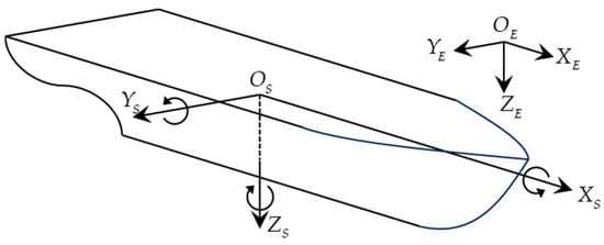
Figure 1.
Geodetic coordinate system and accompanying ship coordinate system.
For a practical application, this paper establishes a resting period standard by referencing the criteria outlined in the official literature cited in the previous section and integrating the standards used by a flight automatic control research institute. Specifically, the resting period is defined as the continuous time from the current moment that meets the following three conditions simultaneously.
(1) Roll: ±2.5°.
(2) Pitch: ±1.5°.
(3) Heave velocity: −2 m/s to 0.5 m/s.
In the previous section, this paper analyzed the prediction durations of resting periods set in various studies and their underlying reasons, considering both the necessary duration for aircraft landing missions and the high accuracy requirements of the predictions. Based on this analysis, this paper selects an 8 s duration from four possible scales: 6–10 s, 8–10 s, 20 s, and 6 s. The chosen duration, which exceeds the necessary landing time of 6 s, ensures that the prediction can be completed within the motion data sampling time used in this study.
The objective of this study is to predict the length of the resting period within the next 8 s to facilitate the safe landing of shipborne helicopters. Therefore, it is necessary to predict the ship’s roll, pitch, and heave over the next 8 s and subsequently calculate the heave velocity. The duration of the time interval that satisfies all conditions within the next 8 s ultimately determines the resting period, which is the focus of this study.
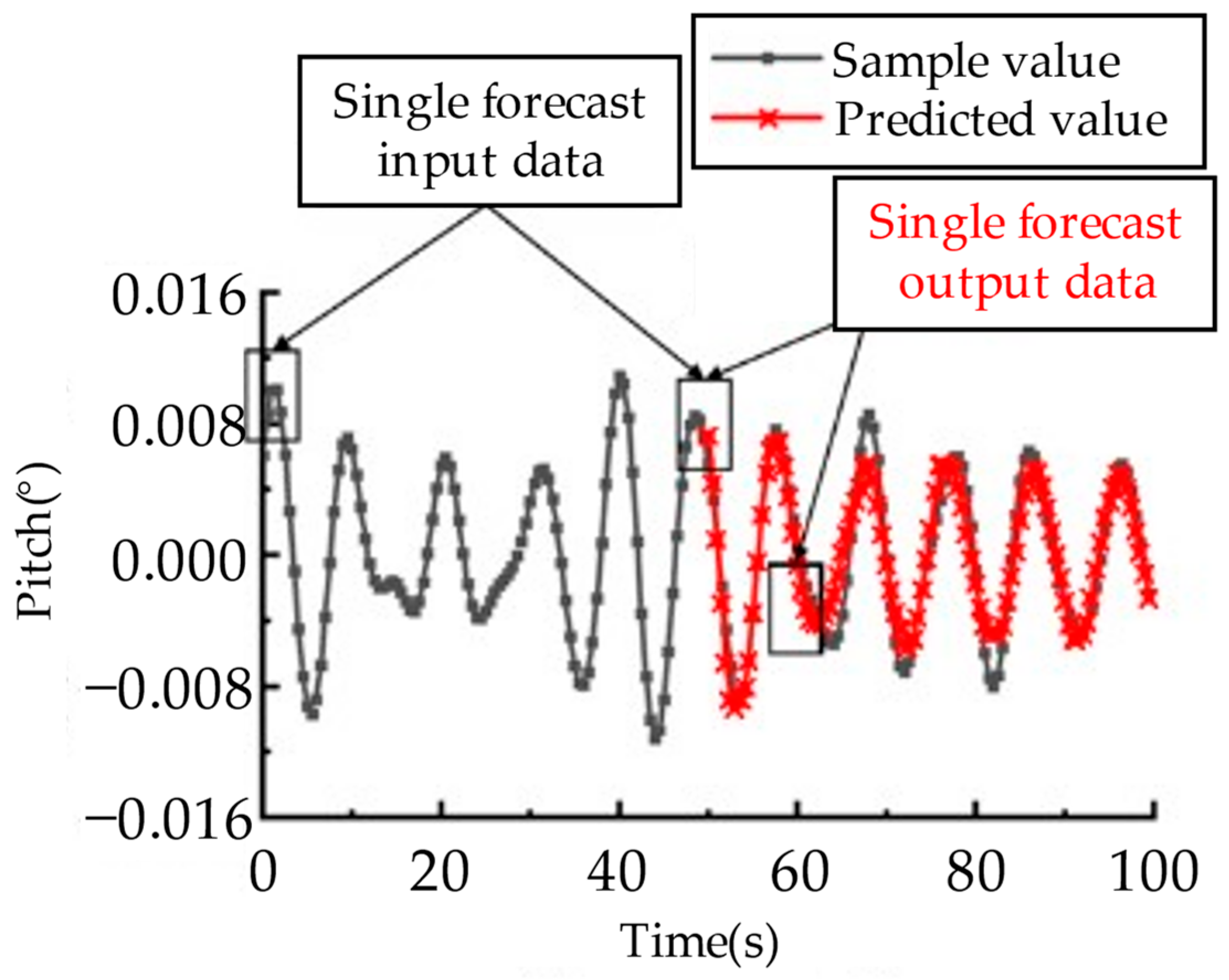
The prediction of the ship motion data can be categorized into single-step and multi-step forecasting. Many existing motion prediction methods primarily focus on single-step forecasting, where input X = {x0, x1, …, xt} represents known data and output Y = {yt+1} is the predicted result. However, this study requires forecasting ship motion data for the next 8 s. Relying solely on a single-step prediction is insufficient for this purpose. Therefore, it is necessary to develop a data prediction model capable of multi-step forecasting, allowing for the prediction of N future steps based on a given length of historical data.
In this study, a direct multi-step output method is employed for prediction, as illustrated in Figure 2. Here, input X = {x1, x2, …, xM−1, xM} is used as the known data, while output Y = {y1, y2, …, yN−1, yN} represents the predicted data. This method is straightforward to implement and can produce multi-step prediction results. However, it disregards the correlations between the predicted values at different future time points. Alternatively, the continuous updating of the latest data for prediction can be performed where the predicted values do not influence subsequent predictions. This approach helps to mitigate issues related to error accumulation and propagation.

Figure 2.
Schematic diagram of direct multi-step output prediction.
To regulate the time steps for prediction and the ratio between the input and output, a time step interval of 0.1 s is used. The input and output data are configured according to a 10:1 ratio. For example, 100 input data points are used to predict 10 target data points, corresponding to using 10 s of known data to predict 1 s of future data. Similarly, 800 input data points predict 80 target data points, corresponding to using 80 s of known data to predict the next 8 s of data. Additionally, careful consideration is given to adjusting the prediction interval and controlling the time consumption of the prediction process to ensure that the trained model can achieve smooth, real-time ship motion response predictions.
In this context, the mapping relationship between the known data and the predicted data established during each prediction step can be approximately represented by the equation y1, y2, …, yN−1, yN = f(x1, x2, …, xM−1, xM, ε). The time-series prediction model constructed in this study is implemented using Long Short-Term Memory (LSTM) networks.
2.2. LSTM Module Building
Long Short-Term Memory Networks (LSTM) represent a specialized form of Recurrent Neural Networks (RNN) specifically designed to learn and retain long-term dependencies. LSTM was first proposed by Hochreiter and Schmidhuber in 1997 [44] and has since been improved and popularized by many researchers. It has demonstrated robust performance across a wide range of applications.
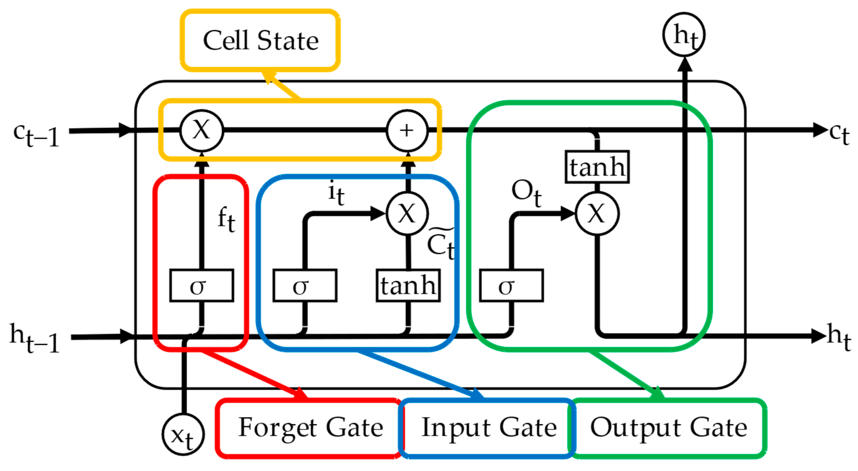
The primary objective of LSTM is to address the challenges associated with long-term dependencies by preserving important information over extended periods, which is crucial for tasks where future outcomes are heavily influenced by past events. Each LSTM unit has a more complex structure than traditional RNN units, as shown in Figure 3.
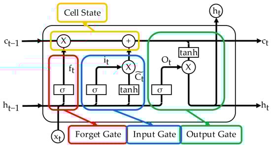
Figure 3.
LSTM neurons.
The key element of LSTM is the cell state and the iterative formula is as follows:
ct = ft ⊙ ct−1 + it ⊙ c~t.
Each LSTM unit performs simple addition and subtraction operations along this pathway, ensuring the preservation of long-term dependency information.
The first step in LSTM operation involves the forget gate, which determines which information to discard from the cell state. The iterative formula is as follows:
where Wf represents the weight of the forget gate connection, bf is the bias of the forget gate, and σ(x) is an activation function. Through the sigmoid function, the values are converted to between 0 and 1, determining how much of the previous cell state is retained.
ft = σ (Wf ∙ [ht−1, xt] + bf),
σ(x) = 1/(1 + e−x),
The second step in LSTM involves the input gate, which governs the storage of new information. The iterative formula is as follows:
where Wi and Wc represent the weights of the input gate and the cell state connection for this calculation; bi and bc are the biases of the input gate and the calculated cell state, respectively; and tanh(x) is another activation function. First, the sigmoid function decides which values to update, and then the tanh function generates candidate values.
it = σ (Wi ∙ [ht−1, xt] + bi),
c~t = tanh(Wc ∙ [ht−1, xt] + bc),
tanh(x) = (ex − e−x)/(ex + e−x),
Finally, the output gate of LSTM determines the output content based on the current cell state. The iterative formula is as follows:
where Wo represents the weight of the output gate connection and bo is the bias of the output gate.
ot = σ (Wo ∙ [ht−1, xt] + bo),
ht = ot ⊙ tanh(ct),
As summarized in the figure, the main transmission pathway in LSTM neurons represents long-term memory, while the lower pathway corresponds to short-term memory, which is why it is named “Long Short-Term Memory.”
Based on the aforementioned LSTM principles, the most critical LSTM component of the prediction model is constructed. A single-variable experiment is conducted to determine the hyperparameters of LSTM. The hyperparameter settings of the LSTM model used in this paper are shown in Table 1.

Table 1.
Hyperparameters of LSTM in this paper.
2.3. Ship Motion Prediction Model Training
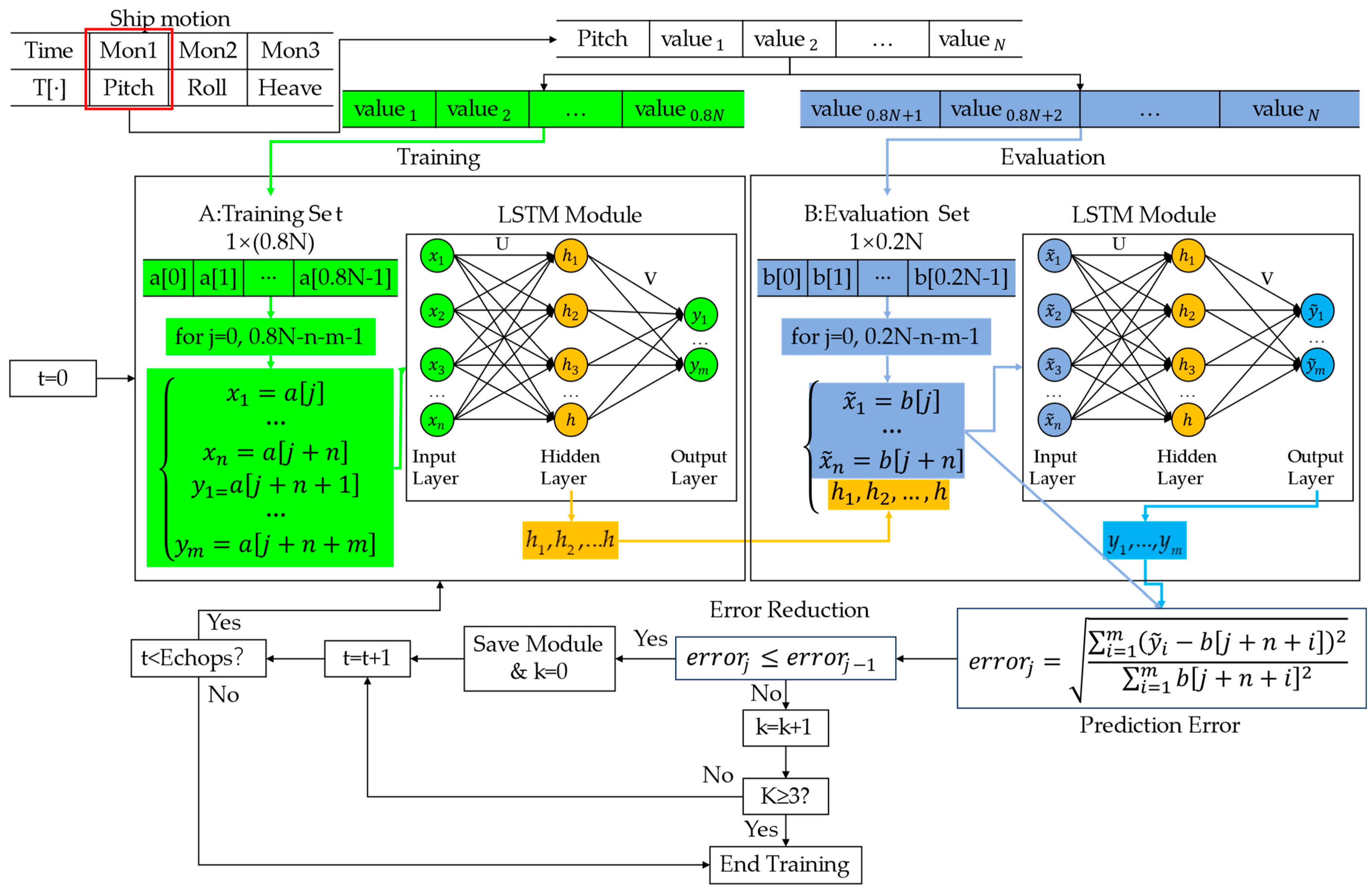
After the LSTM model is constructed, the ship motion prediction model can be developed. The main steps of model training are illustrated in Figure 4.

Figure 4.
Model training process.
Data Reading and Processing: The motion data of the current degree of freedom are read from the data file and imported into the data loader for processing. In this paper, training and prediction are conducted sequentially based on the order of degrees of freedom, with a consistent sampling interval for data points. The current motion data for each degree of freedom are stored in a one-dimensional array, where each position in the array represents the motion data at a specific time-point. Normalization is then performed on the data to enhance the model’s accuracy and computational efficiency. The maximum and minimum normalization method is used to scale the data to the range of 0 to 1. Its formula is as follows:
x’ = (x − mini)/(maxi − mini).
The maximum and minimum values for each degree of freedom in the training set are recorded and saved for future reference.
Following normalization, the dataset is divided into a training set and a testing set, comprising 80% and 20% of the data, respectively. The training set is utilized for model training, while the testing set is employed to evaluate the early stopping mechanism. Finally, both datasets are transformed into the input format required by the Long Short-Term Memory (LSTM) model. In this step, the data, initially received as a one-dimensional array, undergo normalization and other preprocessing to be transformed into input–output pairs. These pairs capture the current sequence and the predicted target sequence at each location. The input–output pairs are generated by sliding a window of a specified length (seq_length) over the time-series data. During each iteration, an input sequence x is created by slicing the data from index i to (i + seq_length). The corresponding target value y is then obtained by selecting the data point at index (i + seq_length). At this stage, the data structure transitions from a list of values to a tensor format.
Prediction Model Construction and Training: The LSTM calling module is written, and the overall structure of LSTM is constructed. Based on the results of preliminary single-variable experiments, the LSTM hyperparameters are set, and the hidden state and cell state are initialized to zero vectors. The LSTM model is trained using the processed training set data. First, the loss function and optimizer are set. Reference [45] thoroughly investigated the existing loss functions in a time-series analysis for regression tasks, and its experiments showed that MAE, MSE, and Huber loss performed well. However, gradients of MAE are large for the small values that ship motion often has, which is not good for learning, and Huber loss is less sensitive than MSE, which may make it difficult to achieve the required training accuracy. In comparison, MSE is the most suitable loss function for this paper. Therefore, the mean square error (MSE) is selected as the loss function to measure the prediction error. And, the Adam optimizer is used to update the model parameters during gradient descent. The MSE formula is as follows:
where ŷi is the predicted values and yi is the actual values.
MSE = Σni=1(ŷi − yi)2/n,
At the end of each training iteration, the model makes predictions on the test set, and the prediction error is calculated according to the following predefined formula. Different from training when input–output pairs are known and model weights are obtained by LSTM modeling, the model inputs are known during testing and the model weights are used to predict the output sequence of each input using the parameters saved during the last precision improvement.
where y* is the predicted values and yi is the actual values. If the prediction error decreases compared to the previous iteration, the current model parameters are saved; otherwise, the best previously saved model parameters are retained. If the prediction error on the test set increases for three consecutive iterations, the early stopping mechanism is triggered, indicating that the model may be overfitting. In such cases, the training process for the current degree of freedom is terminated. If the early stopping mechanism is not triggered, the model continues to train until the maximum number of iterations (epochs) is reached.
error = (Σn1(yi − y*)2/Σn1 yi2)1/2,
Post-training Process: Upon the completion of the training process, the final model parameters are saved to a file, and the model is used to make predictions on the training set. The predicted results and the actual values from the training set are stored together in the prediction comparison array for the current degree of freedom. After completing these steps, the training for one degree of freedom is finalized. The training process for the next degree of freedom then begins, repeating the same steps. Once training is complete for all degrees of freedom, the predicted values and actual data for each degree of freedom are saved together in a file for subsequent viewing and analysis. During the prediction loop, the trained model can be loaded by reading the model parameter file corresponding to each degree of freedom.
3. Experiment
3.1. Engineering Scenario
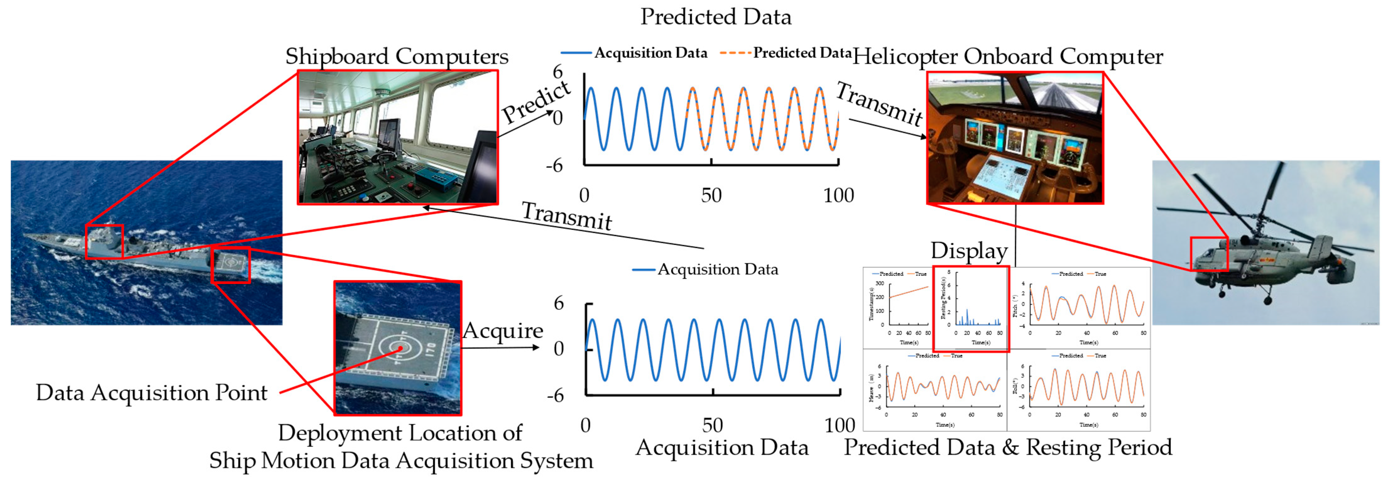
The objective of this study is to predict the ship motion resting periods in a practical engineering context by developing a prediction model and establishing information transmission channels across multiple devices, thereby facilitating the safe landing of shipborne helicopters on the ship’s deck. The engineering scenario is depicted in Figure 5.
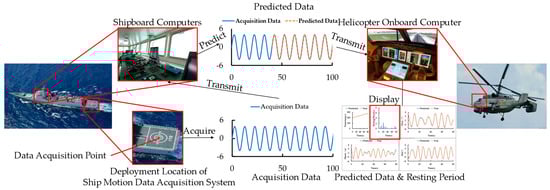
Figure 5.
The actual engineering scenario simulated in this paper.
First, the ship’s motion data acquisition system is responsible for measuring and recording the ship’s motion data. This system is installed in the helicopter landing area on the ship’s deck to capture real-time six-degrees-of-freedom motion data for the area and to record these data as a time-series. Since the helicopter landing area can be regarded as a rigid plane, the roll and pitch angles at various points within the area can be considered identical with minimal variation. Meanwhile, the heave velocity at a point can be calculated using the following formulas:
where cp and ċp represent the heave and heave velocity at a given point; c, α, and β denote the heave, roll, and pitch of the ship’s center of gravity, respectively; ċ, αt, and βt represent the heave velocity, roll angular velocity, and pitch angular velocity of the ship’s center of gravity, respectively; and xg and yg are the horizontal and vertical coordinates of the ship’s center of gravity.
cp = c − (x − xg)sinβ + (y − yg)sinα,
ċp = ċ − (x − xg)βtcosβ + (y − yg)αtcosα,
Since the actual contact point during the helicopter landing is the landing gear, which has a small contact area, and the displacement and velocity of the three relevant degrees of freedom are low during the resting period, the motion data collected at the center of the landing pad can effectively represent the motion of the entire pad.
The ship motion data acquisition system transmits the collected data to the onboard computer. So, a data transmission channel between the ship motion data acquisition system and the onboard computer is established, typically via wired or wireless means.
Upon receiving the data, the onboard computer uses the motion data to train the prediction model. The necessary software and hardware are installed on the onboard computer, which then executes the training module to develop the prediction model. The accumulated ship measurement dataset is used during training to adapt the model to the current sea conditions. To ensure that the prediction model continuously adapts to changing sea conditions, the model training module should operate continuously, updating the model parameters based on the latest data to maintain the prediction accuracy.
Subsequently, the onboard computer employs the trained prediction model to predict the ship’s future motion data and resting period in real time. The system can perform real-time online predictions and provide critical resting period information using the most recent model parameters. To ensure the efficiency of the data transmission and program operation, the prediction model’s computational efficiency must be high enough to meet the data transmission interval requirement of 0.1 s. By predicting the ship’s motion data for the next 8 s, the length of the ship’s resting period can be determined. Since the accurate prediction of the ship’s motion data is essential for determining the resting period, the prediction model must exhibit exceptionally high accuracy.
During the prediction process, the onboard computer transmits the future motion data and resting period information to the shipborne helicopter’s onboard computer. The primary goal of the prediction is to determine the resting period length for the next 8 s, assisting the pilot in identifying the optimal landing time and ensuring higher safety and success rates. Therefore, the prediction results must be transmitted and displayed immediately to the helicopter’s onboard computer. Given that only the resting period within the next 8 s is predicted, minimizing transmission time enhances the effectiveness of the prediction results. Thus, high-speed wireless transmission is recommended.
Based on the ship’s motion data and resting period information displayed on the onboard computer, the pilot selects the appropriate landing time and completes the landing. With the assistance of the resting period information, the pilot can significantly reduce the cognitive load during landing, thereby improving the landing efficiency and safety.
Since the model proposed in this study is still under development, it is not yet suitable for large-scale, long-duration, and high-risk field experiments involving actual ships and helicopters. Therefore, this study employs multiple devices for simulation experiments to validate the model’s applicability in real-world engineering scenarios.
3.2. Experimental Data Set
The data used in this paper were obtained by desensitizing data collected on real ships by a flight automatic control research institute. Due to confidentiality concerns, specific details about the ships, helicopters, and data acquisition methods cannot be disclosed. As indicated in Table 2, the experiment involved data from three different ship types, two speeds, and four sea states.
Table 2.
Information on each experimental condition.
For each condition, motion data were collected over a period exceeding 2000 s, with a data collection interval of 0.05 s. The data were then split into a training set and a prediction set in a 4:1 ratio. Specifically, the training set spans 1600 s, comprising 32,000 data points, while the prediction set covers 400 s, consisting of 8000 data points. To simulate real-world conditions more accurately, the motion data transmission system in the subsequent simulation will also transmit data at 0.05 s intervals.
3.3. Experimental Procedure
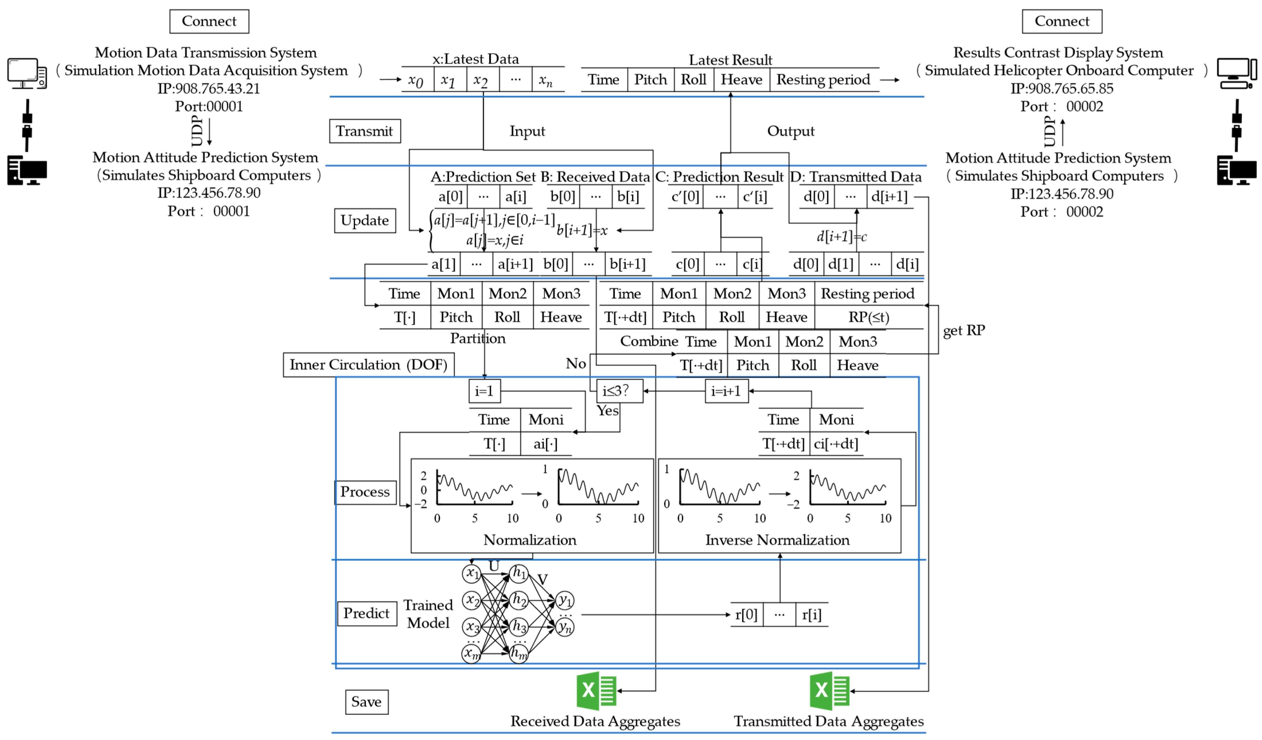
The prediction model developed in this study enables real-time online forecasting, as depicted in Figure 6, by continuously receiving the latest data and generating immediate prediction results. The entire process involves three devices: a motion data transmission system simulating the ship’s motion acquisition system, a motion prediction system simulating the ship’s onboard computer, and a result comparison and display system simulating the onboard computer of the shipborne helicopter.
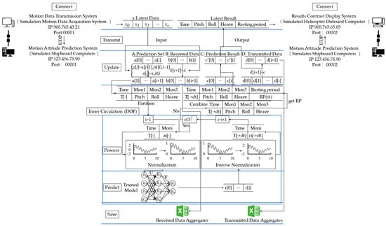
Figure 6.
Real-time online prediction.
The overall prediction process consists of the following steps (Algorithm 1):
| Algorithm 1: Predict with our proposed Motion Prediction System |
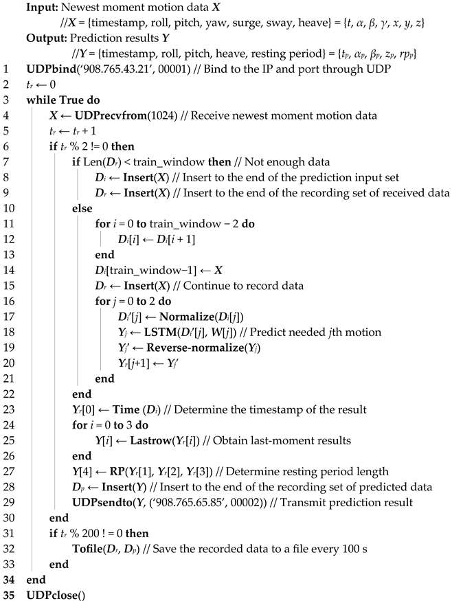 |
(1) UDP Protocol Setup and Information Reception: The UDP protocol is established between the motion data transmission system and the motion prediction system. The motion data transmission system simulates the ship motion acquisition system, sending the latest data array—including the time, roll, pitch, surge, sway, and heave data— to the IP address and designated port of the motion prediction system every 0.05 s. To allow sufficient time for the prediction and data transmission process, the motion prediction system receives the latest data every 0.1 s, which means it only receives one set of data for every two sets sent by the motion data transmission system. After receiving the latest data, the system decodes it, converting the received data format into the format required for subsequent operations.
(2) Data Update and Accumulation: Predicting the length of the resting period within the next 8 s requires forecasting the ship’s motion data for the next 8 s. The motion prediction system continuously receives data from the motion data transmission system. When the accumulated data span is less than 80 s, the latest data are continuously appended to the end of both the prediction set and the received data set. When the accumulated data span exceeds 80 s, only the latest 80 s of data are retained in the prediction set, while the received data set continues to add the latest data to maintain a record of all the actual data received by the motion prediction system.
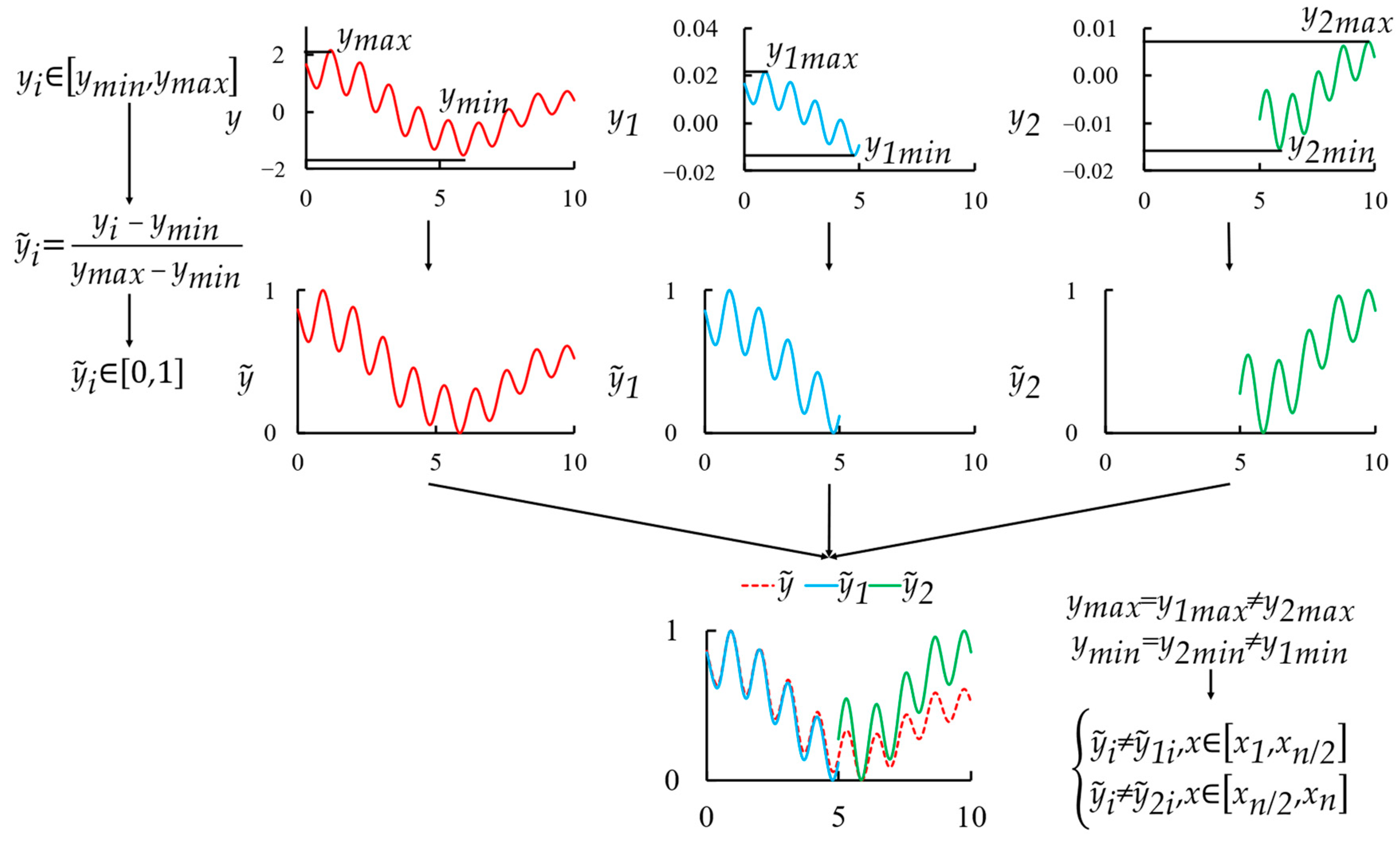
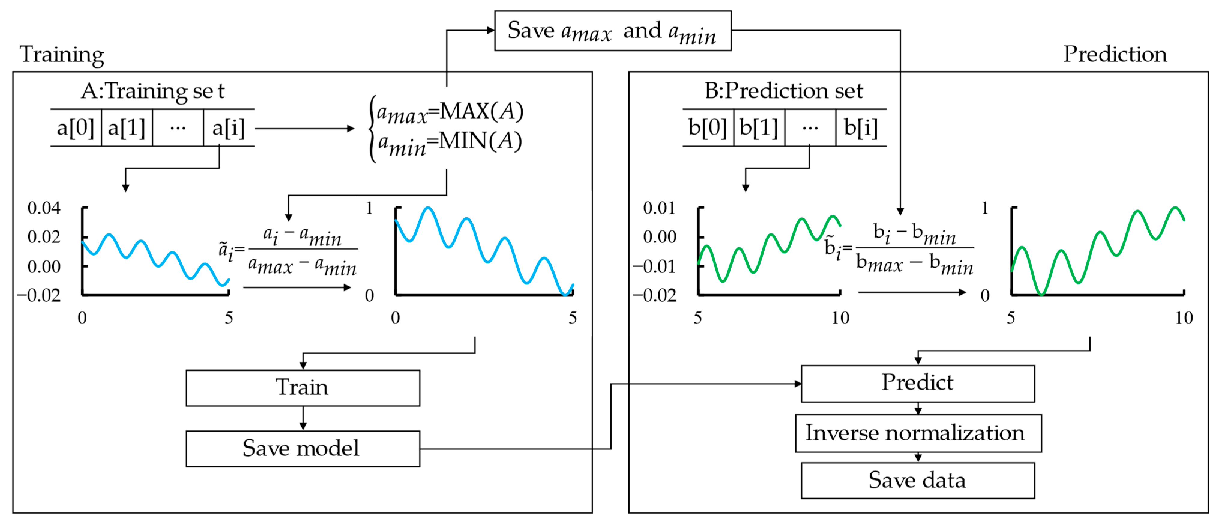
(3) Data Segmentation and Processing: Once the accumulated data span in the prediction set exceeds 80 s, data segmentation begins. The data are first divided into “time-current degree of freedom data” pairs according to their respective degrees of freedom. The data loader then reads the maximum and minimum values of the training set’s current degree of freedom motion data recorded during training. These values are used to normalize the prediction set data and convert the data format to the format required for LSTM operations. Using the maximum and minimum values of the training set for normalization during prediction is necessary because a real-time online prediction cannot access all motion data. If the data are processed according to the current test set’s extreme values for each prediction, a numerical offset may occur, as shown in Figure 7. Therefore, the training set’s extreme values, as illustrated in Figure 8, are used as the standard for data processing during prediction.
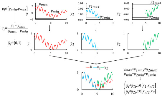
Figure 7.
Numerical offset in normalization.
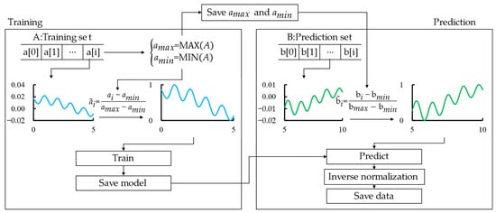
Figure 8.
Prediction set normalization.
(4) Motion Data Prediction: Similar to the training process, the LSTM module is implemented, the overall structure of the LSTM network is constructed, and the hyperparameters are set. Before prediction, the hidden state and cell state are initialized to zero vectors. The model parameters file obtained during training is loaded and the model is imported to update the prediction models for each degree of freedom motion. After the prediction, the data are normalized back to their original range, as the predicted results are also within the 0 to 1 range. After predicting the motion data for each degree of freedom, the length of the resting period within the next 8 s is determined based on the ship’s roll, pitch, and heave velocities (the heave velocity is obtained by dividing the difference between adjacent heave results by the time interval of 0.1 s). All results are combined into a five-column dataset in the order of “time-roll-pitch-heave-resting period length,” and the last row of the dataset is recorded in both the prediction result set and the transmission data set.
(5) Motion Data Transmission and Display: A data transmission channel is also established using the UDP protocol between the result comparison and display system and the motion prediction system. After each prediction based on the latest data, the motion prediction system encrypts the data in the prediction result set and sends it to the result comparison and display system simulating the shipborne helicopter’s onboard computer. The results comparison and display system synchronously displays all the data used for the prediction and provides a real-time rolling display of the data transmitted by the motion data transmission system. As shown in Figure 9, after receiving the data sent by the motion prediction system, the result comparison and display system compares the latest predicted results with the actual values at the corresponding time and displays the resting period length for the next 8 s in real-time.
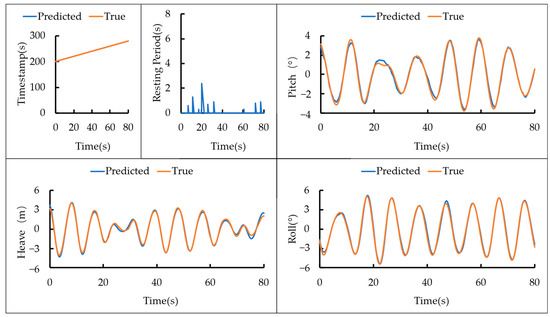
Figure 9.
Results display and comparison.
The first sub-window in the top row of the interface displays timestamps for both the predicted and actual values, allowing for a comparison to identify any transmission delays. The second sub-window in this row shows the predicted duration of the ship’s resting period over the next 8 s, based on the three degrees of freedom motion and the resting period criteria used in this study. The rightmost sub-window in the top row compares the actual pitch to the predicted pitch. The sub-windows in the second row present comparisons of the true and predicted values for heave and roll, respectively. The interface updates in real-time with new data every 0.1 s, causing the curves to shift 0.1 s to the left on the axis. The horizontal axis in each sub-window spans 80 s, corresponding to the time span of the LSTM model’s input sequence used in this study.
After completing the above steps, one data reception and prediction process is finished. This process typically completes all data transmissions and predictions within 0.1 s. Therefore, the motion prediction system can receive the latest set of data 0.1 s later and start a new prediction process for the next moment, continuously advancing the loop. Additionally, the motion prediction system periodically saves the total received data set and the total transmission data set to two sheets in an Excel file for later review. If the entire process needs to be terminated, data transmission is stopped in the motion data transmission system. The program is then terminated in the motion prediction system and the data reception is halted in the result comparison and display system, thereby ending the operation of all systems.
4. Results
To ensure the representativeness of the real-time online prediction experiment results, this study utilized actual measurement data collected from real ships. The experimental conditions include three distinct vessels, encompassing motion data at various speeds and under different sea states. It is noteworthy that under certain low-wave-height conditions, the ship’s motion amplitude and rate of change fall within the criteria for a resting period, indicating that the ship is in a resting period throughout the experiment. Such conditions are not conducive to thoroughly testing the model’s ability to predict future resting periods, and thus, these non-representative conditions were excluded from the analysis.
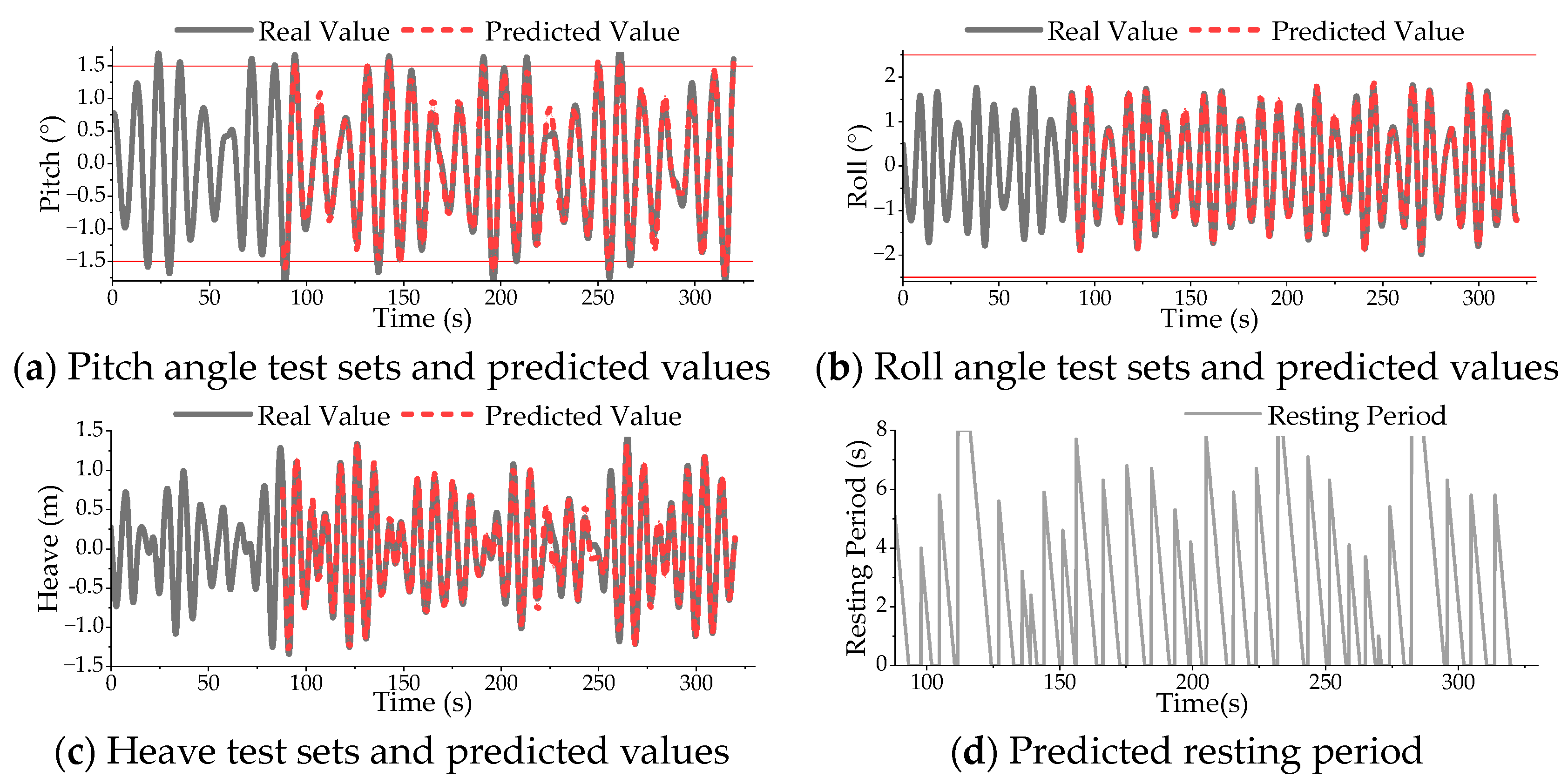
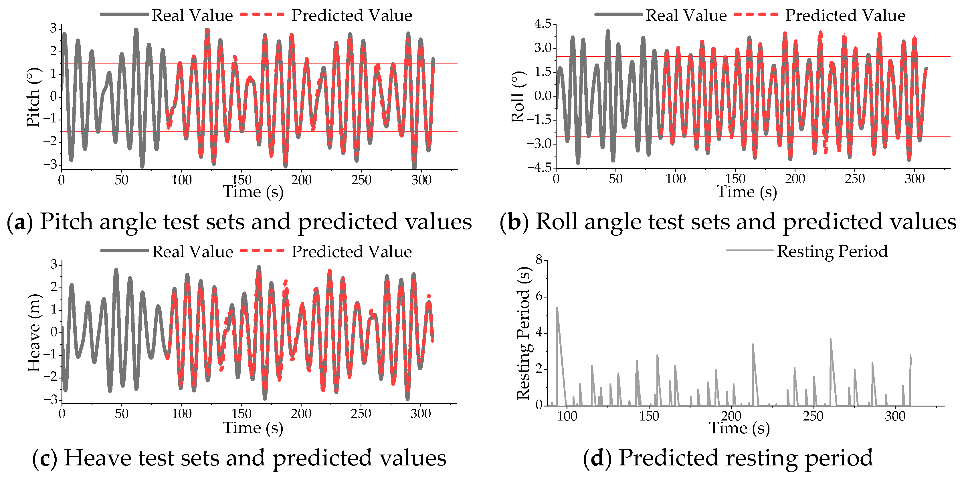
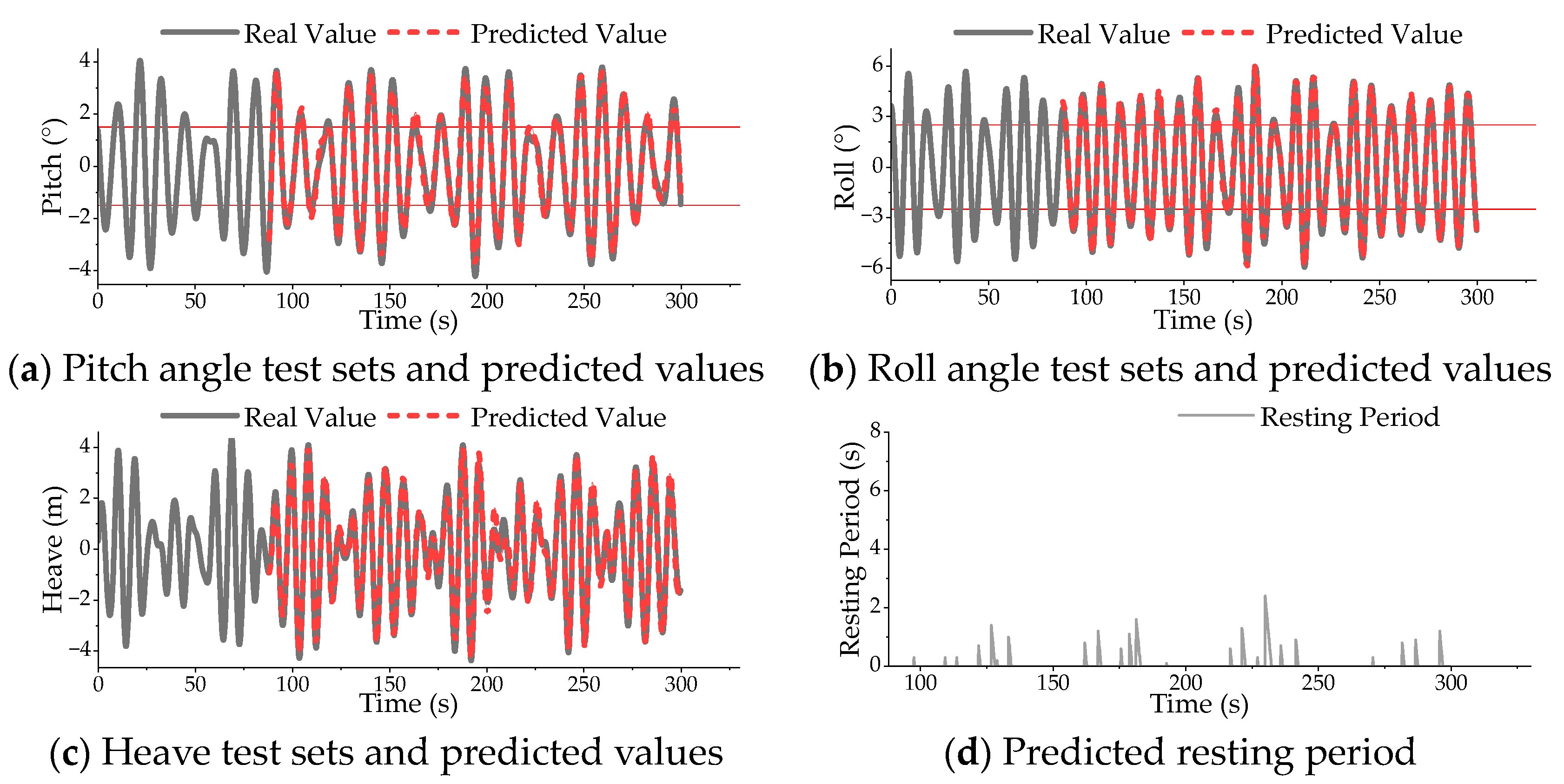
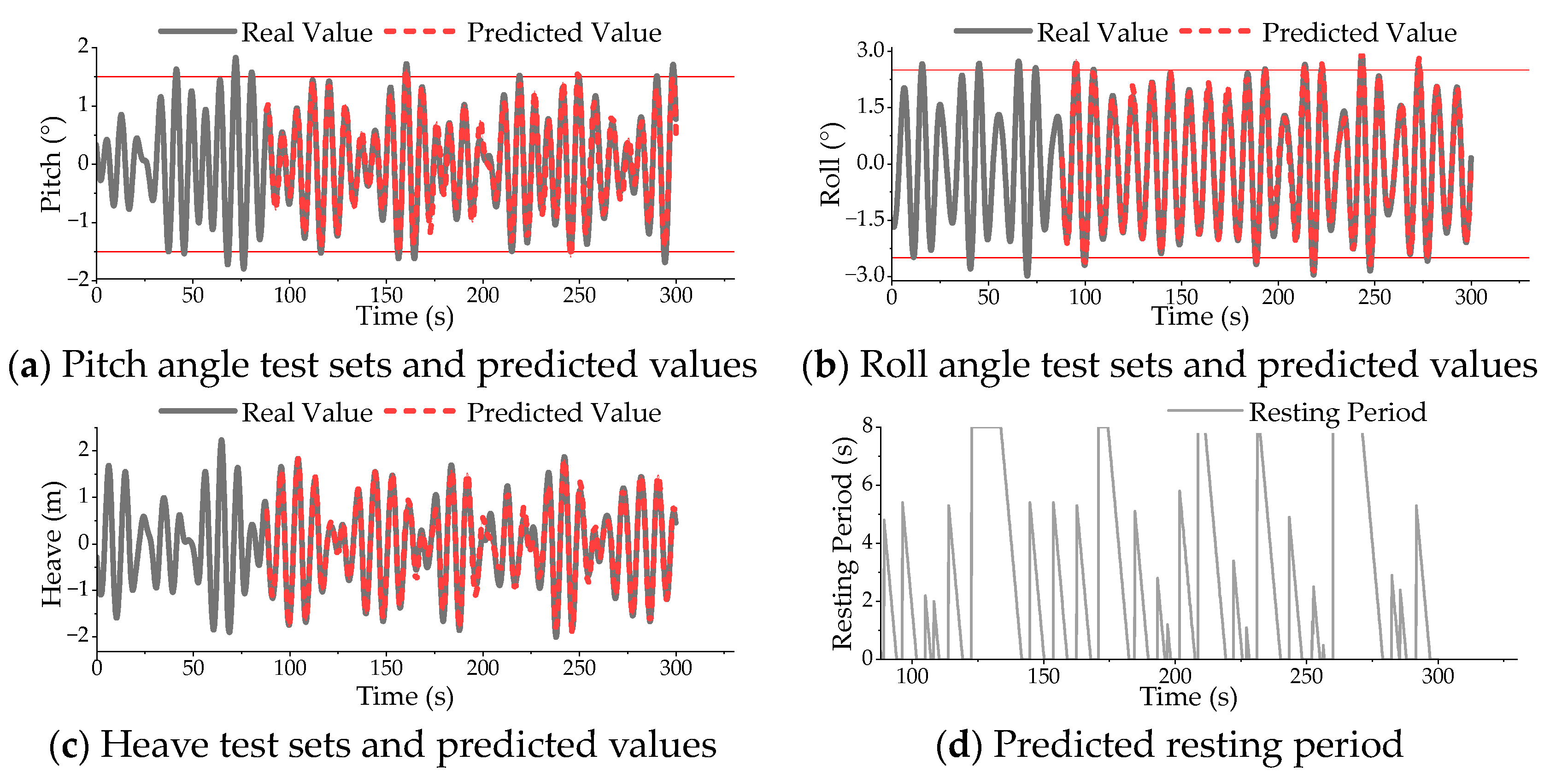
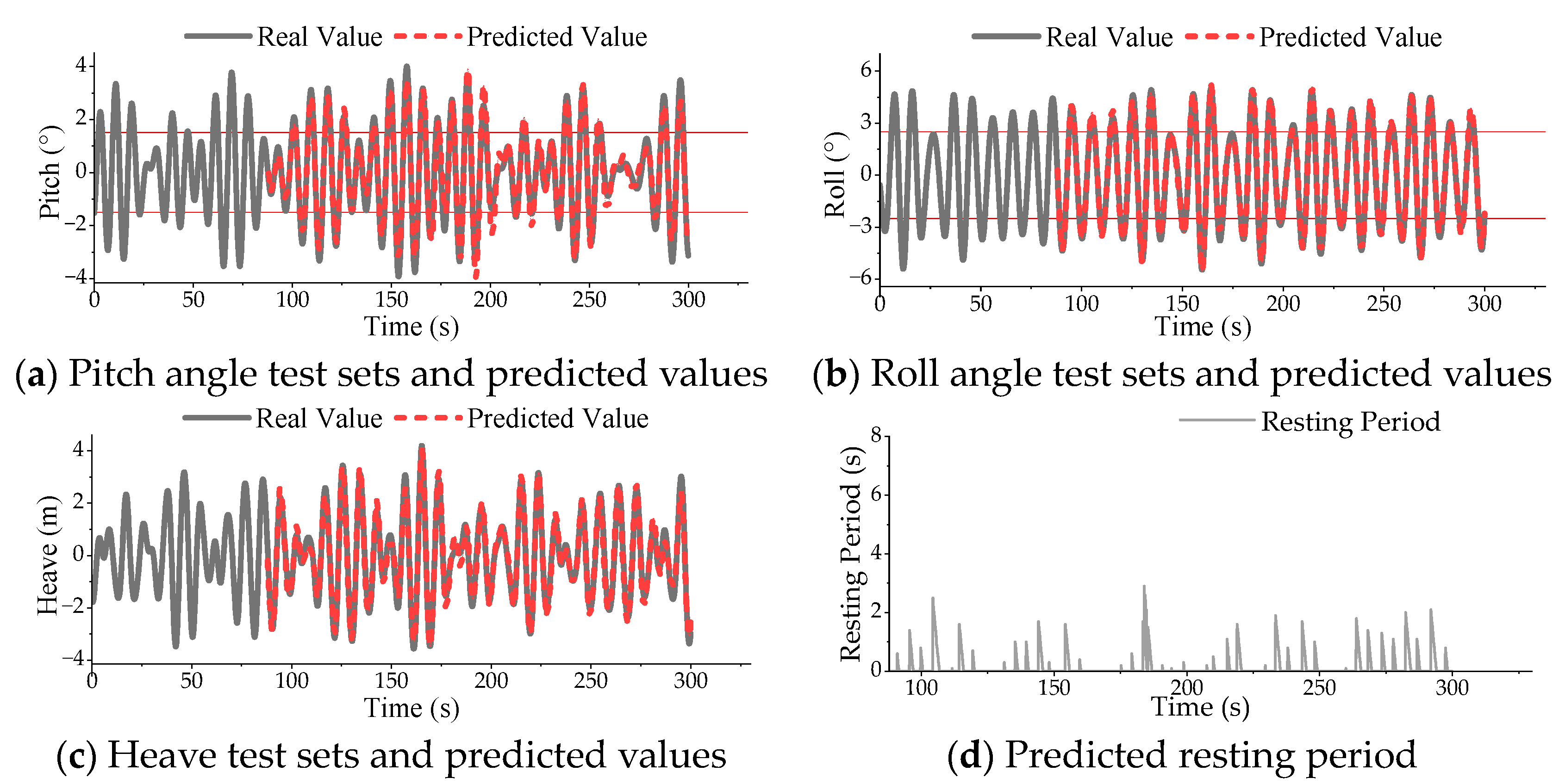
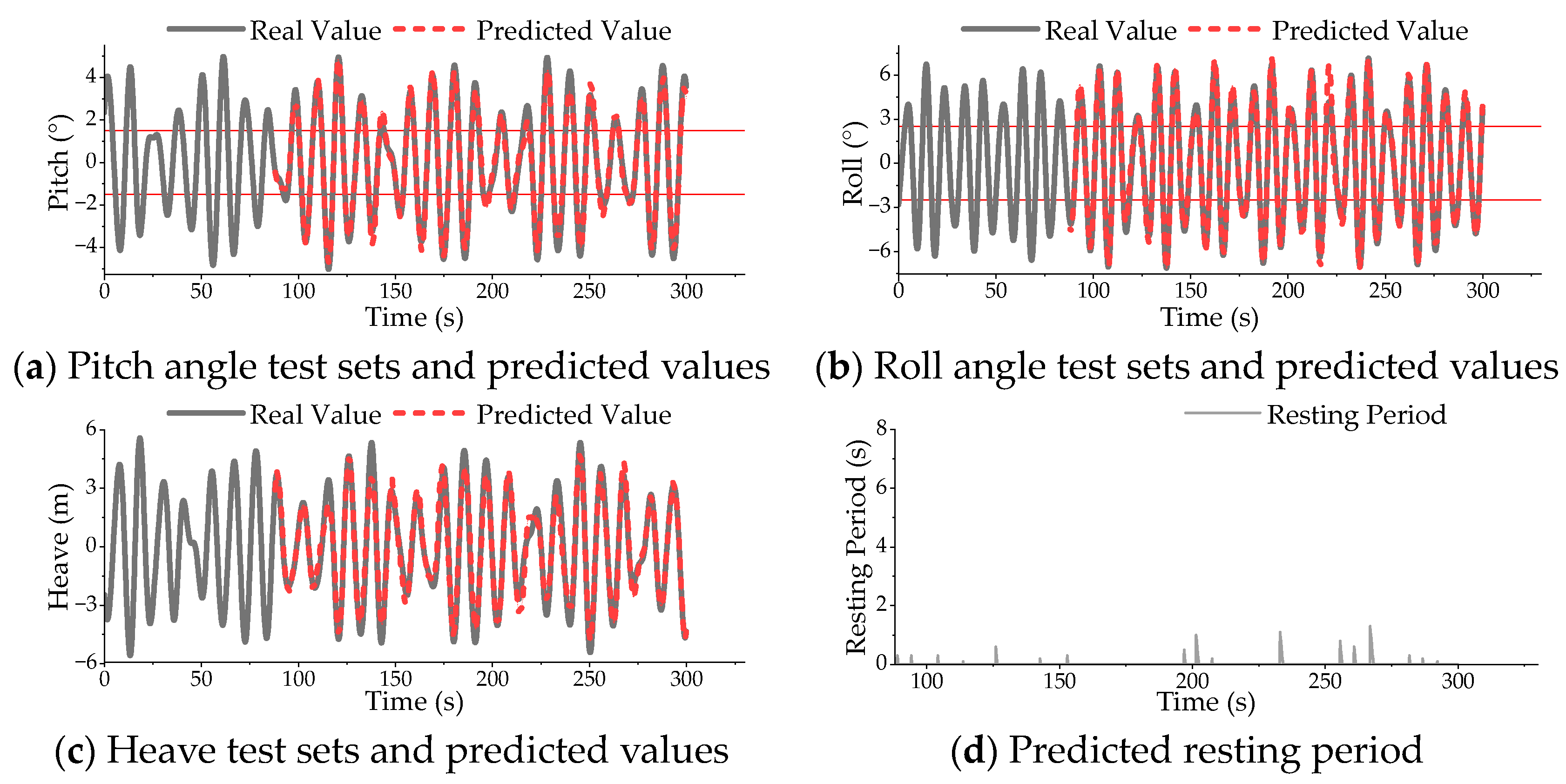
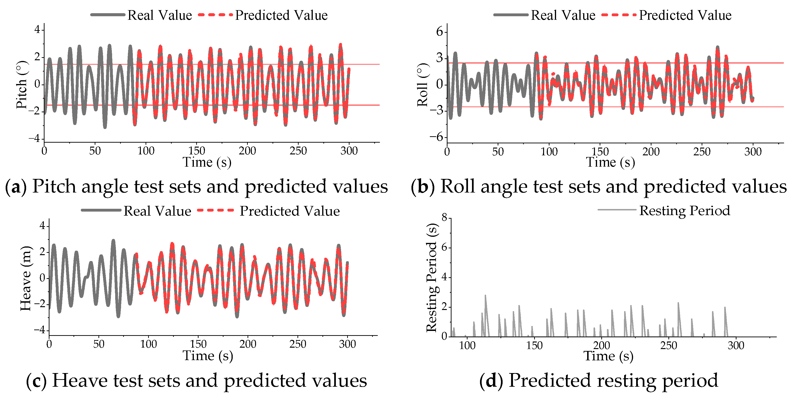
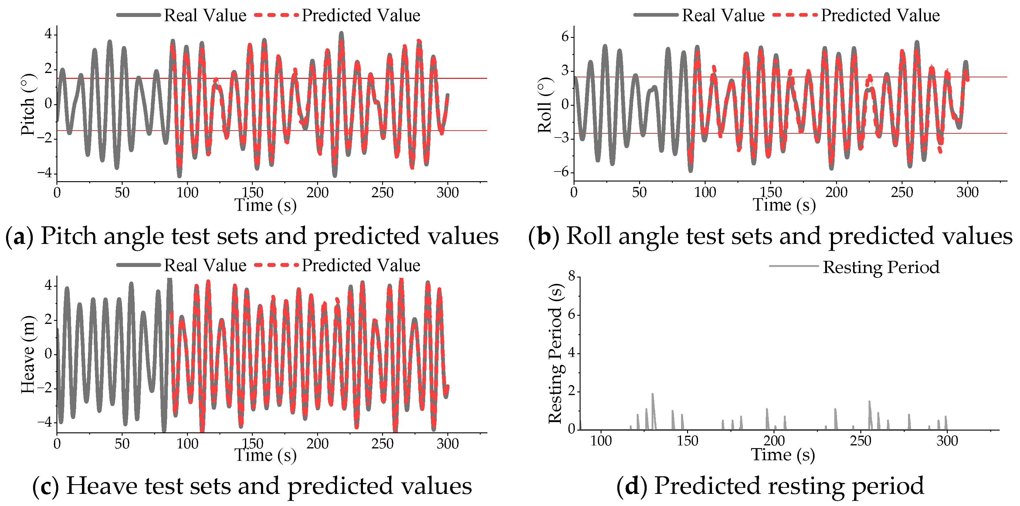
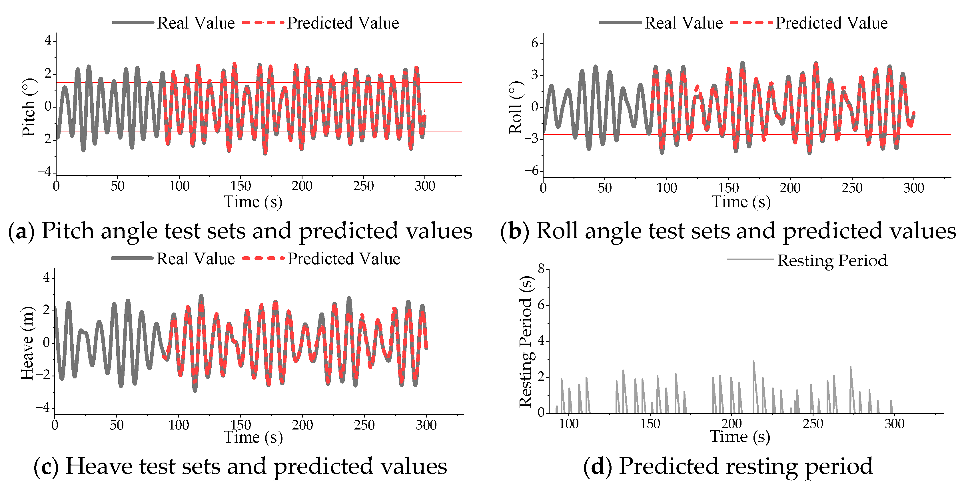
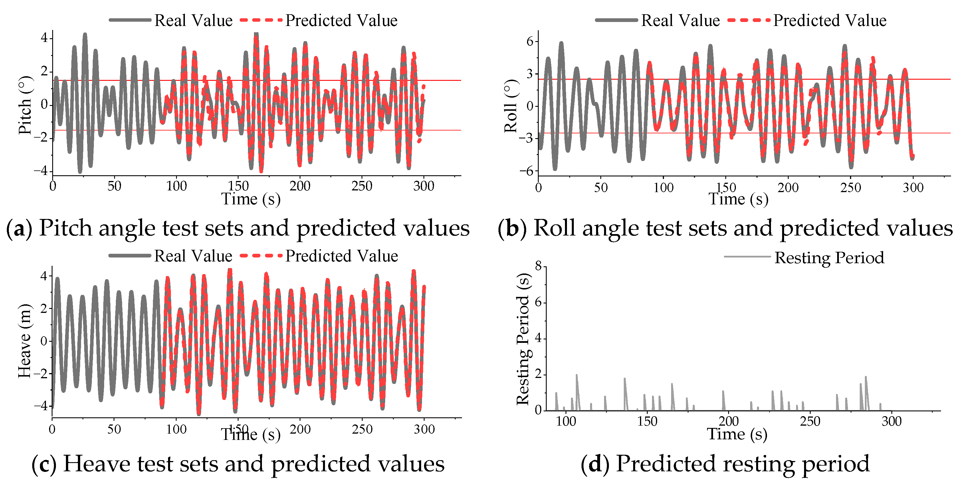
Data from ten randomly selected conditions were drawn from a larger dataset of actual measurements. These conditions were explicitly chosen to effectively validate the prediction accuracy of the proposed model. The specific experimental results are presented in Figure 10, Figure 11, Figure 12, Figure 13, Figure 14, Figure 15, Figure 16, Figure 17, Figure 18 and Figure 19, where each condition’s results include four subplots: subplot (a) compares the pitch angle test set with the predicted values; subplot (b) compares the roll angle test set with the predicted values; subplot (c) compares the heave test set with the predicted values; and subplot (d) depicts the predicted length of the ship’s resting period for the next eight seconds based on the data from the three degrees of freedom, with a maximum prediction horizon of 8 s.
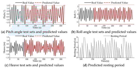
Figure 10.
Condition 1 data comparison.

Figure 11.
Condition 2 data comparison.

Figure 12.
Condition 3 data comparison.
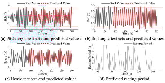
Figure 13.
Condition 4 data comparison.
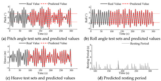
Figure 14.
Condition 5 data comparison.
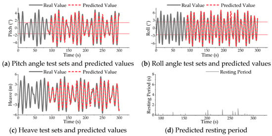
Figure 15.
Condition 6 data comparison.
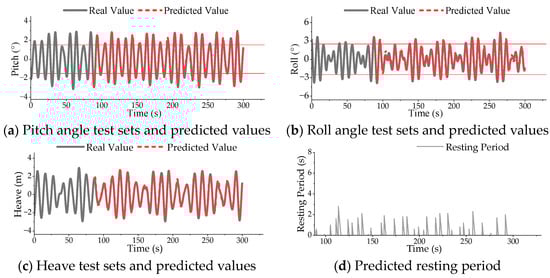
Figure 16.
Condition 7 data comparison.
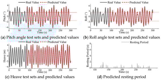
Figure 17.
Condition 8 data comparison.
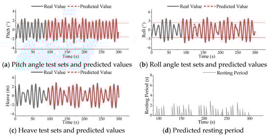
Figure 18.
Condition 9 data comparison.

Figure 19.
Condition 10 data comparison.
To visually represent the impact of pitch and roll on the ship’s resting period, two lines parallel to the horizontal axis are drawn in subplots (a) and (b) of each condition, indicating the motion range that meets the resting period criteria. As shown in the figures, the LSTM model exhibited strong predictive accuracy, with the predicted values closely aligning with the actual data across all tested conditions.
Through multiple predictions using real-world data, it was observed that the model’s predictions were generally close to the actual data, particularly under relatively stable operating conditions. An analysis of the motion data across the three degrees of freedom and the results during rest periods reveals that pitch, roll, and heave directly influence the prediction of the rest period duration. When the pitch and roll angles are small, the vessel’s motion tends to stabilize, facilitating the formation of longer rest periods. The variation in the heave speed also significantly impacts the rest period; when the speed fluctuates within an acceptable range, the rest period can be maintained.
If the pitch, roll angles, and heave speed simultaneously meet the criteria for defining a rest period, the onset of the rest period can be identified. However, as time progresses, fluctuations in the data for these three degrees of freedom will affect the duration of the rest period. The rest period ends when any parameter in one of the degrees of freedom exceeds the specified range.
The prediction accuracy of the model was calculated using the error formula presented earlier in Formula (11). The prediction errors between the predicted values and the actual values for the three degrees of freedom under each condition were calculated based on the received and transmitted data stored in the program. The results are summarized in Table 3.
Table 3.
Online real-time prediction error of each experimental condition.
As shown in the table, the prediction error for the three degrees of freedom motion data is within 15%, with a maximum error of 14.97%. Given that the error remains within a small range, the predicted ship motion resting period based on these degrees of freedom demonstrates high reliability.
The experimental results confirm that the proposed model can accurately predict the length of the resting period, validating its effectiveness and feasibility in practical applications.
The findings indicate that the proposed method maintains high prediction accuracy across various conditions, with a maximum error of less than 15%. This level of accuracy meets the requirements for providing auxiliary information for helicopter landings on ships. In most cases, the predicted results closely align with actual data, demonstrating the effectiveness of deep learning techniques, particularly LSTM models, in handling complex nonlinear time-series data and their suitability for ship motion and resting period prediction.
5. Discussion
This study explores the use of an LSTM-based method for predicting ship motion across multiple degrees of freedom and proposes a high-precision real-time online prediction model for determining resting periods. The effectiveness and feasibility of predicting ship resting periods by forecasting the pitch, roll, and heave motions were validated through experimental analysis using actual measured data.
The experimental results demonstrate that the proposed method maintains a maximum prediction error within 15% under various conditions, indicating a high level of accuracy that meets the requirements for providing auxiliary information for shipborne helicopter landings. In most scenarios, the predicted results closely align with the actual data, confirming that deep learning techniques, particularly LSTM models, are effective in handling complex nonlinear time-series data and are well-suited for predicting ship motion and resting periods.
The comparison of resting period predictions under different operating conditions reveals key insights. For the same ship type, when sailing at a constant speed across varying sea states, an increase in the sea state level leads to a decrease in both the frequency and duration of the ship’s resting period. Similarly, when comparing different speeds under identical sea states, higher speeds result in shorter resting periods in terms of both the frequency and duration. Moreover, variations in the ship type, even under identical environmental conditions, can lead to differences in the resting period characteristics. Therefore, to achieve longer resting periods, it is advisable to reduce the speed and navigate in areas with lower sea states.
The prediction error analysis reveals that the model used in this study exhibits smaller errors when predicting the Roll and larger errors when predicting the Heave. This discrepancy arises because the model, designed to maintain accuracy while completing the overall process, employs the same framework for predicting all three degrees of freedom: pitch, roll, and heave. However, these motions have inherently different dynamics and behaviors, which means that a uniform predictive model may not capture each motion with equal accuracy. To address this, it is recommended to process the data more carefully to enhance the prediction accuracy without significantly increasing the computational time. Additionally, adjusting the prediction models for each degree of freedom based on their specific characteristics could further improve the accuracy. By tailoring the model to better account for the unique aspects of pitch, roll, and heave, the overall performance of the prediction system could be enhanced, leading to more reliable and precise outcomes in practical applications.
In marine engineering, a trade-off often exists between the real-time performance and prediction accuracy. This study shows that employing LSTM models in conjunction with the UDP transmission protocol enables predictions and data transmission to be completed swiftly, thereby satisfying the real-time performance requirements of practical engineering applications.
Resting periods are a critical factor affecting the safety of shipborne helicopter landings. By accurately predicting the ship’s motion in three critical degrees of freedom, this study successfully forecasts resting period durations. This achievement is significant for enhancing the safety of helicopter operations on ships in complex sea conditions and underscores the broad application potential of resting period prediction in marine engineering.
The model’s short-term prediction capabilities under different sea conditions exhibit strong robustness, especially in stable conditions, where it can accurately determine the length of the resting period, providing reliable support for helicopter landings. However, under conditions with rapid changes in motion, the model’s prediction accuracy declines, suggesting that future research should focus on enhancing the model’s adaptability to complex sea conditions. Specifically, considerations should be given to improving the model’s scalability and adaptability to ensure consistent prediction accuracy across various sea conditions.
Future research will focus on the three main directions: first, further optimizing the LSTM model structure to improve the prediction accuracy under rapidly changing conditions; second, exploring multi-model fusion techniques by integrating other machine learning or physical models to enhance the model’s applicability in complex sea conditions; and third, optimizing data transmission and processing mechanisms to ensure that the model maintains a high prediction accuracy under more stringent real-time requirements.
6. Conclusions
This paper presents a method for predicting ship motion across multiple degrees of freedom and resting periods using LSTM, which was validated through experimental analysis. The application of this method in practical engineering demonstrates its strong applicability and feasibility, providing robust support for the safe landing of shipborne helicopters and suggesting directions for future research.
In summary, the findings of this study offer substantial technical support for practical applications in the field of ship and marine engineering and provide valuable insights for future research endeavors. These conclusions not only enrich theoretical research in this field, but also offer practical guidance for engineering practice.
Author Contributions
Conceptualization, Z.C. and X.L.; methodology, Z.C. and X.L.; software, X.L.; validation, X.L. and X.J.; formal analysis, Z.C. and H.G.; investigation, Z.C. and X.J.; resources, Z.C. and H.G.; data curation, Z.C. and X.L.; writing—original draft preparation, X.L.; writing—review and editing, Z.C. and X.L.; visualization, X.L.; supervision, Z.C. and X.J.; project administration, Z.C. and H.G.; funding acquisition, Z.C. and H.G. All authors have read and agreed to the published version of the manuscript.
Funding
This research was funded by the State Key Laboratory of Structural Analysis, Optimization, and CAE Software for Industrial Equipment, Dalian University of Technology, grant number GZ23112, and the APC was funded by the Harbin Institute of Technology at Weihai.
Institutional Review Board Statement
Not applicable.
Informed Consent Statement
Not applicable.
Data Availability Statement
All data, models, or code generated or used during the study are available from the corresponding author by request.
Conflicts of Interest
The authors declare that they have no conflicts of interest in this work.
References
- Geng, L.; Zhang, Y.F.; Wang, J.J.; Fuh, J.Y.; Teo, S.H. Mission planning of autonomous UAVs for urban surveillance with evolutionary algorithms. In Proceedings of the 2013 10th IEEE International Conference on Control and Automation (ICCA), Hangzhou, China, 12–14 June 2013; IEEE: New York, NY, USA, 2013; pp. 828–833. [Google Scholar]
- Waharte, S.; Trigoni, N. Supporting search and rescue operations with UAVs. In Proceedings of the 2010 International Conference on Emerging Security Technologies, Canterbury, UK, 6–7 September 2010; IEEE: New York, NY, USA, 2010; pp. 142–147. [Google Scholar]
- Zhao, D.; Yang, H.; Giuseppe, C.; Li, W.; Ni, T.; Yao, S. Modeling and analysis of landing collision dynamics for a shipborne helicopter. Front. Mech. Eng. 2021, 16, 151–162. [Google Scholar] [CrossRef]
- Memon, W.A.; Ieuan, O.; Mark, D.W. Motion fidelity requirements for helicopter–ship operations in maritime rotorcraft flight simulators. J. Aircr. 2019, 56, 2189–2209. [Google Scholar] [CrossRef]
- Gautam, A.; Sujit, P.B.; Saripalli, S. A survey of autonomous landing techniques for UAVs. In Proceedings of the 2014 International Conference on Unmanned Aircraft Systems (ICUAS), Orlando, FL, USA, 27–30 May 2014; IEEE: New York, NY, USA, 2014; pp. 1210–1218. [Google Scholar]
- Scherer, S.; Chamberlain, L.; Singh, S. First Results in Autonomous Landing and Obstacle Avoidance by a Full Scale Helicopter. In Proceedings of the IEEE International Conference on Robotics and Automation, Piscataway, NJ, USA, 14–18 May 2012; IEEE: New York, NY, USA, 2012; pp. 951–956. [Google Scholar] [CrossRef]
- Scherer, S.; Chamberlain, L.; Singh, S. Autonomous Landing at Unprepared Sites by a Full Scale Helicopter. J. Robot. Auton. Syst. 2012, 60, 1545–1562. [Google Scholar] [CrossRef]
- Zhao, D.; Mishra, S.; Gandhi, F. Real–Time Path Planning for Time–Optimal Helicopter Shipboard Landing via Trajectory Parametrization. Center for Mobility with Vertical Lift Rensselaer Polytechnic Institute: Troy, NY, USA, 2019; unpublished manuscript. [Google Scholar]
- Zhao, D.; Krishnamurthi, J.; Mishra, S.; Gandhi, F. A trajectory generation method for time–optimal helicopter shipboard landing. In Proceedings of the 2018 Annual Forum Proceedings—AHS International, Phoenix, AZ, USA, 14–17 May 2018; AHS International: Dubai, United Arab Emirates, 2018; Volume 74, pp. 1–12. [Google Scholar]
- Avanzini, G.; Thomson, D.; Torasso, A. Model Predictive Control Architecture for Rotorcraft Inverse Simulation. J. Guid. Control Dyn. 2013, 36, 207–217. [Google Scholar] [CrossRef]
- Eriksen, J.H.; Nona, R.A.; Mas, C. Common procedures for seakeeping in the ship design process. STANAG 2000, 4154, 2000. [Google Scholar]
- Kolway, H.G.; Coumatos, L.M.J. State-of-the-art in non-aviation ship helicopter operations. Nav. Eng. J. 1975, 87, 155–164. [Google Scholar] [CrossRef]
- Baitis, A.E. The Influence of Ship Motions on Operations of SH-2F Helicopters from DE-1052-Class Ships: Sea Trial with USS Browen; Naval Ship Research and Development Center: Annapolis, MD, USA, 1975. [Google Scholar]
- Baitis, A.E. A Summary of Ship Deck Motion Dynamics as Applied to VSTOL Aircraft. In Proceedings of the Navy/NASA VSTOL Flying Qualities Workshop, Monterey, CA, USA, 26–28 April 1977. [Google Scholar]
- Colwell, J.L. Flight Deck Motion System (FDMS): Operating Concepts and System Description; Defence R&D Canada-Atlantic: Dartmouth, NS, Canada, 2004. [Google Scholar]
- Nielsen, U.D.; Brodtkorb, A.H.; Jensen, J.J. Response predictions using the observed autocorrelation function. Mar. Struct. 2018, 58, 31–52. [Google Scholar] [CrossRef]
- Duan, F.; Ma, N.; Gu, X.C.; Zhou, Y.H.; Wang, S.M. A fast time domain method for predicting of motion and excessive acceleration of a shallow draft ship in beam waves. Ocean Eng. 2022, 262, 112096. [Google Scholar] [CrossRef]
- Chai, W.; He, L.; Leira, B.J.; Sinsabvarodom, C.; Feng, P. Short–Term Analysis of Ship Capsizing Probability in Random Seas. In Proceedings of the International Conference on Offshore Mechanics and Arctic Engineering, Singapore EXPO, Singapore, 9–14 June 2024; Volume 85864, p. V002T02A025. [Google Scholar]
- Bielicki, S. Prediction of ship motions in irregular waves based on response amplitude operators evaluated experimentally in noise waves. Pol. Marit. Res. 2021, 28, 16–27. [Google Scholar] [CrossRef]
- Wang, H.; Duan, W.; Chen, J.; Ma, S. A numerical method to compute flexible vertical responses of containerships in regular waves. Ocean Eng. 2022, 266, 112828. [Google Scholar] [CrossRef]
- Jiang, H.; Duan, S.; Huang, L.; Han, Y.; Yang, H.; Ma, Q. Scale effects in AR model real–time ship motion prediction. Ocean Eng. 2020, 203, 107202. [Google Scholar] [CrossRef]
- Song, C.; Zhang, S.; Zhang, G. Attitude prediction of ship coupled heave–pitch motions using nonlinear innovation via full–scale test data. Ocean Eng. 2022, 264, 112524. [Google Scholar] [CrossRef]
- Ouyang, Z.-L.; Chen, G.; Zou, Z.-J. Identification modeling of ship maneuvering motion based on local Gaussian process regression. Ocean Eng. 2023, 267, 113251. [Google Scholar] [CrossRef]
- Ren, Z.; Han, X.; Yu, X.; Skjetne, R.; Leira, B.J.; Sævik, S.; Zhu, M. Data–driven simultaneous identification of the 6DOF dynamic model and wave load for a ship in waves. Mech. Syst. Signal Process. 2023, 184, 109422. [Google Scholar] [CrossRef]
- Huang, L.; Pena, B.; Liu, Y.; Anderlini, E. Machine learning in sustainable ship design and operation: A review. Ocean Eng. 2022, 266, 112907. [Google Scholar] [CrossRef]
- Chen, Z.; Che, X.; Wang, L.; Zhang, L. Machine learning for ship heave motion prediction: Online adaptive cycle reservoir with regular jumps. Ocean Eng. 2024, 294, 116767. [Google Scholar] [CrossRef]
- Romano–Moreno, E.; Tomás, A.; Diaz–Hernandez, G.; Lara, J.L.; Molina, R.; García-Valdecasas, J. A Semi–supervised machine learning model to forecast movements of moored vessels. J. Mar. Sci. Eng. 2022, 10, 1125–1138. [Google Scholar] [CrossRef]
- Panda, J.P. Machine learning for naval architecture, ocean and marine engineering. J. Mar. Sci. Tech. 2023, 28, 1–26. [Google Scholar] [CrossRef]
- Martić, I.; Degiuli, N.; Grlj, C.G. Prediction of added resistance of container ships in regular head waves using an artificial neural network. J. Mar. Sci. Eng. 2023, 11, 1293. [Google Scholar] [CrossRef]
- Martić, I.; Degiuli, N.; Majetić, D.; Farkas, A. Artificial neural network model for the evaluation of added resistance of container ships in head waves. J. Mar. Sci. Eng. 2021, 9, 826. [Google Scholar] [CrossRef]
- Ozsari, I. Predicting main engine power and emissions for container, cargo, and tanker ships with artificial neural network analysis. Brodogradnja 2023, 74, 77–94. [Google Scholar] [CrossRef]
- Yildiz, B. Prediction of residual resistance of a trimaran vessel by using an artificial neural network. Brodogradnja 2022, 73, 127–140. [Google Scholar] [CrossRef]
- Mentes, A.; Yetkin, M. An application of soft computing techniques to predict dynamic behaviour of mooring systems. Brodogradnja 2022, 73, 121–137. [Google Scholar] [CrossRef]
- Gao, N.; Hu, A.; Hou, L.; Chang, X. Real–time ship motion prediction based on adaptive wavelet transform and dynamic neural network. Ocean Eng. 2023, 280, 114466. [Google Scholar] [CrossRef]
- Zhang, D.; Zhou, X.; Wang, Z.H.; Peng, Y.; Xie, S.R. A data driven method for multi–step prediction of ship roll motion in high sea states. Ocean Eng. 2023, 276, 114230. [Google Scholar] [CrossRef]
- Jiang, Z.; Ma, Y.; Li, W. A Data–Driven Method for Ship Motion Forecast. J. Mar. Sci. Eng. 2024, 12, 291. [Google Scholar] [CrossRef]
- Jiang, Y.; Jia, M.; Zhang, B.; Deng, L. Ship attitude prediction model based on cross–parallel algorithm optimized neural network. IEEE Access 2022, 10, 77857–77871. [Google Scholar] [CrossRef]
- Yu, F.; Cong, W.; Chen, X.; Lin, Y.; Wang, J. Harnessing LSTM for Nonlinear Ship Deck Motion Prediction in UAV Autonomous Landing Amidst High Sea States. In Proceedings of the International Conference on Applied Nonlinear Dynamics, Vibration and Control, Kowloon, Hong Kong, China, 4–6 December 2023; pp. 820–830. [Google Scholar]
- Chen, H.; Lu, T.; Huang, J.; He, X.; Sun, X. An Improved VMD–EEMD–LSTM Time Series Hybrid Prediction Model for Sea Surface Height Derived from Satellite Altimetry Data. J. Mar. Sci. Eng. 2023, 11, 2386. [Google Scholar] [CrossRef]
- Abbasimehr, H.; Paki, R. Improving time series forecasting using LSTM and attention models. J. Ambient Intell. Humaniz. Comput. 2022, 13, 673–691. [Google Scholar] [CrossRef]
- Geng, X.; Li, Y.; Sun, Q. A novel short–term ship motion prediction algorithm based on EMD and adaptive PSO–LSTM with the sliding window approach. J. Mar. Sci. Eng. 2023, 11, 466. [Google Scholar] [CrossRef]
- Mateus, B.C.; Mendes, M.; Farinha, J.T.; Assis, R.; Cardoso, A.M. Comparing LSTM and GRU Models to Predict the Condition of a Pulp Paper Press. Energies 2021, 14, 6958. [Google Scholar] [CrossRef]
- Buestán-Andrade, P.A.; Santos, M.; Sierra-García, J.E.; Pazmiño-Piedra, J.P. Comparison of LSTM, GRU and Transformer Neural Network Architecture for Prediction of Wind Turbine Variables. In Proceedings of the International Conference on Soft Computing Models in Industrial and Environmental Applications, Salamanca, Spain, 5–7 September 2023; pp. 334–343. [Google Scholar]
- Hochreiter, S.; Schmidhuber, J. Long short–term memory. Neural Comput. 1997, 9, 1735–1780. [Google Scholar] [CrossRef] [PubMed]
- Jaiswal, R.; Singh, B. A Comparative Study of Loss Functions for Deep Neural Networks in Time Series Analysis. In Proceedings of the International Conference on Big Data, Machine Learning, and Applications, Silchar, India, 19–20 December 2021; pp. 147–163. [Google Scholar]


Disclaimer/Publisher’s Note: The statements, opinions and data contained in all publications are solely those of the individual author(s) and contributor(s) and not of MDPI and/or the editor(s). MDPI and/or the editor(s) disclaim responsibility for any injury to people or property resulting from any ideas, methods, instructions or products referred to in the content. |
© 2024 by the authors. Licensee MDPI, Basel, Switzerland. This article is an open access article distributed under the terms and conditions of the Creative Commons Attribution (CC BY) license (https://creativecommons.org/licenses/by/4.0/).