Three-Dimensional Path Planning of UAVs for Offshore Rescue Based on a Modified Coati Optimization Algorithm

Abstract

Unmanned aerial vehicles (UAVs) provide efficient and flexible means for maritime emergency rescue, with path planning being a critical technology in this context. Most existing unmanned device research focuses on land-based path planning in two-dimensional planes, which fails to fully leverage the aerial advantages of UAVs and does not accurately describe offshore environments. Therefore, this paper establishes a three-dimensional offshore environmental model. The UAV’s path in this environment is achieved through a novel swarm intelligence algorithm, which is based on the coati optimization algorithm (COA). New strategies are introduced to address potential issues within the COA, thereby solving the problem of UAV path planning in complex offshore environments. The proposed OCLCOA introduces a dynamic opposition-based search to address the population separation problem in the COA and incorporates a covariance search strategy to enhance its exploitation capabilities. To simulate the actual environment as closely as possible, the environmental model established in this paper considers three environmental factors: offshore flight-restricted area, island terrain, and sea winds. A corresponding cost function is designed to evaluate the path length and path deflection and quantify the impact of these three environmental factors on the UAV. Experimental results verify that the proposed algorithm effectively solves the UAV path planning problem in offshore environments.

1. Introduction

Drowning incidents frequently occur in offshore regions, making search and rescue (SAR) operations crucial for saving lives [1]. A significant challenge in these operations is the rapid and accurate localization of victims. Most SAR missions rely on ships to locate and recover rescue targets [2]; however, this approach is limited by its narrow range, small scale, and high cost. Unmanned aerial vehicles (UAVs), as a new type of autonomous system, can be equipped with remote sensing technology, which enables efficient search and detection of specific sea regions [3]. Due to their aerial advantages, UAVs can quickly reach the site of a maritime incident and efficiently search potential areas where victims may be located, which could enhance the autonomy and intelligence of maritime rescue missions [4]. This highlights the importance of developing UAV-based SAR systems, making it a highly valuable research topic.

Research on the application of UAVs in marine environments is still in its infancy, facing challenges such as complex environments, multiple constraints, and difficulties in mathematical modeling [5]. The UAV-based coastal SAR system is a complex system that involves several challenges, one of the most critical being UAV path planning [6]. Only when the UAV reaches the designated SAR area can rescue measures be implemented effectively, thus making UAV-based rescue operations meaningful. The ocean area faced by UAVs in the path planning problem is huge and full of different terrains, which leads to a huge range of environments to be considered in path planning. The complexity of the ocean environment can also lead to a very large number of constraints and variables. There are various threatening factors in the marine environment, such as reefs, birds, ocean currents, wind shear, etc. [5], which can affect the flight path and safety of the UAV. At the same time, military bases, nuclear power plants, and offshore energy facilities are a class of areas that completely prohibit the use of UAVs. The invasion of seabird sanctuaries, fisheries, etc. also needs to be avoided to minimize the impact on living creatures. All these factors need to be considered during mission planning, which increases the difficulty of path planning for UAVs. Solving the path planning problem through computational methods requires an appropriate environmental model and an efficient algorithm. An excellent environmental model provides detailed information to the algorithm, while a robust algorithm utilizes this information to determine the optimal path [7]. Thus, research into appropriate marine environment models, more efficient algorithms, and more reliable energy solutions can better capitalize on the value of UAV applications in marine environments. The research goal of this paper is to develop a nearshore environmental model and provide an effective path planning algorithm.

Path planning aims to find a collision-free geometric path from the starting point to the destination [8]. Studies have shown that this problem is NP-hard [9], meaning that as the problem scale grows and the environment model becomes more complex, finding a solution within linear time becomes challenging.

The methods to solve the path planning problem can be mainly divided into two categories [10]: one is classical algorithms, such as the graph search algorithm, potential field method, and sample method, and the other is heuristic-based intelligent algorithms, including neural network computation, swarm intelligent algorithms, etc.

The classical algorithms are easy to implement, but they need to obtain a large amount of information about the environment. For example, graph search algorithms, such as Dijkstra’s algorithm [11] and the A* algorithm [12], model the environment as a graph to find the optimal path; however, this kind of method is less efficient when dealing with complex environments. The potential field method [13] defines the target area as a gravitational source, sets obstacles as repulsive sources, and searches for the optimal path by simulating the movement of objects in the potential field. This type of method is easy to fall into a local optimal solution [14] when dealing with multi-target or multi-obstacle scenes. The sample method generates candidate paths by sampling the search space and selecting the optimal path from them [15]. The grid method [16] divides the environment into grids and performs a path search in the grids. It is easy to implement, but the computational complexity grows exponentially with the size of the environment and is not applicable to high-dimensional environments [10].

Given the NP-hard nature of path planning, metaheuristic algorithms have proven effective for such problems [17]. Metaheuristics introduce stochastic operators, treating path planning as an optimization problem and guiding the search for optimal solutions through heuristic functions. Metaheuristics usually have lower complexity and can effectively handle large-scale problems. Among the heuristic algorithms, the neural network method is a highly efficient method for learning and reasoning through machine learning, boasting powerful learning capabilities. However, it requires a large amount of data for training, and it is difficult to explain the model behavior [18]. Evolutionary algorithms are another classic class of heuristic algorithms, but they do not always show excellent performance when facing complex problems [10]. Facing a complex marine environment, it is difficult to model a large amount of detailed environmental information, and the classical algorithms are difficult to effectively apply [10]. For the neural network method, which requires a large amount of training data to obtain good results [7], due to a lack of training data, it also does not have an excellent solution effect. Based on the above conclusions, the swarm intelligence algorithm has a great advantage in facing the UAV path planning problem in an offshore environment because it does not need a large amount of training data, and the requirement for environmental information is not so harsh. Swarm intelligence algorithms are a powerful class of metaheuristics that simulate intelligent behavior in nature to find optimal solutions, can deal with complex environments, have a strong global search ability, and some studies have shown that they have the ability to find the global optimal solution [19]. The swarm intelligence algorithm faces the unmanned aerial vehicle path planning problem in the near-sea environment with the great advantage of not requiring a large amount of training data, and the requirement of environmental information is not high either.

As the dimensionality of the problem model expands, traditional methods fall short of effectively exploring the search space, necessitating new algorithms to address this issue. Based on the No Free Lunch (NFL) theorem [20], no single algorithm can efficiently solve all problems. Many researchers have proposed efficient swarm intelligence algorithms, such as the Grey Wolf Optimizer [21], the Artificial Hummingbird Algorithm [22], and the Coati Optimization Algorithm [23]. This kind of algorithm usually has good performance in solving complex problems. For example, E. Emary et al. applied the GWO to address feature selection [24], Ellips Masehian et al. used the PSO algorithm to solve the robot path planning problem [25], Amjad Qtaish et al. applied the COA to address feature selection [26], and Mohamad Abou Houran solved the power prediction of contemporary energy management systems using the combination COA–CNN–LSTM [27]. The COA could also address deep learning challenges [28].

The COA simulates the hunting and predator-avoidance behavior of coatis to find optimal solutions. This novel and effective swarm intelligence algorithm has demonstrated strong performance in solving many complex industrial problems. Given its excellent performance, the COA shows great potential in UAV path planning. UAV path planning requires strong exploration capabilities from the algorithm. However, the classic COA’s exploration ability in 3D offshore environments remains limited. The COA inherently suffers from population separation issues, failing to fully utilize detected known solutions. Additionally, tests have shown that the COA’s exploitation capabilities are insufficient to solve the problems posed in this paper. Therefore, this paper introduces dynamic opposite learning (DOL) [29] to facilitate inter-population interactions and a covariance matrix search [30] to enhance its exploration capabilities. Tests demonstrate that the improved COA enhances the ability to solve path planning problems.

What is more, these solutions often employ 2D grid-based environment models [31,32], which fail to leverage the aerial advantages of UAVs. Conducting path planning in 3D environments is essential for UAV-based SAR. When dealing with complex 3D maritime environments, the search efficiency of the aforementioned algorithms has room for improvement. Additionally, using graph structures to record environmental data results in inefficient storage and access necessitates more suitable environmental model structures for complex maritime scenarios. This paper establishes a 3D Cartesian coordinate system to describe environmental information, extending UAV path planning into 3D space. It simulates potential maritime environmental factors by modeling island terrain with mixed Gaussian functions and wind fields with Lamb–Oseen functions, thereby constructing a nearshore environmental model to provide a problem framework for UAV path planning.

The main contributions of this paper are summarized as follows:

• To address the population separation problem in the COA, a dynamic opposition-based search is introduced to solve the issue of information exchange obstacles caused by population segmentation during the predation phase.
• To address the problem of the insufficient exploitation capability of the COA, leading to difficulty in searching for the optimal path, a covariance matrix search is introduced to enhance the algorithm’s exploitation capability and improve path quality.
• To fully leverage the aerial advantages of UAVs, a three-dimensional environmental model is constructed considering flight-restricted areas, island terrain, and sea wind factors to simulate the marine environment.

The remainder of this paper is structured as follows: Section 2 describes the environmental model and introduces the evaluation methods for various environmental factors. Section 3 introduces the algorithm for solving the path planning problem. Section 4 presents the experimental simulation results, and Section 5 concludes the paper and considers potential directions for further research.

2. Problem Formulation

2.1. Principle of UAV Path Planning

Consider a Cartesian coordinate system where the UAV’s starting and target points are known. In this coordinate system, an offshore environment simulated by functions exists, including island terrain and flight-restricted areas. The path is determined by identifying a series of key waypoints, with the optimization algorithm’s objective being to determine the positions of these waypoints in the coordinate system. The path obtained by directly connecting the key points has limited smoothness, so the key points are further processed using cubic spline interpolation to obtain the final path.

2.1.1. Key Point Generation

In the Cartesian coordinate system, a key point can be uniquely represented by a three-dimensional vector. Once the vector coordinates of all key points are determined, their positions are fixed. To reduce the number of variables that the algorithm needs to determine and improve path quality, coordinate transformation is performed. The coordinate system is translated so that the starting point is on the z-axis of the target coordinate system. The transformed coordinate system is then rotated around the z-axis so that the x-axis of the target coordinate system is aligned with the projection of the line connecting the start and end points on the Oxy plane. The transformation matrix is calculated by the following equation [33]:

$$\begin{array}{l}\theta =arcsin{\displaystyle \frac{y_T-y_S}{‖S{T}^{\prime }‖}}\\ \left[\begin{array}{c}{x}^{\prime }\\ y^{\prime }\\ z^{\prime }\end{array}\right]=\left[\begin{array}{ccc}cos\theta & sin\theta & 0\\ -sin\theta & cos\theta & 0\\ 0& 0& 1\end{array}\right]\left[\begin{array}{c}x-x_S\\ y-y_S\\ z\end{array}\right]\end{array}$$

(1)

Through this transformation, the x′ coordinates of the key points are directly determined by the number of key points, which are uniformly distributed in the x′ direction. The total distance can be calculated based on the positions of the start and target points, and the key points’ x′ coordinates can be determined according to the calculated distances, while the other two coordinate components are determined by the algorithm. This process is shown in Figure 1.

2.1.2. Cubic Spline Interpolation

In real-world problems, there is often a need to solve for new data points within a range based on known discrete data points, a problem defined as interpolation in numerical analysis. Cubic spline interpolation is an effective method for solving such problems, providing superior results compared to linear and polynomial interpolation. The number of key points obtained by the above method is relatively small, resulting in limited path smoothness [34]. By introducing cubic spline interpolation into the path planning problem, unknown points on the path can be estimated from the limited known points, thereby improving the path’s smoothness [35].

2.2. Environmental Model

2.2.1. Terrain

In a three-dimensional environment, Gaussian functions resemble mountain peaks. Different mountain shapes can be simulated by adjusting height and slope, and various terrain simulations can be formed by superimposing these peaks. The mathematical model for island terrain is as follows [36]:

$$Z(x,y)={\displaystyle \sum _{i=1}^n{h}_i}\exp [-{({\displaystyle \frac{x-x_i}{x_{si}}})}^2-{({\displaystyle \frac{y-y_i}{y_{si}}})}^2]$$

(2)

where $h_i$ represents the height of the i-th peak; $x_i$ and $y_i$ represent the center position of the i-th peak; $x_{si}$ and $y_{si}$ represent the slopes in the x and y directions, respectively, controlling the degree of the peak’s tilt; and n represents the total number of peaks. By controlling the number of peaks, central positions, and slopes, the appearance of the generated terrain can be adjusted.

2.2.2. Wind

Sea wind is essentially the flow of air, and thus, it can be simulated using fluid dynamics models [36]. This paper employs the classic Lamb–Ossen vortex model from fluid dynamics to simulate the sea wind environment. The mathematical model is as follows:

$$\left\{\begin{array}{l}{V}_x\left(r\right)=-\lambda ·{\displaystyle \frac{y-y_0}{2\pi \left(r-r_0\right)}}·\left(1-e^{-{\left(r-r_0/\zeta \right)}^2}\right)\hfill \\ V_y\left(r\right)=\lambda ·{\displaystyle \frac{x-x_0}{2\pi \left(r-r_0\right)}}·\left(1-e^{-{\left(r-r_0/\zeta \right)}^2}\right)\hfill \\ V_z\left(r\right)={\displaystyle \frac{\lambda }{\pi \zeta }}·e^{-{\left(r-r_0/\zeta \right)}^2}\hfill \end{array}\right.$$

(3)

where $\lambda$ represents the vortex strength; r is the position vector of the vortex center; and $\zeta$ represents the vortex radius. $V_x(r)$, $V_y(r)$ and $V_z(r)$ represent the velocity components of the vortex in the horizontal, longitudinal, and vertical directions, respectively. The Lamb vortex model can describe the rotational motion and diffusion process of the vortex. By adjusting the vortex strength, radius, and center position, it is possible to simulate vortices of different intensities and scales.

2.3. Cost Function

Heuristic algorithms are guided by a heuristic function to find the optimal solution. In this paper, a cost function is designed to guide the algorithm’s updates, evaluating the quality of the obtained path from five aspects: path length, flight-restricted area cost, terrain cost, path smoothness, and wind factor. The cost function model is as follows [37]:

$$C=w_1{C}_l+w_2(C_l\ast C_r)+w_3{C}_s+w_4{C}_v+C_t$$

(4)

2.3.1. Path Distance Cost

The path length is the primary factor in energy consumption during UAV flight. The shorter the path, the less energy is consumed during the flight, leaving more energy for subsequent rescue operations. The path length is obtained by summing the Euclidean distances between adjacent smoothed key points, and it is calculated using the following formula [37]:

$$C_l={\displaystyle \sum _{j=1}^{n+1}\Vert \overrightarrow{R_j{R}_{j+1}}\Vert }$$

(5)

where $\overrightarrow{R_j{R}_{j+1}}$ represents the position vector of adjacent path points and n represents the total number of path points after cubic spline interpolation. The path length calculated by the above formula can be used to evaluate the path length during the UAV’s flight.

2.3.2. Flight-Restricted Area

In the offshore environment, there are many areas where UAVs are prohibited from flying, with different degrees of restriction on UAVs based on different scenarios, and flight-restricted areas, which could be abstracted into a spherical area on the three-dimensional environment [5], are set up with different levels of risk to indicate different threat zones [38] in the case of emergency rescue.

In this paper, the flight-restricted areas are divided into high-risk flight-restricted areas, medium-risk flight-restricted areas, and low-risk flight-restricted areas according to different levels of risk. Among them, high-risk flight-restricted areas include military bases, nuclear power plants, offshore energy facilities, national defense radar stations and communication towers, and military exercise areas in international waters, which have extremely high safety requirements, and UAVs flying into such areas may cause serious safety accidents or sensitive information leakage. The risk level of such absolutely inaccessible areas is defined as infinite, thus completely prohibiting flying into the area. Medium-risk flight-restricted areas include ports and shipping lanes, ship-intensive areas, and areas adjacent to nature reserves. Such areas are strictly controlled, and in consideration of rescue operations, such controlled areas can be appropriately trespassed in some cases, but the drone trespassing location should be as close as possible to the center of the flight-restricted area. Low-risk zones include the center of the flight-restricted area. They also include coastal tourist areas, general coastal fishing grounds, coastal scientific research and monitoring areas, etc. Such areas have certain restrictions on drone flights, but the risk is low, and the reasons for the ban on flights are mostly due to interference with such environments, which will not cause significant impacts on activities in the flight-restricted area in a way that will jeopardize safety. Based on the above categorization, this paper sets the risk level for each flight-restricted area to distinguish different types of application scenarios. For high-risk flight-restricted areas, due to their absolutely prohibited conditions, the risk of such a flight-restricted area should be infinite, and in practical applications, a value of the threat level that is far beyond the normal range can also be used as a proxy to simplify the calculation. The cost of intruding into a flight-restricted area is represented by a function based on the distance between the UAV’s path points and the closest point within the flight-restricted area. The specific function is as follows [37]:

$$C_r={\displaystyle \sum _{j=1}^{T_r}\frac{l_j}{10}}·{\displaystyle \frac{1}{n}}·{\displaystyle \sum _{i=1}^n\epsilon }(1-{\displaystyle \frac{d_i^j}{R_j}})$$

(6)

where n represents the total number of path points; $\epsilon$ is the unit step function; $l_j$ is the level of risk; $T_r$ is the total number of flight-restricted areas; $d_i^j$ represents the distance from the i-th waypoint to the center of the j-th zones; and $R_j$ denotes the radius of the j-th zones. A schematic diagram of the calculation of the risk level regarding the restricted flight area is shown in Figure 2.

2.3.3. Terrain Cost

For island terrain in offshore areas, UAVs must absolutely avoid contact, as this would result in a crash. This paper determines whether a collision occurs by checking if the UAV’s position on the z-axis is above the height of the peak at that location. If a collision occurs, the cost increases, and the calculation formula is as follows [39]:

$$C_t=\left\{\begin{array}{l}0, if z_k-H_{terrain}(x_k,y_k)>0\hfill \\ \infty , otherwise\hfill \end{array}\right.$$

(7)

2.3.4. Path Smoothness

Sharp turns during UAV flight are another factor that consumes energy. Excessive turning angles will consume additional energy, so the path should be as smooth as possible. This paper measures path smoothness from two aspects: turning angle and climbing angle. The formula for calculating smoothness is as follows [37]:

$$C_s={\displaystyle \sum _{j=1}^n{\theta }_j}+{\displaystyle \sum _{j=1}^{n+1}{\phi }_j}$$

(8)

where n is the total number of path points.

(1)

Turning angle

The deflection angle is the angle by which the horizontal direction of the flight path deviates from its original direction, and it can be calculated using the following formula:

$$\left\{\begin{array}{c}{\theta }_j=arctan\left({\displaystyle \frac{\Vert \overrightarrow{R_j{R}_{j+1}}\times \overrightarrow{R_{j+1}{R}_{j+2}}\Vert }{\overrightarrow{R_j{R}_{j+1}}·\overrightarrow{R_{j+1}{R}_{j+2}}}}\right)\\ {\theta }_j=\left\{\begin{array}{ll}\left|{\theta }_j\right|,& if \left|{\theta }_j\right|>{\theta }_{max}\\ 0,& otherwise\end{array}\right.\end{array}\right.$$

(9)

where $\overrightarrow{R_j{R}_{j+1}}$ and $\overrightarrow{R_{j+1}{R}_{j+2}}$ are the projection vectors of the forward direction on the Oxy plane and ${\theta }_{max}$ is the maximum allowable deflection angle.

(2)

Climbing angle

The climb angle is the angle at which the UAV ascends or descends from the current horizontal plane, and it can be calculated using the following formula:

$$\left\{\begin{array}{c}{\phi }_j=arctan\left({\displaystyle \frac{z_{j+1}-z_j}{\Vert \overrightarrow{R_j{R}_{j+1}}\Vert }}\right)\\ {\phi }_j=\left\{\begin{array}{ll}\left|{\phi }_j-{\phi }_{j-1}\right|,& if \left|{\phi }_j-{\phi }_{j-1}\right|>{\phi }_{max}\\ \hspace{1em}\hspace{1em}0,& \hspace{1em}otherwise\end{array}\right.\end{array}\right.$$

(10)

where $\overrightarrow{R_j{R}_{j+1}}$ represents the position vector of adjacent path points and ${\phi }_{max}$ is the maximum allowable climb angle.

2.3.5. Wind Field

The impact of sea wind on the UAV cannot be ignored. Strong sea winds can damage the UAV or even cause it to crash [40]. Therefore, the UAV’s path should align as much as possible with the wind direction. The cost associated with sea wind during UAV flight is calculated using the following formula [41]:

$$V\left(r\right)=\sqrt{V_x{(r)}^2+V_y{(r)}^2+V_z{(r)}^2}$$

(11)

$${\tilde{C}}_v=-{\displaystyle \sum _{k=1}^p(V(r)·cos\theta -V(r)·sin\theta })$$

(12)

$$C_v=a-{\displaystyle \frac{a}{1+e^{\frac{{\tilde{C}}_v}{b}}}}$$

(13)

where $V(r)$ represents the wind strength; $\theta$ is the angle between the path direction and the wind direction; and $V(r)·cos\theta$ represents the component of the wind in the forward direction. When $\theta$ is less than 90°, the wind direction is tailwind, which aids the UAV’s flight and results in a negative cost; when $\theta$ is greater than 90°, the wind direction is headwind, leading to a positive cost. The $V(r)·sin\theta$ term represents the component of the wind perpendicular to the UAV’s forward direction. When the wind direction is completely perpendicular to the UAV’s forward direction, the energy required to correct the flight path reaches its maximum, resulting in a corresponding increase in cost, which is positive. After the above calculations, the total wind cost function may have negative values, so the interval is remapped using Equation (13) to normalize the cost function.

3. Proposed OCLCOA for Path Planning

The swarm intelligence algorithm is a class of optimization algorithms obtained by simulating the group behavior of intelligent animals in nature, which is based on the natural behavior of intelligent groups and abstracted into optimization algorithm steps to find the optimal decision variables for the optimization objective function so as to complete the optimization task. In the COA, the position of the raccoon represents the position of the feasible solution, which is mapped to the path planning problem as the feasible path; the position of the iguana represents the optimal solution, which is mapped to the path planning problem as the optimal path. The predatory behavior in nature, such as the process of iguana predation, is transformed into the specific steps of finding the optimal solution in the algorithm, which corresponds to finding the optimal path in the path planning problem. This one-to-one mapping relationship ensures that the swarm intelligence algorithm can effectively extract the optimization strategy from the group behavior in nature and then solve the complex optimization problems in the real world. The correspondence map is shown in Figure 3.

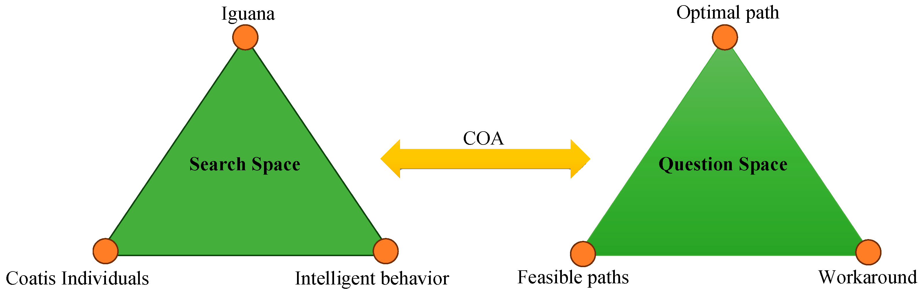
3.1. Coati Optimization Algorithm (COA)

The coati optimization algorithm (COA) [23] is a novel optimization algorithm proposed by Dehghani et al. It is inspired by the predatory and evasion behaviors of coatis in nature. The algorithm is divided into two phases: the first phase simulates the coatis’ behavior of catching iguanas, representing the exploration behavior; the second phase simulates the coatis’ behavior of evading predators, representing the exploitation behavior.

(1)

Hunting and attacking strategy on iguana

When coatis hunt iguanas, they act in groups. A portion of the group climbs trees to catch iguanas, which causes the frightened iguanas to fall from the trees. The remaining coatis that are on the ground then continue to capture the fallen iguanas. This hunting strategy divides the coati population into two parts, each searching for prey. In the design of the COA, it is assumed that half of the coatis climb trees to catch iguanas, while the other half remains on the ground to catch the falling iguanas. The iguanas on the trees are set as the known best solutions of the population, and when the iguanas fall to the ground, they are abstracted as randomly falling into a certain position in the search space.

The behavior of the coatis catching iguanas in the trees can be simulated by the following formula:

$$X_i^{P1}:x_{i,j}^{P1}=x_{i,j}+r·(Xbes{t}_j-I·x_{i,j})$$

(14)

where $x_{i,j}^{P1}$ represents the j-th dimension of the i-th coati in the first stage; $Xbes{t}_j$ represents the j-th dimension of the population’s current best solution; and I is a random value that can take values {1, 2}. This model indicates that during an iteration, the coati’s new hunting position searches towards the best value, potentially moving away from or closer to it.

After the iguanas fall to the ground, the coatis on the ground continue to hunt the iguanas. At this time, the position of the iguana is a random position in the search space, represented by the following formula:

$$X^G:x_j^G=l{b}_j+r·(u{b}_j-l{b}_j)$$

(15)

where $X^G$ represents the randomly generated position of the iguana; $l{b}_j$ represents the lower bound of the j-th dimension’s range; $u{b}_j$ represents the upper bound of the j-th dimension’s range; and r denotes the random value in [0, 1].

Based on the random position of the fallen iguana, the coatis will search for prey nearby. This process can be expressed as follows:

$$X_i^{P1}:x_{i,j}^{P1}=\left\{\begin{array}{l}{x}_{i,j}+r·\left(X_j^G-I·x_{i,j}\right),F_{X^G}<F_i\hfill \\ x_{i,j}+r·\left(x_{i,j}-X_j^G\right),else\hfill \end{array}\right.$$

(16)

where I is a random value that can take values {1, 2}; r denotes the random value in [0, 1]; $F_{X^G}$ is the cost function value of the newly generated iguana position; $F_i$ is the cost function value of the original population; r is a random value within the range (0, 1); and $x_{i,j}$ represents the j-th dimension of the i-th individual’s data.

When the newly detected position is better than the original position, the new position will be updated in the population, which is shown in Equation (7).

$$X_i=\left\{\begin{array}{ll}{X}_i^{P1},\hfill & F_i^{P1}<F_i\hfill \\ X_i,\hfill & else.\hfill \end{array}\right.$$

(17)

where $X_i$ denotes the position of the i-th coatis; $X_i^{P1}$ represents the position that the coatis detected in phase 1; and $F$ denotes the cost value corresponding to the position of the coatis.

(2)

The process of escaping from predators

When coatis are hunted by predators, they randomly jump to nearby positions to evade them. This process can be simulated by the following formula:

$$l{b}_j^{local}={\displaystyle \frac{l{b}_j}{t}},u{b}_j^{local}={\displaystyle \frac{u{b}_j}{t}}$$

(18)

$$X_i^{P2}:x_{i,j}^{P2}=x_{i,j}+(1-2r)·\left(l{b}_j^{local}+r·\left(u{b}_j^{local}-l{b}_j^{local}\right)\right)$$

(19)

where $l{b}_j^{local}$ and $u{b}_j^{local}$ define the escape range of the coatis and $X_i^{P2}$ represents the position after the coatis have been attacked. This behavior exhibits good exploitation, enabling the algorithm to fully explore the already searched space to find the best solution.

$$X_i=\left\{\begin{array}{ll}{X}_i^{P2},\hfill & F_i^{P2}<F_i\hfill \\ X_i,\hfill & else.\hfill \end{array}\right.$$

(20)

where $X_i$ denotes the position of the i-th coatis; $X_i^{P2}$ represents the position that the coatis detected in phase 2; and $F$ denotes the cost value corresponding to the position of the coatis.

3.2. Improvement Strategies

The COA, in its predation phase, defaults to splitting the population into two parts: one of them updates individuals guided by the best value, and the other part updates the algorithm using random values. The results detected by these two parts are different, but the algorithm does not fully utilize this diverse information. Therefore, this paper proposes a dynamic opposite learning search method for population interaction. Additionally, the COA’s method of searching for the best solution is relatively simple, which may not be sufficient to obtain high-quality paths in path planning problems. This paper introduces a covariance matrix search, which analyzes the probabilistic distribution of the best solutions over generations and explores areas more likely to contain the best solution through differential evolution. The two improvement strategies are introduced below.

3.2.1. Dynamic Opposite Learning Search (DOL)

Dynamic opposite learning (DOL) is an improved strategy based on opposition-based learning (OBL) [29]. It aims to accelerate the population’s convergence process and improve the global search capability by introducing opposite points. The basic idea of opposition-based learning is to consider both the current solution and its opposite solution simultaneously, thereby increasing the coverage of the search space and improving the probability of finding the optimal solution. Dynamic opposite learning further integrates the dynamic information of the population, flexibly adjusting the generation of opposite points according to the current state of the population, making it more adaptable to the optimization process. The formula is as follows:

$$x^{dol}=x+r^1(r^2{x}^o-x)$$

(21)

$$x^o=a+b-x$$

(22)

where $x^o$ is the opposite operator, $a$ and $b$ represent the lower and upper bounds of the decision variables, respectively.

In the COA, the population is divided into two parts during the predation phase, and there is a lack of interaction between the populations during the predation process simulation. This causes the algorithm to not fully utilize known solutions. After the population completes its respective predation, the other part of the population performs differential dynamic opposite learning, and its update formula is as follows:

$$X_i^{new}=X_i+r_c(r_c(lowerbound+upperbound-X_i^{op})-X_i^{op})$$

(23)

During the search process, the individuals of the two populations are ranked according to their fitness values, so the i-th individual in population $X_i^1$ corresponds to the i-th individual in the pre-half population. When updating the i-th individual in $X_i^2$, the corresponding $X_i^{op}$ is the i-th individual in the later-half population, and similarly, when updating the i-th individual in $X^2$, the corresponding $X_i^{op}$ is the i-th individual in the pre-half population. $r_c$ is a random number that obeys the Cauchy distribution.

3.2.2. Covariance Matrix Learning Search (CML)

The covariance matrix learning strategy is an improvement method proposed in recent years [30]. It dynamically adjusts the search direction and step size by analyzing the distribution of the optima for generations, enhancing the algorithm’s global search capability and robustness. The basic idea of this strategy is to use the covariance matrix to describe the distribution characteristics of the population and, through this information, guide mutations and selections toward the area where the optimal solution is most likely to exist. Figure 4 shows the principle of CML.

The covariance matrix refers to an archive matrix, which is composed of the concatenation of the elite group within l iterations, and its formula is as follows:

$$A^t=B^t\cup B^{t-1}\cup \cdots \cup B^{t-l+1}$$

(24)

The purpose of obtaining the covariance matrix is to analyze the potential probability distribution of the optimal solution in the solution space. Thus, covariance analysis can be performed on the obtained archive matrix.

$${\mu }^{t+1}={\displaystyle \frac{1}{\left|A^t\right|}}·{\displaystyle \sum _{i=1}^{\left|A^t\right|}{A}_i^t}$$

(25)

$$M^{t+1}={\displaystyle \frac{1}{\left|A^t\right|}}·{\displaystyle \sum _{i=1}^{\left|A^t\right|}(A_i^t-{\mu }^{t+1}){(A_i^t-{\mu }^{t+1})}^T}$$

(26)

$$M=C·\Lambda ·C^T$$

(27)

$$Xtem{p}_i^t=X_i^t·C$$

(28)

where $M$ is the covariance matrix and $\mu$ is the mean vector of the archive matrix. After obtaining the covariance matrix, it is decomposed into characteristic matrices $C$. $Xtem{p}_i^t$ represents the transformed individual position of the i-th individual in the t-th iteration.

By performing differential evolution searches in the transformed space, the best solution can be found more efficiently. During differential mutation, the information from the covariance matrix is used to adjust the direction and magnitude of the mutation vector, better adapting to the structure of the search space. Based on the eigenvalues and eigenvectors of the covariance matrix, the selection strategy is dynamically adjusted, enabling the population to explore the solution space more uniformly and avoid falling into local optima. The following equation gives the specific update formula.

$$Xtem{p}_{i,j}^{t+1}=\left\{\begin{array}{l}Xtem{p}_{r_1,j}^t+r_c(Xtem{p}_{r_2,j}^t-Xtem{p}_{r_3,j}^t), if rand<r_n\hfill \\ Xtem{p}_{i,j}^t+r_c(Xtem{p}_{r_1,j}^t-Xtem{p}_{i,j}^t)+r_c(Xtem{p}_{r_2,j}^t-Xtem{p}_{r_3,j}^t), otherwise\hfill \end{array}\right.$$

(29)

where t denotes the iteration; $r_c$ is a random number that obeys the Cauchy distribution; $r_n$ is a random number that obeys the normal distribution; and $r_1, r_2, r_3$ denote random integers in the range [1, N], where N represents the number of population. The introduction of this strategy can effectively improve the search efficiency and solution quality of the differential evolution algorithm, particularly in complex high-dimensional optimization problems, showing stronger adaptability and robustness.

Once the search is complete, the results also need to be converted to the original coordinate system using Equation (30).

$$X_i^{t+1}=Xtem{p}_i^{t+1}·C^T$$

(30)

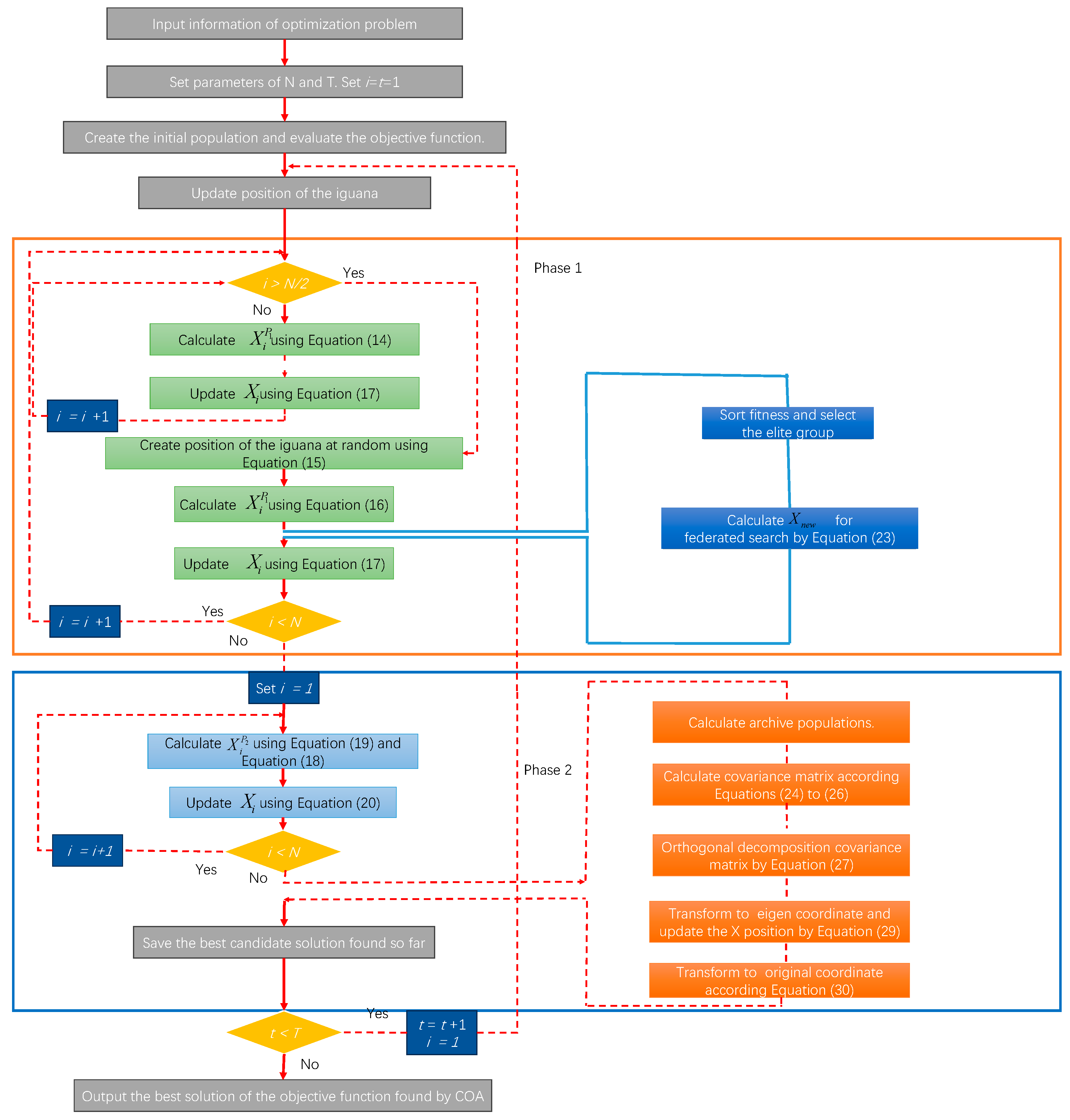
3.3. Overall Framework for Path Planning Based on the OCLCOA

The algorithm proposed in this paper addresses the issues of insufficient interaction between populations and weak exploitation ability in the original COA by introducing two modification strategies. The first is the dynamic opposite search, which further searches the locations detected by the population during the predation phase of the original COA. The second is the covariance matrix learning, which constructs a covariance matrix using information from the known best solution, extracts features, and uses this information to search for the area with the highest probability of containing the better solution. Through the reasonable introduction of the above strategies, the opposite covariance learning coatis optimization algorithm (OCLCOA) proposed in this paper is obtained. The algorithm’s approach to solving the UAV path planning problem is as follows: Using the spatial transformation method in Section 2, the OLBCOA needs to determine the positions of z′ and y′ in space to determine the position of the path points in space. After cubic spline interpolation, enough path points are obtained. An individual of the population represents a feasible path in the algorithm. The algorithm finds the best solution in the search space through its detection, i.e., the shortest path. The overall framework of the algorithm is as follows:

Step 1: Initialize the algorithm parameters, determine the starting and target positions of the UAV, load the environment information, and initialize the population.

Step 2: Execute the predation strategy of the original COA. The first N/2 individuals explore the search space guided by the known best solution, while the latter N/2 explore the search space guided by random positions in the search space. Compare the generated positions with the original positions to determine which solution is of better quality and guide the algorithm to explore the search space based on the best of the three solutions as the updated result.

Step 3: Execute the dynamic opposite learning search proposed in this paper. Sort the two parts of the population based on the cost function, and the individuals in the same rank act as each other’s opposite operator source during exploration.

Step 4: Execute the evasion strategy of the original COA. Individuals randomly explore nearby positions and compare the new positions with the original positions to determine which is better and select the best as the search result for this phase.

Step 5: Execute the covariance update strategy. Focus on searching the area with the highest probability of containing the best solution by analyzing the probability distribution of the best solution, improving the quality of the algorithm’s solution.

Step 6: Check if the maximum number of iterations has been reached. If not, continue from Step 2; otherwise, return the known best solution.

The algorithm flowchart is shown in Figure 5.

3.4. Time Complexity Analysis

Algorithm complexity is an effective analysis method to measure the efficiency of algorithms, which describes the growth trend of the time and space required for algorithm execution with the increase in input data size.

In this paper, the problem scale of the algorithm is mainly determined by the number of populations and the number of individual decisional variables. Now N represents the population and m represents the number of individual decision variables, and the total number of iterations is denoted as T, then the frequency in the initialization process of the algorithm is $O\left(Nm\right)$, the frequency of the predation stage is $O\left(NmT\right)$, the access frequency of calculating the position of falling iguana is $O\left(NmT/2\right)$, and the access frequency of the algorithm is $O\left(NmT\right)$, the degree of dynamic opposition search is $O\left(NmT\right)$, and the access frequency of the covariance matrix is $O\left(NmT\right)$. In this paper, the total time access frequency of the proposed algorithm is $O\left(Nm+7/2NmT\right)$, that is, the time complexity of the algorithm is $O\left(NmT\right)$, which indicates the proposed algorithm is a linear time algorithm, so it can be regarded as an efficient algorithm.

4. Experiment and Results

4.1. Experimental Setup

The experimental parameters were standardized, with a population size of 150, 100 iterations, and 10 key points for algorithmic optimization. The cost function parameters were set as follows: $w_1=2$, $w_2=20$, $w_3=2$, $w_4=300$. The path was determined using cubic spline interpolation, resulting in 50 path points. To evaluate the effectiveness of the proposed algorithm, five different algorithms were selected for comparison. In the experiment, each algorithm was run independently 10 times, with the results of all runs recorded. The figure for the path of this experiment focused on the result with the smallest fitness value out of the 10 independent runs. All experiments were conducted on a personal computer equipped with an AMD Ryzen 7 6800H processor with Radeon graphics, a 3.20 GHz processor, and 16 GB of RAM, source from Lenovo and the experiments were constructed in MATLAB R2021b (9.11.0.1769968).

The five algorithms tested included the original COA, the newly proposed Artificial Hummingbird Algorithm (AHA) [22], the Sinh Cosh Optimizer (SCHO) inspired by the Sinh and Cosh functions [42], the classical Grey Wolf Optimizer (GWO) [21], and the Improved Salp Swarm Algorithm (ISSA) [43]. The parameters for these algorithms are detailed in the

Table 1. The parameters of algorithms used for the experiment.

Algorithm	Parameters
SCHO	$u_t=0.388$, $m=0.45$, $n=0.5$, $p=10$, $q=9$, $\alpha =4.6$, $\beta =1.55$
GWO	/
AHA	/
ISSA	$p_{foll}=0.2$, $p_{pion}=0.3$
COA	/
OCLCOA	${\mu }_{cr}=0.5$${\mu }_f=0.5$

, all of which were derived from their respective original papers.

The setting of the risk level and the information in

Table 2. The information on the threat areas.

Case Number	Threat Center	Threat Radius	Threat Level
Case 1	(42, 44), (54, 58), (63, 39), (83, 80)	7, 10, 8, 8	12, 8, 10, 10
Case 2	(20, 40), (65, 44), (40, 45), (60, 75)	12, 9, 11, 8	12, 8, 10, 10
Case 3	(50, 20), (65, 24), (40, 45), (60, 75)	12, 9, 11, 8, 9, 8	12, 8, 10, 10, 11, 9
	(40, 70), (39, 18)
Case 4	(50,20), (65,55), (40,45), (60,75), (40,70), (39,18)	12, 9, 15, 15, 9, 8	12, 8, 100,000, 100,000, 11, 9

refer to the paper published by Niu et al. [37]. For simplicity of calculation, a larger number is set instead of infinity for the high-risk restricted flight zones where entry is absolutely prohibited.

4.2. Experimental Result

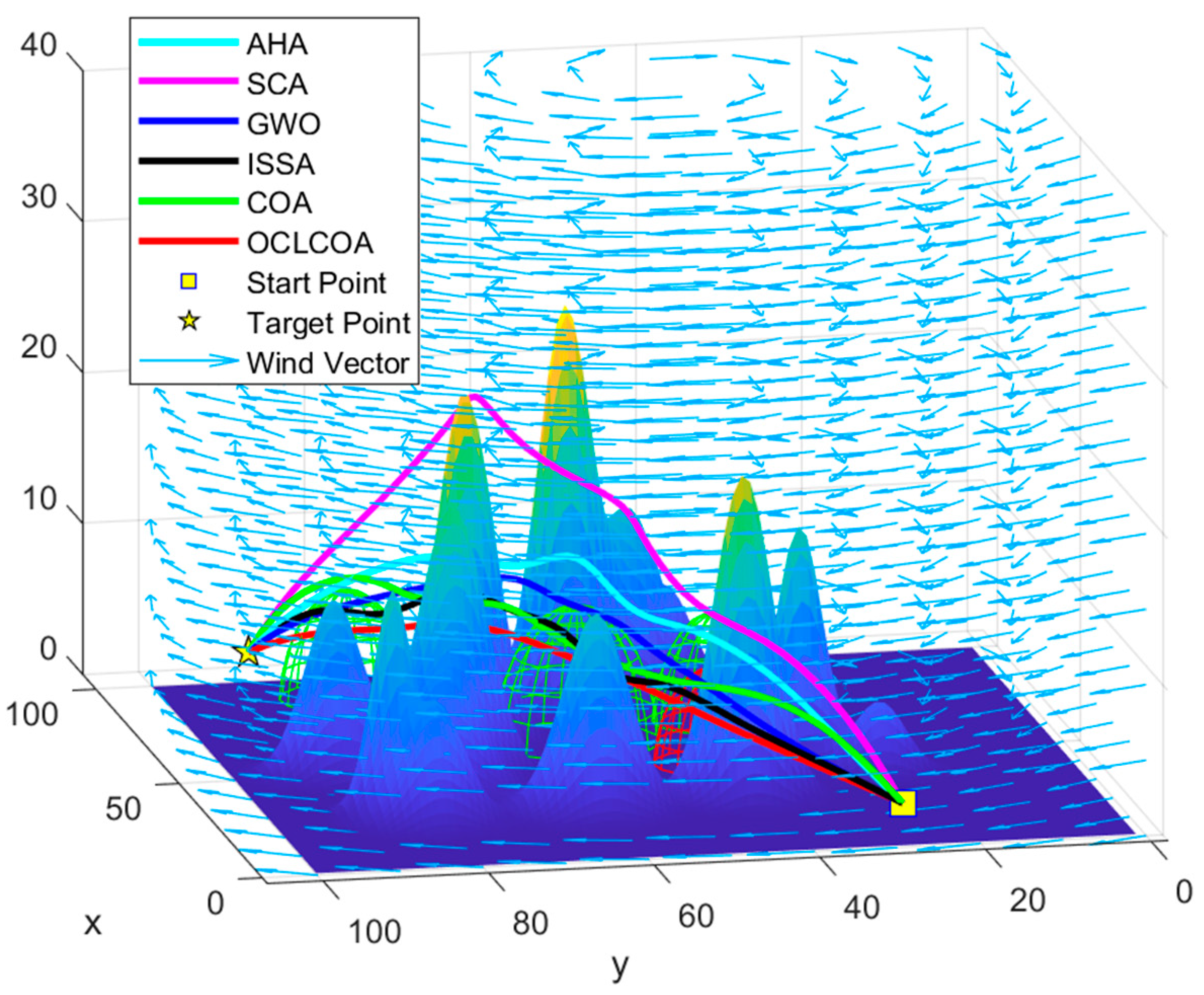
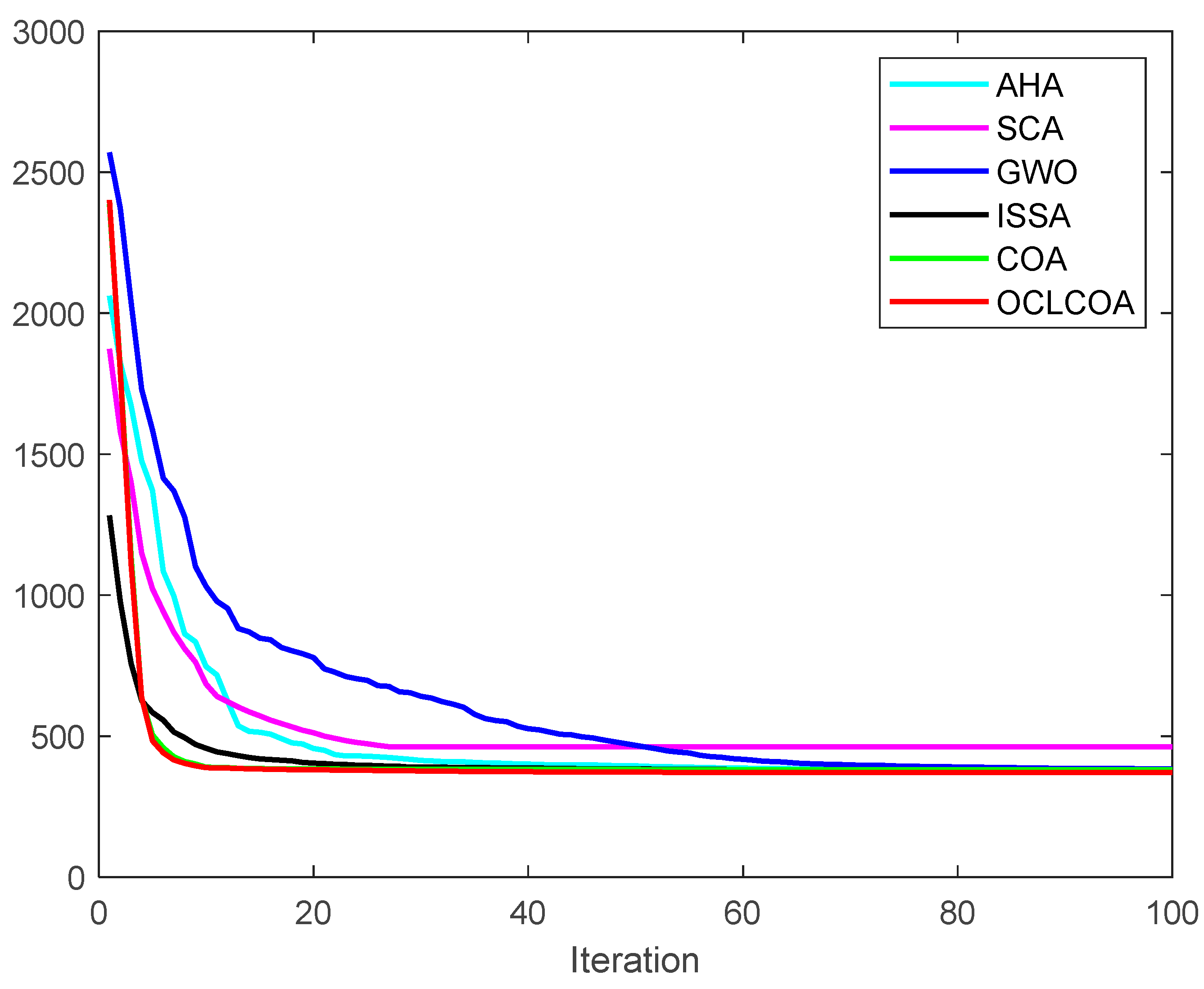
(1)

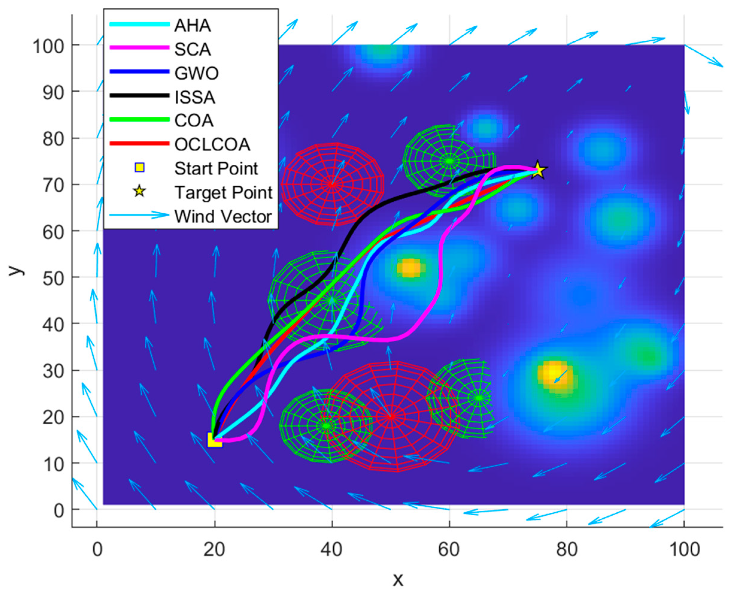
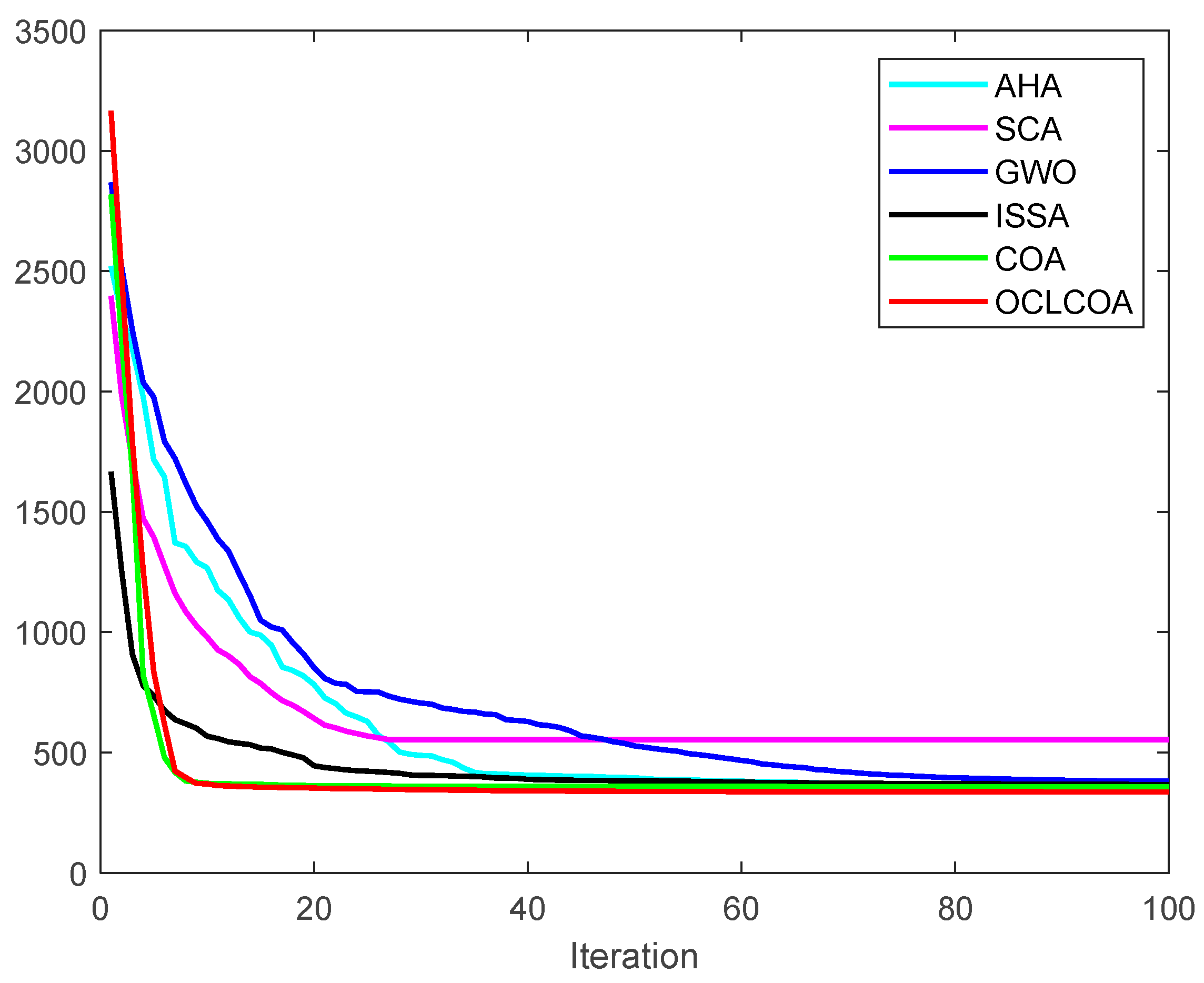
Analysis of the experimental results of Case 1

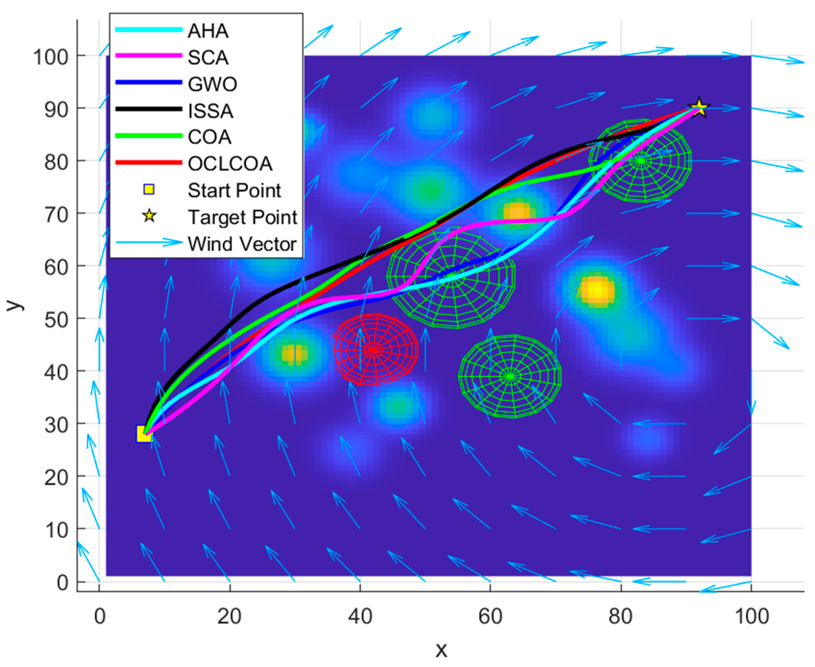
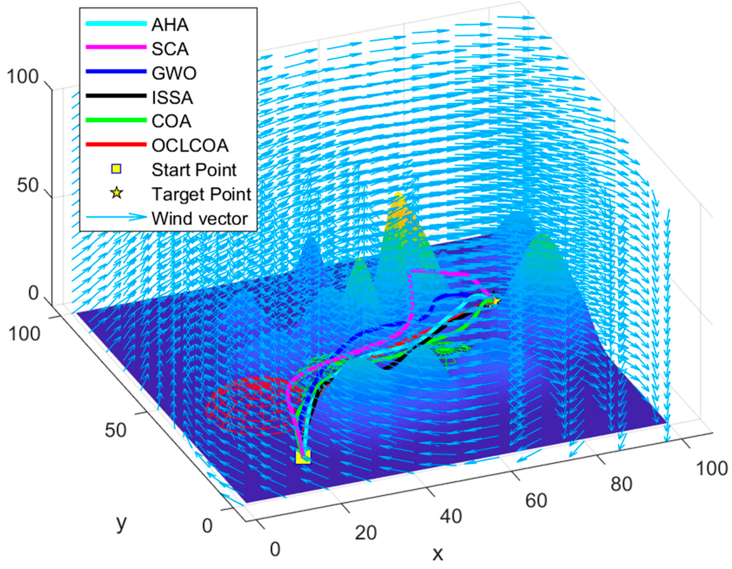
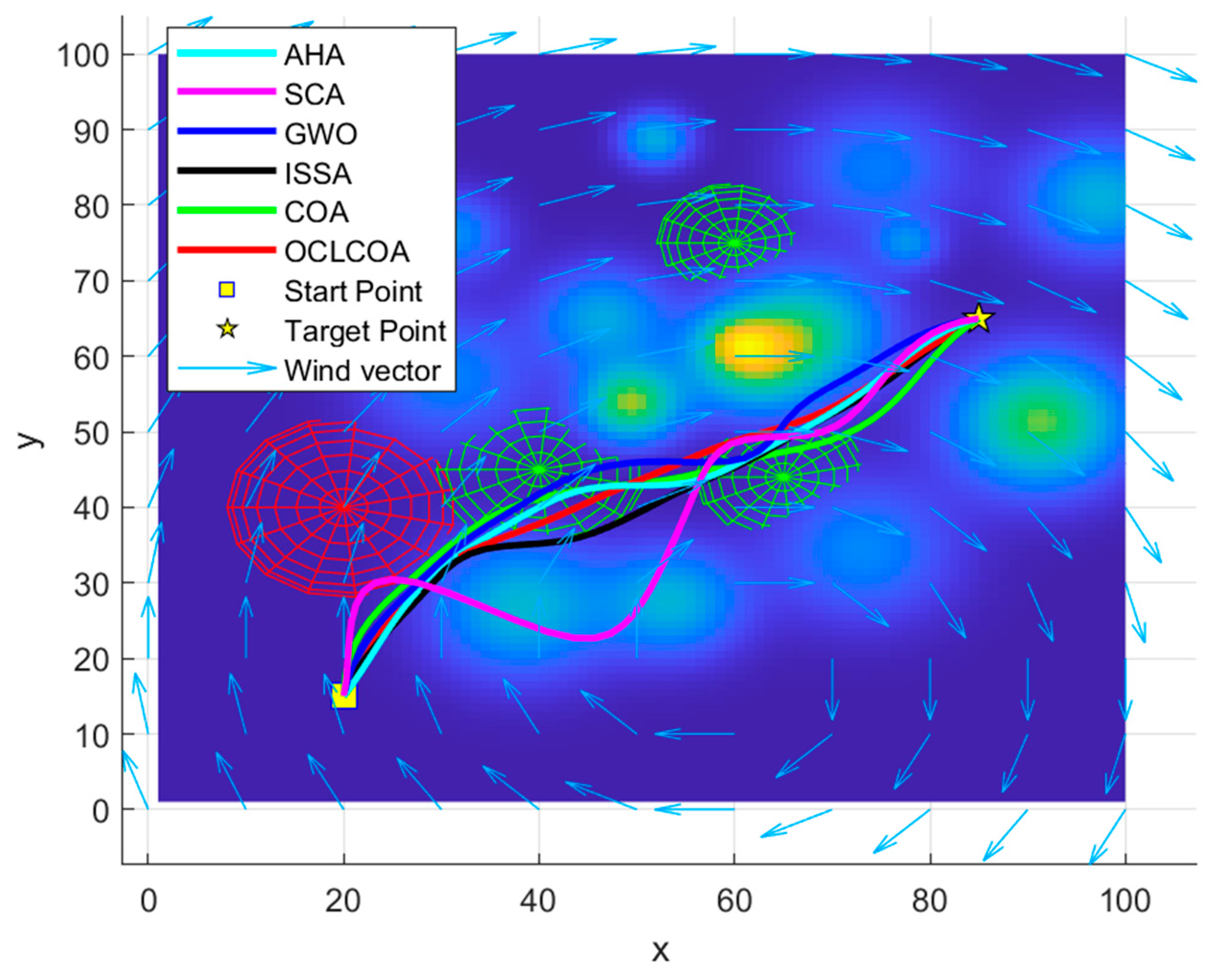
In Case 1, the island terrain was generated randomly by Equation (2), the environment with the flight-restricted area parameters detailed in Table 2, and wind field information provided in

Table 3. The information on the wind.

Case Number	Center of Wind	Vortex Force
Case 1	(90, 40, z)	100
Case 2	(60, 20, z)	100
Case 3	(60, 20, z), (95, 95, z)	100
Case 4	(60, 20, z), (95, 95, z)	100

. From Figure 6 and Figure 7, it can be seen that all UAV paths avoid the flight-restricted area and do not collide with the island terrain. The distinction between different algorithms is reflected in the paths and whether they align with the wind direction. The OCLCOA produces the shortest path among all the tested algorithms, which helps reduce the time to reach the search and rescue area, maximizing the use of the golden rescue time and increasing the survival rate of distressed individuals. The UAV path generated by the OCLCOA is smooth and aligns with the wind direction, which helps save energy to increase the rescue coverage area. The OCLCOA has the lowest flight altitude, which assists the UAVs in capturing small targets and reduces interference from water surface reflections or complex lighting conditions on the sensing equipment’s performance, thereby allowing the UAVs to more accurately identify distressed individuals.

From

Table 4. The cost function value from 10 independent run times for all algorithms in Case 1.

	AHA	GWO	ISSA	SCHO	COA	OCLCOA
best	373.606	370.8464	368.3236	388.6394	369.5416	363.8627
worst	386.7746	394.7373	393.3506	698.881	389.9641	374.2758
mean	377.2344	384.3177	378.5627	462.1609	380.8371	370.3685
std	3.8415	7.042375	8.182222	88.50879	6.909722	3.7746

, it can be observed that the average value of the OCLCOA is lower than that of the other compared algorithms, indicating that the performance of the OCLCOA is superior. Additionally, the best and worst values of the OCLCOA are also better than those of the other compared algorithms, indicating that the overall performance of the OCLCOA surpasses that of the others. Although the improvement is in the range of 1% to 3%, the path quality is better than the original algorithm. The convergence speed reflects the effectiveness of the algorithm’s search strategy, indicating that the algorithm can quickly find the best solution. As seen in Figure 8, the convergence speed of both the OCLCOA and COA is faster than the other algorithms, with the OCLCOA showing a quicker convergence than the COA, representing an improvement in search capability.

(2)

Analysis of the experimental results of Case 2

In Case 2, the island terrain is continuous. The data from

Table 5. The cost function value from 10 independent run times for all algorithms in Case 2.

	AHA	GWO	ISSA	SCHO	COA	OCLCOA
best	358.7826	318.3921	302.7449	406.6434	359.5944	297.2654
worst	384.2930	485.0109	396.2466	813.3052	553.3509	300.6004
mean	368.0918	376.4741	345.7796	560.0747	449.6301	298.1347
std	9.4373	48.22716	35.50665	138.136	62.93447	1.0972

show that the path cost planned by the OCLCOA in Case 2 is lower than that of the other compared algorithms, indicating that its performance is superior and has good stability. The OCLCOA consistently stabilized around 297 with a variance of less than 1.0972. Compared with the original COA, the best value improved by 17.33%, the average value improved by 33.69%, and the variance is much lower than that of other algorithms, which proves that the algorithm proposed in this paper has an improvement effect.

Figure 9 and Figure 10 illustrate the paths generated by each algorithm in this scenario, with the OCLCOA producing the shortest path. The algorithm proposed in this paper performs well in terms of path smoothness and wind direction adaptation, which are advantageous for improving the survival rate of distressed individuals. In this scenario, it can be seen from Figure 11 that the convergence speed of all algorithms is reduced, but the OCLCOA remains relatively fast, showing that its search strategy is effective.

(3)

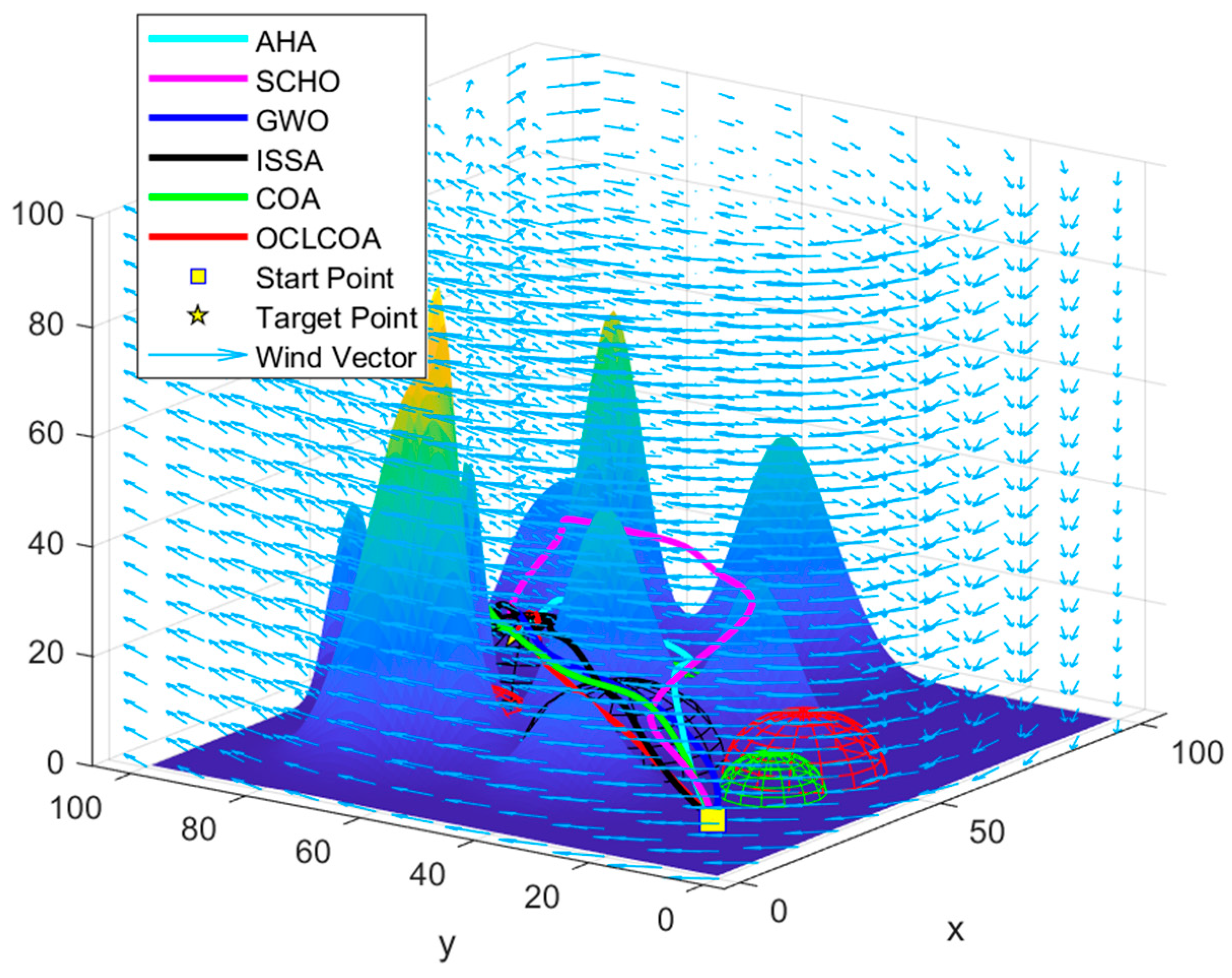
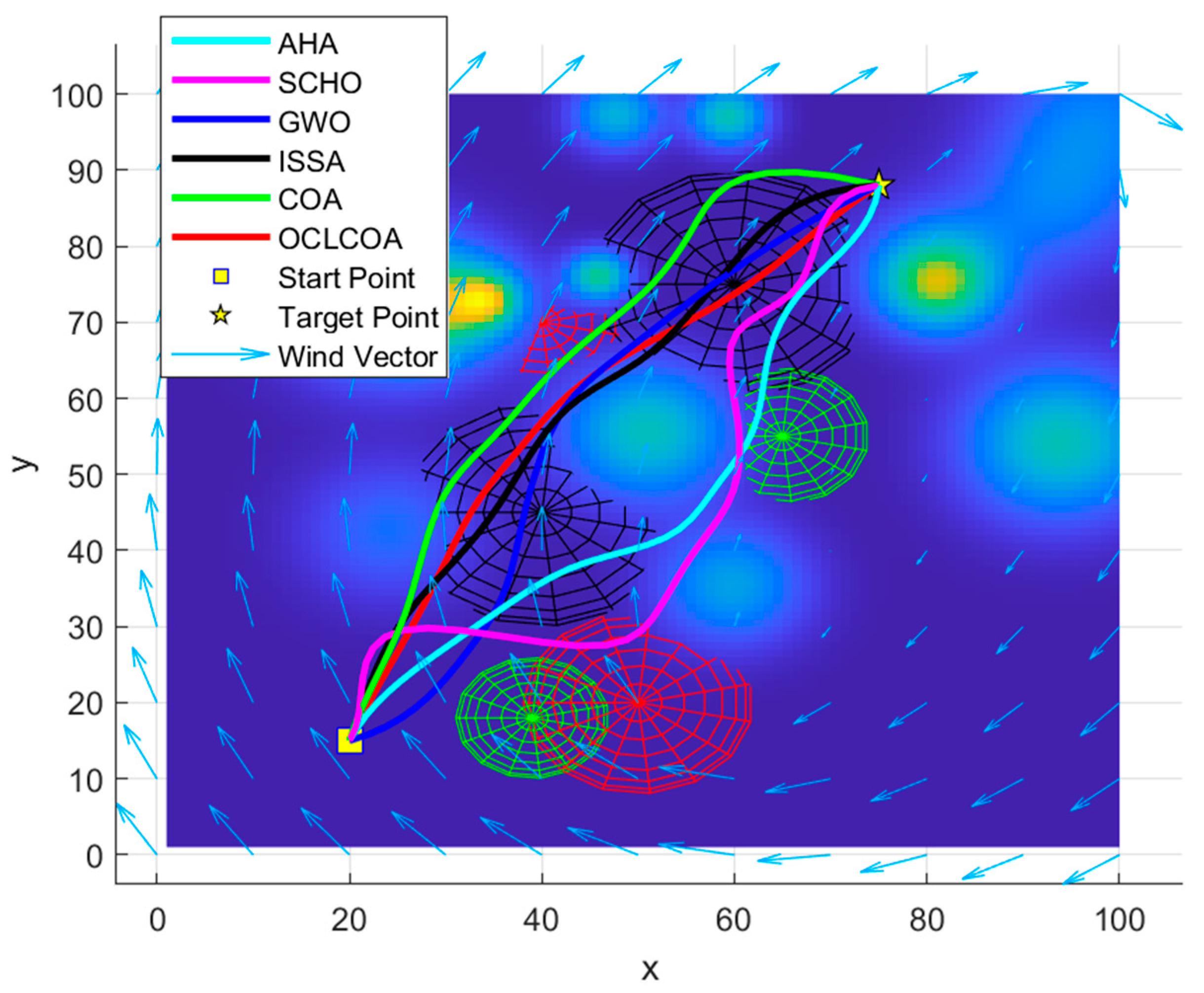
Analysis of the experimental results of Case 3

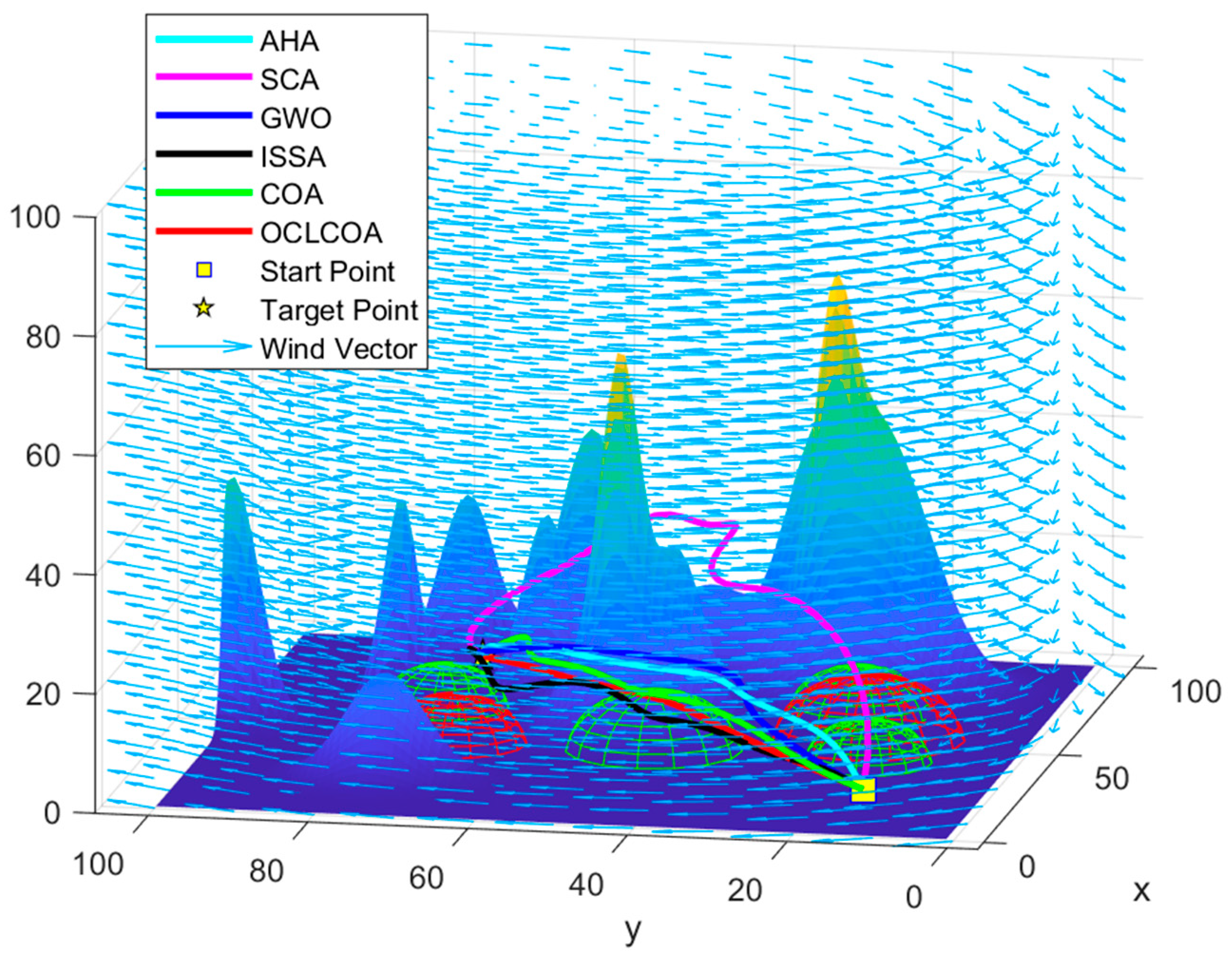
In Case 3, as shown in

Table 6. The cost function value from 10 independent run times for all algorithms in Case 3.

	AHA	GWO	ISSA	SCHO	COA	OCLCOA
best	347.8254	350.4642	345.5671	414.7658	343.48	336.3658
worst	363.8949	404.9287	394.4875	794.1183	372.6724	338.0068
mean	355.7923	381.1501	366.7454	553.8437	357.4407	336.7215
std	5.6371	19.22943	19.47307	139.6807	11.22852	0.5207

, the OCLCOA outperforms other algorithms in terms of the average, best, and worst values across 10 independent runs. This indicates that the performance of the proposed algorithm is generally superior to the comparison algorithms. The proposed algorithm had the lowest cost and demonstrated strong stability, consistently stabilizing around 336 with a variance of 0.5207, indicating strong stability of the algorithm in this scenario. Compared with the original COA, the average value improved by 5.80%, and the variance is much lower than other algorithms. These results confirm that the proposed improvements enhance the quality of UAV path planning.

The island terrain in the environmental model was also randomly generated. The wind field was designed with two centers, leading to different effects compared to the previous test cases. From Figure 12 and Figure 13, it can be seen that the paths generated by the OCLCOA exhibit good smoothness, with the shortest path length, the lowest altitude, and alignment with the wind direction. This demonstrates that the paths generated by the OCLCOA handle various influencing factors well, making it suitable for UAV maritime rescue path planning. Figure 14 shows the variation of the cost function value with the number of iterations for each algorithm in this scenario, and it can be seen that the convergence of OCLCOA is fast.

(4)

Analysis of the experimental results of Case 4

In Case 4, the black spherical area represents the absolute no-entry area, the red area is the medium-risk flight-restricted area, and the green area is the low-risk flight-restricted area. It can be seen from Figure 15 and Figure 16 that none of the UAV paths fly into the flight-restricted area, but there are still distinctions between the paths generated by different algorithms. The OCLCOA consistently produces the shortest path among all the algorithms, with no unnecessary turns, and its direction aligns with the wind. The flight altitude is lower than that of the comparison algorithms, which can reduce rescue time and conserve energy for subsequent search tasks, thereby increasing the probability of rescuing distressed individuals. Although the convergence speed, which is shown in Figure 17, in this case is not high, the algorithm successfully avoids local optima and identifies the best path.

From the cost function value shown in

Table 7. The cost function value from 10 independent run times for all algorithms in Case 4.

	AHA	GWO	ISSA	SCHO	COA	OCLCOA
best	365.5839	357.6008	359.8623	415.449	371.3288	349.2881
worst	380.6820	595.3989	406.8791	908.5643	451.8913	360.0667
mean	373.0015	415.0495	377.5996	592.7857	398.7402	354.1212
std	4.3792	75.55398	13.98372	195.4778	25.28233	3.941439

, when considering the average value, the best value, or the worst value, the result is better than other comparative algorithms, and compared with the original COA, the best value is improved by 5.94%, the average value is improved by 11.19%, and the variance is even much lower than the other algorithms. This all demonstrates that the proposed algorithm performs well in solving path planning problems.

4.3. Discussion

This study explores the application of swarm intelligence algorithms to UAV path planning in a 3D offshore search and rescue environment. UAVs have significant applications in ocean monitoring, particularly when equipped with remote sensing technology. Their powerful monitoring capabilities enable the rapid and accurate identification of specific targets in the marine environment, making them highly valuable for rescue missions in offshore scenarios. An important challenge is determining how the UAV can reach the target location efficiently.

This study developed a coastal marine environment model that includes island terrain, wind simulations, and flight-restricted areas to realistically replicate actual conditions. A series of evaluation metrics for UAV paths was also established to guide the algorithm in searching for the best path. Building on the COA, this study introduced new strategies to address its potential shortcomings, thereby improving its effectiveness in solving UAV path planning problems in offshore environments. Unlike robot path planning in two-dimensional planes, UAVs require a 3D environmental model to fully leverage their advantages. Although there has been prior research on UAV path planning in 3D environments, it has not accounted for the influence of wind, which is a critical factor in offshore UAV path planning.

This study offers a solution for UAV path planning in offshore environments, considering both the advantages of UAVs and the impact of wind. Overall, compared to the original algorithm, the average value of the OCLCOA improved by 13.36%, and the best value improved by 6.72%, with the average path length reduced by 18.00%, which is shown in

Table 8. Comparison of the path mean length.

	AHA	SCHO	GWO	ISSA	COA	OCLCOA
Case 1	112.0129	148.8177	115.7833	113.2852	113.4264	108.7025
Case 2	96.0262	195.8193	122.0939	110.2201	139.5378	88.5176
Case 3	92.6224	177.8489	107.0696	98.4565	95.965	84.6041
Case 4	108.3449	195.6559	127.2776	111.132	123.9482	99.8476

. The best value and average value of the OCLCOA in Case 1 increased by 1.54% and 2.75%, respectively. However, in Case 2, the performance of the OCLCOA showed a significant improvement, with the best value and average value increasing by 17.33% and 33.69%, respectively. The algorithm’s effectiveness has only been validated through mathematical simulation, and further testing is necessary to ensure the proposed solution’s reliability.

Additionally, applying these research findings to practical scenarios presents challenges, such as how to handle dynamic obstacles, integrate the research into UAV control systems, manage UAV hardware to ensure the UAV follows the planned path, and efficiently search the target area. The implementation of UAV rescue systems will require time and continued efforts from researchers.

5. Conclusions

To establish an efficient UAV coastal search and rescue system, solving the UAV path planning problem is a fundamental step. This study proposed a method for UAV path planning by developing a coastal environment model to simulate real marine conditions. Building on the COA, improvements were made to address its shortcomings in path planning. The introduction of a dynamic opposition-based search and covariance search mechanisms enhanced the COA’s search efficiency, as evidenced by its superior performance compared to other algorithms tested in this study.

The proposed method addresses the global UAV path planning problem; however, complex marine environments present unknown dynamic obstacles that could affect UAV flight. Future research should focus on dynamic UAV path planning—determining the key points of the UAV path within a global static environment model and then dynamically planning paths between these key points to further enhance UAV flight path reliability. There are existing algorithms, such as the D* algorithm, that address real-time path planning, but their performance has room for improvement. Future advancements may involve integrating these algorithms with deep learning to achieve faster and more accurate dynamic path planning. In subsequent research, we will also include real-world validation to further demonstrate the utility of the algorithm.

References

1. Wen, H.; Shi, Y.; Wang, S.; Chen, T.; Di, P.; Yang, L. Route Planning for UAVs Maritime Search and Rescue Considering the Targets Moving Situation. Ocean Eng. 2024, 310, 118623. [Google Scholar] [CrossRef]
2. Shao, M.; Wu, B.; Li, Y.; Jiang, X. Research on the Deployment of Professional Rescue Ships for Maritime Traffic Safety under Limited Conditions. J. Mar. Sci. Eng. 2024, 12, 497. [Google Scholar] [CrossRef]
3. Yang, Z.; Yu, X.; Dedman, S.; Rosso, M.; Zhu, J.; Yang, J.; Xia, Y.; Tian, Y.; Zhang, G.; Wang, J. UAV Remote Sensing Applications in Marine Monitoring: Knowledge Visualization and Review. Sci. Total Environ. 2022, 838, 155939. [Google Scholar] [CrossRef] [PubMed]
4. Yan, Y.; Chen, X.; Shi, M.; Li, R. A Decision Support System Architecture for Intelligent Driven Unmanned Aerial Vehicles Maritime Search and Rescue. In Proceedings of the 2024 10th International Symposium on System Security, Safety, and Reliability (ISSSR), Xiamen, China, 30–31 March 2024; pp. 424–428. [Google Scholar]
5. Yan, M.; Yuan, H.; Xu, J.; Yu, Y.; Jin, L. Task Allocation and Route Planning of Multiple UAVs in a Marine Environment Based on an Improved Particle Swarm Optimization Algorithm. EURASIP J. Adv. Signal Process. 2021, 2021, 94. [Google Scholar] [CrossRef]
6. Messmer, M.; Zell, A. Evaluating UAV Path Planning Algorithms for Realistic Maritime Search and Rescue Missions. In Proceedings of the 2024 International Conference on Unmanned Aircraft Systems (ICUAS), Chania, Greece, 4–7 June 2024. [Google Scholar]
7. Aggarwal, S.; Kumar, N. Path Planning Techniques for Unmanned Aerial Vehicles: A Review, Solutions, and Challenges. Comput. Commun. 2020, 149, 270–299. [Google Scholar] [CrossRef]
8. Yang, L.; Qi, J.; Xiao, J.; Yong, X. A Literature Review of UAV 3D Path Planning. In Proceedings of the 11th World Congress on Intelligent Control and Automation, Shenyang, China, 29 June–4 July 2014; pp. 2376–2381. [Google Scholar]
9. Sun, C.-C.; Jan, G.E.; Leu, S.-W.; Yang, K.-C.; Chen, Y.-C. Near-Shortest Path Planning on a Quadratic Surface With O(Nłog n) Time. IEEE Sens. J. 2015, 15, 6079–6080. [Google Scholar] [CrossRef]
10. Zafar, M.N.; Mohanta, J.C. Methodology for Path Planning and Optimization of Mobile Robots: A Review. Procedia Comput. Sci. 2018, 133, 141–152. [Google Scholar] [CrossRef]
11. Noto, M.; Sato, H. A Method for the Shortest Path Search by Extended Dijkstra Algorithm. In Proceedings of the Smc 2000 Conference Proceedings. 2000 IEEE International Conference On Systems, Man and Cybernetics. “Cybernetics Evolving to Systems, Humans, Organizations, and Their Complex Interactions” (cat. no.0), Nashville, TN, USA, 8–11 October 2000; Volume 3, pp. 2316–2320. [Google Scholar]
12. Warren, C.W. Fast Path Planning Using Modified A* Method. In Proceedings of the 1993 IEEE International Conference on Robotics and Automation, Atlanta, GA, USA, 2–6 May 1993; Volume 2, pp. 662–667. [Google Scholar]
13. Pan, Z.; Zhang, C.; Xia, Y.; Xiong, H.; Shao, X. An Improved Artificial Potential Field Method for Path Planning and Formation Control of the Multi-UAV Systems. IEEE Trans. Circuits Syst. II Express Briefs 2022, 69, 1129–1133. [Google Scholar] [CrossRef]
14. Gasparetto, A.; Boscariol, P.; Lanzutti, A.; Vidoni, R. Path Planning and Trajectory Planning Algorithms: A General Overview. In Motion and Operation Planning of Robotic Systems: Background and Practical Approaches; Carbone, G., Gomez-Bravo, F., Eds.; Springer International Publishing: Cham, Switzerland, 2015; pp. 3–27. ISBN 978-3-319-14705-5. [Google Scholar]
15. Schmid, L.; Pantic, M.; Khanna, R.; Ott, L.; Siegwart, R.; Nieto, J. An Efficient Sampling-Based Method for Online Informative Path Planning in Unknown Environments. IEEE Robot. Autom. Lett. 2020, 5, 1500–1507. [Google Scholar] [CrossRef]
16. Tsardoulias, E.G.; Iliakopoulou, A.; Kargakos, A.; Petrou, L. A Review of Global Path Planning Methods for Occupancy Grid Maps Regardless of Obstacle Density. J. Intell. Robot. Syst. 2016, 84, 829–858. [Google Scholar] [CrossRef]
17. Kesavan, V.; Kamalakannan, R.; Sudhakarapandian, R.; Sivakumar, P. Heuristic and Meta-Heuristic Algorithms for Solving Medium and Large Scale Sized Cellular Manufacturing System NP-Hard Problems: A Comprehensive Review. Mater. Today Proc. 2020, 21, 66–72. [Google Scholar] [CrossRef]
18. Puente-Castro, A.; Rivero, D.; Pazos, A.; Fernandez-Blanco, E. A Review of Artificial Intelligence Applied to Path Planning in UAV Swarms. Neural Comput. Appl. 2022, 34, 153–170. [Google Scholar] [CrossRef]
19. Tang, J.; Liu, G.; Pan, Q. A Review on Representative Swarm Intelligence Algorithms for Solving Optimization Problems: Applications and Trends. IEEECAA J. Autom. Sin. 2021, 8, 1627–1643. [Google Scholar] [CrossRef]
20. Adam, S.P.; Alexandropoulos, S.-A.N.; Pardalos, P.M.; Vrahatis, M.N. No Free Lunch Theorem: A Review. In Approximation and Optimization: Algorithms, Complexity and Applications; Demetriou, I.C., Pardalos, P.M., Eds.; Springer International Publishing: Cham, Switzerland, 2019; pp. 57–82. ISBN 978-3-030-12767-1. [Google Scholar]
21. Mirjalili, S.; Mirjalili, S.M.; Lewis, A. Grey Wolf Optimizer. Adv. Eng. Softw. 2014, 69, 46–61. [Google Scholar] [CrossRef]
22. Zhao, W.; Wang, L.; Mirjalili, S. Artificial Hummingbird Algorithm: A New Bio-Inspired Optimizer with Its Engineering Applications. Comput. Methods Appl. Mech. Eng. 2022, 388, 114194. [Google Scholar] [CrossRef]
23. Dehghani, M.; Montazeri, Z.; Trojovská, E.; Trojovský, P. Coati Optimization Algorithm: A New Bio-Inspired Metaheuristic Algorithm for Solving Optimization Problems. Knowl.-Based Syst. 2023, 259, 110011. [Google Scholar] [CrossRef]
24. Emary, E.; Zawbaa, H.M.; Hassanien, A.E. Binary Grey Wolf Optimization Approaches for Feature Selection. Neurocomputing 2016, 172, 371–381. [Google Scholar] [CrossRef]
25. Masehian, E.; Sedighizadeh, D. A Multi-Objective PSO-Based Algorithm for Robot Path Planning. In Proceedings of the 2010 IEEE International Conference on Industrial Technology, Vina del Mar, Chile, 14–17 March 2010; pp. 465–470. [Google Scholar]
26. Qtaish, A.; Braik, M.; Albashish, D.; Alshammari, M.T.; Alreshidi, A.; Alreshidi, E.J. Enhanced Coati Optimization Algorithm Using Elite Opposition-Based Learning and Adaptive Search Mechanism for Feature Selection. Int. J. Mach. Learn. Cybern. 2024. [Google Scholar] [CrossRef]
27. Abou Houran, M.; Salman Bukhari, S.M.; Zafar, M.H.; Mansoor, M.; Chen, W. COA-CNN-LSTM: Coati Optimization Algorithm-Based Hybrid Deep Learning Model for PV/Wind Power Forecasting in Smart Grid Applications. Appl. Energy 2023, 349, 121638. [Google Scholar] [CrossRef]
28. Emam, M.M.; Houssein, E.H.; Samee, N.A.; Alohali, M.A.; Hosney, M.E. Breast Cancer Diagnosis Using Optimized Deep Convolutional Neural Network Based on Transfer Learning Technique and Improved Coati Optimization Algorithm. Expert Syst. Appl. 2024, 255, 124581. [Google Scholar] [CrossRef]
29. Xu, Y.; Yang, X.; Yang, Z.; Li, X.; Wang, P.; Ding, R.; Liu, W. An Enhanced Differential Evolution Algorithm with a New Oppositional-Mutual Learning Strategy. Neurocomputing 2021, 435, 162–175. [Google Scholar] [CrossRef]
30. Deng, L.; Liu, S. Incorporating Q-Learning and Gradient Search Scheme into JAYA Algorithm for Global Optimization. Artif. Intell. Rev. 2023, 56, 3705–3748. [Google Scholar] [CrossRef]
31. Yang, T.; Jiang, Z.; Sun, R.; Cheng, N.; Feng, H. Maritime Search and Rescue Based on Group Mobile Computing for Unmanned Aerial Vehicles and Unmanned Surface Vehicles. IEEE Trans. Ind. Inform. 2020, 16, 7700–7708. [Google Scholar] [CrossRef]
32. Cho, S.W.; Park, H.J.; Lee, H.; Shim, D.H.; Kim, S.-Y. Coverage Path Planning for Multiple Unmanned Aerial Vehicles in Maritime Search and Rescue Operations. Comput. Ind. Eng. 2021, 161, 107612. [Google Scholar] [CrossRef]
33. Zhang, X.; Duan, H. An Improved Constrained Differential Evolution Algorithm for Unmanned Aerial Vehicle Global Route Planning. Appl. Soft Comput. 2015, 26, 270–284. [Google Scholar] [CrossRef]
34. Li, W.; Tan, M.; Wang, L.; Wang, Q. A Cubic Spline Method Combing Improved Particle Swarm Optimization for Robot Path Planning in Dynamic Uncertain Environment. Int. J. Adv. Robot. Syst. 2020, 17, 1–12. [Google Scholar] [CrossRef]
35. Lian, J.; Yu, W.; Xiao, K.; Liu, W. Cubic Spline Interpolation-Based Robot Path Planning Using a Chaotic Adaptive Particle Swarm Optimization Algorithm. Math. Probl. Eng. 2020, 2020, 1849240. [Google Scholar] [CrossRef]
36. Li, X.; Yu, S. Three-Dimensional Path Planning for AUVs in Ocean Currents Environment Based on an Improved Compression Factor Particle Swarm Optimization Algorithm. Ocean Eng. 2023, 280, 114610. [Google Scholar] [CrossRef]
37. Niu, Y.; Yan, X.; Wang, Y.; Niu, Y. Three-Dimensional UCAV Path Planning Using a Novel Modified Artificial Ecosystem Optimizer. Expert Syst. Appl. 2023, 217, 119499. [Google Scholar] [CrossRef]
38. Stodola, P.; Nohel, J. Reconnaissance in Complex Environment with No-Fly Zones Using a Swarm of Unmanned Aerial Vehicles. In Modelling and Simulation for Autonomous Systems, Proceedings of the 8th International Conference, MESAS 2021, Virtual Event, 13–14 October 2021, Revised Selected Papers; Mazal, J., Fagiolini, A., Vasik, P., Turi, M., Bruzzone, A., Pickl, S., Neumann, V., Stodola, P., Eds.; Springer International Publishing: Cham, Switzerland, 2022; pp. 308–321. [Google Scholar]
39. Niu, Y.; Yan, X.; Wang, Y.; Niu, Y. Three-Dimensional Collaborative Path Planning for Multiple UCAVs Based on Improved Artificial Ecosystem Optimizer and Reinforcement Learning. Knowl.-Based Syst. 2023, 276, 110782. [Google Scholar] [CrossRef]
40. Chung, H.-M.; Maharjan, S.; Zhang, Y.; Eliassen, F.; Strunz, K. Placement and Routing Optimization for Automated Inspection with Unmanned Aerial Vehicles: A Study in Offshore Wind Farm. IEEE Trans. Ind. Inform. 2021, 17, 3032–3043. [Google Scholar] [CrossRef]
41. Zhang, H.; Shi, X. An Improved Quantum-Behaved Particle Swarm Optimization Algorithm Combined with Reinforcement Learning for AUV Path Planning. J. Robot. 2023, 2023, e8821906. [Google Scholar] [CrossRef]
42. Bai, J.; Li, Y.; Zheng, M.; Khatir, S.; Benaissa, B.; Abualigah, L.; Wahab, M.A. A Sinh Cosh Optimizer. Knowl.-Based Syst. 2023, 282, 111081. [Google Scholar] [CrossRef]
43. Tudose, A.M.; Sidea, D.O.; Picioroaga, I.I.; Anton, N.; Bulac, C. Increasing Distributed Generation Hosting Capacity Based on a Sequential Optimization Approach Using an Improved Salp Swarm Algorithm. Mathematics 2024, 12, 48. [Google Scholar] [CrossRef]
Figure 1. Schematic diagram of the key point generation principle.
Jmse 12 01676 g001
Figure 2. Risk level calculation schematic.
Jmse 12 01676 g002
Figure 3. Correspondence map between the search space and question space.
Jmse 12 01676 g003
Figure 4. The search direction found by covariance matrix learning.
Jmse 12 01676 g004
Figure 5. The flow chart of the proposed OCLOA for path planning.
Jmse 12 01676 g005
Figure 6. The path result of Case 1.
Jmse 12 01676 g006
Figure 7. The top view of the path result of Case 1.
Jmse 12 01676 g007
Figure 8. The iteration result of Case 1.
Jmse 12 01676 g008
Figure 9. The path result of Case 2.
Jmse 12 01676 g009
Figure 10. The top view of the path result of Case 2.
Jmse 12 01676 g010
Figure 11. The iteration result of Case 2.
Jmse 12 01676 g011
Figure 12. The path result of Case 3.
Jmse 12 01676 g012
Figure 13. The top view of the path result of Case 3.
Jmse 12 01676 g013
Figure 14. The iteration result of Case 3.
Jmse 12 01676 g014
Figure 15. The path result of Case 4.
Jmse 12 01676 g015
Figure 16. The top view of the path result of Case 4.
Jmse 12 01676 g016
Figure 17. The iteration result of Case 4.
Jmse 12 01676 g017