Intelligent Fault Diagnosis Method for Constant Pressure Variable Pump Based on Mel-MobileViT Lightweight Network

Abstract

The sound signals of hydraulic pumps contain abundant key information reflecting their internal mechanical states. In environments characterized by high temperatures or high-speed rotation, or where sensor deployment is challenging, acoustic sensors offer non-contact and flexible arrangement features. Therefore, this study aims to develop an intelligent fault diagnosis method for hydraulic pumps based on acoustic signals. Initially, the Adaptive Chirp Mode Decomposition (ACMD) method is employed to remove environmental noise from the acoustic signals, enhancing the feature signals. Subsequently, the Mel spectrum is extracted as the acoustic fingerprint features of various fault states of the hydraulic pump, and these features are used to train the MobileViT network, achieving accurate identification of the different fault modes. The results indicate that the proposed Mel-MobileViT model effectively identifies and classifies various faults in constant pressure variable pumps, outperforming other models. This study not only provides an efficient and reliable intelligent method for the fault diagnosis of critical industrial equipment such as hydraulic pumps, but also offers new perspectives on the application of deep learning in acoustic pattern analysis.

1. Introduction

Hydraulic servo systems, with their high power density, rapid response, and high rigidity, have been widely applied in fields such as heavy machinery, manufacturing, and shipbuilding [1]. With the modernization of hydraulic technology, while the production efficiency has significantly improved, the interconnectivity between components within the same equipment and across different devices has also increased. A fault in any component within the system could lead to production halts or even cause accidents. As an indispensable part of the hydraulic system, the health of the hydraulic pump directly affects the overall system performance, making the fault diagnosis of hydraulic pumps crucial [2,3,4,5].

The primary fault types in hydraulic pumps include loosened slippers, plungers, slipper pads, and rolling bearings. These faults can be detected through vibration, pressure, and sound signals [6,7]. Among these, sound signal acquisition is a low-cost, non-intrusive method that covers a wide range and does not require interrupting or altering the operational state of the equipment. Consequently, in recent years, sound-based fault diagnosis of mechanical equipment has garnered significant attention [8,9,10]. For instance, Tang et al. [11] used envelope analysis and order tracking to detect bearing faults, validating that both vibration and acoustic signals are suitable for diagnosing low-speed bearing faults, and found that acoustic signals have a higher signal-to-noise ratio under various operating conditions. Hou et al. [12] proposed a method for acoustic fingerprint feature recognition based on acoustic signals. This method uses clustering significance indicators to guide the intelligent selection of dynamic thresholds, automatically identifying periodic signals generated by bearing faults and tracking changes in speed and time in real-time. Elasha et al. [13] employed adaptive filtering and spectral kurtosis techniques on the acoustic signals from helicopter gearbox bearings, successfully extracting fault characteristic information and demonstrating the advantages of acoustic signals compared to vibration signals.

With the rapid development of artificial intelligence technology, significant achievements have been made in intelligent fault diagnosis methods based on acoustic signals [14,15]. Smith et al. [16] proposed an intelligent bearing fault diagnosis method based on acoustic features. This method involves extracting the Mel spectrogram from denoised acoustic signals and using a convolutional neural network (CNN) as the classifier to accurately identify motor bearing faults. Taylor et al. [17] utilized a CNN to extract features from the acoustic signals of drilling machines and optimized the feature set through neighborhood component analysis, further enhancing the performance of machine learning classifiers and providing an effective method for the early detection of drill bit faults. Islam et al. [18] decomposed acoustic signals using the discrete wavelet packet transform, converted the defect-to-health ratio of sub-bands into image data, and inputted it into a CNN for bearing fault diagnosis. Similarly, Kumar et al. [19] extracted grayscale images of acoustic signals and utilized a CNN to diagnose centrifugal pump faults, demonstrating the practicality and efficiency of this method. In addition to supervised learning methods, semi-supervised and unsupervised learning techniques are crucial tools in the field of fault diagnosis, especially effective when the fault data is scarce or difficult to label effectively. Unsupervised methods, including clustering algorithms, autoencoders, and Principal Component Analysis (PCA), do not require labeled data for fault detection and diagnosis. These methods are particularly suitable for anomaly detection and fault prediction in complex systems. Ji and colleagues [20] have developed a fault diagnosis method based on parallel sparse filtering. This approach enhances the extraction of sparse features from acoustic signals by adding another normalization direction to the sparse filtering process. Experiments have confirmed that this method is effective for diagnosing faults in rotating machinery. Shao and others [21] have developed a semi-supervised model for assessing the severity of faults in hydraulic pumps. This model uses labeled data from the source domain to pre-train a convolutional neural network, and employs adversarial training with unlabeled data in the target domain to achieve adaptive updating and the recognition of cross-domain fault severity.

During the collection of sound signals, they are more susceptible to interference from external environmental noise. Consequently, numerous studies have utilized signal decomposition methods to reduce noise interference and enhance data accuracy. These algorithms can adaptively extract modal components, selecting effective modes and eliminating noise. Empirical Mode Decomposition (EMD) has been widely used in signal processing-based fault diagnosis methods. However, EMD may experience modal mixing when processing signals containing random noise and lacks rigorous mathematical descriptions and theoretical support [22,23]. Therefore, Drag and others proposed the Variational Mode Decomposition (VMD) method [24]. VMD effectively reduces modal mixing by decomposing signals into modes with specific bandwidths, resulting in decomposed modes that possess greater physical significance. However, the VMD algorithm requires a predetermined number of modes, which may pose challenges in practical applications. To overcome this limitation, Chen and others developed the Adaptive Chirp Mode Decomposition (ACMD) method [25,26]. This method can adaptively adjust the chirp rate, more accurately matching and decomposing specific frequency components in signals, effectively separating fault characteristic signals from noise, thus becoming an effective noise reduction tool in fault diagnosis.

Based on the analysis, it is evident that fault diagnosis techniques based on acoustic signals have achieved initial results and show a broad development prospect. This paper focuses on constant pressure variable pumps and proposes a lightweight intelligent fault diagnosis method for hydraulic pumps based on acoustic fingerprint features and the MobileViT model. By integrating signal processing methods with artificial intelligence technologies, this approach significantly enhances the accuracy and efficiency of fault diagnosis in constant pressure variable pumps, providing a safeguard for the stable operation of hydraulic systems.

The structure of this paper is as follows. Section 2 discusses the fault mechanisms of constant pressure variable pumps as well as the basic theories of the MobileViT and ACMD algorithms. Section 3 introduces the main processes of the Mel-MobileViT method. Section 4 details the setup of fault simulation experiments for constant pressure variable pumps, the collection of acoustic data, and the construction of Mel samples. Section 5 presents the diagnostic results of the Mel-MobileViT model and a comparative analysis with different networks. Finally, Section 6 concludes the paper and discusses its limitations.

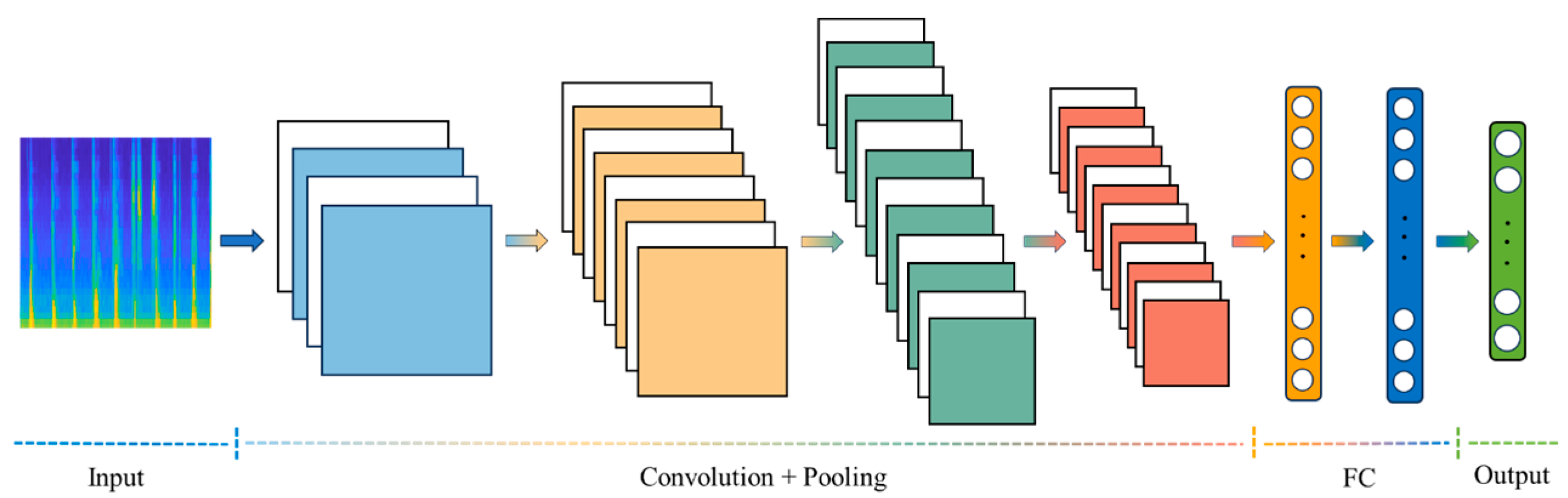
2. Based on the Basic Theory of the Mel-MoblieViT Fault Diagnosis Method

This chapter primarily discusses the theoretical basis of the intelligent fault diagnosis method proposed. Initially, the paper provides a detailed introduction to the common types of faults and their mechanisms in constant pressure variable pumps. Additionally, it introduces the Adaptive Chirp Mode Decomposition algorithm, used for noise reduction, and the MobileViT lightweight convolutional neural network, which classifies fault patterns based on acoustic fingerprint features for fault diagnosis.

2.1. Failure Mechanism of Constant Pressure Variable Pumps

The hydraulic pump, as the core power component of a hydraulic system, converts mechanical energy into hydraulic pressure, continuously supplying energy to actuators within the system. It plays an indispensable role in industrial production and transportation. When a hydraulic pump fails, it can disrupt operations, leading to the prolonged downtime of mechanical equipment, which reduces production efficiency and introduces safety risks. In severe cases, such failures can even result in injury or loss of life. The main failure modes of constant pressure variable pumps include loose slipper failure, plunger wear, slipper wear, and rolling bearing failure.

1.

Loose slipper failure: This occurs when there is excessive clearance between the pump’s slipper socket and the plunger ball head, leading to periodic vibration and impact between the plunger ball head and the slipper socket during operation.

2.

Slipper wear failure: Normally, an oil film of a certain thickness exists between the swashplate and the slipper in a hydraulic pump, preventing direct metal contact and reducing friction. When the oil film pressure drops due to various factors, the oil film fails, leading to accelerated wear between the slipper and the swashplate.

3.

Plunger wear failure: Wear between the plunger and the cylinder block increases the gap, leading to higher leakage. When the plunger cavity connects with the high-pressure discharge port during the pump rotation, the increased leakage causes hydraulic shock, altering the vibration behavior of the pump casing.

4.

Rolling bearing failure: The degradation or failure of rolling bearings can be caused by several factors, such as lubrication failure or overloading. Common failure modes include fatigue spalling, plastic deformation, wear, fractures, and overheating.

2.2. Introduction to MobileViT Model

As illustrated in Figure 1, a typical CNN architecture includes an input layer, convolutional layers, pooling layers, fully connected layers, and an output layer [27,28,29,30]. However, as models continually iterate and increase in complexity, the number of parameters and computational costs also rises, posing significant challenges for deployment in resource-constrained environments such as embedded devices. To address this issue, researchers have explored various strategies to reduce the scale and complexity of CNNs, including techniques such as structural pruning, parameter quantization, and knowledge distillation [31,32,33,34].

Although these technologies have achieved significant success in reducing computational burdens and model size, there are still some limitations in maintaining model accuracy. Researchers have found that the Vision Transformer (ViT), which uses a self-attention mechanism, exhibits immense potential in the visual domain, but architectures based on self-attention typically have large parameter counts and computational demands. In this context, the introduction of the MobileViT model addresses this gap, effectively combining the inductive bias advantages of CNNs with the global receptive capabilities of the ViT, while also featuring a lightweight network architecture, making it highly suitable for intelligent fault diagnosis systems on resource-constrained edge computing devices. According to experimental data, MobileViT outperforms traditional CNNs and ViT architectures in multiple tasks and datasets [35].

The MobileViT network architecture, as shown in Figure 2, primarily consists of standard convolutions, MV2 (i.e., the inverted residual structure from MobileNetV2), MobileViT blocks, a global pooling layer, and a fully connected layer. The MobileViT block, as the core component of the model, aims to extract both local and global features with a reduced parameter count. This process mimics the standard convolution operation’s unfold, local processing, and fold steps. However, unlike traditional methods, the MobileViT block replaces the conventional local processing step with L-stacked Transformers that perform global processing, mainly to capture the global dependencies. This combination of local and global processing effectively encodes the local and global information. Traditional methods typically project patches and use Transformers to learn global information between the patches, a process that can lose the image’s inductive bias and requires more parameters, resulting in a model that is both deep and wide. The MobileViT block combines the local feature extraction capabilities of convolution with the global modeling capacity of the ViT. Furthermore, MobileViT ingeniously integrates the inverted residual module of MobileNetV2 and effectively designs the sequence of the MV2 block and MobileViT block positions to represent the interaction of local and global visual information. The MobileViT convolution calculation is as follows:

1.

The first component is the local representation module. For an input $X\in R^{H\ast W\ast C}$, it undergoes consecutive operations of Conv-3 × 3 and Conv-1 × 1, resulting in an output $X_L\in R^{H\ast W\ast d}$, where the 3 × 3 convolution is used for local feature modeling, and the 1 × 1 convolution is used to adjust the number of channels.

2.

The next component is the global representation module, which uses the unfold operation to expand $X_L$ into N non-overlapping patches $X_U\in R^{P\ast N\ast d}$. Here, $P=wh$ (where ℎ and w represent the height and width of each patch, respectively), and $N=WH/P$. Subsequently, L-stacked Transformers are used to focus on the global information of $X_U$, resulting in an output $X_G\in R^{P\ast N\ast d}$. Finally, the fold operation is applied to produce $X_F\in R^{H\ast W\ast d}$, which has the same dimensions as $X_L$.

3.

The final component is the fusion module, which first uses a 1 × 1 convolution to adjust the number of channels back to the original size. Then, it concatenates this with the original input feature map along the channel dimension through a shortcut branch. Lastly, a 3 × 3 convolution fuses the local and global features to produce the output $Y\in R^{H\ast W\ast C}$.

Figure 2. MobileViT network architecture.

Figure 2. MobileViT network architecture.

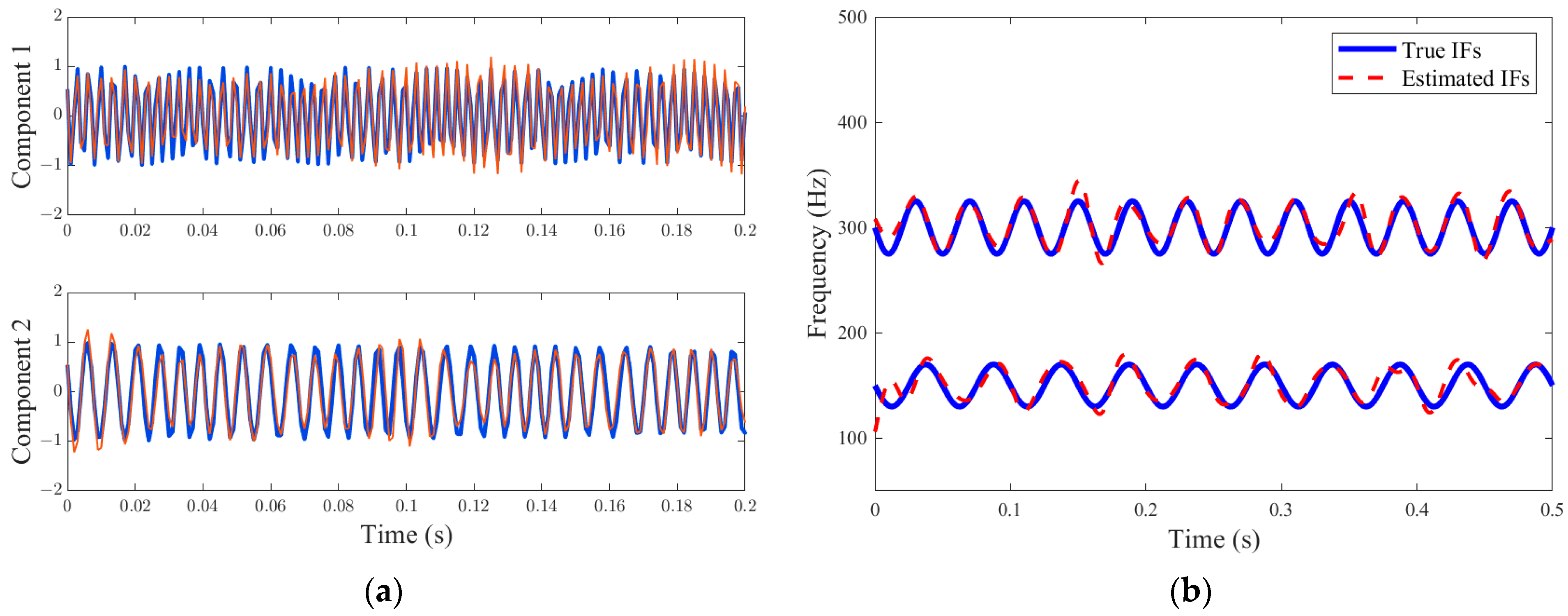
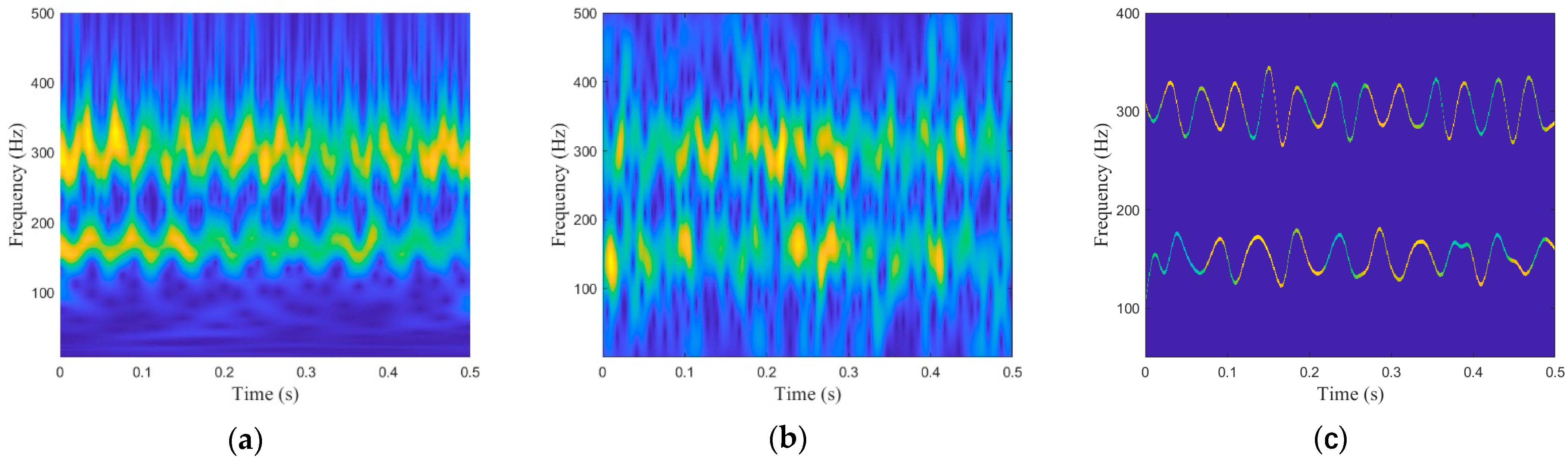
2.3. Adaptive Chirped Mode Decomposition Principle

Non-stationary signals typically consist of multiple sub-signals, which are referred to as chirp modes in ACMD. Each chirp mode can be modeled as an Amplitude Modulated-Frequency Modulated (AM-FM) signal.

$$x(t)={\displaystyle \sum _{m=1}^M{x}_m}(t)={\displaystyle \sum _{m=1}^M{a}_m}(t)\cos \left[2\pi {\displaystyle {\int }_0^t{f}_m}(s)\mathrm{d}s+{\phi }_m\right]$$

(1)

where $x\left(t\right)$ represents the superposition of M chirp modes; $a_m\left(t\right)$, $f_m\left(t\right),$ and ${\phi }_m$ are the instantaneous amplitude, instantaneous frequency, and initial phase of the m-th component, respectively.

Based on the trigonometric identity, Equation (1) can be rewritten as:

$$x(t)={\displaystyle \sum _{m=1}^M{\mu }_m}(t)\cos \left[2\pi {\displaystyle {\int }_0^t{\tilde{f}}_m}(s)\mathrm{d}s\right]+{\zeta }_m(t)\sin \left[2\pi {\displaystyle {\int }_0^t{\tilde{f}}_m}(s)\mathrm{d}s\right]$$

(2)

$$\left\{\begin{array}{l}{\mu }_m(t)=a_m(t)\cos \left\{2\pi {\displaystyle {\int }_0^t\left[f_m(s)-{\tilde{f}}_m(s)\right]}\mathrm{d}s+{\phi }_m\right\}\\ {\zeta }_m(t)=-a_m(t)\sin \left\{2\pi {\displaystyle {\int }_0^t\left[f_m(s)-{\tilde{f}}_m(s)\right]}\mathrm{d}s+{\phi }_m\right\}\end{array}\right.$$

(3)

where ${\mu }_m(t)$ and ${\zeta }_m(t)$ are the two demodulation signals; $\cos \left[2\pi {\displaystyle {\int }_0^t{\tilde{f}}_m}(s)\mathrm{d}s\right]$ and $\sin \left[2\pi {\displaystyle {\int }_0^t{\tilde{f}}_m}(s)\mathrm{d}s\right]$ are the two demodulation operators; and ${\tilde{f}}_m\left(s\right)$ is the frequency function of the operator.

When $f_m\left(s\right)={\tilde{f}}_m\left(s\right)$, ${\mu }_m(t)$ and ${\zeta }_m(t)$ become two slowly varying baseband signals, each with the narrowest bandwidth. Therefore, the fundamental concept of ACMD is to extract the target signal components and estimate their instantaneous frequency (IF) by minimizing the bandwidth.

$$\begin{array}{l}\underset{{\alpha }_m,{\beta }_m{\tilde{f}}_m}{\min }\left\{{‖{\mu }_m^{″}(t)‖}_2^2+{‖{\zeta }_m^{″}(t)‖}_2^2+\tau {‖x(t)-x_m(t)‖}_2^2\right\}\\ \mathrm{s}.\mathrm{t}.x_m(t)={\mu }_m(t)\cos \left[2\pi {\displaystyle {\int }_0^t{\tilde{f}}_m}(s)\mathrm{d}s\right]+{\zeta }_m(t)\sin \left[2\pi {\displaystyle {\int }_0^t{\tilde{f}}_m}(s)\mathrm{d}s\right]\end{array}$$

(4)

where ${‖·‖}_2^2$ denotes the L2 norm, ${‖x\left(t\right)-x_m\left(t\right)‖}_2^2$ represents the residual energy after removing the estimated component, and $\tau$ is a weighting factor, with $\tau >0$.

Assuming the signal consists of N sample points, the discretization of the above equation can be expressed as

$$\underset{y_m,f_m}{\min }\left\{{‖\Theta y_m‖}_2^2+\tau {‖x-G_m{y}_m‖}_2^2\right\}$$

(5)

where $\Theta =\left[\begin{array}{cc}D& 0\\ 0& D\end{array}\right]$, $\mathbf{D}$ is a second-order difference matrix;

$$y_m={\left[{\mu }_m^{\mathrm{T}}{\zeta }_m^{\mathrm{T}}\right]}^{\mathrm{T}},\mathrm{where}\left\{\begin{array}{l}{\mu }_m={\left[{\mu }_m\left(t_0\right),{\mu }_m\left(t_1\right),\cdots ,{\mu }_m\left(t_{N-1}\right)\right]}^{\mathrm{T}}\\ {\zeta }_m=\left[{\zeta }_m\left(t_0\right),{\zeta }_m\left(t_1\right),\cdots \right.{\left.,{\zeta }_m\left(t_{N-1}\right)\right]}^{\mathrm{T}}\end{array}\right.;$$

$$x={\left[x\left(t_0\right),x\left(t_1\right),\cdots ,x\left(t_{N-1}\right)\right]}^{\mathrm{T}};$$

and

$$G_m=\left[C_m,S_m\right],$$

where

$$\left\{\begin{array}{l}{\mathit{C}}_m=\mathrm{diag}\left[\cos \left({\theta }_m\left(t_0\right)\right)\cdots \cos \left({\theta }_m\left(t_{N-1}\right)\right)\right]\\ {\mathbf{S}}_m=\mathrm{diag}\left[\sin \left({\theta }_m\left(t_0\right)\right)\cdots \sin \left({\theta }_m\left(t_{N-1}\right)\right)\right]\\ {\theta }_m(t)=2\pi {\displaystyle {\int }_0^t{\tilde{f}}_m}(s)\mathrm{d}s\end{array}\right.$$

update the demodulation signal to

$$y_m^n=\left[\begin{array}{l}{\mu }_m^n\hfill \\ {\zeta }_m^n\hfill \end{array}\right]={\left[{\displaystyle \frac{1}{\tau }}{\Theta }^T\Theta +{\left(G_m^n\right)}^{\mathrm{T}}{G}_m^n\right]}^{-1}{\left(G_m^n\right)}^{\mathrm{T}}x$$

(6)

ACMD alternately updates the demodulation signal and frequency function to solve the optimal matching problem between the demodulation signal and frequency function, thereby decomposing the original signal sequentially. After obtaining the first signal component, it is subtracted from the original signal. The remaining part of the signal is then used as the new initial signal to continue decomposing to obtain the second signal component. This cycle of updates repeats until all signal components are retrieved.

To validate the noise reduction performance of ACMD, this study constructed a simulated signal containing complex time-varying signals and noise (with a sampling frequency set at 1000 Hz), expressed as follows:

$$s(t)=s_1(t)+s_2(t)+Noise(t)\left\{\begin{array}{l}{s}_1(t)=e^{-0.2t}\times \cos (300\pi t+\cos (40\pi t))\\ s_2(t)=e^{-0.5t}\times \cos (600\pi t+\cos (50\pi t))\end{array}\right.$$

(7)

The simulated signal $s\left(t\right)$ has two IFs: $f_1\left(t\right)=150-20\mathrm{s}\mathrm{i}\mathrm{n}\left(40\pi t\right)$ and $f_2\left(t\right)=300-25\mathrm{s}\mathrm{i}\mathrm{n}\left(50\pi t\right)$. Additionally, white noise $Noise\left(t\right)$ is added to the signal, with a signal-to-noise ratio (SNR) set at 6 dB. The time-domain waveform of the simulated signal and its corresponding spectrum are shown in Figure 3.

As shown in Figure 4, the two signal components extracted by ACMD (Component 1 and Component 2) were compared with the true components of the simulated signal. The results indicate that the components extracted by ACMD closely match the true components of the simulated signal, validating the effectiveness and accuracy of ACMD.

Figure 5 presents the results of the time-frequency analysis performed on the simulated signal mentioned earlier, using the Continuous Wavelet Transform (CWT), the Short-Time Fourier Transform (STFT), and Adaptive Chirp Mode Decomposition (ACMD). It is evident that ACMD demonstrates significant advantages in time-frequency resolution. It not only clearly reveals the two frequently alternating components in the signal, but also accurately displays their rapidly changing frequency modulation and modulation characteristics.

To validate the noise reduction performance of ACMD, this study compared it with two typical signal decomposition algorithms (EMD and VMD). To minimize the noise interference of the original signal, this paper introduces the Pearson correlation coefficient. By calculating the correlation coefficients between the modal components obtained from each decomposition algorithm and the noisy original signal, the modal components with λ ≥ 0.3 are retained for signal reconstruction. The reconstructed signal thusly obtained is the denoised signal. The calculation formula is as follows:

$$\lambda ={\displaystyle \frac{{\displaystyle \sum _{k=1}^M\left(X_k-\overline{X}\right)}\left(Y_k-\overline{Y}\right)}{\sqrt{{\displaystyle \sum _{k=1}^M{\left(X_k-\overline{X}\right)}^2}}\sqrt{{\displaystyle \sum _{k=1}^M{\left(Y_k-\overline{Y}\right)}^2}}}}$$

(8)

where $X_k$ and $Y_k$ represent the two sets of data for which the correlation coefficient is to be determined, M represents the number of elements in each set, and $\overline{X}$ and $\overline{Y}$ are the means of data sets $X_k$ and $Y_k$, respectively. The Pearson correlation coefficient, $\lambda$, has a range of [−1, 1]. The closer it is to one, the higher the positive correlation between the two data sets.

This paper conducted a comparative analysis of the spectra of a simulated signal processed by ACMD, EMD, and VMD. The results show that ACMD performed the best, with its spectrum clearly displaying the fundamental frequencies of $s_1\left(t\right)$ and $s_2\left(t\right)$, and effectively filtering out noise (Figure 6b). In contrast, the spectrum of the signal reconstructed by EMD showed reduced amplitudes at key frequencies and contained more noise components (Figure 6c). Although the spectrum of the signal reconstructed by VMD was clearer than that of EMD, it still performed poorly in noise suppression (Figure 6d). Overall, ACMD significantly outperformed EMD and VMD in noise reduction.

3. Hydraulic Pump Fault Diagnosis Process

Figure 7 presents the flowchart for the fault diagnosis of constant pressure variable pumps using the Mel-MobileViT-based method. This fault diagnosis approach can be divided into five parts:

1.

Data acquisition: The sound sensor is used to collect the sound signals of the constant pressure variable pump in both normal and fault states.

2.

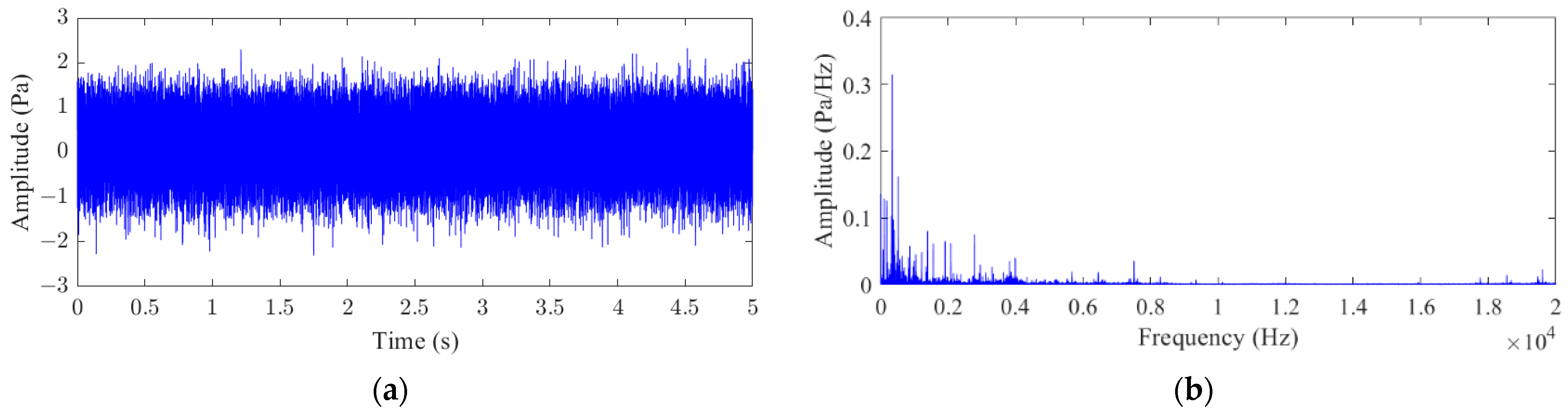
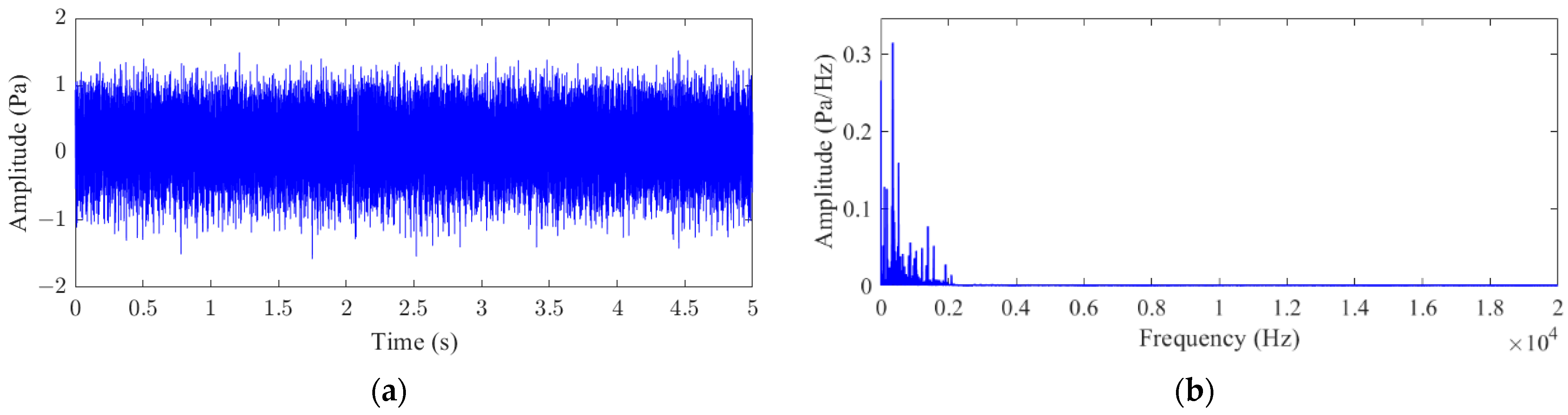
Data pre-processing: The original sound signal is decomposed into multiple chirped mode functions (CMFs) using ACMD. The CMFs with correlation coefficients greater than 0.3 are selected for signal reconstruction to remove the noise components and enhance the fault-related features in the signal. The reconstructed signal will be used for the subsequent feature extraction and fault identification.

3.

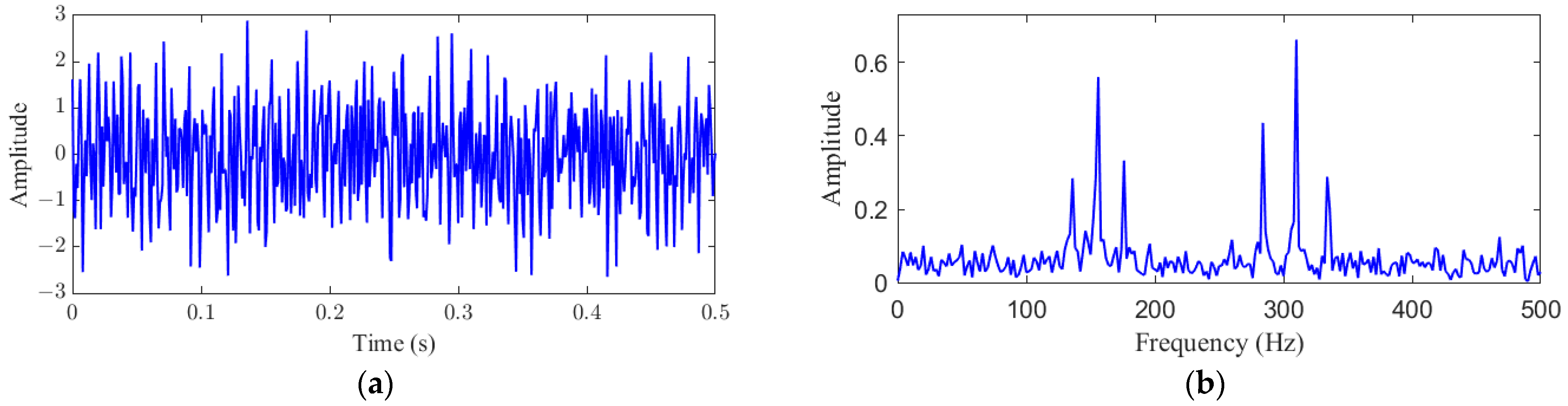
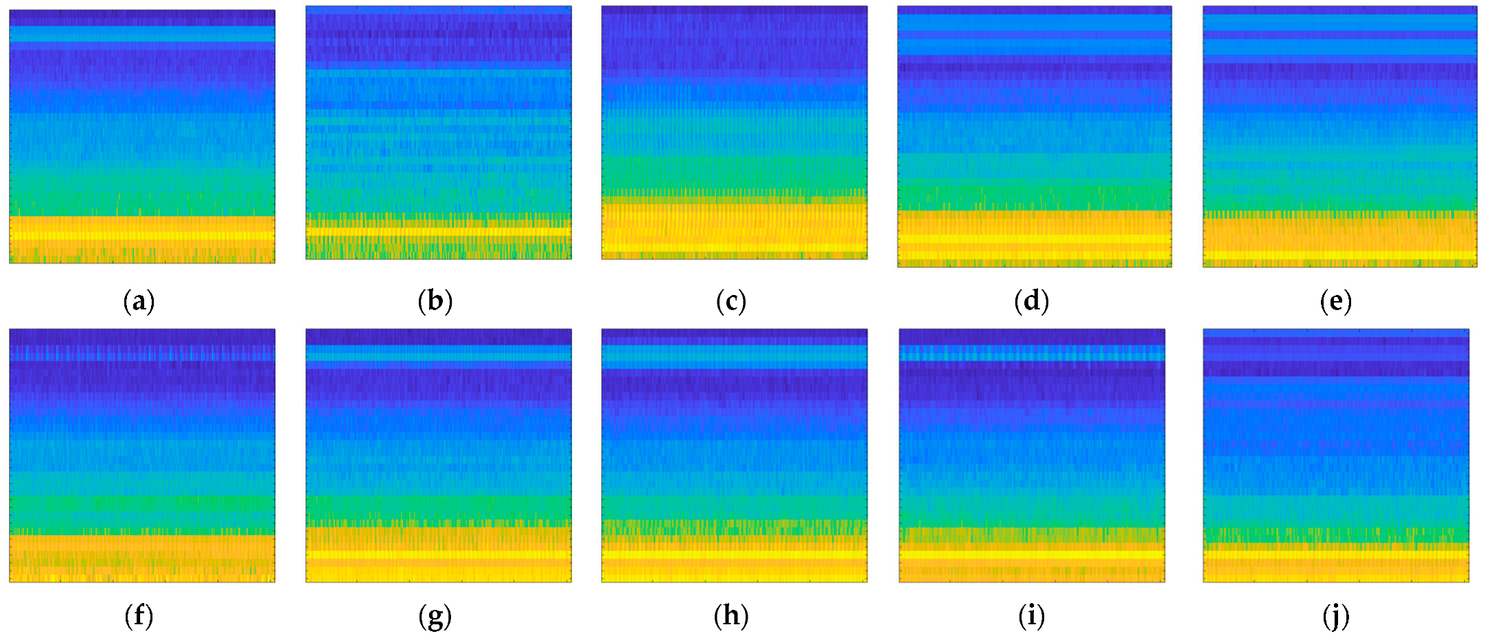
Feature extraction: The pre-processed sound signal is converted into a Mayer spectrogram. By simulating the auditory perception mechanism of the human ear, the Mayer spectrogram can effectively capture the key characteristics of the sound signal, which is particularly important in voiceprint recognition.

4.

Model training: Using the Mayer spectrogram obtained in the previous step as the input data, the MobileViT model is trained to recognize the different fault types of the pump. MobileViT is a lightweight model that combines a CNN and a Transformer for processing image data.

5.

Fault identification: The trained MobileViT model is used for the fault diagnosis of the constant pressure variable pump to achieve an accurate fault type determination.

Figure 7. Fault diagnosis process.

Figure 7. Fault diagnosis process.

4. Data Acquisition and Feature Set Construction

The effectiveness of a fault diagnosis heavily depends on the quality of the data and the robustness of the features extracted from it. This chapter provides a detailed overview of the setup process for the constant pressure variable pump fault simulation test system, including the configuration of the instruments used for data collection, the setting of the environmental conditions, and the methodology for constructing the acoustic fingerprint feature samples.

4.1. Experimental Setup

Figure 8 illustrates the test bench for simulating the faults in constant pressure variable pumps. Detailed information about the relevant components and their parameters can be found in

Table 1. Key parameters of main components of hydraulic pump.

Components	Model Number	Argument
Constant pressure variable pump	P08-B3-F-R-01	No-load displacement: 8 cm3/r
		Pressure regulation range: 3~21 MPa
		Speed range: 500~2000 r/min
Drive motor	C07-43BO	Rated power: 5.5 kW
		Rated speed: 1440 r/min
Sound level meter	AWA5661	Measuring range: 25~140 dB
		Sensitivity: 40 mV/Pa
		Frequency range: 10 Hz–16 kHz

. The test system is equipped with vibration sensors, flow sensors, pressure sensors, temperature sensors, and a sound level meter (the installation positions are shown in Figure 9). These sensors collect real-time data on the vibration signals, flow, pressure, temperature, and operational sounds of the constant pressure variable pumps during operation.

In order to ensure consistency between the simulated faults and the actual pump faults, this experiment refers to common fault characteristics in real fault situations and adopts fault injection technology to accurately simulate various fault scenarios (physical fault components are shown in Figure 10). This method enhances the similarity between the simulated faults and actual faults, thereby improving the accuracy of the experiment. Information regarding the normal working states and the various types of faults is shown in

Table 2. Failure mode and setting mode of constant pressure variable pump.

Serial Number	Failure Form	Injection Mode	Tag
1	Normal	—	F1
2	Slipper wear (light)	Using 80-grit sandpaper, the slipper pad was sanded until its mass decreased by 0.2 g, and it was appropriately biased during sanding.	F2
3	Slipper wear (heavy)	Using 40-grit sandpaper, the slipper pad was sanded until its mass decreased by 0.6 g, and it was appropriately biased during sanding.	F3
4	Loose boots (light)	Select a plunger with a certain degree of loose slipper pad, with a clearance of 0.24 mm.	F4
5	Loose boots (heavy)	Select a plunger with a certain degree of loose slipper pad, with a clearance of 0.48 mm.	F5
6	Plunger wear (light)	Using 180-grit sandpaper, the plunger was sanded until its mass was reduced by 0.15 g.	F6
7	Plunger wear (heavy)	Using 100-grit sandpaper, the plunger was sanded until its mass was reduced by 0.45 g.	F7
8	Inner race bearing fault	Using electrical discharge machining (EDM), a groove 1 mm wide and 1 mm deep was machined across the raceway of the inner ring of a rolling bearing, oriented perpendicular to the raceway direction.	F8
9	Outer race bearing fault	Using EDM, a groove 1 mm wide and 1 mm deep was machined across the raceway of the outer ring of a rolling bearing, oriented perpendicular to the raceway direction.	F9
10	Rolling element bearing fault	A pit with a diameter of 1 mm and a depth of 1 mm was machined on one of the rolling elements of a rolling bearing using EDM.	F10

.

According to the Nyquist theorem of signal processing, to avoid aliasing, the sampling frequency should be set to more than twice the highest frequency component in the sound signal. Given that the upper limit of human hearing is about 20 kHz, the sampling frequency for the experiment is set to 40 kHz to ensure accurate data capture. Additionally, the pump outlet temperature is controlled between 35 °C and 40 °C, the outlet pressure is set to 10 MPa, and the throttle valve is adjusted to regulate the pump outlet flow rate to 9 L per minute.

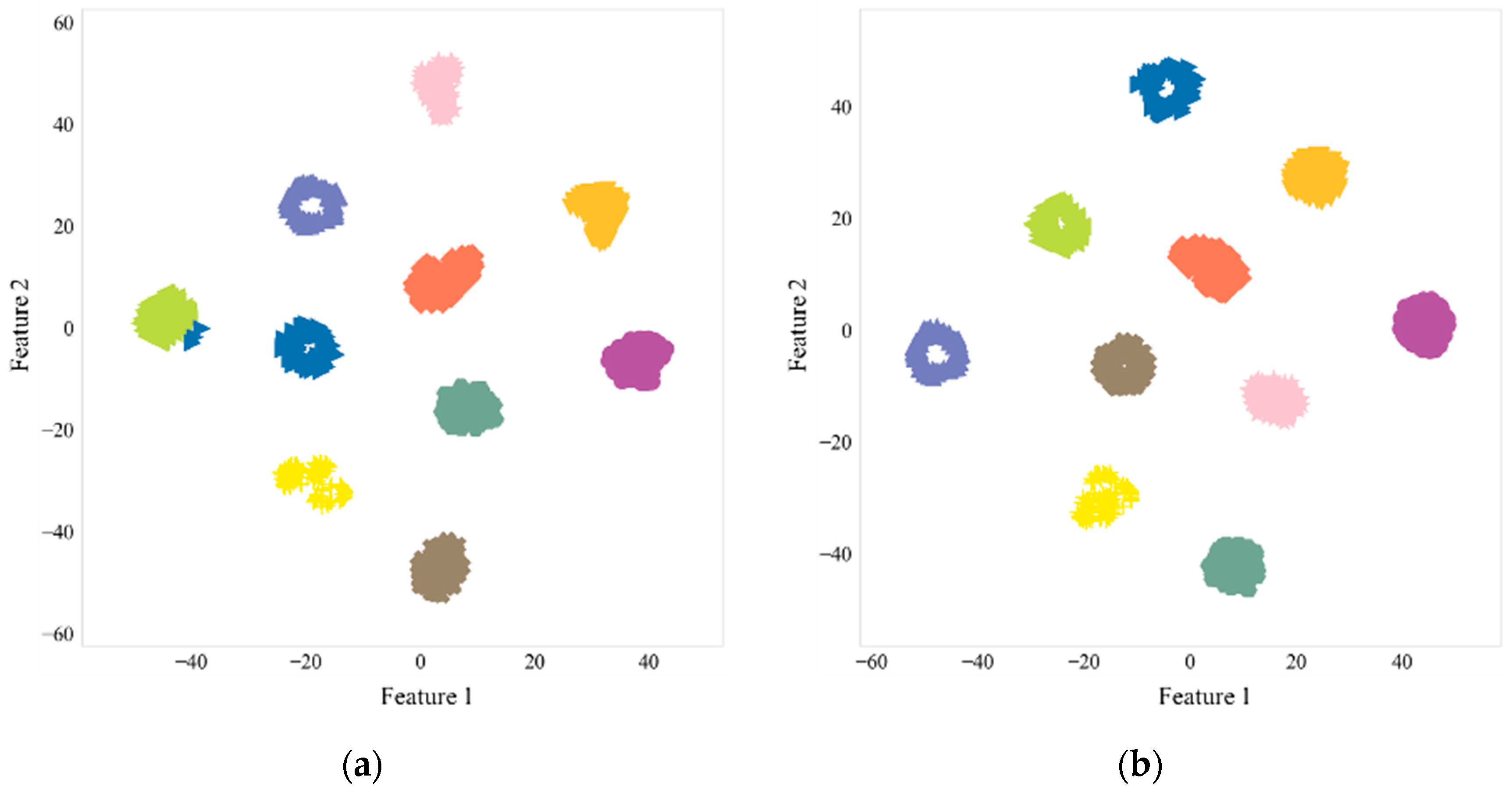
4.2. Mel Spectrum Sample Construction

The Mel spectrogram is a sound signal representation method designed based on human auditory perception mechanisms. It aims to provide a representation of sound signals that is closer to human auditory characteristics by simulating the ear’s varying sensitivity to different frequencies. In the field of audio signal processing, particularly in applications such as speech recognition, music information retrieval, and sound event detection, the Mel spectrogram is widely used because it expresses sound information in a manner that aligns closely with human auditory perception.

The generation process of the Mel spectrogram includes the following steps: Firstly, the sound signal is analyzed using the Short-Time Fourier Transform to obtain a spectrogram. Subsequently, the frequency values in the spectrogram are converted using the Mel scale to simulate the ear’s nonlinear perception of frequencies. Then, the energy within each Mel frequency band is log-transformed to reflect the logarithmic perception of sound intensity by the human ear. Finally, these processed data are displayed in the form of an image, where the horizontal axis represents time, the vertical axis represents the Mel frequencies, and the depth of color indicates the energy intensity at specific times and frequencies.

Figure 11 illustrates the process of constructing Mel spectrogram samples. For each type of fault, a sampling duration of 5 s is used, and the sampling is repeated three times to gather a sufficient amount of data. Given that the test rig’s motor operates at a rated speed of 1440 rpm, approximately 1667 samples are collected per shaft cycle. To ensure that each sampling frame contains more than one complete shaft cycle, the frame length is set to three times the number of samples per rotational cycle, which equates to 5120 samples per frame. Additionally, to ensure an adequate number of samples, the frame step is set to 1024. Thus, the entire dataset comprises 5700 Mel spectrogram images (570 for each fault type). For more details, please refer to

Table 3. Mel spectrum feature map data set construction.

Fault Type	Sample Size	Training Set	Test Set	Validation Set	Tag
Normal state	570	342	114	114	F1
Slipper wear (light)	570	342	114	114	F2
Slipper wear (heavy)	570	342	114	114	F3
Loose boots (light)	570	342	114	114	F4
Loose boots (heavy)	570	342	114	114	F5
Plunger wear (light)	570	342	114	114	F6
Plunger wear (heavy)	570	342	114	114	F7
Inner race bearing fault	570	342	114	114	F8
Outer race bearing fault	570	342	114	114	F9
Rolling element bearing fault	570	342	114	114	F10

. To fit the input size of the MobileViT model, the Mel spectrogram images are resized to 256 × 256. The training dataset, validation set, and test dataset are established by randomly splitting them into ratios of 60%, 20%, and 20%, respectively.

Figure 12 shows the time-domain waveform and spectrum of a sound signal from a plunger with mild wear. In the time domain, significant random fluctuations and prominent noise components are observable. Additionally, due to noise interference, the spectrum contains a large amount of high-frequency noise.

Figure 13 shows the time-domain waveform and spectrum of a sound signal after noise reduction and reconstruction using ACMD. The time-domain waveform after noise reduction shows significantly reduced random fluctuations and a narrower amplitude range, making the useful signal more clearly visible. This indicates that ACMD effectively removed most of the background noise, clarifying the signal’s waveform. Additionally, the spectrum after noise reduction shows a substantial reduction in high-frequency noise components.

Figure 14 shows the Mel spectrograms of sound signals from a constant pressure variable pump. It is evident that the Mel spectrograms of different fault types are distinctly different, especially within the frequency ranges of 0.7–0.9 kHz and 8–18 kHz. The significant energy differences between these Mel spectrograms provide crucial feature information for hydraulic pump fault diagnosis based on deep learning, helping to enhance the accuracy of the diagnostic model.

5. Fault Diagnosis Model Based on Mel-MobileVIT

This chapter primarily discusses the application of the Mel-MobileViT model for fault diagnosis in constant pressure variable pumps. Initially, it details the network structure of MobileViT and describes the modifications made to the network architecture to meet the specific input and output requirements of hydraulic pump fault diagnosis. Subsequently, the chapter analyzes the performance of the MobileViT model under various settings. Finally, it compares the fault diagnosis results of MobileViT with other lightweight networks.

5.1. The Network Structure of MobileViT

The MobileViT network structure is shown in

Table 4. MobileViT network architecture.

Layer		Output size	Repeat	Output Channels
				XXS	XS	S
	Image	256 × 256
Layer 1	Conv-3 × 3, ↓ 2 MV2	128 × 128	1 1	16 16	16 32	16 32
Layer 2	MV2, ↓ 2 MV2	64 × 64	1 2	24 24	48 48	64 64
Layer 3	MV2, ↓ 2 MobileViT block (L = 2)	32 × 32	1 1	48 48 (d = 64)	64 64 (d = 96)	96 96 (d = 144)
Layer 4	MV2, ↓ 2 MobileViT block (L = 4)	16 × 16	1 1	64 64 (d = 80)	80 80 (d = 120)	128 128 (d = 192)
Layer 5	MV2, ↓ 2 MobileViT block (L = 3) Conv-1 × 1	8 × 8	1 1 1	80 80 (d = 96) 320	96 96 (d = 144) 384	160 160 (d = 240) 640
Layer 6	Global pool Linear	1 × 1	1	10	10	10

. “Layer” indicates the modules traversed by each feature layer; “Output size” denotes the dimensions of each module’s output in the network; “Output channels” refers to the number of channels output after each feature layer; “L” represents the number of Transformer modules in the MVIT section; and the end of the network uses a global average pooling layer and a fully connected layer to integrate these features for the final classification task. The network offers three different configurations (mainly differing in the number of output feature map channels): MobileViT-S, MobileViT-XS, and MobileViT-XXS. Among them, S has the largest number of parameters, the deepest network, and the best performance, but requires the most resources. XXS has the smallest scale and is suitable for resource-limited environments [35].

In this paper, during the model training process, the batch size was set to 128. Additionally, the paper selected the Adam optimizer, which integrates momentum optimization and RMSProp features, to update model gradients during backpropagation. The initial learning rate for the optimizer was set at 0.001. Because the Adam optimizer adaptively adjusts the learning rate during training, it reduces dependency on learning rate schedulers. After multiple rounds of experiments, the number of iterations was finalized at 30 epochs. This setup not only ensures that the model is sufficiently trained but also prevents overfitting to the training set.

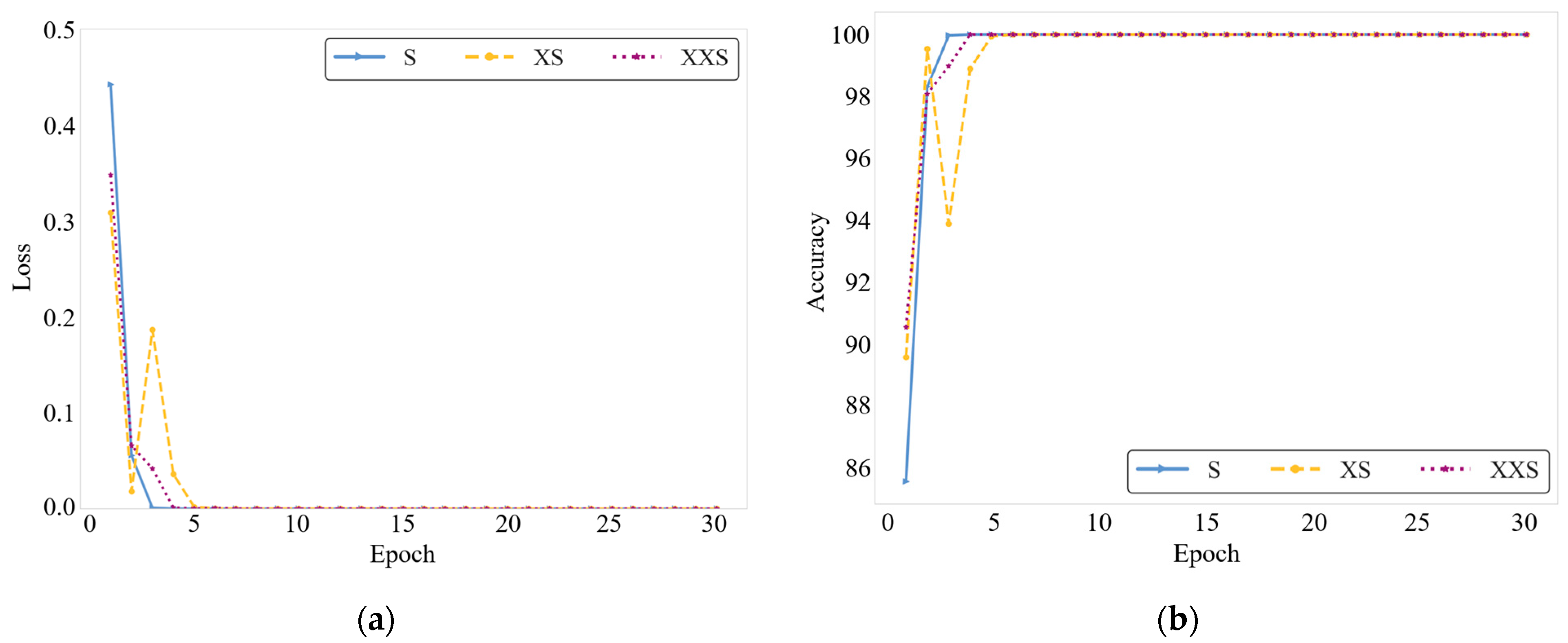
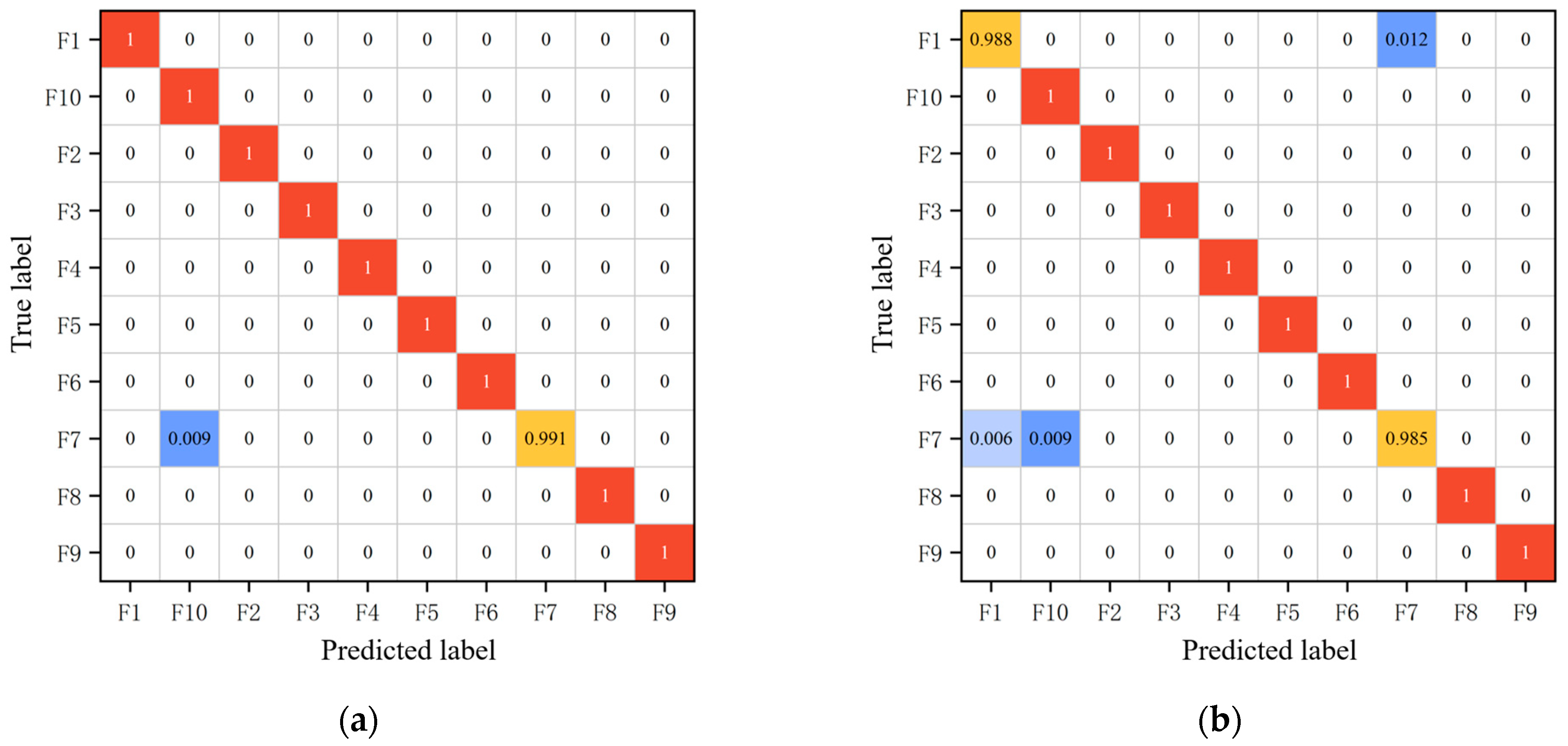
5.2. Result Analysis

The loss and accuracy curves for the three different configurations of the MobileViT model (S, XS, XXS) during the training process are shown in Figure 15. The results indicate that the S configuration performed the best in terms of loss reduction and accuracy improvement, demonstrating efficient learning capabilities and stability. Although XS and XXS also achieved high accuracy towards the end of training, XS exhibited significant loss fluctuations in the early stages of training, indicating weaker stability and generalization ability. However, from the fifth epoch onwards, the loss and accuracy curves for all configurations showed a relatively stable trend, with the loss values quickly decreasing to low levels and maintaining stability, while the accuracy rapidly improved to near 100% and remained high. These results demonstrate the efficiency and reliability of the MobileViT architecture.

Figure 16 shows the confusion matrices for the three configurations of the MobileViT model (S, XS, XXS). MobileViT-S achieved a recall rate of 100% for most samples, but had some misclassifications from category F7 to F10. For the XS configuration, the recall rates for categories F1 and F7 slightly decreased (to 0.988 and 0.985, respectively). The XXS configuration had recall rates of 0.986, 0.992, 0.999, and 0.991 for categories F1, F10, F4, and F7, respectively, possibly due to reduced feature extraction capability as a result of the smaller model size. The results indicate that as the model size decreases, the overall performance shows a slight decline, but still maintains high classification accuracy.

To further investigate the feature distribution, this study employs the t-distributed stochastic neighbor embedding (t-SNE) method for the dimensionality reduction and visualization of the features. The horizontal and vertical axes represent the two dimensions in the t-SNE embedding space, labeled as Component 1 and Component 2, respectively. Figure 17 illustrates the distribution of the test samples. From the figure, it can be observed that some F5-type features begin to cluster with F4-type features in the input feature distribution. After being processed by the local representation module (Layer 1), the features exhibit a more uniform distribution. Following processing by the global representation modules (Layers 2 to 5), the features of the same type form distinct clusters. Finally, after passing through the fusion module, the features of each fault type achieve well-defined clustering. These results demonstrate that the feature representations are progressively enhanced from local to global, leading to the effective spatial separation of fault types and significantly improved intra-class consistency.

To comprehensively analyze the performance of the proposed model, this study also examined the accuracy, computational complexity (measured in MFLOPs), number of parameters (Params), memory usage (MemR+W), and GPU processing efficiency on the validation set (Images/s) for each model (

Table 5. Performance comparison of three different configuration models of MobileViT.

Model	Acc. (%)	MFLOPs	Params/106	MemR+W (MB)	Images/s
MobileViT-S	99.91	1776.54	5	426.03	5.35
MobileViT-XS	99.73	922.82	2	335.89	31.26
MobileViT-XXS	99.59	341.54	1.01	136.90	75.95

and

Table 6. Performance comparison of three different configuration models of MobileViT (precision, recall, F1 score).

Class	MobileViT-S			MobileViT-XS			MobileViT-XXS
	Precision	Recall	F1 Score	Precision	Recall	F1 Score	Precision	Recall	F1 Score
F1	1	1	1	0.994	0.988	0.991	1	0.986	0.993
F10	0.991	1	0.996	0.991	1	0.996	0.977	0.992	0.985
F2	1	1	1	1	1	1	1	1	1
F3	1	1	1	1	1	1	1	1	1
F4	1	1	1	1	1	1	0.992	0.991	0.991
F5	1	1	1	1	1	1	0.998	1	0.999
F6	1	1	1	1	1	1	1	1	1
F7	1	0.991	0.995	0.988	0.985	0.986	0.991	0.99	0.991
F8	1	1	1	1	1	1	1	1	1
F9	1	1	1	1	1	1	1	1	1

).

In terms of accuracy, as the model size decreases, the accuracies of the S, XS, and XXS models drop, yet remain high at 99.91%, 99.73%, and 99.59%, respectively. Regarding computational resource consumption, the computational complexity of the XXS model is only 341.54 MFLOPs, significantly lower than that of S and XS. In terms of the number of parameters, the XXS configuration has only half as many parameters as XS and one-fifth as many as S, greatly reducing the model’s complexity. This helps decrease the training and inference time, while also lowering the storage requirements. Concerning memory usage, the XXS configuration only requires 136.90 MB, far less than the 426.03 MB required by the S configuration, making it more suitable for deployment on memory-constrained devices.

From a GPU processing speed perspective, XXS also performs excellently, processing up to 75.95 images per second, which represents an approximate increase of 1319.63% compared to the S configuration. Considering these metrics, although the MobileViT model experiences a slight decrease in accuracy with reduced size, the reduction is relatively small. Particularly, the XXS model, while maintaining a high accuracy, significantly reduces the demand for computational resources. Overall, despite a minor decrease in accuracy as the MobileViT model size is reduced, its overall performance remains outstanding, especially in environments with limited computational resources, where the XXS model demonstrates high practical value.

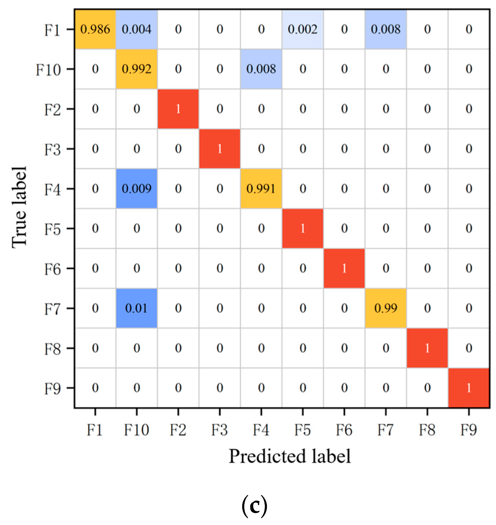
5.3. Comparative Study of Different Models

To verify the effectiveness of the proposed lightweight network MobileViT, this paper compares it with two derivatives of MobileNet: MobileNetV1 and MobileNetV2. These models are lightweight convolutional neural networks developed by Google. MobileNetV1 reduces computational demands through depthwise separable convolutions, while MobileNetV2 builds on this by introducing linear bottleneck layers and an inverted residual structure. This not only enhances the network’s classification accuracy and processing speed but also makes it highly suitable for real-time image processing tasks on devices with limited computational resources [36]. MobileNetV1 and MobileNetV2 focus on reducing model size and enhancing efficiency through improvements in convolutional structures. In contrast, MobileViT integrates convolutional and Transformer architectures, aiming to provide deeper contextual understanding and processing capabilities while maintaining a lightweight structure.

Figure 18 shows the confusion matrices for three lightweight networks (V1, V2, XXS) when processing the Mel spectrogram data from constant pressure variable pumps. Detailed performance data for the models can be found in

Table 7. The comparison of the performance of the MobileViT and MobileNet models.

Model	Acc. (%)	MFLOPs	Params/106	MemR+W (MB)	Images/s
MobileViT-XXS	99.59	341.54	1.01	136.90	75.95
MobileNetV2	99.72	426.07	2.23	163.76	100.76
MobileNetV1	98.10	767.86	3.21	208.91	118.21

and

Table 8. The comparison of the performance of the MobileViT and MobileNet models (precision, recall, and F1 score).

Class	MobileViT-XXS			MobileNetV1			MobileNetV2
	Precision	Recall	F1 Score	Precision	Recall	F1 Score	Precision	Recall	F1 Score
F1	1	0.986	0.993	1	0.885	0.939	0.994	1	0.997
F10	0.977	0.992	0.985	0.991	1	0.996	0.988	0.99	0.989
F2	1	1	1	0.862	1	0.926	1	1	1
F3	1	1	1	1	1	1	1	1	1
F4	0.992	0.991	0.991	1	0.991	0.995	1	1	1
F5	0.998	1	0.999	1	0.991	0.995	1	1	1
F6	1	1	1	1	1	1	1	1	1
F7	0.991	0.99	0.991	1	0.947	0.973	0.99	0.982	0.986
F8	1	1	1	1	1	1	1	1	1
F9	1	1	1	0.983	1	0.991	1	1	1

. The results indicate that MobileNetV2 performs the best in classification tasks, with the highest accuracy of 99.72%. However, MobileViT-XXS follows closely with an accuracy of 99.59%. Although slightly lower than that of MobileNetV2, the small gap still demonstrates its excellent classification performance. MobileViT-XXS excels in the computational resource requirements (341.54 MFLOPs) and the number of parameters (1.01 million), significantly outperforming MobileNetV2 and MobileNetV1. Additionally, MobileViT-XXS has the lowest memory consumption at 136.90 MB, indicating its advantage in resource-limited environments. Although MobileNetV1 processes images the fastest (118.21 images per second), the processing speed of MobileViT-XXS (75.95 images per second) also meets the needs of many practical applications.

In summary, the fault diagnosis method for constant pressure variable pumps proposed in this study fully considers the needs of applications in resource-constrained environments. As a result, the architecture not only demonstrates high accuracy but also significant practicality in real-world applications. This provides an optimal solution for hydraulic pump fault diagnosis, balancing precise identification with low computational costs.

The computational experiments in this study were conducted using a system equipped with an Intel Core i7-11800H processor, an NVIDIA GeForce RTX 3060 Laptop GPU, and 32 GB of RAM, purchased from Qinhuangdao, Hebei Province, China. The development environment included Matlab 2023a, Python 3.6.12, scikit-learn 0.24.2, and TensorFlow-GPU 2.6.0.

6. Conclusions

This paper combines deep learning and signal processing technologies to propose an intelligent fault diagnosis method for hydraulic pumps based on sound signals. It employs a lightweight convolutional neural network to classify the acoustic patterns of different fault states. Experimental validation shows that this method not only enhances the accuracy of fault diagnosis based on sound signals but also effectively reduces the demand for hardware resources, offering a new technical approach to the intelligent maintenance of hydraulic pumps. Conclusions are as follows:

1.

This paper utilizes ACMD to adaptively extract the instantaneous frequency of sound signals, separate various modal components, and reconstruct signals using highly correlated modes based on the Pearson correlation coefficient for noise reduction. It also compares well with noise reduction algorithms like EMD and VMD. The results show that ACMD is more effective in reducing noise levels when processing the sound signals from hydraulic pumps.

2.

This paper applies the MobileViT network to fault diagnosis in constant pressure variable pumps and compares it with existing lightweight deep learning models. The results demonstrate that MobileViT not only maintains high recognition accuracy, but also significantly reduces the model’s computational complexity and parameter requirements, thereby enhancing the diagnostic efficiency.

3.

The method proposed in this paper is non-invasive, employing sound sensors which, compared to other types of sensors, offer advantages such as easy installation, low maintenance costs, and no disruption to normal equipment operation. These benefits significantly enhance the applicability and reliability of the fault diagnosis system.

4.

Although the model in this paper performs well under specific experimental conditions, the actual effect on hydraulic pumps under different working conditions may be different. In practical applications, it may be necessary to further collect more training data, covering different equipment models and working conditions, to improve the versatility and adaptability of the model.

References

1. Zhang, Q.; Kong, X.; Yu, B.; Ba, K.; Jin, Z.; Kang, Y. Review and Development Trend of Digital Hydraulic Technology. Appl. Sci. 2020, 10, 579. [Google Scholar] [CrossRef]
2. Yang, Y.; Ding, L.; Xiao, J.; Fang, G.; Li, J. Current Status and Applications for Hydraulic Pump Fault Diagnosis: A Review. Sensors 2022, 22, 9714. [Google Scholar] [CrossRef] [PubMed]
3. Kong, X.; Cai, B.; Liu, Y.; Zhu, H.; Liu, Y.; Shao, H.; Yang, C.; Li, H.; Mo, T. Optimal Sensor Placement Methodology of Hydraulic Control System for Fault Diagnosis. Mech. Syst. Signal Process. 2022, 174, 109069. [Google Scholar] [CrossRef]
4. Ye, S.; Zhang, J.; Xu, B.; Zhu, S.; Xiang, J.; Tang, H. Theoretical Investigation of the Contributions of the Excitation Forces to the Vibration of an Axial Piston Pump. Mech. Syst. Signal Process. 2019, 129, 201–217. [Google Scholar] [CrossRef]
5. Shan, Z.; Li, Z.; Zhang, X.; Huang, Y.; Li, Y.; Liu, C.; Zhang, X. Health Status Assessment of Hydraulic Pumps Based on Multi-Sensor Information Fusion and Multi-Grained Cascade Forest Model. China Mech. Eng. 2021, 32, 2374–2382. [Google Scholar] [CrossRef]
6. Wang, S.; Xiang, J.; Zhong, Y.; Tang, H. A Data Indicator-Based Deep Belief Networks to Detect Multiple Faults in Axial Piston Pumps. Mech. Syst. Signal Process. 2018, 112, 154–170. [Google Scholar] [CrossRef]
7. Ye, S.; Zhang, J.; Xu, B.; Hou, L.; Xiang, J.; Tang, H. A Theoretical Dynamic Model to Study the Vibration Response Characteristics of an Axial Piston Pump. Mech. Syst. Signal Process. 2021, 150, 107237. [Google Scholar] [CrossRef]
8. Toutountzakis, T.; Tan, C.K.; Mba, D. Application of Acoustic Emission to Seeded Gear Fault Detection. NDT E Int. 2005, 38, 27–36. [Google Scholar] [CrossRef]
9. Abdul, Z.K.; Al-Talabani, A.K. Mel Frequency Cepstral Coefficient and Its Applications: A Review. IEEE Access 2022, 10, 122136–122158. [Google Scholar] [CrossRef]
10. Glowacz, A.; Glowacz, W.; Glowacz, Z.; Kozik, J. Early Fault Diagnosis of Bearing and Stator Faults of the Single-Phase Induction Motor Using Acoustic Signals. Measurement 2018, 113, 1–9. [Google Scholar] [CrossRef]
11. Tang, L.; Wu, X.; Wang, D.; Liu, X. A Comparative Experimental Study of Vibration and Acoustic Emission on Fault Diagnosis of Low-Speed Bearing. IEEE Trans. Instrum. Meas. 2023, 72, 1–11. [Google Scholar] [CrossRef]
12. Hou, D.; Qi, H.; Wang, C.; Han, D. High-Speed Train Wheel Set Bearing Fault Diagnosis and Prognostics: Fingerprint Feature Recognition Method Based on Acoustic Emission. Mech. Syst. Signal Process. 2022, 171, 108947. [Google Scholar] [CrossRef]
13. Elasha, F.; Greaves, M.; Mba, D. Planetary Bearing Defect Detection in a Commercial Helicopter Main Gearbox with Vibration and Acoustic Emission. Struct. Health Monit. 2018, 17, 1192–1212. [Google Scholar] [CrossRef]
14. Pham, M.T.; Kim, J.-M.; Kim, C.H. Rolling Bearing Fault Diagnosis Based on Improved GAN and 2-D Representation of Acoustic Emission Signals. IEEE Access 2022, 10, 78056–78069. [Google Scholar] [CrossRef]
15. Tang, S.; Zhu, Y.; Yuan, S. Intelligent Fault Diagnosis of Hydraulic Piston Pump Based on Deep Learning and Bayesian Optimization. ISA Trans. 2022, 129, 555–563. [Google Scholar] [CrossRef]
16. Shan, S.; Liu, J.; Wu, S.; Shao, Y.; Li, H. A Motor Bearing Fault Voiceprint Recognition Method Based on Mel-CNN Model. Measurement 2023, 207, 112408. [Google Scholar] [CrossRef]
17. Tran, T.; Lundgren, J. Drill Fault Diagnosis Based on the Scalogram and Mel Spectrogram of Sound Signals Using Artificial Intelligence. IEEE Access 2020, 8, 203655–203666. [Google Scholar] [CrossRef]
18. Islam, M.M.M.; Kim, J.-M. Automated Bearing Fault Diagnosis Scheme Using 2D Representation of Wavelet Packet Transform and Deep Convolutional Neural Network. Comput. Ind. 2019, 106, 142–153. [Google Scholar] [CrossRef]
19. Kumar, A.; Gandhi, C.P.; Zhou, Y.; Kumar, R.; Xiang, J. Improved Deep Convolution Neural Network (CNN) for the Identification of Defects in the Centrifugal Pump Using Acoustic Images. Appl. Acoust. 2020, 167, 107399. [Google Scholar] [CrossRef]
20. Ji, S.; Han, B.; Zhang, Z.; Wang, J.; Lu, B.; Yang, J.; Jiang, X. Parallel Sparse Filtering for Intelligent Fault Diagnosis Using Acoustic Signal Processing. Neurocomputing 2021, 462, 466–477. [Google Scholar] [CrossRef]
21. Shao, Y.; Chao, Q.; Xia, P.; Liu, C. Fault Severity Recognition in Axial Piston Pumps Using Attention-Based Adversarial Discriminative Domain Adaptation Neural Network. Phys. Scr. 2024, 99, 056009. [Google Scholar] [CrossRef]
22. Huang, W.; Shen, Z.; Huang, N.E.; Fung, Y.C. Engineering Analysis of Biological Variables: An Example of Blood Pressure over 1 Day. Proc. Natl. Acad. Sci. USA 1998, 95, 4816–4821. [Google Scholar] [CrossRef] [PubMed]
23. Huang, N.E. Review of Empirical Mode Decomposition. In Wavelet Applications VIII; Szu, H.H., Donoho, D.L., Lohmann, A.W., Campbell, W.J., Buss, J.R., Eds.; Spie-Int Soc Optical Engineering: Bellingham, WA, USA, 2001; Volume 4391, pp. 71–80. [Google Scholar]
24. Dragomiretskiy, K.; Zosso, D. Variational Mode Decomposition. IEEE Trans. Signal Process. 2014, 62, 531–544. [Google Scholar] [CrossRef]
25. Chen, S.; Yang, Y.; Peng, Z.; Wang, S.; Zhang, W.; Chen, X. Detection of Rub-Impact Fault for Rotor-Stator Systems: A Novel Method Based on Adaptive Chirp Mode Decomposition. J. Sound Vibr. 2019, 440, 83–99. [Google Scholar] [CrossRef]
26. Chen, S.; Yang, Y.; Peng, Z.; Dong, X.; Zhang, W.; Meng, G. Adaptive Chirp Mode Pursuit: Algorithm and Applications. Mech. Syst. Signal Proc. 2019, 116, 566–584. [Google Scholar] [CrossRef]
27. Bhatt, D.; Patel, C.; Talsania, H.; Patel, J.; Vaghela, R.; Pandya, S.; Modi, K.; Ghayvat, H. CNN Variants for Computer Vision: History, Architecture, Application, Challenges and Future Scope. Electronics 2021, 10, 2470. [Google Scholar] [CrossRef]
28. Liu, Y.; Pu, H.; Sun, D.-W. Efficient Extraction of Deep Image Features Using Convolutional Neural Network (CNN) for Applications in Detecting and Analysing Complex Food Matrices. Trends Food Sci. Technol. 2021, 113, 193–204. [Google Scholar] [CrossRef]
29. Yao, Q.; Wang, R.; Fan, X.; Liu, J.; Li, Y. Multi-Class Arrhythmia Detection from 12-Lead Varied-Length ECG Using Attention-Based Time-Incremental Convolutional Neural Network. Inf. Fusion 2020, 53, 174–182. [Google Scholar] [CrossRef]
30. Tang, S.; Zhu, Y.; Yuan, S. An Improved Convolutional Neural Network with an Ad Learning Rate towards Multi-Signal Fault Diagnosis of Hydraulic Piston Pump. Adv. Eng. Inform. 2021, 50, 101406. [Google Scholar] [CrossRef]
31. Khan, A.; Sohail, A.; Zahoora, U.; Qureshi, A.S. A Survey of the Recent Architectures of Deep Convolutional Neural Networks. Artif. Intell. Rev. 2020, 53, 5455–5516. [Google Scholar] [CrossRef]
32. Yang, H.; Zhang, Y.; Yin, C.; Ding, W. Ultra-Lightweight CNN Design Based on Neural Architecture Search and Knowledge Distillation: A Novel Method to Build the Automatic Recognition Model of Space Target ISAR Images. Def. Technol. 2022, 18, 1073–1095. [Google Scholar] [CrossRef]
33. Zhong, H.; Lv, Y.; Yuan, R.; Yang, D. Bearing Fault Diagnosis Using Transfer Learning and Self-Attention Ensemble Lightweight Convolutional Neural Network. Neurocomputing 2022, 501, 765–777. [Google Scholar] [CrossRef]
34. Ruan, D.; Han, J.; Yan, J.; Gühmann, C. Light Convolutional Neural Network by Neural Architecture Search and Model Pruning for Bearing Fault Diagnosis and Remaining Useful Life Prediction. Sci. Rep. 2023, 13, 5484. [Google Scholar] [CrossRef] [PubMed]
35. Mehta, S.; Rastegari, M. MobileViT: Light-Weight, General-Purpose, and Mobile-Friendly Vision Transformer. arXiv 2021. [Google Scholar] [CrossRef]
36. Kumar, A.; Sharma, A.; Bharti, V.; Singh, A.K.; Singh, S.K.; Saxena, S. MobiHisNet: A Lightweight CNN in Mobile Edge Computing for Histopathological Image Classification. IEEE Internet Things J. 2021, 8, 17778–17789. [Google Scholar] [CrossRef]
Figure 1. Convolutional neural network structure.
Jmse 12 01677 g001
Figure 3. The simulated signal includes complex time-varying signals and noise. s ( t ) : (a) time-domain waveform; (b) spectrum.
Jmse 12 01677 g003
Figure 4. ACMD algorithm results (blue: true; red: ACMD): (a) time-domain waveform comparison; (b) frequency comparison.
Jmse 12 01677 g004
Figure 5. The time-frequency distribution of the simulated signal: (a) CWT; (b) STFT; (c) ACMD.
Jmse 12 01677 g005
Figure 6. The processing results of the proposed simulation signal by the EMD, VMD, and ACMD algorithms: (a) the spectrum of the original signal; (b) the spectrum of the ACMD modal components; (c) the spectrum of the reconstructed signal from EMD; (d) the spectrum of the reconstructed signal from VMD (K = 8); (e) the EMD component spectrum; and (f) the VMD component spectrum.
Jmse 12 01677 g006aJmse 12 01677 g006b
Figure 8. The schematic diagram of the hydraulic system of the constant pressure variable pump fault simulation test bench.
Jmse 12 01677 g008
Figure 9. Sensor installation position of constant pressure variable pump fault simulation test system.
Jmse 12 01677 g009
Figure 10. Physical images of constant pressure variable pump components with faults: (a) slipper pad wear (normal, light, severe); (b) loose slipper (normal, light, severe); (c) plunger wear (normal, light, severe); (d) inner race bearing fault; (e) outer race bearing fault; (f) rolling element bearing fault.
Jmse 12 01677 g010
Figure 11. Mel spectrogram sample construction process.
Jmse 12 01677 g011
Figure 12. Acoustic signal of plunger failure: (a) fault signal time domain; (b) spectrogram.
Jmse 12 01677 g012
Figure 13. Sound signals of plunger fault after ACMD processing: (a) reconstructed signal time domain; (b) spectrum of the reconstructed signal.
Jmse 12 01677 g013
Figure 14. Mel spectrograms of hydraulic pump under various fault conditions: (a) normal; (b) slipper boots (light); (c) slipper boots (heavy); (d) loose boots (light); (e) loose boots (heavy); (f) plunger (light); (g) plunger (heavy); (h) bearing inner ring; (i) bearing outer ring; (j) rolling element.
Jmse 12 01677 g014
Figure 15. Training loss and accuracy curves for Mel-MobileViT: (a) training loss; (b) training accuracy.
Jmse 12 01677 g015
Figure 16. Confusion matrices for different configurations of MobileViT: (a) S; (b) XS; (c) XXS.
Jmse 12 01677 g016aJmse 12 01677 g016b
Figure 17. Clustering effect of each layer of network: (a) Input data; (b) Layer 1; (c) Layer 5; (d) Layer 6.
Jmse 12 01677 g017aJmse 12 01677 g017b
Figure 18. Confusion matrices: (a) MobileViT-XXS; (b) MobileNetV1; (c) MobileNetV2.
Jmse 12 01677 g018