Abstract
As the nonlinear and coupling characteristics of autonomous underwater vehicles (AUVs) are the challenges for motion modeling, the nonparametric identification method is proposed based on dung beetle optimization (DBO) and deep temporal convolutional networks (DTCNs). First, the improved wavelet threshold is utilized to select the optimal threshold and wavelet basis functions, and the raw model test data are denoising. Second, the bidirectional temporal convolutional networks, the bidirectional gated recurrent unit, and the attention mechanism are used to achieve the nonlinear nonparametric model of the AUV motion. And the hyperparameters are optimized by the DBO. Finally, the lazy-search-based path planning and the line-of-sight-based path following control are used for the proposed AUV model. The simulation shows that the prediction accuracy of the DBO-DTCN is better than other artificial intelligence methods and mechanical models, and the path following of AUV is feasible. The methods proposed in this paper can provide an effective strategy for AUV modeling, searching, and rescue cruising.
1. Introduction
In recent years, with the development of autonomous technology, marine vehicles have developed rapidly. Marine vehicles are divided into remotely operated underwater vehicles, manned submersibles, and autonomous underwater vehicles (AUVs). AUVs have mobility and autonomy without human intervention, play an important role in a variety of underwater activities, such as ocean observation, offshore industry, and naval defense, and are also a kind of robot for underwater hazardous environments [1], which can be used in submarine surveys, ocean search and rescue (SAR), etc. [2]. Compared with manual SAR, it can not only obtain real-time information through high-definition cameras and sensors to assist SAR personnel to rapidly locate the target but also prevent SAR personnel from directly facing the dangers. However, the further improvement of collision avoidance and autonomous navigation technology is still the challenge for underwater vehicles, and the motion model of underwater vehicles is particularly important.
Traditional methods used for motion modeling of surface vessels include support vector machines (SVM) [3], Random Forests (RF) [4], and local weighting [5]. Commonly, system identification [6] is the standard validation process of machine learning and prediction performed on a complete dataset of training and validation [7]. However, the combination of explosion problems is a challenge for system identification. Ship motion modeling based on Gaussian process regression (GP) [8] and Grey Wolf Optimization-SVR (GWO-SVR) [9] was developed to identify the nonlinear mathematical model of ship motion. Machine learning on the ship parameter identification can be heuristic algorithms to obtain the best parameters to solve the combination of explosion problems [10]. However, the hyperparameters of machine learning algorithms are hard to set, and colony algorithms [11,12].
For noise interference in the experimental data of the ship model, the noise processing has become an indispensable step before the model training [3]. In the ship research field, Shen et al. [13] used the Improved Complete Ensemble Empirical Mode Decomposition with Adaptive Noise (ICEEMDAN) to eliminate the noise caused by environmental factors and solve the data noise problem. Zhang et al. [14] added wave noise to the simulation data and used the wavelet threshold method to reduce the noise-containing data, and the denoised data verified the generalization of the wavelet threshold compared with the original data. However, the above study focuses on surface ship motion modeling and is not applied to nonlinear and strongly coupled AUV motion.
With the rapid development of artificial intelligence technology, deep reinforcement learning is now being used for ship motion system identification [15]. The method of neural networks of three degrees of freedom (DOF) model of a ship is able to obtain the nonlinear characteristics of the motion but needs a long training time [16]. Once the attention mechanism and the long and short-term memory (LSTM) networks [17], reference model [18], and Gate Recurrent Unit (GRU) [19] have been used, the better generalizability and nonlinearity will be achieved. The LSTM, GRU, and temporal convolutional neural networks (TCN) are the alternative methods for AUV. However, AUV is much different from ships for much more DOF and motion capability.
AUV motion control is the next step of motion modeling. Deep Reinforcement Learning (DRL) is a feasible method for AUV control [20], and AUV autonomy is the key to its applicability in complex tasks [21]. However, for the problem of relatively limited AUV coverage path planning [22], the constrained line-of-sight (LOS) path-following control strategy has been widely used [23]. For the path planning problem of AUV [24], the hierarchical approach [25], like A* and APF (AplusPF) [26], are feasible methods, and the colony optimization like ant colony optimization (ACO) [27] and particle swarm optimization (PSO) can make the hierarchical approach much more efficient. For this reason, the AUV environment is a challenge for path planning [28], the rapid exploration [29] can solve the unknown information, and the particle swarm [30] can address the ocean current and seabed topography. Thus, this research makes it possible for the AUV model test in path planning and the following task.
There are two key challenges in the motion modeling of AUV: nonlinearity and coupling [31]. AUV exhibits significant nonlinearity during maneuvers with large rudder angles, which increases the difficulty and uncertainty of modeling. If the model lacks accuracy, prediction errors in the AUV’s motion will progressively increase over time [32]. Furthermore, the coupling between velocity and angular velocity in AUV motion can further exacerbate prediction errors during maneuvers.
There are Computational Fluid Dynamics (CFD), Experimental Fluid Dynamics EFD and system identification for AUV motion modeling. First, using CFD methods to calculate the hydrodynamics of AUV is a current research hotspot. While CFD methods [33] provide accurate hydrodynamic analysis, they are time-consuming and require recalculation for different operating conditions, which may limit their efficiency and flexibility in practical applications [34]. Secondly, EFD methods are relatively less utilized in AUV research, partly due to the high precision requirements for experimental conditions, such as maneuvering basin testing environments. Moreover, the construction of scaled AUV models is costly, making large-scale experimental studies more challenging [35]. Given these challenges, this paper proposes using an identification method for studying AUV motion. The identification method is highly adaptable, allowing for analysis and research under various conditions without the extensive computational resources required by CFD methods or the high-cost experimental setups needed for EFD methods. Consequently, the identification method demonstrates greater practicality and flexibility in complex and variable operating conditions [36].
To address the nonlinearity and coupling problems, firstly, this paper proposes a deep learning-based approach to capture the complex dynamic behavior of AUV by capture their nonlinear motion characteristics. Specifically, six deep neural networks are employed to establish regression models corresponding to the 6-DOF of the AUV, addressing the coupling problem. Secondly, the paper utilizes the AUV model test, which is rare in other AUV identification studies [37], allowing for a more realistic environment. For the realistic environment noise, an improved wavelet threshold function is employed to enhance the filtering performance of model test data, avoiding white noise commonly used in the literature [38].
The main contributions of this paper are as follows:
- (1)
- Improved threshold function and suitable wavelet basis function are proposed for noise reduction of noise-containing data to make AUV motion model training data more reliable.
- (2)
- Deep-TCN (DTCN) model is proposed for motion nonparametric identification of AUV to capture the nonlinearity and coupling of motion.
- (3)
- Propose the dung beetle optimization (DBO) algorithm to find the optimal hyperparameters of the nonparameter model to ensure the authenticity and reliability of the nonparameter AUV model.
- (4)
- Propose the practical application of the AUV model by constructing a 3-D ocean model, using a algorithm for path planning, and applying the LOS guidance for path-following control.
In this paper, Section 2 utilizes the wavelet threshold method for noise reduction processing of ship model test data. Section 3 proposes the AUV motion model and constructs the DTCN nonparametric model. Section 4 optimizes the parameters of the constructed nonparametric model using the DBO algorithm. Section 5 carries out the model identification process. Section 6 performs path planning and following for AUV SAR. Section 7 is the conclusion.
2. Ship Model Test Data Noise Reduction
In this section, the wavelet threshold method algorithm [39] is selected for the presence of noise in the AUV ship model data. AUV ship model data acquisition includes (surge, sway, heave, rolling velocity, pitching velocity, and yawing velocity) and control variable (vertical rudder, horizontal rudder), etc. Due to the large noise interference in the collected data from the linear velocity of the AUV, noise reduction in the linear velocity data is needed to improve the quality of the training data, thus improving the performance and generalization ability of the model.
2.1. Wavelet Threshold Model
The mathematical expression for the linear velocity signal with noise in the AUV ship model data is Equation (1):
where is the noisy linear velocity signal, is the noisy signal, and is the pure signal. The essence of denoising the AUV ship model data is to obtain a relatively pure signal from the noisy signal such that it is an optimal approximation of under some error estimation.
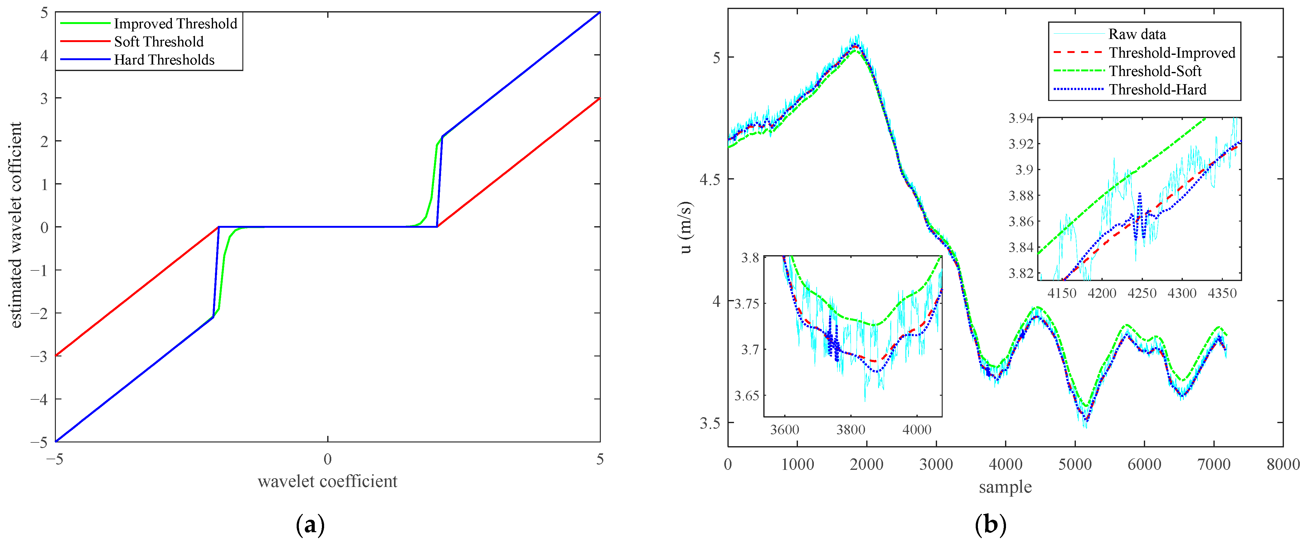
The key to wavelet threshold denoising is the choice of threshold function and wavelet basis function. Traditional threshold functions [40] include hard and soft thresholds.
Hard threshold function is Equation (2):
Soft Threshold function is Equation (3):
where sgn is the sign function, threshold is taken as , is the wavelet coefficients, and is the estimated wavelet coefficients.
When the ZigZag test and the Turning test are conducted, the change in rudder angle is a step change, which causes the gradual change in velocity and acceleration. Therefore, both hard and soft thresholds are not suitable for noise processing of ship motion data, and we adopt an improved threshold function.
Improved threshold function [41] is Equation (4):
where and are adjustment parameters, takes the value of any real number, is between , this paper chooses the parameters are 2 and 0.5 respectively. Three threshold functions are compared, as shown in Figure 1. The improved threshold function conforms to the gradual change of linear velocity after the change in the AUV rudder angle and is able to provide better noise reduction for the linear velocity data. According to the results in Figure 1b, it can be found that the result of the hard threshold function (blue dotted line) has some oscillations at 3750 and 4250 samples. Because the hard threshold function is discontinuous in Figure 1a. While the result of the soft threshold function (green dashed line) will lead to deviation from the raw data. However, the improved threshold avoids these problems in the hard and soft threshold functions.
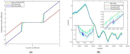
Figure 1.
Threshold functions comparison and application to surge velocity filtering. (a) Different threshold curves; (b) the result of filtering by different threshold functions.
Different choices of wavelet basis functions produce different effects on the noise reduction in the data. The optimal wavelet basis functions and optimal decomposition layers are derived by comparing the data. In this paper, several common basis functions, including haar, db3, bior2.4, coif3, sym2, dmey, and rbio2.4, are used to select the optimal wavelet basis function by comparison. The optimal number of stratifications uses the idea of control variables and different stratifications of the selected wavelet basis functions to determine the optimal number of stratifications.
2.2. Noise Reduction Study Case
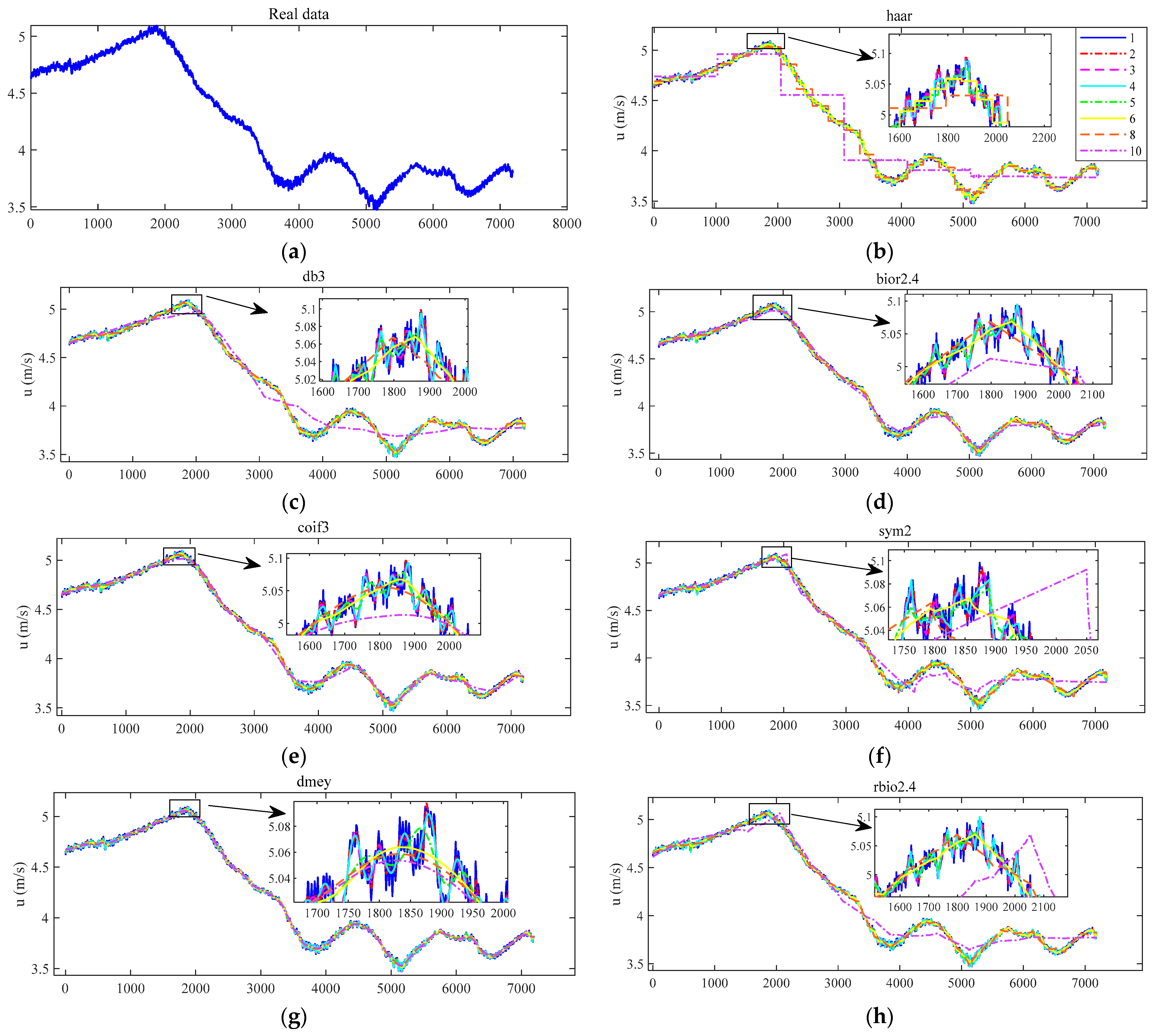
As an example of the 20°/20° Horizontal ZigZag test (HZZ), surge velocity is decomposed using 1, 2, 3, 4, 5, 6, 8, and 10 layers for different basis functions, as shown in Figure 2. This leads to the optimal wavelet basis functions and number of layers required in this paper.

Figure 2.
Different decomposition curves with varies basis function of suge velocity. (a) Noise Data Curve; (b) curves of haar; (c) curves of db3; (d) curves of bior2.4; (e) curves of coif3; (f) curves of sym2; (g) curves of dmey; (h) curves of rbio2.4.
The above process shows that different wavelet basis functions will result in different filtering curves. The basis function haar is a rectangular wave, with the increasing number of layers, the filter will gradually lose the characteristics of the original signal, the number of layers is too high and too low will affect the effect of noise reduction, the function is selected to decompose the number of layers of the noise reduction curve for 6. Base function db3 in the signal reconstruction process is relatively smooth, in the signal analysis and reconstruction will produce a certain phase distortion. The function selected decomposition of the number of layers for the noise reduction curve of 8. The base function bior2.4 is a linear wave, with the increase of the number of layers, the curve smoothness gradually decreases. The function is selected to decompose the number of layers of the noise reduction curve for 6. The base function coif3 has better symmetry than the db3 function, and the degree of smoothness is also better, and the function is selected to decompose the noise reduction curve with the number of layers of 8. The base function sym2 can reduce the phase distortion of the signal reconstruction with the increase in the number of decomposition layers, the degree of smoothness decreases, the original signal characteristics are gradually lost, and the function is selected to decompose the number of layers of the noise reduction curve for 5. The base function dmey relative smoothness is better, retaining the original signal characteristics more comprehensively; the function selected decomposition layer number of 10 noise reduction curves. Base function rbio2.4 with the increase in the number of layers, the signal is gradually distorted, and the function selected decomposition of the number of layers for the noise reduction curve of 6. The selected curves are plotted in a graph to compare the noise reduction effect, as shown in Figure 3.

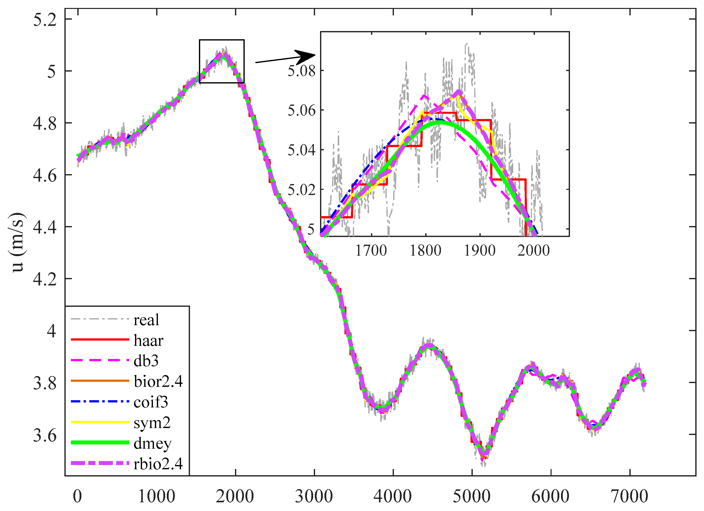
Figure 3.
Noise reduction based on wavelet and comparison for different basis functions.
The obtained noise reduction curves were analyzed for signal-to-noise ratio (SNR), mean square error (MSE), and normalized correlation coefficient (NCC), respectively, and collated into Table 1, and it was found that the base function of dmey was the most effective by comparison, which can also be clearly reflected in Figure 3. Therefore, in this paper, the wavelet denoising method with improved threshold function, dmey basis function, and the number of decomposition layers of 10 layers is used to carry out the noise reduction process for AUV linear velocity. The obtained noise reduction will improve the data accuracy before model training.

Table 1.
Noise reduction error for different basis functions.
3. AUV Identification Model Construction
3.1. AUV Dynamical Mechanism
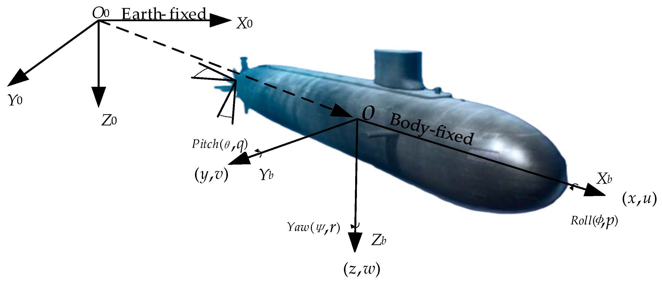
To describe the AUV maneuvering motion [42], two right-handed coordinate systems are used, as shown in Figure 4. For the earth-fixed system , the origin is set as the undisturbed free surface; the axis points to due north, the axis points to due east, and the axis is vertically down. For the body-fixed system , the origin is located in the middle of the ship; the axis points to the bow, the axis points to the starboard side, and the axis points down. and denote vertical and horizontal rudder, respectively. In the body-fixed coordinate system, the translation motions of the AUV are surge, sway, and heave; and the rotational motions are roll, pitch, and yaw. The 6-DOF hydrodynamic model that is Equation (5) of the underwater vehicle AUV proposed by Fossen is used [43]:
where
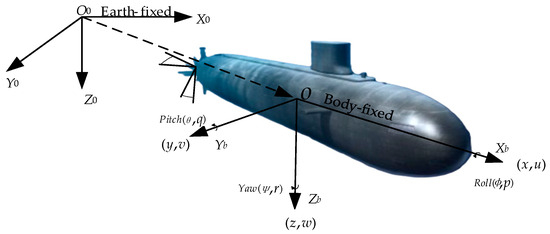
Figure 4.
AUV earth-fixed and body-fixed coordinate systems.
According to Equation (5) it is possible to derive:
where m is the mass of the AUV; are the velocities of the AUV in the x, y, and z directions; are roll, pitch, and yaw angles; are rolling, pitching, and yawing velocity; represents the inertia matrix; is the velocity transformation matrix from the body-fixed system to the earth-fixed system; is the rigid body inertia matrix; and is the additional mass matrix; is the Koch and centrifugal matrix; is the Koch and centrifugal matrix for the mass of the AUV hull; is the Koch and centrifugal matrix for the water surrounding the AUV;
is the damping matrix; is the gravity and buoyancy matrix; and h is the time step. is the combined force of control, resistance, and lift.
3.2. TCN Model
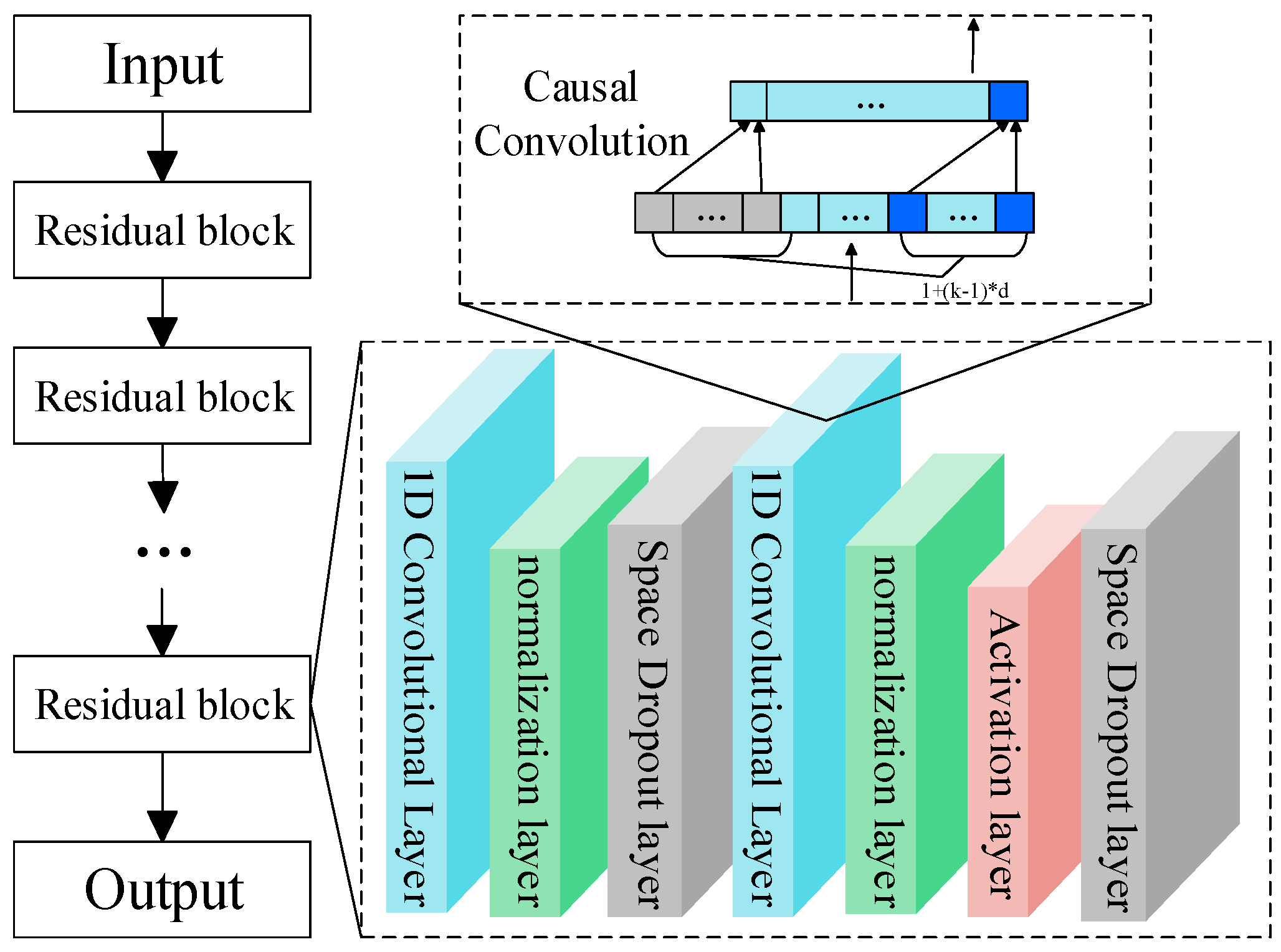
AUV motion data [44] are multidimensional time series, and the motion state at a certain moment is a one-dimensional vector. TCN combines the features of traditional convolutional networks [45] and the ability to adapt to data sequences. TCN is a network structure designed for processing time series data, which can capture the local dependencies of AUV motion states. The TCN consists of residual blocks stacked together, and each residual block contains three parts, temporal causal convolution, dilation convolution, and residual links, and the TCN model is shown in Figure 5. Causal convolution, as a unidirectional structure, is a strictly time-constrained model, which is affected by the AUV motion variables at the previous moment. Expansion convolution is a convolution operation that introduces expansion factors on the basis of causal convolution, which can avoid the problems of gradient vanishing and gradient explosion that exist in the construction of AUV motion models by recurrent neural networks. Residual connections can combine the input information of the residual block with the output information of causal convolution so that the constructed neural network can transmit AUV feature information across layers. The TCN model can extract the deep features of the AUV sequence data, which not only maintains a large sensory field for the data but also reduces the computational volume [46].
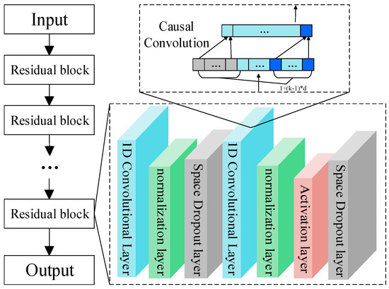
Figure 5.
TCN model structure.
3.3. GRU Model
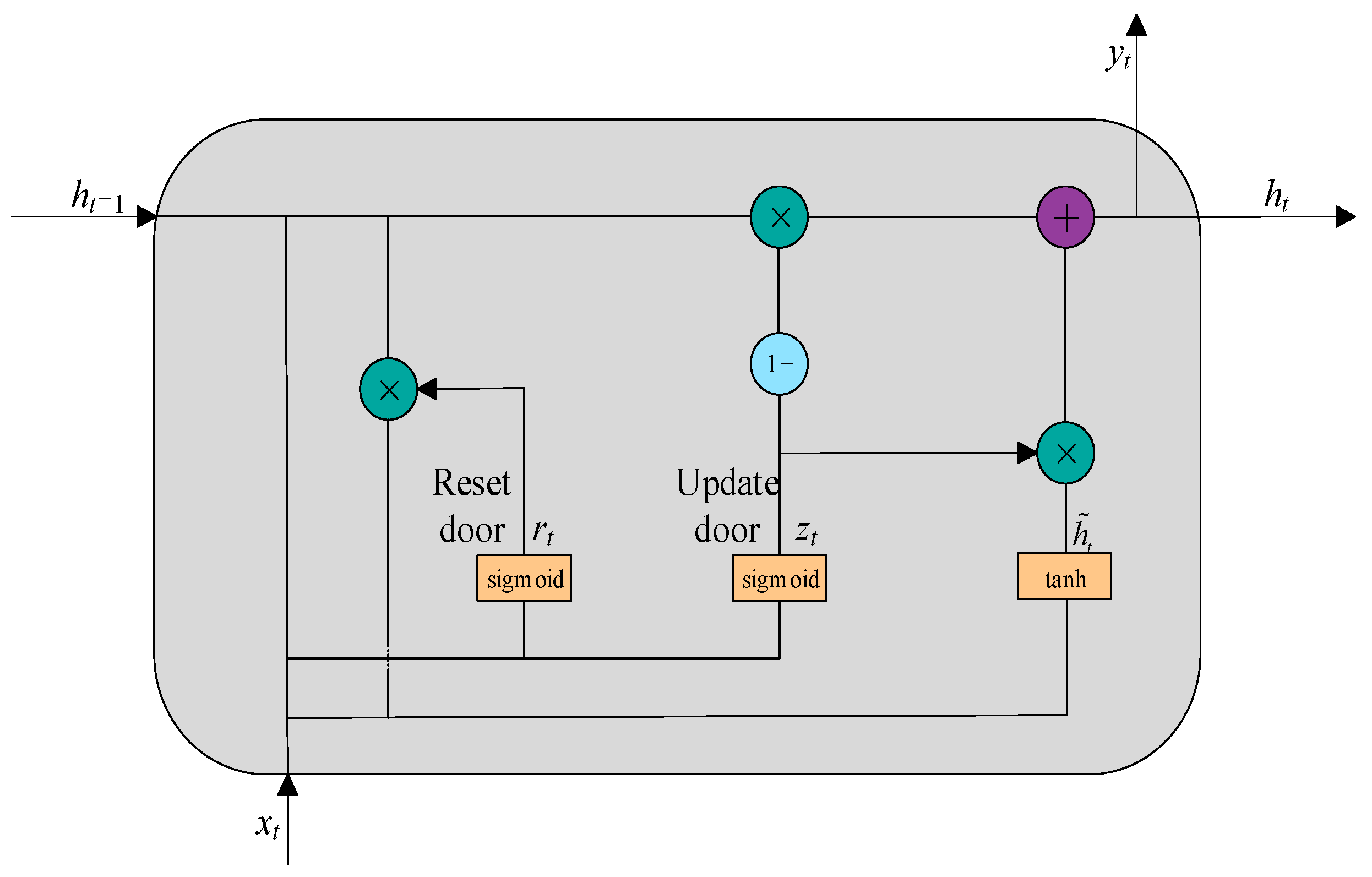
GRU [19] is a neural network developed on the basis of LSTM [47]. The input gate, forget gate, and output gate in LSTM are changed into two gates: update gate and reset gate. It is simpler compared to the LSTM model, while maintaining the same effect as LSTM. The schematic diagram of GRU is shown in Figure 6. The computational equation of the GRU is Equations (10)–(13). BiGRU, as an improved bi-directional recurrent neural network structure, is able to better capture the interdependencies between AUVs.
where is the sigmoid activation function; is the current input value (last activation value); and are the weight matrix and bias vector, respectively; and are the matrix and bias vector of the reset gate, respectively; is the reset gate of the GRU at time t; is the update gate of the GRU at time t; is the weight matrix for the cyclic connection; and denotes the product of Hadamard.
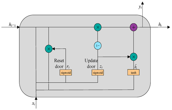
Figure 6.
GRU model structure.
3.4. Self-Attention Model
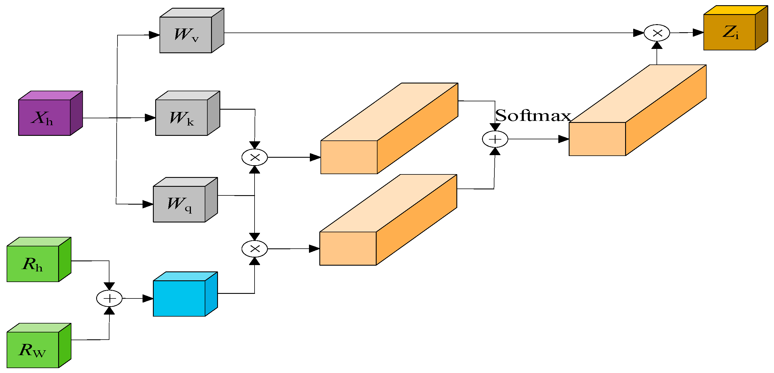
Self-attention [48] (Attention) is a mechanism for sequence modeling and feature extraction, and can be used by dynamically focusing on AUV motion-related feature information. The multihead self-attention mechanism achieves more comprehensive associated features by integrating multiple parallel computed single-head self-attention mechanisms, and in this paper, the single-head attention mechanism is selected for the AUV motion state. The model is shown in Figure 7. The computational equation of the attention mechanism is Equation (14):
where function is the normalized exponential function; is the key vector; is the query vector; is the value vector; is the height matrix; is the width matrix; is the output of the attention mechanism.

Figure 7.
Self-attention model structure.
3.5. DTCN Model
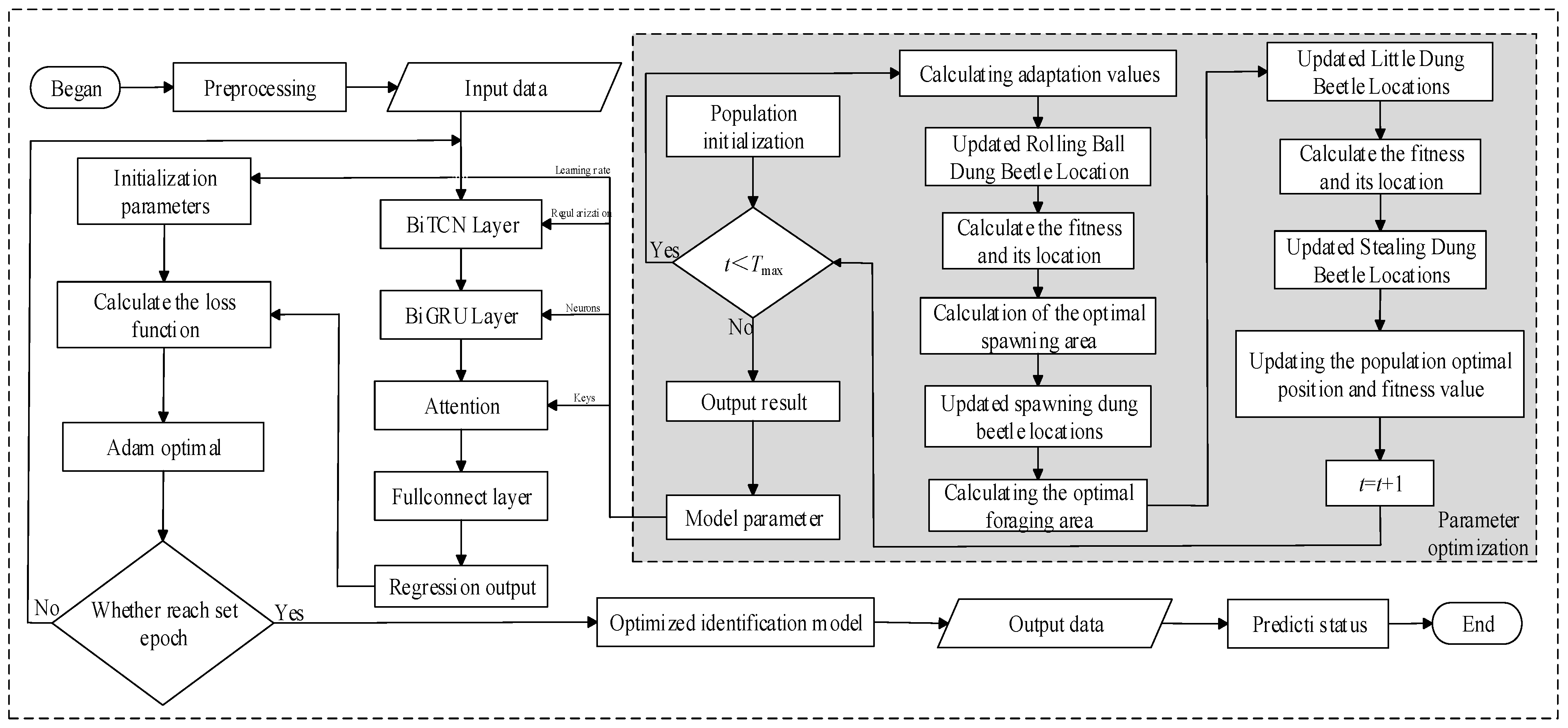
In this paper, the DTCN model is constructed as shown in Figure 8, using the AUV model to obtain the model test data; the raw data is preprocessed to reduce the error of model training. BiTCN, BiGRU, and attention mechanisms are combined to construct the DTCN model, and the model training is completed using the training data. Validation is carried out using ship model data to analyze the forecasting accuracy of the model. Due to the complexity of AUV motion, the construction of the model is different from the methods proposed by other scholars [49], and some important numerical settings are shown in Table 2. The construction method with multiple inputs and single output is used, which is consistent with the nonlinear characteristics and strong coupling characteristics of the AUV. Each time the DTCN outputs a parameter, the parameters identified in this paper need to use a total of six times of DTCN.
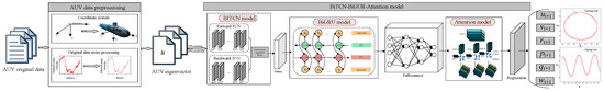
Figure 8.
The proposed DTCN model structure for AUV nonparameter identification.
Table 2.
Parameters of DTCN.
When building a motion model for underwater vehicle maneuvering, training samples need to be constructed to train the model and obtain a nonlinear model [50]. Only the measured motion data at a certain moment is used to predict the motion of the AUV. According to Equation (5), the motion variable is defined as the state vector , the commanded vertical rudder angle is the external input, and the hydrodynamic force and moment are the nonlinear functions of the state vector and the external input. Then, the motion equation can be rewritten as a nonlinear function F, which is a mapping of Equation (8).
Nonparametric identification methods that build nonlinear models by fitting the input and output data of nonlinear systems are the main form of current black box identification. Once the DTCN model of the nonlinear function F is obtained, the maneuvering motion of the ship can be predicted based on the input features. Firstly, the dataset of training samples, including input and output data, is determined. According to Equation (15), the input data contains the state vector and the rudder angle , and the output data are the next moment values of the surge, sway, and heave velocity, and the rolling velocity, pitching velocity, and yawing velocity.
4. Optimization of DTCN Model Parameters
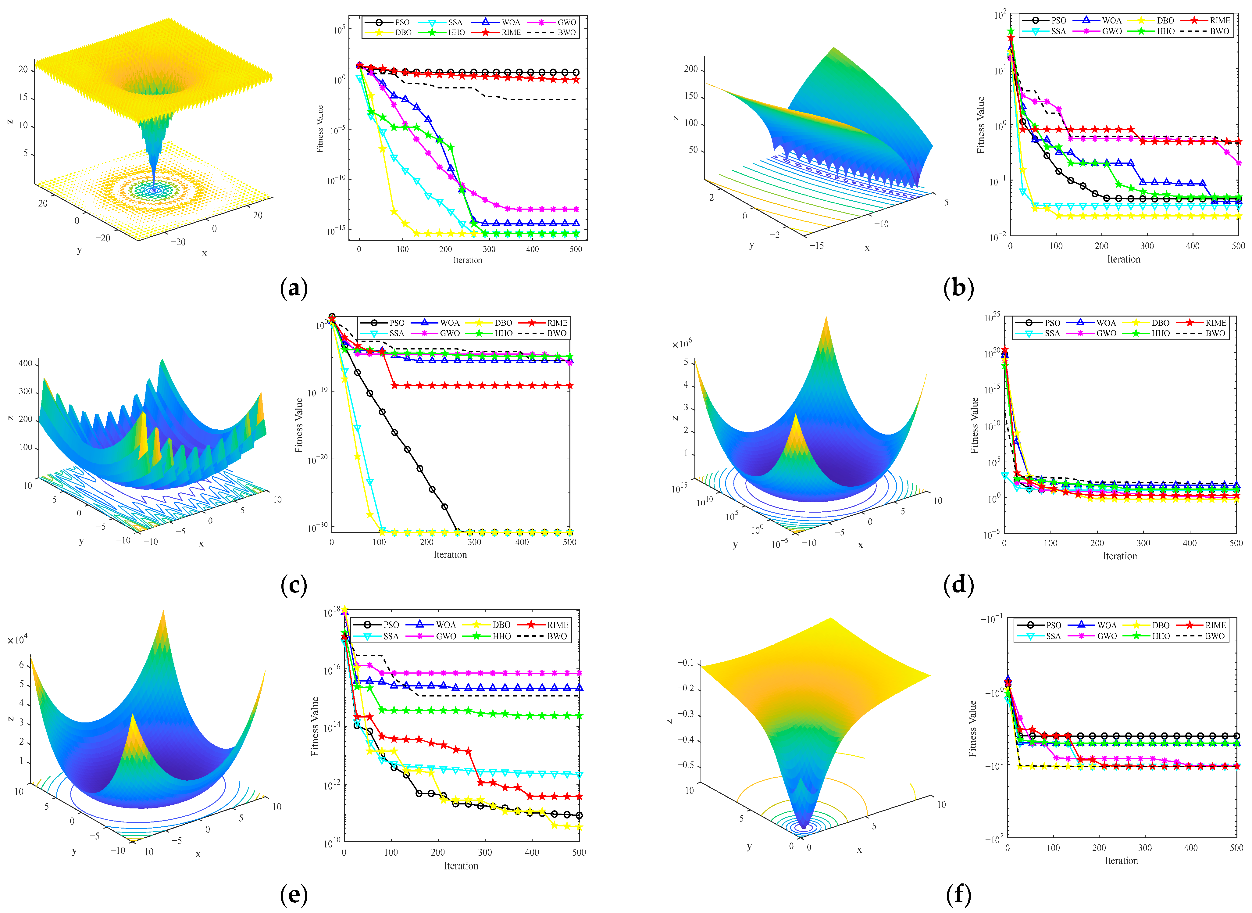
In this paper, the DTCN model is constructed to ensure that the prediction of the AUV motion state is more accurate, and at the same time, to reduce the unnecessary time consumption of prediction as much as possible, this section adopts the optimization algorithm to optimize the parameters of the four hyperparameters in the DTCN. In this paper, the dung beetle optimization algorithm is selected [51]. Through the research of scholars, the DBO algorithm for the optimization of neural networks is faster convergence and better iteration compared to other swarm intelligence optimization algorithms [52,53]. By setting different functions and comparing the POS, Whale Optimization Algorithm (WOA), Rime Optimization Algorithm (RIME), Sparrow Search Algorithm (SSA), GWO, Harris Hawk Optimization Algorithm (HHO), and Beluga Whale Optimization Algorithm (BWO), we can conclude the advantages and disadvantages of the DBO optimization algorithm, and the comparison results are shown in Figure 9.

Figure 9.
Three-dimensional plot of the different functions and convergence curves. (a) F1 function and convergence curves; (b) F2 function and convergence curves; (c) F3 function and convergence curves; (d) F4 function and convergence curves; (e) F5 function and convergence curves; (f) F6 function and convergence curves.
4.1. Dung Beetle Optimization Algorithm
The DBO is a mathematical modeling of the dung beetle’s rolling, foraging, stealing, and reproduction behaviors. The DBO algorithm consists of four steps as rolling, reproducing, foraging, and stealing. The DBO algorithm is more competitive than other algorithms in terms of exploring or exploiting, and it can explore the search space thoroughly by using the information from different time periods in pursuit of a greater search capability to avoid falling into a local optimum.
4.1.1. Rolling Ball Dung Beetle Position Update Model
The Rolling Dung Beetle explores all of space through the act of rolling a dung ball, and its position update can be divided into two modes, with and without obstacles.
- (1)
- When there are no obstacles ahead, the model is Equation (16):where represents the current number of iterations, denotes the position of the dung beetle at the iteration, is a natural coefficient that usually takes the value of −1 or 1, and denotes whether or not there is a deviation from the original direction. denotes the coefficient of deflection, which is expressed as a constant, and are usually set to 0.1 and 0.3 [54], denotes the global worst position, and denotes the simulated change in light intensity.
- (2)
- When there is an obstacle ahead, the model is Equation (17):where denotes the deflection angle and the position of the dung beetle does not change when is 0, , . denotes the offset between the position of the dung beetle at the iteration and the position at the iteration.
4.1.2. Updated Modeling of Spawning Dung Beetle Locations
The spawning dung beetle moves within the safe range to complete its exploration and exploitation within the safe zone, and the spawning location can be represented as Equation (18):
where denotes the current local optimal position, and denote the lower and upper limits of the spawning area, and denote the lower and upper limits of the optimization problem, and denotes the maximum number of iterations. According to Equation (18), the dynamic process of spawning dung beetle can be defined as Equation (19):
where denotes the position information of the spawning dung beetle at iterations, and and denote two independent random vectors.
4.1.3. Updated Modeling of the Location of Small Dung Beetles
Small dung beetles will look for food in the best foraging areas, location updated to Equations (20) and (21).
where denotes the position of the small dung beetle at the iteration, is a normally distributed random number, and a random vector.
4.1.4. Stealing the Dung Beetle Location Update Model
Stealing dung beetles will steal items from other dung beetles. The location updated to Equation (22).
where is denoted as a random variable conforming to a normal distribution and is a constant value.
4.2. Optimization of DTCN Parameters
The parameters of the DTCN model affect both the training duration and prediction performance. The learning rate reflects the model’s ability to capture the spatiotemporal features of AUV data. A rate that is too high can lead to inaccurate predictions, while a rate that is too low can result in prolonged training times and the risk of getting trapped in local optima, leading to overfitting [55]. The regularization coefficient helps prevent overfitting in the neural network model, resulting in smoother AUV predictions. However, if the coefficient is too small, it will be ineffective, and if too large, it can cause underfitting [56]. The number of neurons impacts the model’s ability to capture AUV time series patterns. A low number of neurons may lead to inadequate training, while too many neurons can reduce the model’s generalization ability. The number of keys in the self-attention mechanism influences the weight distribution of AUV features. If the number of keys is too large, it can slow down training and even cause overfitting; if too small, it may fail to capture effective feature vectors, leading to poor predictions. Therefore, optimization algorithms are needed to fine-tune these four hyperparameters.
The four parameters present in the DTCN model used in this paper are learning rate, regularization parameter, number of GRU, and number of attention mechanism keys. The DTCN uses the DBO algorithm for parameter optimization, and the flowchart is shown in Figure 10.
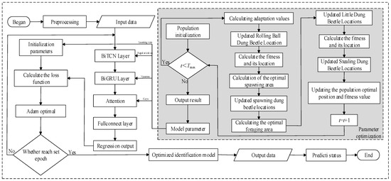
Figure 10.
The proposed flowchart for AUV nonparametric identification based on DBO-DTCN.
5. Study Case and Analysis of AUV Model Identification
5.1. AUV Model Training Setting
In this paper, we use the model test data from the AUV maneuvering, which was carried out at the Netherlands Maritime Research Institute, and the types of model tests include the Turning test, HZZ, and vertical ZigZag test (VZZ). The specific parameters of the AUV are shown in Table 3. The model scale is 18.348, and the Froude number is 0.196. The experimental data used in this paper are all converted to full scale [57], and the full-scale sailing speed is 10 kn. The full-scale rudder rate of turn is 7.11°/s.
Table 3.
Specific parameters of AUV.
The AUV model tests are processed, such as noise reduction and coordinate conversion. The AUV model test data is used to train the DTCN model, and the details of the training dataset are shown in Table 4.
Table 4.
Specific parameters of train test.
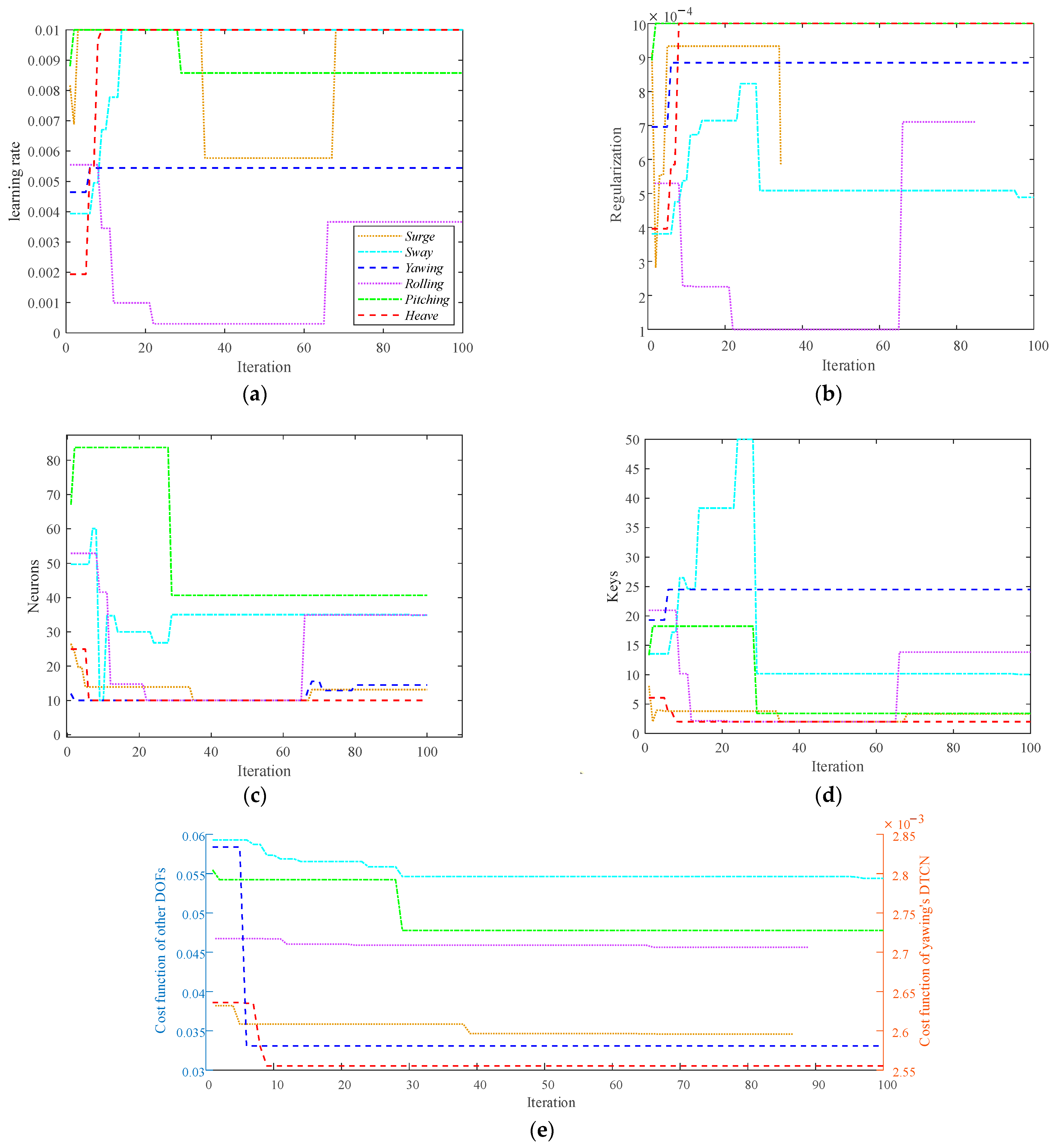
The upper and lower limits of the learning rate, the regularization parameter, the number of neurons, and the number of attention mechanism keys are set to , , and . According to the studies [51,58] and Figure 9, the initial population number is set to 4, the number of iterations is set to 100, and the dimension is set to 4. In this paper, the DBO algorithm is used for the hyperparameter optimization of 6-DOF’s DTCN, and the optimized results are shown in Table 5, and the four-parameter optimization iterations and the cost function convergence of the DTCN are shown in Figure 11. The RMSE of the output in the training data is set as the cost function and can be referenced by Equation (23), for example, the filtered surge velocity and the predicted surge velocity . The RMSE of and is the cost function with iterations for the ship surge motion model.
Table 5.
Optimized hyperparameters of 6-DOF’s DTCN.
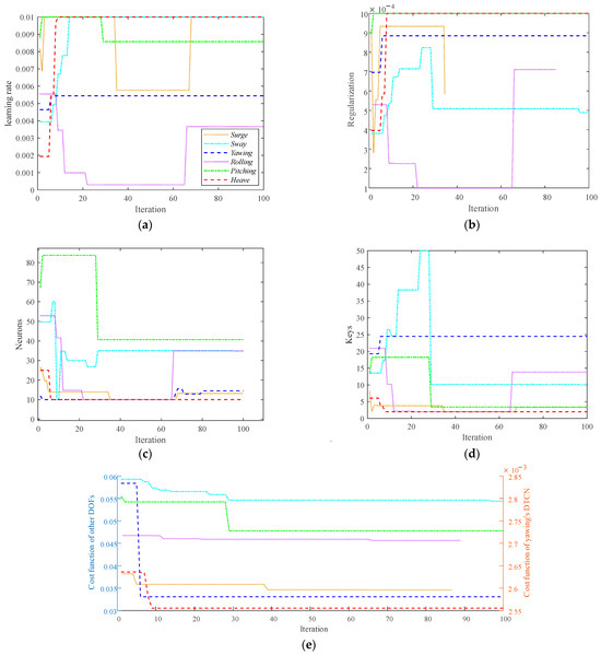
Figure 11.
Cost function convergences of 6-DOF’s DTCN. (a) Learning rate iterative curve; (b) regularization iterative curve; (c) neuron number iterative curve; (d) keys iterative curve; (e) convergent iteration curve of DTCN.
5.2. AUV Model Validation Setting
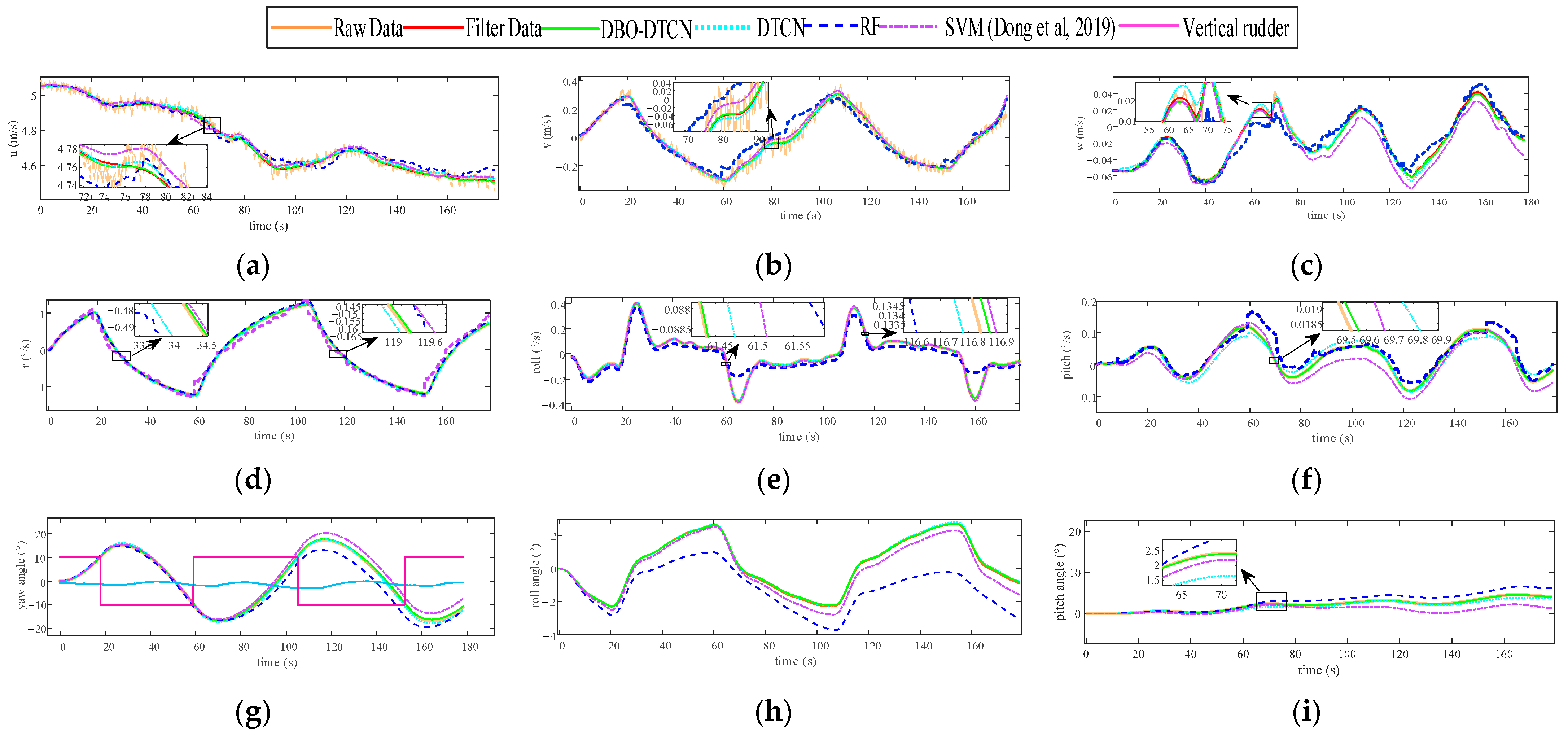
10°/10° HZZ, 10°/10° VZZ, and 20° Turning test are used as the prediction set of the model to verify the generalization ability of the model. In order to reflect the performance of the method in this paper, it is compared with SVM, which method is proposed by scholars [59] and RF. SVM is a widely used method in ship motion modeling [60], and RF is a method with high regression accuracy among integrated machine learning methods [61]. In 10°/10° VZZ, we compare with other different methods. Hydrodynamic models (HDM) [34] and CFD [33] are proposed by some scholars. Finally, different methods are compared, respectively, to verify the accuracy of the optimized DTCN model in this paper.
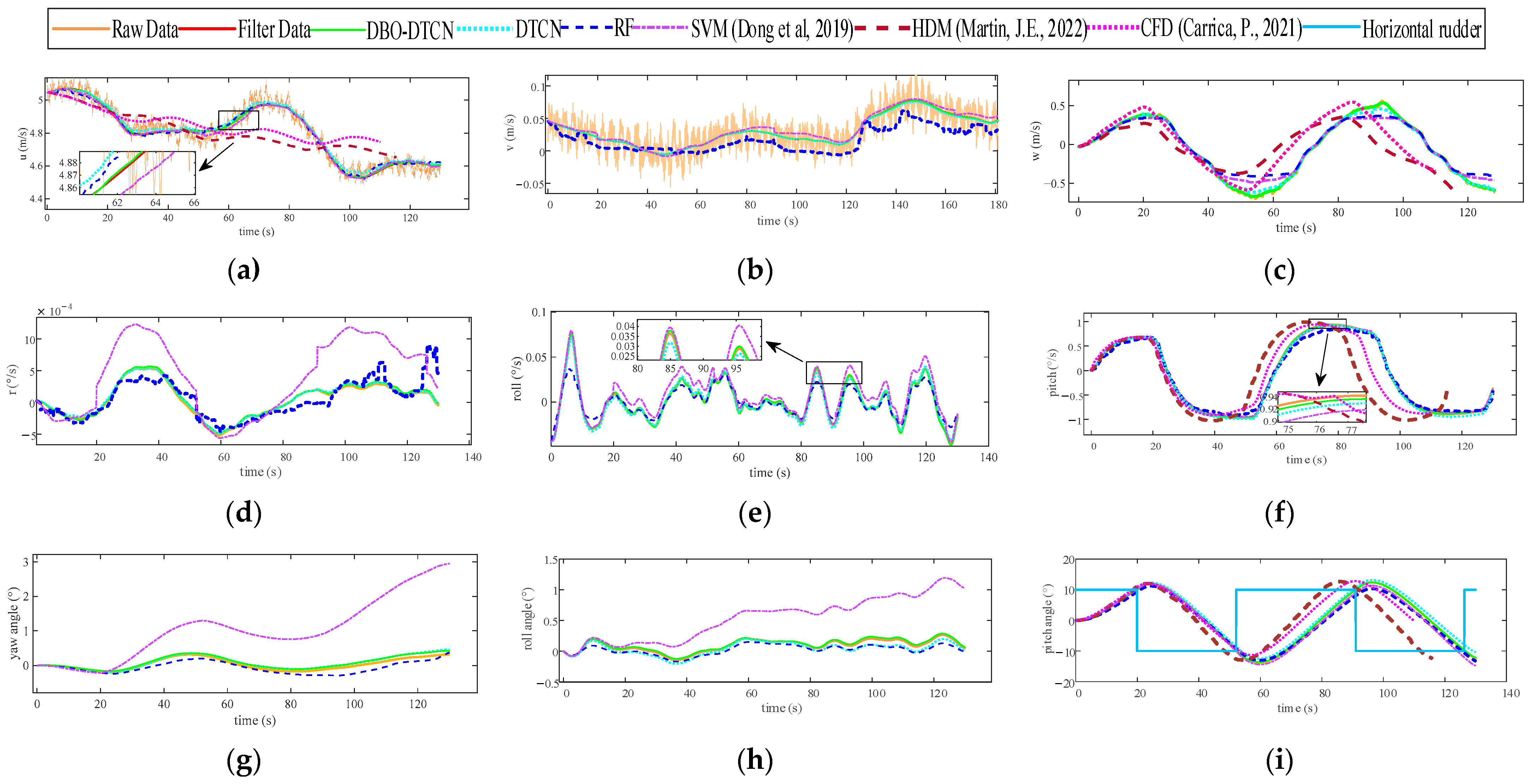
Figure 12 shows the results of 6-DOF motion state prediction for the 10°/10° HZZ. Figure 12a–c are the results of linear velocity prediction for the 10°/10° HZZ, Figure 12d–f are the results of angular velocity prediction for the 10°/10° HZZ, and Figure 12g–i are the results of three attitude angle prediction for the 10°/10° HZZ.
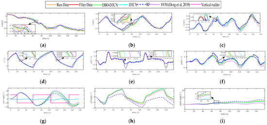
Figure 12.
Validation example of AUV for 10°/10° HZZ; (a) surge velocity; (b) sway velocity; (c) heave velocity; (d) yawing velocity; (e) roll velocity; (f) pitch velocity; (g) yaw angle; (h) roll angle; and (i) pitch angle [59].
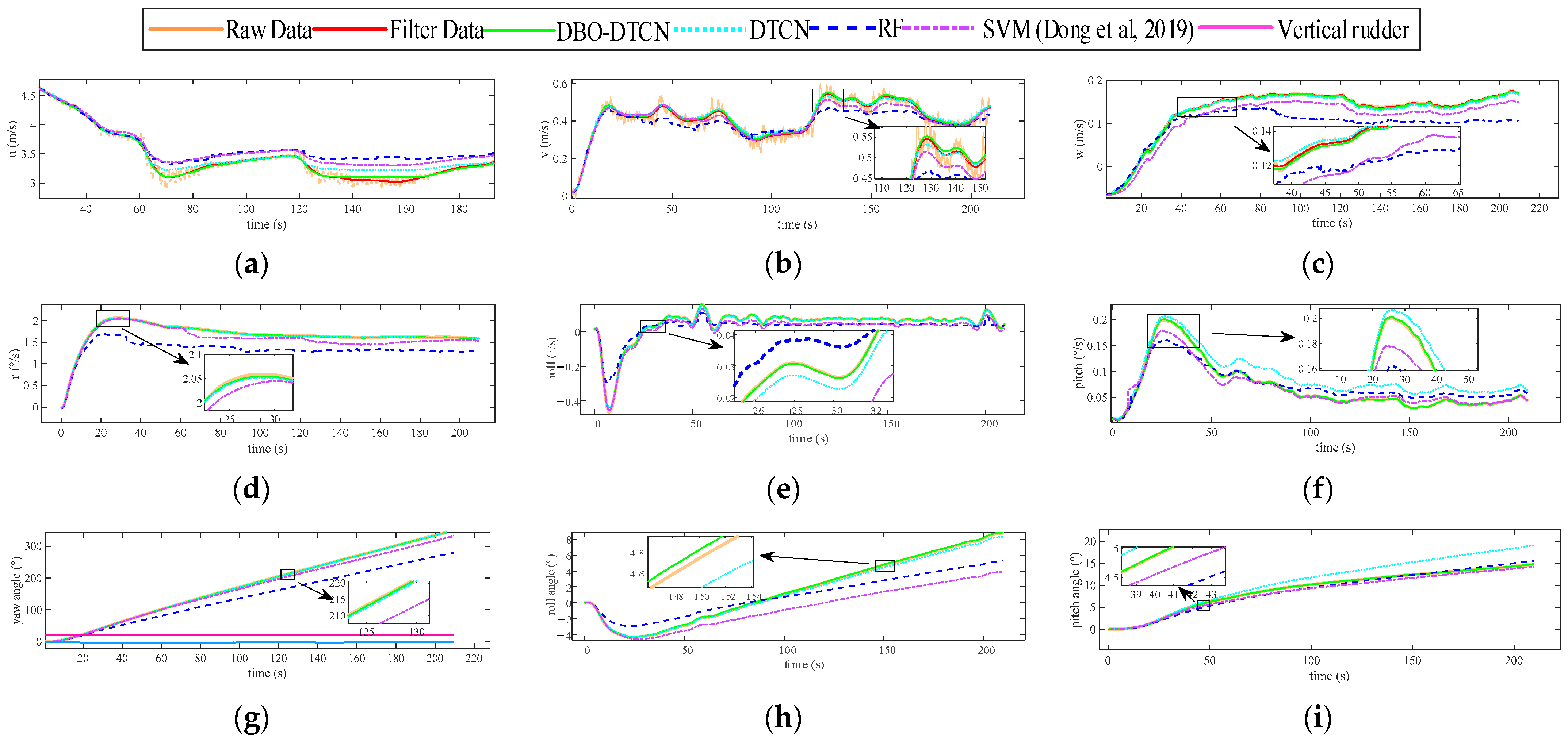
Figure 13 shows the results of 6-DOF motion state prediction for the 10°/10° VZZ. Figure 13a–c are the results of linear velocity prediction for the 10°/10° VZZ, Figure 13d–f are the results of angular velocity prediction for the 10°/10° VZZ, and Figure 13g–i are the results of three attitude angle predictions for the 10°/10° VZZ.
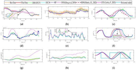
Figure 13.
Validation example of AUV for 10°/10° VZZ. (a) surge velocity; (b) sway velocity; (c) heave velocity; (d) yawing velocity; (e) roll velocity; (f) pitch velocity; (g) yaw angle; (h) roll angle; and (i) pitch angle [33,34,59].
Figure 14 shows the results of 6-DOF motion state prediction for the 20° Turning test. Figure 14a–c are the results of linear velocity predictions for the 20° Turning test, Figure 14d–f are the 20° results of angular velocity predictions for the 20° Turning test, and Figure 14g–i are the results of three attitude angle predictions for the 20° Turning test.
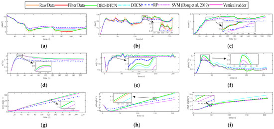
Figure 14.
Validation example of AUV for 20° Turning test. (a) Surge velocity; (b) sway velocity; (c) heave velocity; (d) yawing angular velocity; (e) roll velocity; (f) pitch velocity; (g) yaw angle; (h) roll angle; and (i) pitch angle [59].
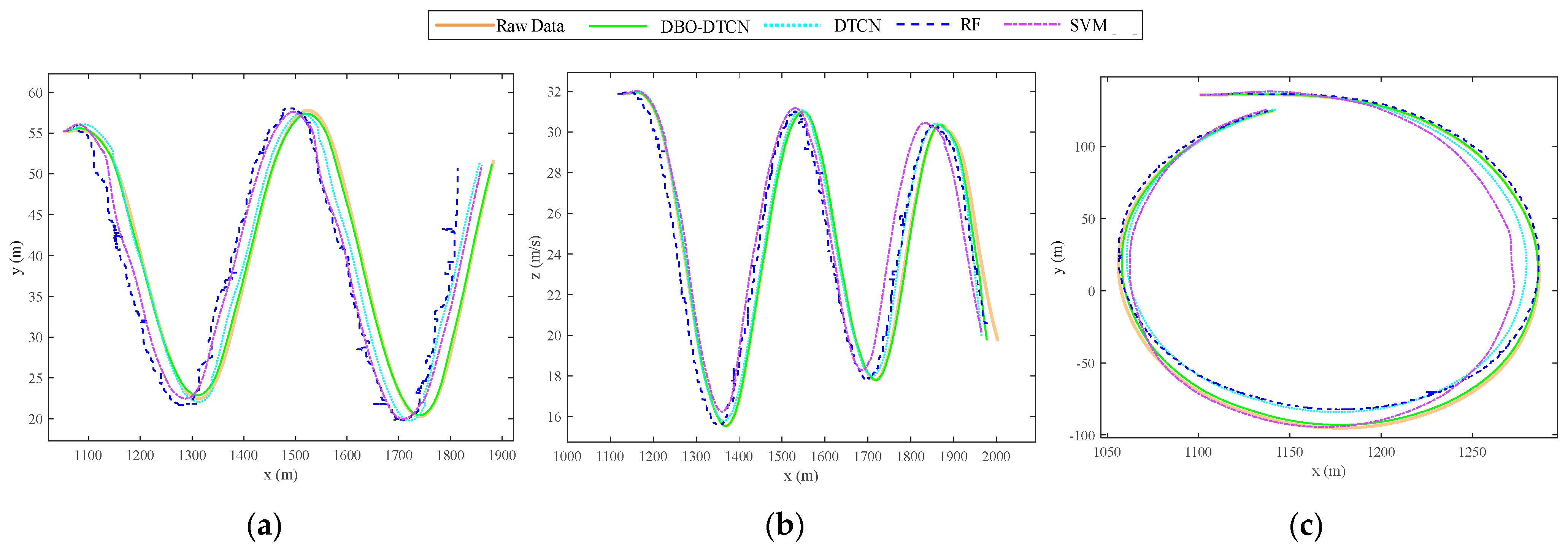
Figure 15 shows the trajectory of the 10°/10° HZZ, the 10°/10° HZZ, and the 20° Turning test.
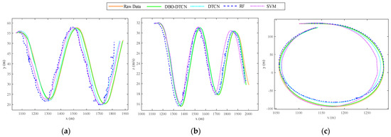
Figure 15.
Validation datasets for AUV DBO-DTCN trajectories. (a) The 10°/10° HZZ; (b) the 10°/10° VZZ; (c) the 20° Turning test [59].
5.3. Error Judgment Index
This section compares the forecast data with the maneuvering basin ship model data using RMSE, SMAPE, and R2 and verifies the accuracy of the model proposed in this paper, the equations for RMSE, SMAPE, and R2 are Equations (22)–(24).
where are the real, mean, and estimated values, respectively. The values of SMAPE range from 0% to 200%. The lower the RMSE and SMAPE, the higher the prediction accuracy. The higher the value of the SMAPE, the better R2 is, the better the prediction performance, which usually takes the value of 0~1.
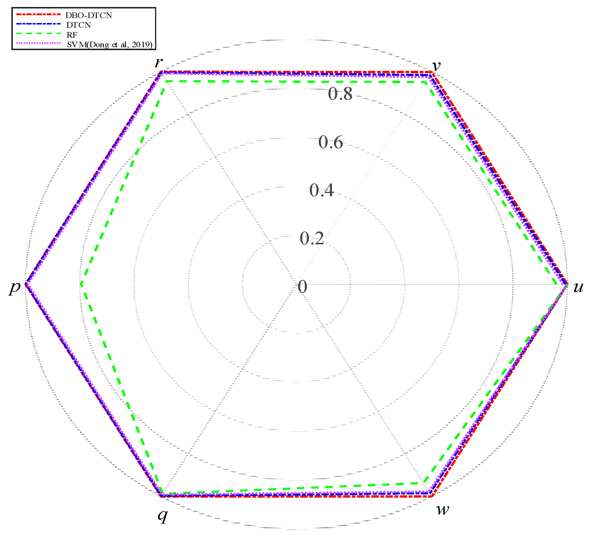
As shown in Figure 16 and Figure 17, the predicted set of data is plotted using radar plots and stacked histograms to verify the prediction accuracy of the DBO-DTCN model. Figure 16 reveals that the data predicted by the DBO-DTCN model has the highest similarity to the original data and the lowest similarity to the RF, especially the lowest similarity of the rolling velocity. Figure 17 shows the highest accuracy of predicted surge velocity in the AUV 6-DOF motion state and the larger prediction error of rolling velocity. The higher frequency of rolling velocity changes and more inflection points cause higher errors in SVM and RF prediction data.
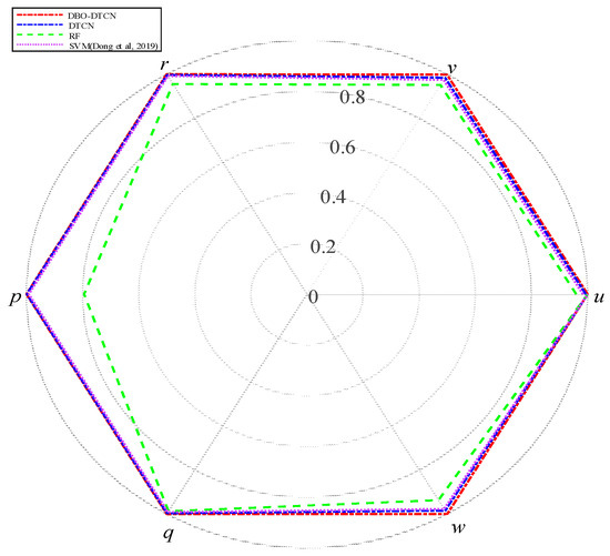
Figure 16.
Radar error of R2 [59].
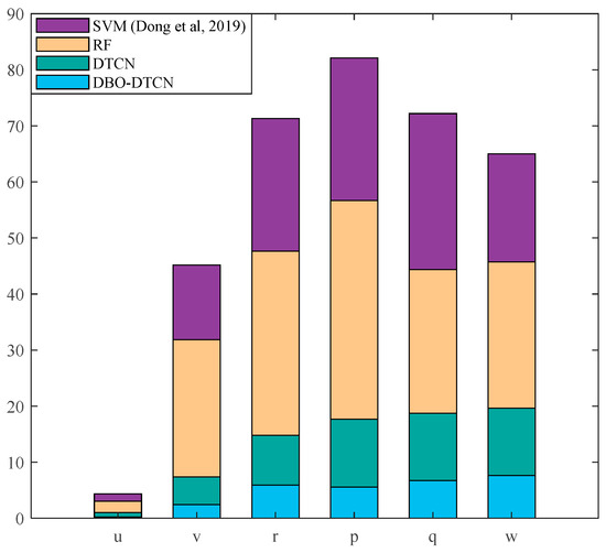
Figure 17.
Stacked bar chart of SMAPE [59].
As shown in Figure 18 and Figure 19, surge velocity and rolling velocity were analyzed using violin statistics [62] and time series error, respectively. The different method of violin shape for the two ZigZag tests in Figure 18 indicates that the HZZ maneuvering capability is different from the VZZ maneuvering capability. RF and SVM have lower errors in the VZZ. The optimized DTCN model error is closer to 0, which is more suitable for the prediction of different types of model tests. Figure 19 shows that the error of DBO-DTCN is affected by the rudder angle, and the model’s rolling velocity prediction produces an error whenever the rudder angle is used. The rolling velocity errors for the HZZ in Figure 19a,b are overall higher than those for the VZZ, and the SVM model for the VZZ predicts more peaks and higher errors. The RF model prediction in Figure 19c shows that the higher peaks lead to larger forecast errors, while the SVM prediction errors gradually stabilize over time. In terms of prediction accuracy, the DBO-DTCN model outperforms the DTCN model, and the DTCN model outperforms the SVM model, which in turn outperforms the RF model. The RMSE, R2, and SMAPE error judgment indices are shown in Table 6.

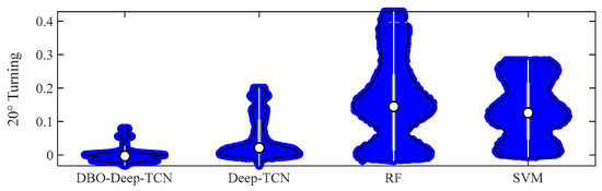
Figure 18.
Violin diagram of surge velocity.
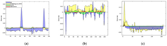
Figure 19.
Errors of predicted roll velocity. (a) 10°/10° HZZ; (b) 10°/10° VZZ; (c) 20° Turning test [59].
Table 6.
Data error and comparison of different methods.
In the DBO-DTCN model, the TCN extracts the feature vectors of the underwater vehicle motion, and the self-attention mechanism applies the weights of different channels to these feature vectors to optimize the temporal representation of the feature vectors. In particular, in conducting the AUV model test, the changes in rudder angle cause significant changes in acceleration, and the optimized DTCN model is able to accurately capture and analyze the dynamic process of these changes and extract the key feature vectors. Since the DBO-DTCN algorithm is able to find the optimal parameter values for the AUV motion state variables, and the DTCN is able to fully capture the nonlinear characteristics of the AUV and addresses the strong coupling problem in modeling.
5.4. Discussion
In this section, we have made HZZ, VZZ, and the Turning test to validate the feasibility of the proposed DBO-DTCN method. In the HZZ test as shown in Figure 12, during the 178 s, the vertical rudder appears four times to reverse the rudder angle, and the yaw velocity, sway velocity, and roll velocity appear as four extreme values at the rudder angle response time point, indicating that the yaw velocity, sway velocity, and roll velocity are strongly coupled, and all of them change with the vertical rudder in the form of a Zigzag shape. The HZZ has less effect on the heave velocity, resulting in a small range of change in heave velocity with a maximum change of 0.02 m/s. During the 0~90 s time period, the surge velocity changes 0.6 m/s. from 5.05 m/s. and the decrease in surge velocity is smaller than that of the Turning test.
In the VZZ, as shown in Figure 13, the horizontal rudder appeared three times to counterpressure the rudder angle; the heave velocity and the pitch velocity both appeared to have three extreme values, indicating that the heave velocity and the pitch velocity are more coupled. This is different from the HZZ, in which the yaw velocity, the sway velocity, and the roll velocity are more strongly coupled.
Via the validation of VZZ, it can be clearly concluded that the model proposed in this paper is more accurate and the error of the HDM method is larger than the others. The HDM and CFD show the worst ability in the surge velocity perdition. In the raw data of the AUV test, the first overshoot angle (OSA) is 2, and the second OSA is 3.72. The performance errors of different models for the OSAs are shown in Table 7. The DBO-DTCN model is the most accurate in OSA predictions.
Table 7.
OSA prediction and error of different methods.
The Turning test shows that the surge velocity decreases 2 m/s in 70 s, deviating from the initial sureg velocity of approximately 38.5%, and therefore, the Turning test are characterized by significant nonlinearity due to the 20° rudder angle. The hydrodynamic force is nonlinear [63]. In other words, is not an exact linear function of the state vector of AUV motion. Therefore, the DBO-DTCN models the nonlinear AUV motion and has certain feasibility.
6. AUV Path Planning and Tracking
6.1. AUV Path Planning
Currently, one of the greatest challenges for AUV is fronting high-quality and reliable paths in complex waters in order to improve the efficiency of AUV SAR. The AUV path planning is mainly based on electronic chart display and information system (ECDIS) [64], elevation maps, ocean environmental data, etc. In this paper, the AUV path planning is mainly based on ECDIS. The SAR area is selected as Ningbo Zhoushan waters, as shown in Figure 20a. Due to the small additional currents near the shore, the influence of the tidal current on the environment is set as constant. ECDIS is widely applied and contains the necessary safety information, such as water depth, obstacles, navigational aids, etc. The first step is to extract the water depth shoreline data through the electronic chart. In this paper, three types of data, namely, land shoreline, isobath, and traffic separation system, are parsed and extracted from the chart data in S-57 format in Figure 20a. Then, a geospatial model of underwater navigation is established, as shown in Figure 20b. It is convenient for AUV to have awareness of the ocean environment. The created environment is shown in Figure 20c,d. In this paper, we compare the algorithm, the algorithm, and the , to plan the best path and suitable waypoints [65].
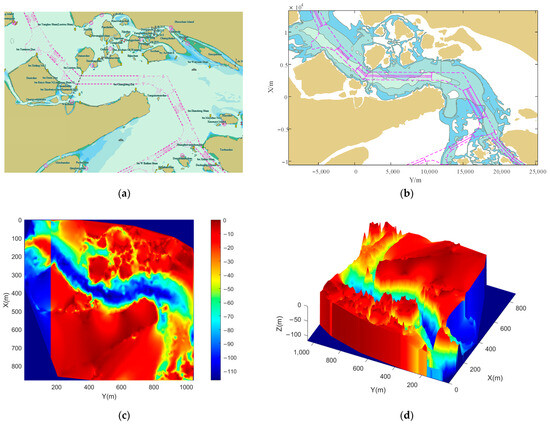
Figure 20.
Marine environmental model based on 3D ECDIS data. (a) ECDIS of Ningbo; (b) vector data based on parsing and extracting ECDIS data; (c) two-dimensional chart of the marine environment; (d) three-dimensional chart of the marine environment.
6.1.1. 3D-A* Algorithm
The traditional algorithm belongs to the heuristic search algorithm [66], which is widely used for static path planning in two-dimensional environments. The traditional two-dimensional algorithm is extended to realize real-time planning of paths in the three-dimensional space. The original two-dimensional algorithm’s cost function of the expands as the Equations (26) and (27).
where are the coordinates of the -th waypoint of the target point under the 3D coordinate system, are the coordinates of its starting point s, and are the coordinates of the target point g. The is the heuristic information intensity function, is the cost function from the starting point to the current position, and is the predicted cost function from the current waypoint to the target point.
6.1.2. Three-Dimensional-Theta* Algorithm
algorithm [67] uses heuristics to find the shortest path. However, does not always compute paths from the current waypoint to its neighboring waypoints. The algorithm allows smooth connections of paths with indirect or nonindirect diagonal shifts of the underlying grid. The arbitrariness of the turning angles can be achieved, and ultimately shorter paths can be found.
6.1.3. Three-Dimensional-lazy-Theta* Algorithm
The algorithm [68] is a variant of the algorithm, and its main improvement lies in the delayed computation of LOS. assumes that LOS exists at the next waypoint after the current waypoint enters close, and performs LOS checking at the end of the path generation, which reduces the LOS checking times and improves the running efficiency of the algorithm. This method accepts suboptimal routes, but only when they have straight paths until final confirmation. If the check fails, the algorithm will fall back and select the next best alternative, eventually finding a feasible path.
6.1.4. Path Planning
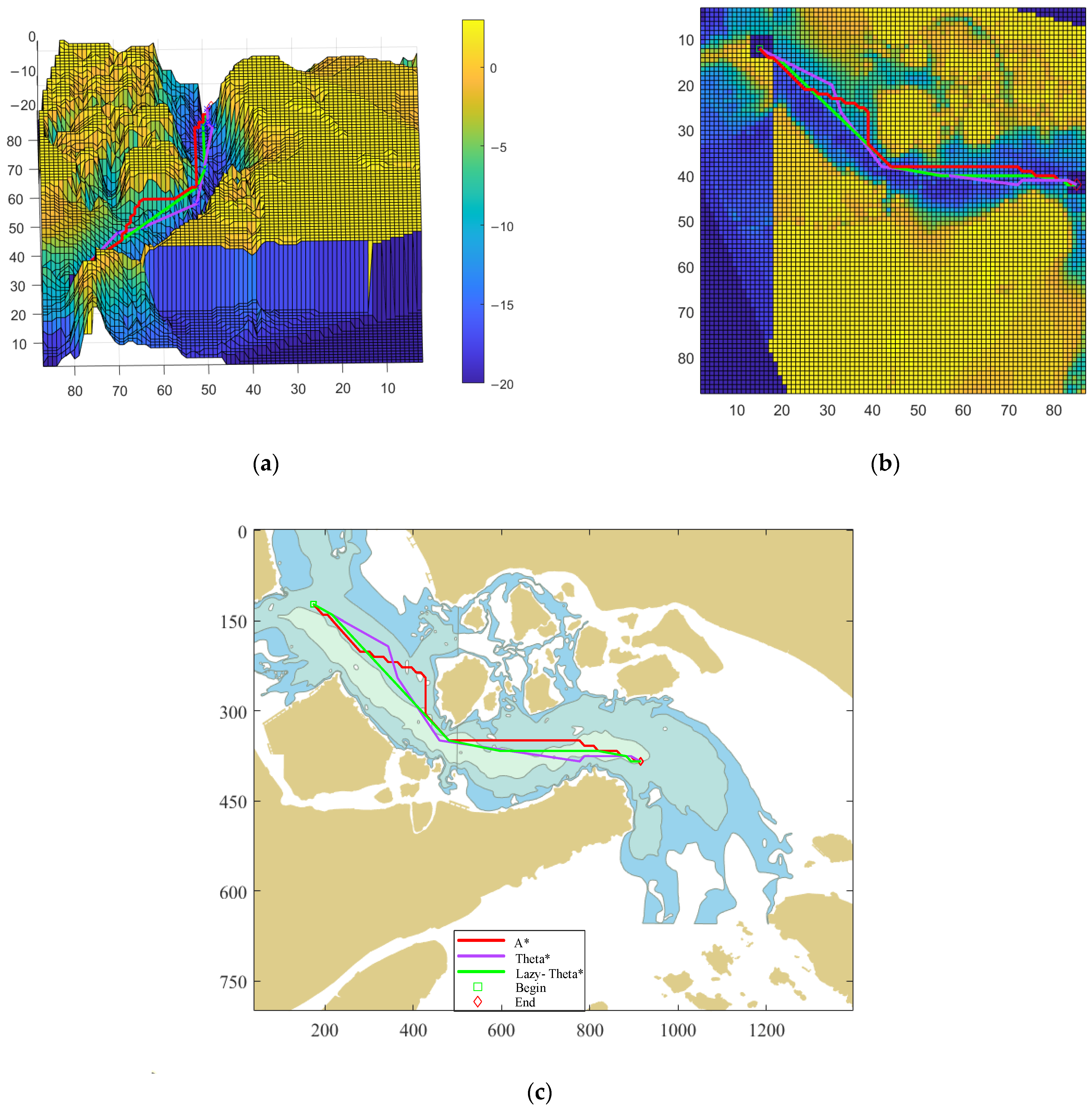
The AUV navigates in the set underwater environment, and the AUV SAR routes are planned according to the three algorithms mentioned above in Section 6, and the scaling of the water area is taken to facilitate the planned routes in order to improve the efficiency of the route setting. The coordinates of the begin waypoint are set to , and the end waypoint is set to , and Figure 21 shows the 3D path planning curves plotted by the three methods. The resulting total distance, average depth, and minimum depth were organized in Table 8.

Figure 21.
Three algorithms path planning diagram. (a) Three-dimensional path planning; (b) two-dimensional path planning; (c) path planning on chart.
Table 8.
Route planning indicators.
Comparing the total distance in Table 8, the route designed by the algorithm in path planning has the shortest distance and saves time, and when the scale of the model is expanded to the modeled sea area, the optimal route can be selected among the time and the length of the path. Therefore, we chose this route as the design planning route so that the trench waters can complete the task of the SAR cruise. Three-dimensional- algorithm designed the path to restore to the water model, the specific parameters of the steering point, as shown in Table 9.
Table 9.
Waypoint list.
6.2. Path Following
In this paper, the above path planning, the path following the planned route is carried out. AUV path following involves several aspects, including navigation control and attitude angle control. In this paper, 3D LOS guidance [69], proportion-integral-differential (PID) bow control, and PID longitudinal tilt control are integrated together to form a complete path-following system.
6.2.1. LOS Algorithm
The navigation principle of the LOS method [70] is based on the variable radius with the minimum circle generated near the path point to generate the desired heading, the LOS angle, and the LOS principle is shown in Figure 22. The effect of the following is realized when the current ship’s heading is consistent with the LOS angle. Set the current following path point as , and the previous path point is , with the AUV location as the center of the circle, and RLOS as the radius of the admittance circle. The point , which is close to , is selected as the LOS point, and it is the angle of the solution of the horizontal plane. In Figure 22: d is the shortest distance from the current position to the following path, and is the forward-looking distance. The reference point position can be derived from Equation (28).
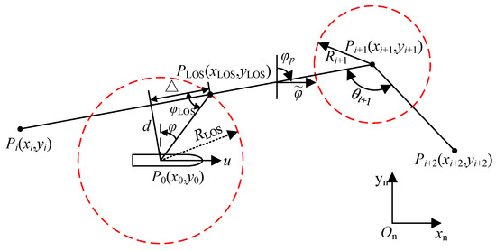
Figure 22.
The LOS principle.
The path tangent direction angle is Equation (29).
The routing process generates errors in Equations (30) and (31).
If stable following of the target path is to be realized, it is necessary to satisfy that is infinitely close to zero when time t is infinite.
6.2.2. Path Following Control System
The following control system used in this paper is PID control, which contains three error feedback mechanisms [71]: proportional control, integral control, and differential control. The PID principle is Equation (32):
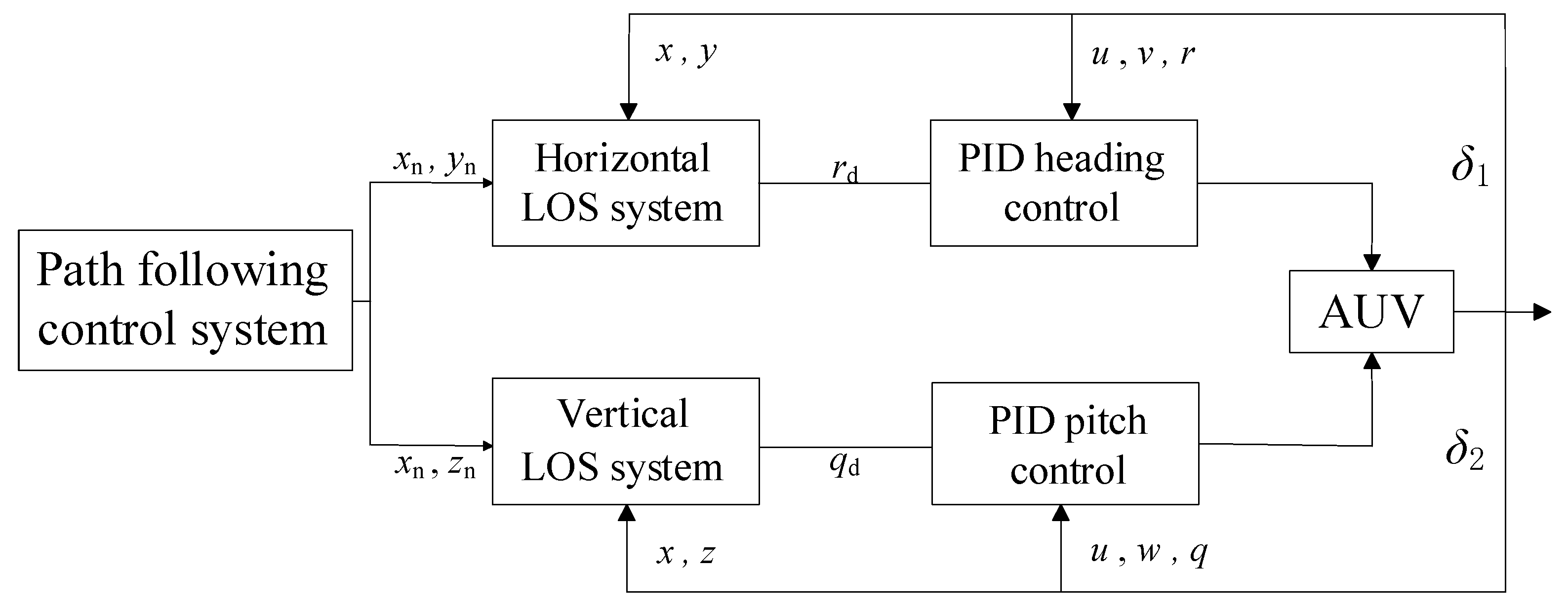
6.2.3. Three-Dimensional Path Following
Due to the coupling between each DOF of the AUV and the weak coupling between the horizontal and vertical motion characteristics, it is possible to design the controller in both the horizontal and vertical planes. The decoupling of the AUV is simplified. The path following the error vector is established, which in turn defines the desired distance from the current position of the AUV to the next moment. When t is infinitely large, and are infinitely close to zero to satisfy the track stabilization tracking. Since there are horizontal and vertical rudders in the AUV, two sets of PID controllers are used in horizontal and depth control. The structure diagram is shown in Figure 23.
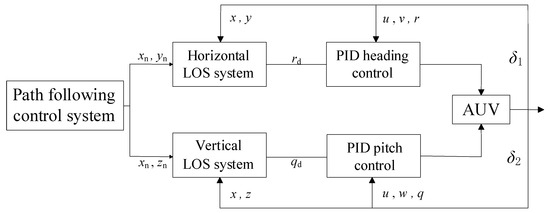
Figure 23.
Path following architecture.
6.2.4. Simulation of AUV Path Following
In order to test the performance of the 3D path following the system, the start coordinates are and the end coordinates are . There are the results of the path following study in Section 6.2.1, resulting in seven waypoints in Table 9. The heading controller scale factor is set to , the pitch controller scale factor is set to , the initial speed is set to is set to m/s, and the ship’s attitude angle is set to , and the propeller rotational speed is 3.86 rps. We set different current speeds to compare results. The current speed is set to kn. The current direction is 135°.
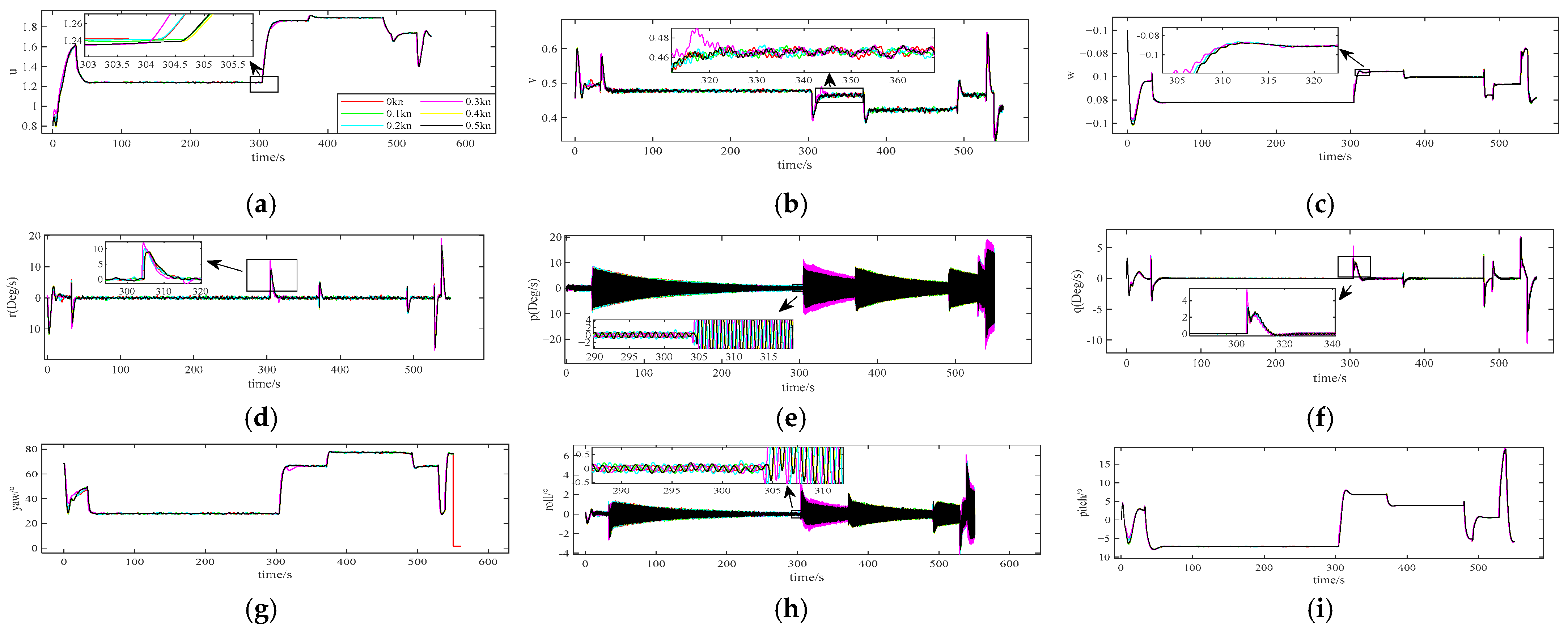
The AUV velocities are shown in Figure 24, including the states of linear velocity, angular velocity, and attitude angle. When the current speed is 0.3 kn, the error is max, especially in the surge and sway velocity in Figure 24a,b.
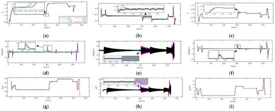
Figure 24.
Path following simulation result with different current speed. (a) Surge velocity; (b) sway velocity; (c) heave velocity; (d) yawing velocity; (e) roll velocity; (f) pitch velocity; (g) yaw angle; (h) roll angle; and (i) pitch angle.
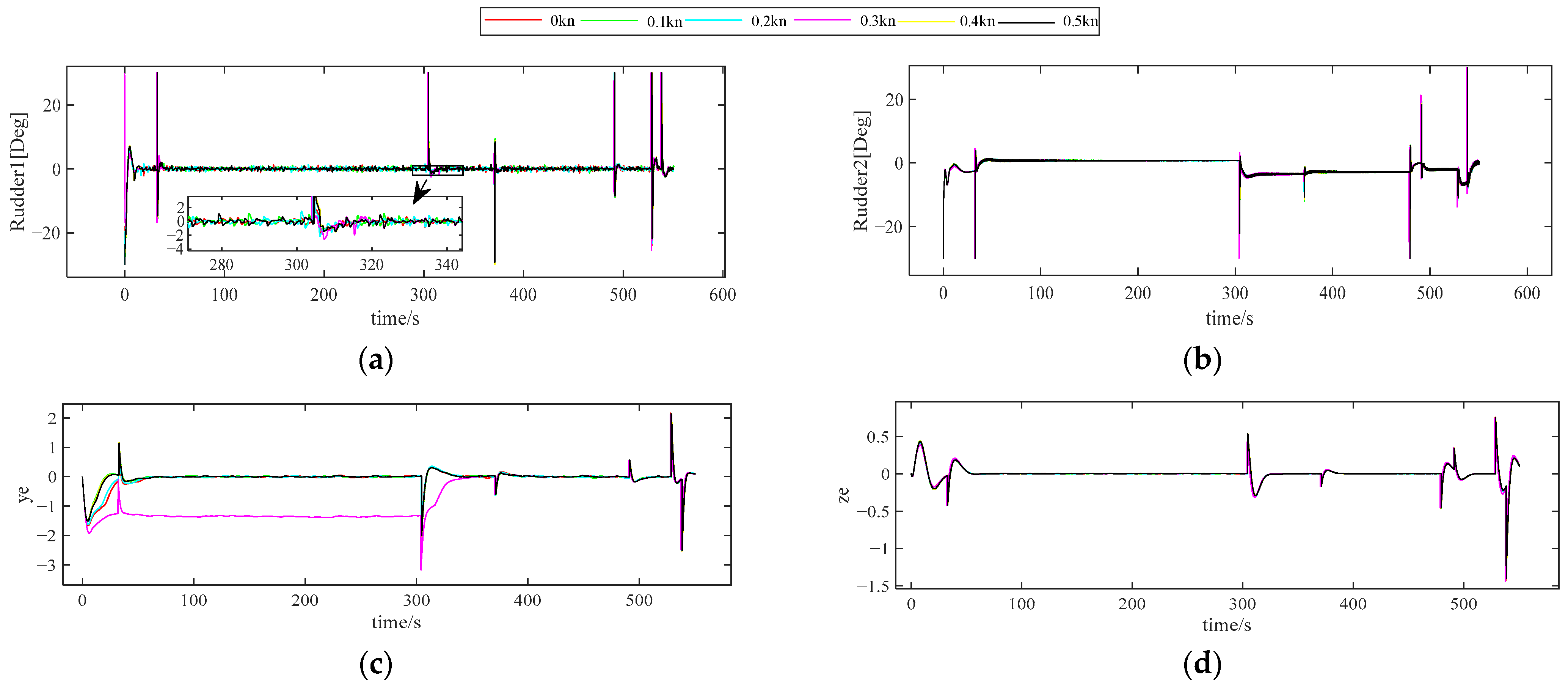
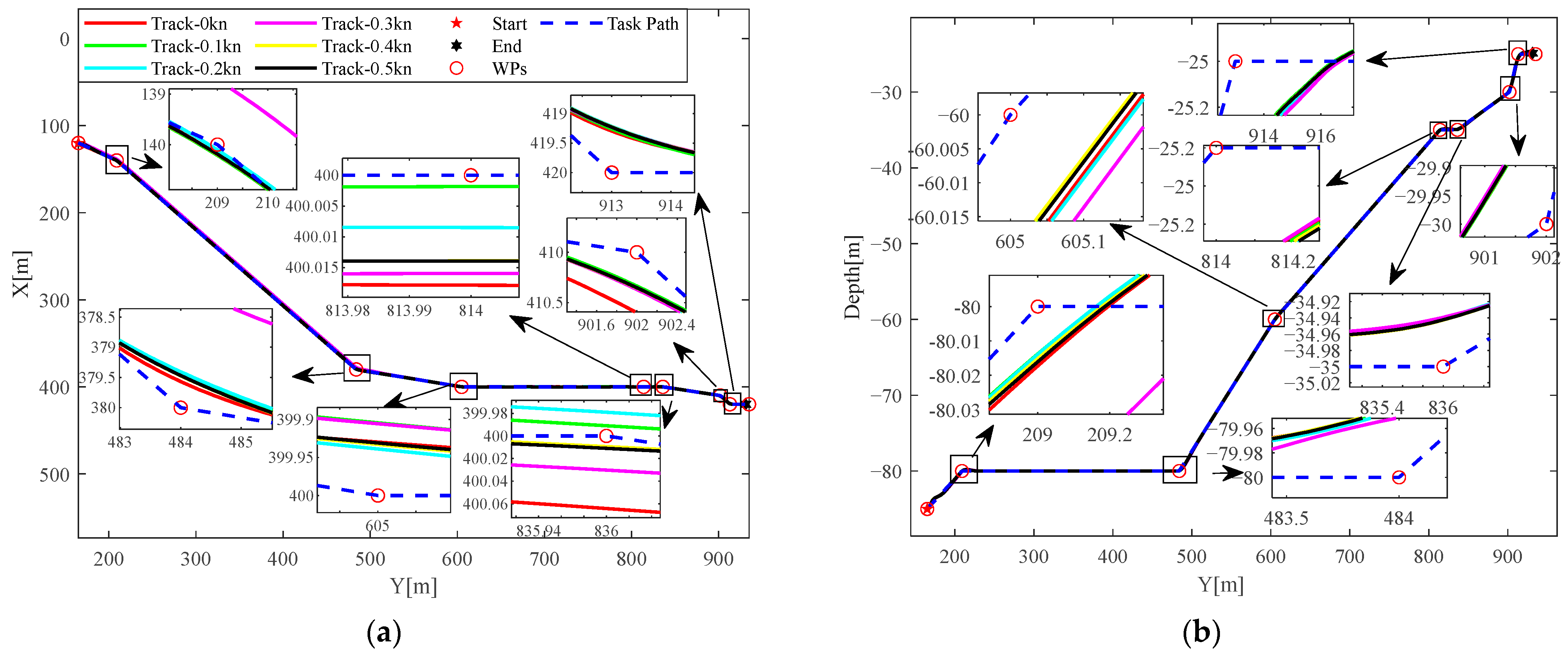
When the rudder is changed, the position errors vary, as shown in Figure 25, and the path following results are shown in Figure 26. From the variation of the two rudder angles, the horizontal rudder (in Figure 25b) makes position errors larger than the vertical rudder (Figure 25a). In Figure 25a,c, the results show that the change of the vertical rudder leads to a 6 times error of , and the maximum error of occurs at approximately 300 s, and the maximum distance of the AUV moving in the y-axis is 935 m as shown in Figure 26a. In Figure 25b,d, the change in the horizontal rudder causes 8 times error in , the maximum error of appears at approximately 520 s, and the maximum depth changes in the AUV is 60 m as shown in Figure 26b. When the effect of current is added in this environment, the gradual change between the individual DOF of the AUV with the current.
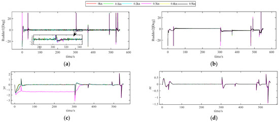
Figure 25.
Rudder outputs and position errors of for AUV path following in SAR. (a) Vertical rudder simulation results; (b) horizontal rudder simulation results; (c) cross-tracking error ey; (d) depth tracking error ez.
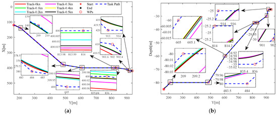
Figure 26.
Track result of AUV path following control at different current speed. (a) Three-dimensional top view; (b) three-dimensional side view.
The actual path and the desired path are shown in Figure 26, and the position errors are shown at the waypoints of Table 9. The 3D path following the control system proposed in this paper is able to accurately track the desired path with good performance. From the path in Figure 26a,b, it can be verified that the proposed AUV model can be used for simulations of marine SAR cruises in trench waters.
7. Conclusions
In this paper, for the 6-DOF AUV, which has characteristics of nonlinearity and strong coupling, a DTCN modeling method based on DBO optimization is proposed, which has been proven effective and feasible after inspecting the AUV ship model data and applied to three-dimensional path planning and following of AUV maneuvering motions, and the results of the study can be applied to the AUV SAR cruising. The following conclusions can be drawn from the simulations.
- (1)
- The improved threshold and basis function in wavelet analysis enhance the filtering effectiveness, making them the crucial parameters for AUV maneuver data filtering. The improved threshold function and dmey basis function are able to reduce the noise in the linear velocity data and improve the accuracy of the prediction model.
- (2)
- The DTCN model captures motion and demonstrates superior prediction performance in nonlinear and coupled scenarios compared to the CFD, HDM, and SVM methods. The BiTCN, BiGRU, and attention are important settings for the DTCN.
- (3)
- The path planning and path following results indicate that the DTCN model is feasible for AUV control to sail through the marine trench. The control errors vary with flow velocity. The DTCN model can be used to simulate the three-dimensional motion of AUV near the seabed.
In this paper, it is shown that the optimized DTCN model provides an effective modeling strategy for underwater vehicle motion. However, in practical applications, the identification modeling process is accelerated by presetting the neural network structure and parameters for AUV motion simulation and by generating data to identify the white box model for AUV route planning and tracking. Although this paper proposes a reliable identification method that does not incorporate environmental factors, they are not included in the proposed model, which may cause errors in the application due to the influence of the environment. Future research will consider AUV motion identification in ocean currents, changes in propeller speed, optimal sampling frequency, online identification model, and optimal energy consumption. In the other aspect, the CFD method can be validated and provide the hydrodynamic data for identification modeling, and the fluid data for flow field recognition.
Author Contributions
B.M. Conceptualization, Methodology, Investigation, Writing—original draft. C.L. Conceptualization, Software, Writing—review and editing, Formal analysis. D.L. Formal analysis, Investigation, Writing—review and editing, Revision. J.Z. Writing—review and editing, Supervision. All authors have read and agreed to the published version of the manuscript.
Funding
DMU navigation college first-class interdisciplinary research project(2023JXA08). Supported by the Fundamental Research Funds for the Central Universities (3132024135), 2023. The Fundamental Research Funds from the Education and Department of Liaoning Province (LJKMZ20220373), 2022.
Institutional Review Board Statement
Not applicable.
Informed Consent Statement
Not applicable.
Data Availability Statement
Data are contained within the article.
Acknowledgments
Heartfelt thanks to Marin in Wageningen from the Netherlands, which offers part of the experimental data. Thanks to Heng Wang for reviewing the paper.
Conflicts of Interest
The authors declare no conflicts of interest.
References
- Bhatt, E.C.; Viquez, O.; Schmidt, H. Under-ice acoustic navigation using real-time model-aided range estimation. J. Acoust. Soc. Am. 2022, 151, 2656–2671. [Google Scholar] [CrossRef] [PubMed]
- Polymenis, I.; Haroutunian, M.; Norman, R.; Trodden, D. Article Virtual Underwater Datasets for Autonomous Inspections. arXiv 2022, arXiv:2209.06013. [Google Scholar]
- Mei, B.; Sun, L.C.; Shi, G.Y.; Liu, X.D. Ship maneuvering prediction using Grey Box framework via adpitive RM-SVM with minor rudder. Pol. Marit. Res. 2019, 26, 115–127. [Google Scholar] [CrossRef]
- Zhu, W.; Wang, S.; Liu, S.; Yang, L.; Zheng, X.; Li, B.; Zhang, L. Dynamic Multi-Period Maritime Accident Susceptibility Assessment Based on AIS Data and Random Forest Model. J. Mar. Sci. Eng. 2023, 11, 1935. [Google Scholar] [CrossRef]
- Bai, W.W.; Zhang, W.J.; Cao, L.; Liu, Q. Adaptive control for multi-agent systems with actuator fault via reinforcement learning and its application on multi-unmanned surface vehicle. Ocean Eng. 2023, 280, 114545. [Google Scholar] [CrossRef]
- Xu, H.; Pires da Silva, P.; Guedes Soares, C. Effect of Sampling Rate in Sea Trial Tests on the Estimation of Hydrodynamic Parameters for a Nonlinear Ship Manoeuvring Model. J. Mar. Sci. Eng. 2024, 12, 407. [Google Scholar] [CrossRef]
- Ramire, W.A.; Leong, Z.Q.; Nguyen, H.; Jayasinghe, S.G. Non-parametric dynamic system identification of ships using multi-output Gaussian Processes. Ocean Eng. 2018, 166, 26–36. [Google Scholar] [CrossRef]
- Xue, Y.F.; Liu, Y.J.; Ji, C.; Xue, G.; Huang, S.T. System identification of ship dynamic model based on Gaussian process regression with input noise. Ocean Eng. 2020, 216, 107862. [Google Scholar] [CrossRef]
- Meng, Y.; Zhang, X.K.; Zhang, X.F. Identification modeling of ship nonlinear motion based on nonlinear innovation. Ocean Eng. 2023, 268, 113471. [Google Scholar] [CrossRef]
- Wang, Y.Y.; Zhang, Y.; Xu, D.J.; Miao, W.Q. Improved whale optimization-based parameter identification algorithm for dynamic deformation of large ships. Ocean Eng. 2022, 245, 110392. [Google Scholar] [CrossRef]
- Wang, Z.H.; Soares, C.G.; Zou, Z.J. Optimal design of excitation signal for identification of nonlinear ship manoeuvring model. Ocean Eng. 2020, 196, 106778. [Google Scholar] [CrossRef]
- Zhang, Z.S.; Zhang, Y.; Wang, J.W.; Wang, H.B. Parameter identification and application of ship maneuvering model based on TO-CSA. Ocean Eng. 2022, 266, 113128. [Google Scholar] [CrossRef]
- Shen, W.H.; Yao, J.X.; Hu, X.J.; Liu, J.L.; Li, S.J. Ship dynamics model identification based on Semblance least square support vector machine. Ocean Eng. 2023, 287, 115908. [Google Scholar] [CrossRef]
- Zhang, X.; Zou, Z. Application of wavelet denoising in the modeling of ship manoeuvring motion. J. Ship Mech. 2011, 15, 616–622. [Google Scholar]
- Silver, D.; Huang, A.; Maddison, C.J.; Guez, A.; Sifre, L.; van den Driessche, G.; Schrittwieser, J.; Antonoglou, I.; Panneershelvam, V.; Lanctot, M.; et al. Mastering the game of Go with deep neural networks and tree search. Cah. Rev. The 2016, 529, 484–489. [Google Scholar] [CrossRef]
- Jiang, Y.; Hou, X.R.; Wang, X.G.; Wang, Z.H.; Yang, Z.L.; Zou, Z.J. Identification modeling and prediction of ship maneuvering motion based on LSTM deep neural network. J. Mar. Sci. Technol. 2022, 27, 125–137. [Google Scholar] [CrossRef]
- Wang, N.; Kong, X.J.; Ren, B.Y.; Hao, L.Z.; Han, B. SeaBil: Self-attention-weighted ultrashort-term deep learning prediction of ship maneuvering motion. Ocean Eng. 2023, 287, 115890. [Google Scholar] [CrossRef]
- Dong, Q.; Wang, N.; Song, J.L.; Hao, L.Z.; Liu, S.M.; Han, B.; Qu, K. Math-data integrated prediction model for ship maneuvering motion. Ocean Eng. 2023, 285, 115255. [Google Scholar] [CrossRef]
- Li, M.W.; Xu, D.Y.; Geng, J.; Hong, W.C. A hybrid approach for forecasting ship motion using CNN-GRU-AM and GCWOA. Appl. Soft Comput. 2022, 114, 108084. [Google Scholar] [CrossRef]
- Li, D.; Du, L. AUV Trajectory Tracking Models and Control Strategies: A Review. J. Mar. Sci. Eng. 2021, 9, 1020. [Google Scholar] [CrossRef]
- Chen, T.H.; Zhang, Z.; Fang, Z.; Jiang, D.; Li, G.L. Imitation learning from imperfect demonstrations for AUV path tracking and obstacle avoidance. Ocean Eng. 2024, 298, 117287. [Google Scholar] [CrossRef]
- Li, L.; Li, Y.P.; Wang, Y.L.; Xu, G.P.; Wang, H.L.; Gao, P.Y.; Feng, X.S. Multi-AUV coverage path planning algorithm using side-scan sonar for maritime search. Ocean Eng. 2024, 300, 117396. [Google Scholar] [CrossRef]
- Miao, J.M.; Wang, Y.Y.; Deng, K.K.; Sun, X.Y.; Liu, W.C.; Guo, Z.Q. PECLOS path-following control of underactuated AUV with multiple disturbances and input constraints. Ocean Eng. 2023, 284, 115236. [Google Scholar] [CrossRef]
- Zhi, L.; Zuo, Y. Collaborative Path Planning of Multiple AUVs Based on Adaptive Multi-Population PSO. J. Mar. Sci. Eng. 2024, 12, 223. [Google Scholar] [CrossRef]
- Yao, P.; Qiu, L.Y.; Qi, J.P.; Yang, R. AUV path planning for coverage search of static target in ocean environment. Ocean Eng. 2021, 241, 110050. [Google Scholar] [CrossRef]
- Zhang, W.; Wang, N.; Wu, W. A hybrid path planning algorithm considering AUV dynamic constraints based on improved A* algorithm and APF algorithm. Ocean Eng. 2023, 285, 115333. [Google Scholar] [CrossRef]
- Sui, F.L.; Tang, X.K.; Dong, Z.H.; Gan, X.J.; Luo, P.; Sun, J. ACO plus PSO plus A*: A bi-layer hybrid algorithm for multi-task path planning of an AUV. Comput. Ind. Eng. 2023, 175, 108905. [Google Scholar] [CrossRef]
- Meng, W.L.; Gong, Y.; Xu, F.; Tao, P.P.; Bo, P.B.; Xin, S.Q. Efficient path planning for AUVs in unmapped marine environments using a hybrid local-global strategy. Ocean Eng. 2023, 288, 116227. [Google Scholar] [CrossRef]
- Hua, C.; Wu, N.; Yuan, H.; Chen, X.; Dong, Y.; Zeng, X. Time-Optimal Path Planning of a Hybrid Autonomous Underwater Vehicle Based on Ocean Current Neural Point Grid. J. Mar. Sci. Eng. 2022, 10, 977. [Google Scholar] [CrossRef]
- Li, X.H.; Yu, S.H. Three-dimensional path planning for AUVs in ocean currents environment based on an improved compression factor particle swarm optimization algorithm. Ocean Eng. 2023, 280, 114610. [Google Scholar] [CrossRef]
- Chen, Y.; Zhang, R.M.; Wang, M.Y.; Gao, J.; Destech Publicat, I. Calculation of Hydrodynamic Parameters Using the Simulation of AUV’s 6DOF Motions. In Proceedings of the International Conference on Automation, Mechanical and Electrical Engineering (AMEE), Phuket, Thailand, 26–27 July 2015; pp. 318–324. [Google Scholar]
- Zhao, Z.Y.; Feng, X.L.; Jiang, C.; Zhang, Y.Z.; Su, W.B.; Hu, Q. Distributed short-term predictive control for AUV clusters in underwater cooperative hunting tasks. Ocean Eng. 2024, 301, 117343. [Google Scholar] [CrossRef]
- Carrica, P.; Kim, Y.; Martin, J. Vertical zigzag maneuver of a generic submarine. Ocean Eng. 2021, 219, 108386. [Google Scholar] [CrossRef]
- Martin, J.E.; Hammond, M.; Rober, N.; Kim, Y.; Cichella, V.; Carrica, P. Reduced order model of a generic submarine for maneuvering near the surface. arXiv 2022, arXiv:2212.09821. [Google Scholar]
- Prestero, T. Development of a six-degree of freedom simulation model for the REMUS autonomous underwater vehicle. In Proceedings of the MTS/IEEE Oceans 2001, An Ocean Odyssey. Conference Proceedings (IEEE Cat. No. 01CH37295), Honolulu, HI, USA, 5–8 November 2001; pp. 450–455. [Google Scholar]
- Ramirez, W.A.; Kocijan, J.; Leong, Z.Q.; Nguyen, H.D.; Jayasinghe, S.G. Dynamic System Identification of Underwater Vehicles Using Multi-Output Gaussian Processes. Int. J. Autom. Comput. 2021, 18, 681–693. [Google Scholar] [CrossRef]
- Chen, Y.; Wang, W.J.; Xu, G.H. System Identification of AUV Hydrodynamic Model Based on Support Vector Machine. In Proceedings of the 7th IEEE International Conference on Underwater System Technology-Theory and Applications (IEEE USYS), Univ Teknologi Malaysia, Kuala Lumpur, Malaysia, 18–20 December 2017. [Google Scholar]
- Sutulo, S.; Soares, C.G. An algorithm for offline identification of ship manoeuvring mathematical models from free-running tests. Ocean Eng. 2014, 79, 10–25. [Google Scholar] [CrossRef]
- Zhang, X.; Li, J.L.; Xing, J.C.; Wang, P.; Fu, D.H. A Kent Chaos Artificial Bee Colony Algorithm Based Wavelet Thresholding Method for Signal Denoising. In Proceedings of the 12th World Congress on Intelligent Control and Automation (WCICA), Guilin, China, 12–15 June 2016; pp. 3129–3134. [Google Scholar]
- Deng, G.H.; Liu, Z.L. A Wavelet Image Denoising Based On The New Threshold Function. In Proceedings of the 11th International Conference on Computational Intelligence and Security (CIS), Shenzhen, China, 19–20 December 2015; pp. 158–161. [Google Scholar]
- Liu, H.; You, Y.Q.; Li, S.J.; He, D.; Sun, J.; Wang, J.W.; Hou, D. Denoising of Laser Self-Mixing Interference by Improved Wavelet Threshold for High Performance of Displacement Reconstruction. Photonics 2023, 10, 943. [Google Scholar] [CrossRef]
- Miller, L.; Brizzolara, S.; Stilwell, D.J. Increase in Stability of an X-Configured AUV through Hydrodynamic Design Iterations with the Definition of a New Stability Index to Include Effect of Gravity. J. Mar. Sci. Eng. 2021, 9, 942. [Google Scholar] [CrossRef]
- Sagatun, S.I.; Fossen, T.I. Lagrangian formulation of underwater vehicles’ dynamics. In Proceedings of the Conference Proceedings, IEEE International Conference on Systems, Man, and Cybernetics, Charlottesville, VA, USA, 13–16 October 1991; pp. 1029–1034. [Google Scholar]
- Zeng, F.; Zhang, X.; Liu, J.; Li, H.; Zhu, Z.; Zhang, S. Magnetic Gradient Tensor Positioning Method Implemented on an Autonomous Underwater Vehicle Platform. J. Mar. Sci. Eng. 2023, 11, 1909. [Google Scholar] [CrossRef]
- Guo, T.; Xie, L. Research on Ship Trajectory Classification Based on a Deep Convolutional Neural Network. J. Mar. Sci. Eng. 2022, 10, 568. [Google Scholar] [CrossRef]
- Zhang, J.J.; Zhang, T.T.; Chen, J.L. Sentiment Analysis of Chinese Reviews Based on BiTCN-Attention Model. Int. J. Found. Comput. Sci. 2022, 33, 755–770. [Google Scholar] [CrossRef]
- Wang, D.; Wan, J.; Shen, Y.; Qin, P.; He, B. Hyperparameter Optimization for the LSTM Method of AUV Model Identification Based on Q-Learning. J. Mar. Sci. Eng. 2022, 10, 1002. [Google Scholar] [CrossRef]
- Chu, H.L.; Li, C.; Wang, H.B.; Wang, J.; Tai, Y.P.; Zhang, Y.L.; Zhou, L.; Yang, F.; Benezeth, Y. MTSA-Net: A multiscale time self-attention network for ship radiated self-noise reduction. Ocean Eng. 2024, 292, 116566. [Google Scholar] [CrossRef]
- Zhang, B.; Wang, S.; Deng, L.W.; Jia, M.Q.; Xu, J.Z. Ship motion attitude prediction model based on IWOA-TCN-Attention. Ocean Eng. 2023, 272, 113911. [Google Scholar] [CrossRef]
- Xu, H.; Guedes Soares, C. Data-Driven Parameter Estimation of Nonlinear Ship Manoeuvring Model in Shallow Water Using Truncated Least Squares Support Vector Machines. J. Mar. Sci. Eng. 2023, 11, 1865. [Google Scholar] [CrossRef]
- Xue, J.K.; Shen, B. Dung beetle optimizer: A new meta-heuristic algorithm for global optimization. J. Supercomput. 2023, 79, 7305–7336. [Google Scholar] [CrossRef]
- Wang, W.T.; Zhang, Q.J.; Guo, S.; Li, Z.X.; Li, Z.G.; Liu, C.J. Hazard evaluation of goaf based on DBO algorithm coupled with BP neural network. Heliyon 2024, 10, e34141. [Google Scholar] [CrossRef] [PubMed]
- Fu, J.; Wu, C.; Wang, J.; Haque, M.M.; Geng, L.; Meng, J. Lithium-ion battery SOH prediction based on VMD-PE and improved DBO optimized temporal convolutional network model. J. Energy Storage 2024, 87, 111392. [Google Scholar] [CrossRef]
- Zhu, F.; Li, G.S.; Tang, H.; Li, Y.B.; Lv, X.M.; Wang, X. Dung beetle optimization algorithm based on quantum computing and multi-strategy fusion for solving engineering problems. Expert. Syst. Appl. 2024, 236, 121219. [Google Scholar] [CrossRef]
- Bai, W.; Ren, J.; Che, Y.; Zhang, T. Locally optimal locally weighted learning black-box identification modeling for tug manoeuvring. In Proceedings of the 2017 4th International Conference on Information, Cybernetics and Computational Social Systems (ICCSS), Dalian, China, 24–26 July 2017; pp. 231–236. [Google Scholar]
- Zhang, Z.; Ren, J. Locally weighted non-parametric modeling of ship maneuvering motion based on sparse Gaussian process. J. Mar. Sci. Eng. 2021, 9, 606. [Google Scholar] [CrossRef]
- Overpelt, B.; Nienhuis, B.; Anderson, B. Free running manoeuvring model tests on a modern generic SSK class submarine (BB2). In Proceedings of the Pacific International Maritime Conference, Seattle, WA, USA, 14–17 June 2015; pp. 1–14. [Google Scholar]
- Shen, Q.; Zhang, D.; Xie, M.; He, Q. Multi-Strategy Enhanced Dung Beetle Optimizer and Its Application in Three-Dimensional UAV Path Planning. Symmetry 2023, 15, 1432. [Google Scholar] [CrossRef]
- Dong, Z.; Yang, X.; Zheng, M.; Song, L.; Mao, Y. Parameter identification of unmanned marine vehicle manoeuvring model based on extended Kalman filter and support vector machine. Int. J. Adv. Robot. Syst. 2019, 16, 1729881418825095. [Google Scholar] [CrossRef]
- Chen, L.J.; Yang, P.Y.; Li, S.W.; Tian, Y.F.; Liu, G.Q.; Hao, G.Z. Grey-box identification modeling of ship maneuvering motion based on LS-SVM. Ocean Eng. 2022, 266, 112957. [Google Scholar] [CrossRef]
- Ji, H.D.; Wang, H.; Chen, Q.; Ma, X.B.; Cai, Y.K. Corrosion behavior prediction for hull steels under dynamic marine environments by jointly utilizing LSTM network and PSO-RF model. Ocean Eng. 2024, 300, 117371. [Google Scholar] [CrossRef]
- Xu, D.X.; Yin, J.C. An enhanced hybrid scheme for ship roll prediction using support vector regression and TVF-EMD. Ocean Eng. 2024, 307, 117951. [Google Scholar] [CrossRef]
- Ramirez, W.A. Gaussian Processes Applied to System Identification, Navigation and Control of Underwater Vehicles. Ph.D. Thesis, University of Tasmania, Lilyfield, Australia, 2019. [Google Scholar]
- Shu, Y.Q.; Zhu, Y.J.; Xu, F.; Gan, L.X.; Lee, P.T.W.; Yin, J.C.; Chen, J.H. Path planning for ships assisted by the icebreaker in ice-covered waters in the Northern Sea Route based on optimal control. Ocean Eng. 2023, 267, 113182. [Google Scholar] [CrossRef]
- Shu, Y.; Xiong, C.; Zhu, Y.; Liu, K.; Liu, R.W.; Xu, F.; Gan, L.; Zhang, L. Reference path for ships in ports and waterways based on optimal control. Ocean. Coast. Manag. 2024, 253, 107168. [Google Scholar] [CrossRef]
- Yin, C.P.; Tan, C.Y.; Wang, C.Q.; Shen, F. An Improved A-Star Path Planning Algorithm Based on Mobile Robots in Medical Testing Laboratories. Sensor 2024, 24, 1784. [Google Scholar] [CrossRef]
- Liu, C.G.; Zhang, K.; He, Z.B.; Lai, L.H.; Chu, X.M. Clustering Theta* based segmented path planning method for vessels in inland. Ocean Eng. 2024, 309, 118249. [Google Scholar] [CrossRef]
- Yue, Y.L.; Li, Y.H.; Zuo, X. Optimization of subsea production control system layout considering hydraulic fluid pressure loss. Ocean Eng. 2023, 288, 116047. [Google Scholar] [CrossRef]
- Ding, X.; Liu, W.Q.; Wan, J.H.; He, B.; Nian, R.; Shen, Y.; Yan, T.H. ELM and LOS Based Path Tracking for Autonomous Underwater Vehicles. In Proceedings of the Conference on OCEANS MTS/IEEE Charleston, Charleston, SC, USA, 22–25 October 2018. [Google Scholar]
- Yuan, C.R.; Shuai, C.G.; Ma, J.G.; Fang, Y.; Jiang, S.J.; Gao, C.Z. Adaptive optimal 3D nonlinear compound line-of-sight trajectory tracking control for over-actuated AUVs in attitude space. Ocean Eng. 2023, 274, 114056. [Google Scholar] [CrossRef]
- Vadapalli, S.; Mahapatra, S. 3D Path Following Control of an Autonomous Underwater Robotic Vehicle Using Backstepping Approach Based Robust State Feedback Optimal Control Law. J. Mar. Sci. Eng. 2023, 11, 277. [Google Scholar] [CrossRef]


Disclaimer/Publisher’s Note: The statements, opinions and data contained in all publications are solely those of the individual author(s) and contributor(s) and not of MDPI and/or the editor(s). MDPI and/or the editor(s) disclaim responsibility for any injury to people or property resulting from any ideas, methods, instructions or products referred to in the content. |
© 2024 by the authors. Licensee MDPI, Basel, Switzerland. This article is an open access article distributed under the terms and conditions of the Creative Commons Attribution (CC BY) license (https://creativecommons.org/licenses/by/4.0/).