Modeling and Investigation of Long-Term Performance of High-Rise Pile Cap Structures Under Scour and Corrosion

Abstract

High-rise pile cap structures, such as sea-crossing bridges, suffer from long-term degradation due to continuous corrosion and scour, which seriously endangers structural safety. However, there is a lack of research on this topic. This study focused on the long-term performance and dynamic response of bridge pile foundations, considering scour and corrosion effects. A refined modeling method for bridge pile foundations, considering scour-induced damage and corrosion-induced degradation, was developed by adjusting nonlinear soil springs and material properties. Furthermore, hydrodynamic characteristics and long-term performance, including hydrodynamic phenomena, wave force, energy, displacement, stress, and acceleration responses, were investigated through fluid–structure coupling analysis and pile–soil interactions. The results show that the horizontal wave forces acting on the high-rise pile cap are greater than the vertical wave forces, with the most severe wave-induced damage occurring in the wave splash zone. Steel and concrete degradation in the wave splash zone typically occurs sooner than in the atmospheric zone. The total energy of the structure at each moment under load is equal to the sum of internal energy and kinetic energy. Increased corrosion time and scour depth result in increased displacement and stress at the pile cap connection. The long-term dynamic response is mainly influenced by the second-order frequency (62 Hz).

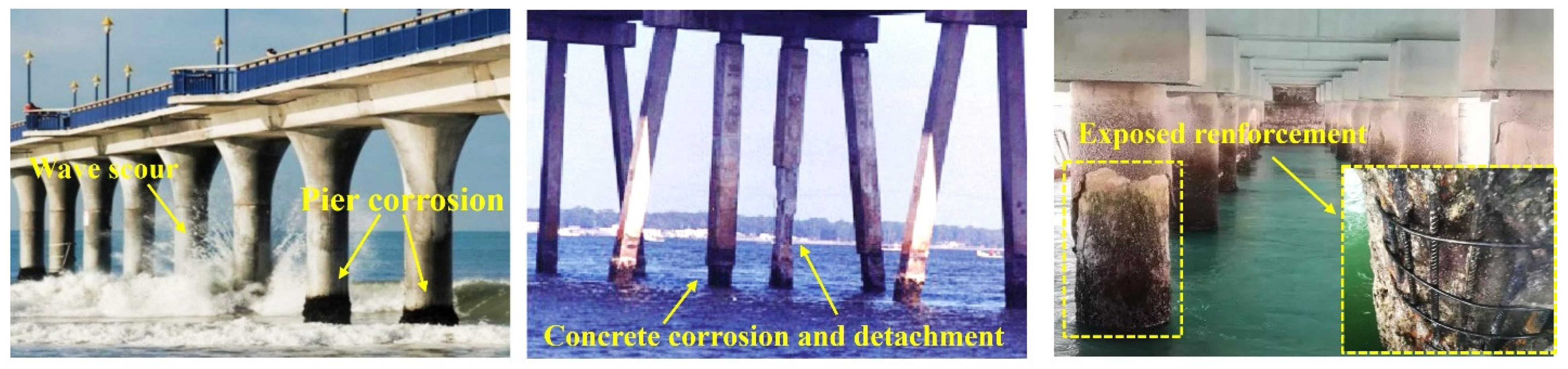
1. Introduction

Sea-crossing bridges, as a key node and important component of the transportation network, play a pivotal role in advancing the development of the marine transportation infrastructure and hold significant strategic importance [1,2,3]. Numerous sea-crossing bridges worldwide have adopted a high-rise pile cap substructure [4], such as the San Francisco Bay Area Bridge in the United States [5], the Akashi Strait Bridge in Japan [6], the Sydney Harbor Bridge in Australia [7], and the Donghai Bridge in China [8]. Unlike land bridges, marine bridges are situated in complex and dynamic marine environments, typically characterized by deep water and large waves [9,10]. Wave action is often one of the key loads influencing the structural design of sea-crossing bridges [11,12]. Deep-water high-rise pile cap foundations are highly flexible and are susceptible to damage from foundation scour and dynamic forces from the water medium. Effectively analyzing dynamic damage has always been a challenge for the safe and healthy operation of sea-crossing bridges.

Bridge structures typically enjoy extended longevity; however, in marine settings, reinforced concrete bridges experience considerable degradation due to environmental elements such as alternating wet–dry conditions, chloride ion corrosion, and carbonation, resulting in a notable decline in their durability [13,14,15]. Among these factors, chloride ion corrosion stands out as a major culprit for reinforcement corrosion as it initiates the deterioration process. This corrosion compromises the concrete’s protective layer, hastening the corrosion of internal reinforcement, consequently diminishing the load-bearing capacity of the bridge components and ultimately culminating in reduced durability [16,17]. As shown in Figure 1, the reinforced concrete column under chloride ion erosion reveals that the rust expansion of the reinforcement leads to the detachment of the protective concrete cover. Additionally, with the increase in service time, the column exhibits a significant occurrence of longitudinal rust spots.

In recent years, researchers both domestically and abroad have investigated the mechanism, rate, and influencing factors of steel reinforcement corrosion through experiments and theoretical models. Yuan et al. [18] accelerated the corrosion rate of steel bars in concrete by adding chloride salt, finding that the cracking of the concrete has a significant effect on the corrosion rate. However, a reasonable model has not been established to simulate the accelerated process of steel bar corrosion after concrete cracking. Ou et al. [19] conducted accelerated corrosion tests on the steel bars of large reinforced concrete beams using the method of applied current, and conducted cyclic load tests on corroded beams. It was concluded that the mass loss of stirrups is greater in the same accelerated corrosion time. As the corrosion progresses, the stirrups fracture, causing the beam to transition from bending failure to bending–shear failure. Akiyama et al. [20] used X-ray digital image processing to visualize the corrosion process in reinforced concrete members to estimate the reliability of these structures. Based on response surface theory and finite element model results, Fan et al. [21] examined the impact of corrosion and erosion on the brittleness of bridge structure barges. It was found that corrosion and erosion have a net positive impact on the dynamic response of the pier columns of sea-crossing bridges and cause greater damage to pile foundations.

While a considerable amount of research has focused on the effects of chloride ion corrosion on the performance and durability of sea-crossing bridges, studies on the dynamic failure processes and long-term mechanisms under wave action remain limited. Given the aging of sea-crossing bridges and the deterioration of their material and structural capacities, investigating fluid–solid coupling and conducting dynamic response analyses of high-rise pile caps under nonlinear pile–soil interactions is of significant importance.

Traditional methods often rely on simplified models and assumptions, such as basic static load analyses or empirical wave force calculations [22,23]. In contrast, this study employs more detailed models that account for the complex impacts of sediment erosion and corrosion, and examines long-term dynamic responses through fluid–solid coupling analysis and pile–soil interaction. In Section 2, the fluid domain model is established based on the wave principle, and the feasibility of the numerical flume is verified. In addition, the modeling process of high-rise pile cap is introduced in detail. A simulation of the scouring effect and the degradation of structural strength due to corrosion are also introduced into the model. Finally, the results of numerical simulation are discussed and analyzed in Section 3. This section includes a discussion of the hydrodynamic analysis of the cap; the degradation of the performance parameters of the structural materials under corrosion; and the energy, displacement, stress, and acceleration response characteristics of the high-rise pile cap. This study provides key insights for early damage warning and guidance on protective measures, enhancing the resilience and durability of marine structures against scour and corrosion.

2. Refined Modeling with Scour- or Corrosion-Induced Effects

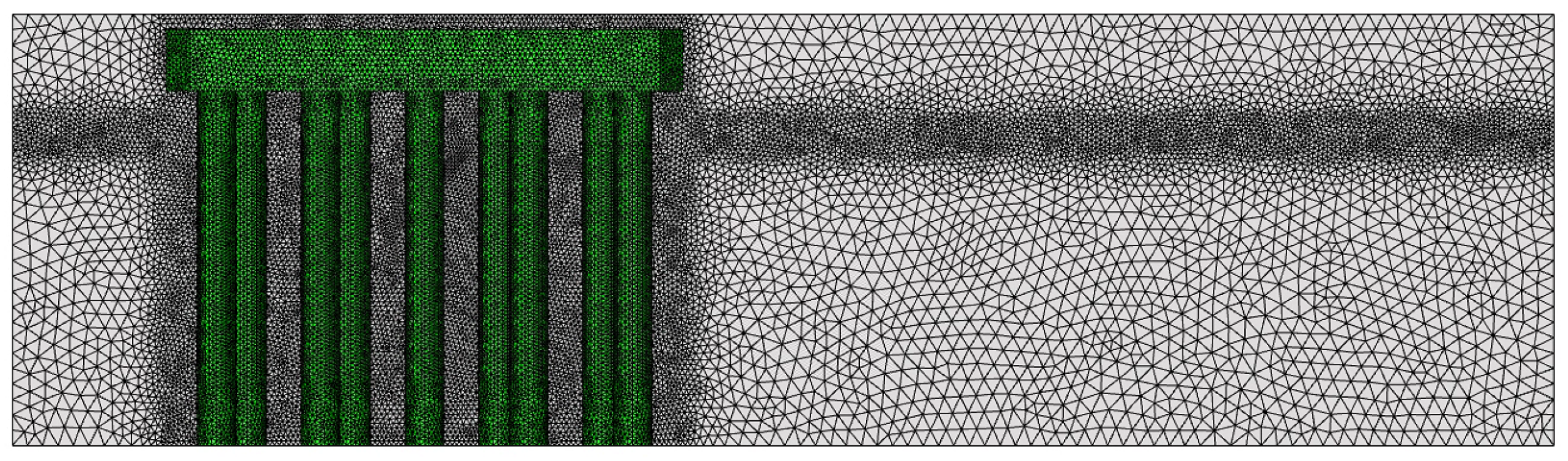
2.1. Fluid Domain Modeling

2.1.1. Governing Equations

When simulating wave motion in the study of wave–structure interactions, it is assumed that water is an incompressible viscous fluid [24,25]. The continuity equation and Reynolds time-averaged Navier–Stokes equation (RANS equation) are used as the control equations for wave motion [26].

$${\displaystyle \frac{\partial }{\partial x_i}}(u_i{A}_i)=0.$$

(1)

$${\displaystyle \frac{\partial u_i}{\partial t}}+{\displaystyle \frac{1}{V_F}}(u_j{A}_j{\displaystyle \frac{\partial u_i}{\partial x_j}})=-{\displaystyle \frac{1}{\rho }}{\displaystyle \frac{\partial p}{\partial x_i}}+G_i+f_i.$$

(2)

where i = 1, 2, 3, x_i represents the x, y, z coordinates; u_i represents the time-averaged velocity in each direction of the flow field; A_i represents the area fraction of the flowable fluid in each direction; V_F represents the volume fraction of the fluid; t represents the time; p represents the fluid pressure; ρ represents the fluid density; G_i represents the gravitational acceleration of the fluid in each direction; and f_i represents the acceleration due to viscous forces in each direction [26], expressed as follows:

$$f_i={\displaystyle \frac{1}{V_F}}[{\displaystyle \frac{{\tau }_{b,i}}{\rho }}-{\displaystyle \frac{\partial }{\partial x_j}}(A_j{S}_{ij})].$$

(3)

$$S_{ij}=-(\begin{array}{c}v+v_T\end{array})[{\displaystyle \frac{\partial u_i}{\partial x_j}}+{\displaystyle \frac{\partial u_j}{\partial x_i}}].$$

(4)

where ${\tau }_{b,i}$ denotes the fluid shear stress in each direction plane; S_ij denotes the strain rate tensor; v denotes the dynamic viscosity; and v_T denotes the turbulent viscosity.

A wave’s free surface must satisfy both dynamic free surface boundary conditions and kinematic boundary conditions, meaning that the normal component of fluid velocity must match that of the boundary itself, and the stress vector component must be continuous [27,28]. Capturing the free surface of waves is crucial in establishing numerical wave flumes. The Volume of Fluid (VOF) method was used to monitor the interface between air and water [29,30,31]; this method defines the volume fraction function α for each phase of the two-phase fluid in every computational cell.

$$\alpha (x,t)=\{\begin{array}{cc}0,& air\\ 1,& water\\ 0<{\alpha }_s<1,& freesurface\end{array}.$$

(5)

Once the volume fraction had been established, the two-phase flow was treated as a mixed-phase fluid, with its density ρ and dynamic viscosity μ expressed as

$$\{\begin{array}{c}\rho =\alpha {\rho }_1+(1-\alpha ){\rho }_2\\ \mu =\alpha {\mu }_1+(1-\alpha ){\mu }_2\end{array}.$$

(6)

The volume fraction function was derived by solving the subsequent equation:

$${\displaystyle \frac{\partial \alpha }{\partial t}}+{\displaystyle \frac{\partial }{\partial x_i}}(\alpha u_i)+{\displaystyle \frac{\partial }{\partial x_i}}[\alpha (1-\alpha )u_{\alpha i}]=0.$$

(7)

where u_i is the relative compression velocity [32], and the final term on the left side of the equation serves as an artificial compression term, aiming to restrict numerical diffusion. α_water = 0.5 is taken for all free liquid levels in the numerical simulations of this study.

2.1.2. Numerical Model Setup

A three-dimensional numerical flume model, measuring 100 m × 54 m × 28 m (length × width × height), was established, as depicted in Figure 2. The design static water depth was set at 20 m. To eliminate the wave attenuation caused by the viscous effects of water and frictional interactions, the left edge of the pile cap was positioned 10 m from the inlet. Employing the boundary wave-making method, the wave-making boundary was set through the velocity inlet. The wave-absorbing region was set in a three-dimensional area within one wavelength at the end of the flume. The bottom and front/rear faces were designated as non-slip wall conditions, while the top face was represented as an atmospheric pressure outlet.

The model was meshed using a computational fluid dynamics (CFD) unstructured mesh; the mesh model is shown in Figure 3. To accurately capture wave motion and free-surface phenomena, grid refinement was applied within 3 m above and below the free surface and in the vicinity of the pile cap region. The global grid size was set at 0.5 m, with a refined grid size of 0.2 m in the specified regions, resulting in a total grid count of 18,684,462 cells. Wave gauges were positioned at 1 m and 10 m from the entrance to monitor the wave generation effects in the numerical flume.

The upper part of high pile cap fluid–structure coupling model is a rectangular pile cap of 3350 cm × 1750 cm × 400 cm. Detailed dimensions are shown in Figure 4. For the sake of esthetics, chamfers of 150 cm × 150 cm were set at the four corners of the pile cap. Since the selected wave conditions in this study do not directly impact the cap, the mitigating effect of the chamfers on wave-induced erosion was not a primary focus of the investigation.

During the computation process, multiphase flow handling was employed, where the fluids considered were gas phase and liquid phase, with their physical property parameters set as shown in

Table 1. Physical properties of fluid.

Fluid Type	Density (kg/m3)	Dynamic Viscosity (kg/m·s)	Linear Attenuation Impedance (s−1)
Air	1.225	1.7894 × 10−5	0
Water	998.2	0.001003	2.0367

. The VOF model was utilized to track the free surface, while the realizable k-ε model was chosen as the viscous model. A segregated solver was selected, with the pressure equation solved using the body-force-weighted method. The pressure–velocity coupling method employed the PISO algorithm, and the volume fraction was calculated using the Geo-Reconstruct method. In the operating environment, the pressure reference value was set to 101,325 Pa and the gravity acceleration was set to 9.81 m/s². Considering both convergence issues and computational time, a time step of 0.05 s was set, and the transient calculation was conducted.

The Stokes second-order wave was used to simulate ocean waves. According to the application range of the wave theory proposed by Maywalt [33], the relevant wave parameters of the Stokes second-order wave were taken in the following ranges:

$$H/g{T}^2\in (0.001~0.0086).$$

(8)

$$H/L\in (0.00625~0.0503).$$

(9)

Here, H is the wave height, g is the gravitational acceleration, and T is the period. The hydrostatic depth was taken as D = 20 m, the wave height was taken as 1.2 m, and the period was taken as 4 s. The wavelength, period, and hydrostatic depth followed a diffuse relationship with each other during wave propagation [34], and the water depth and period of the wave had an effect on the wavelength in the process of wave propagation. Under the condition that the wave period and hydrostatic depth were known, the wavelength L = 25 m was calculated by Newton’s iterative method based on Equation (10) for the wave velocity in finite water depth.

$${\displaystyle \frac{L}{T}}=\sqrt{{\displaystyle \frac{gL}{2\pi }}\tanh {\displaystyle \frac{2\pi D}{L}}}.$$

(10)

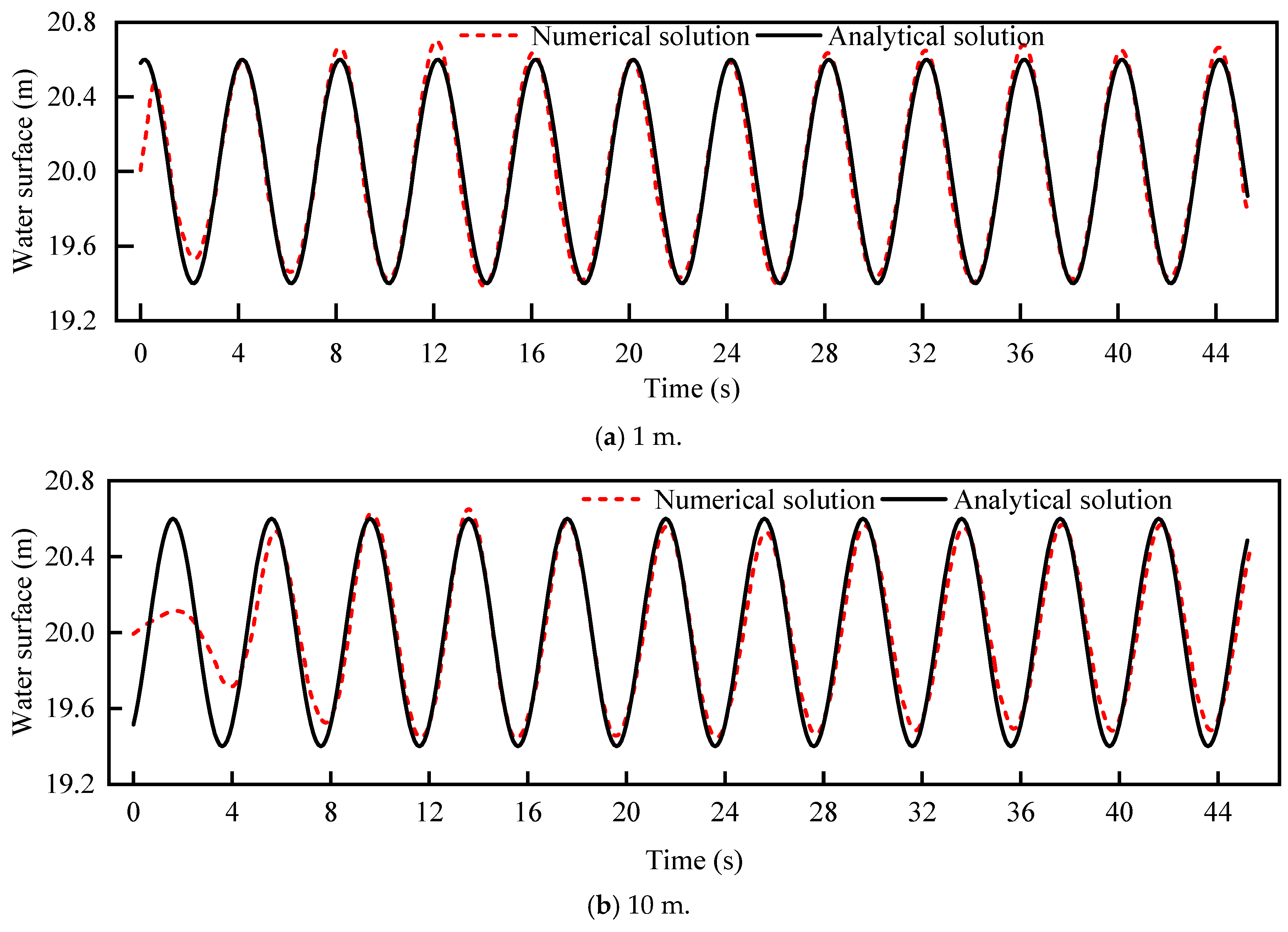
2.1.3. Numerical Wave Verification

The accuracy of the numerical wave simulations in the numerical wave flume needed to be validated primarily through a comparative analysis of the spatiotemporal distribution of waveforms in the numerical wave flume with theoretical waveforms. In the numerical wave flume, wave gauges were set up at positions 1 m and 10 m from the inlet to monitor wave heights over time, which were then compared with the time-domain curves of the theoretical wave heights.

Figure 5 illustrates the variation of wave amplitudes over time at the horizontal wave gauge locations in the numerical wave flume. It can be observed that, during the motion of numerical waves, the ascent and descent of the waves exhibit good periodicity and stability. Once the numerical waves stabilize, their wave period aligns with the theoretical waveform period, and the crest and trough positions are essentially consistent. Comparing the time-domain curves of wave amplitudes at x = 1 m and x = 10 m locations, it is evident that the further the monitoring position is from the velocity inlet, the longer the development time of the waveforms, requiring more time to form stable waveforms. This phenomenon occurs because, at the initial moment, the water at the wave generation boundary undergoes periodic changes based on the wave generation function provided by the Stokes second-order wave. However, since the fluid is not a rigid body, it takes some time for the fluid motion patterns at the wave generation boundary to propagate to the corresponding monitoring positions, thus forming stable waves.

2.2. Solid-Domain Modeling Considering Scour and Corrosion

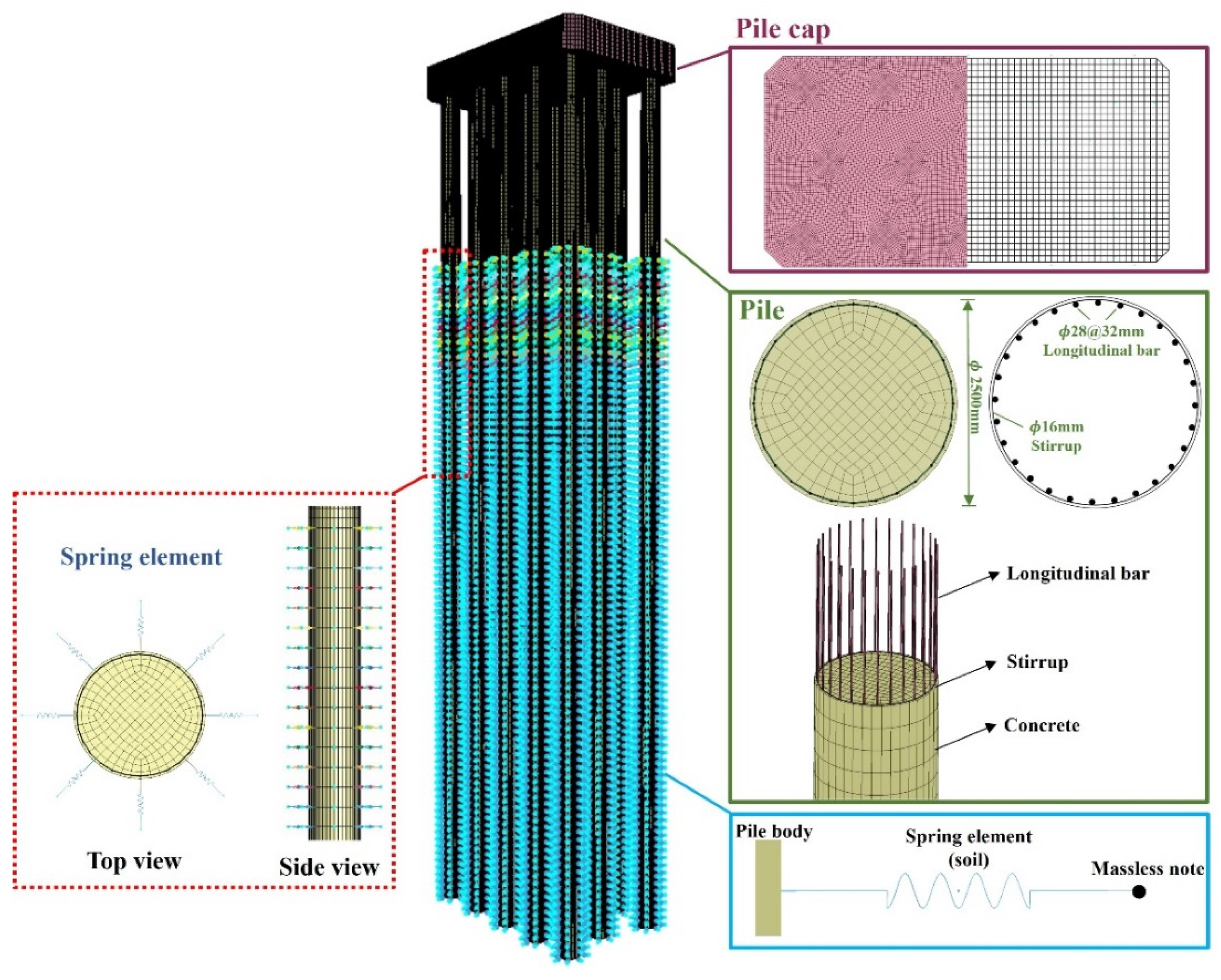
2.2.1. High-Rise Pile Cap Modeling

The high-rise pile cap at the mid-span position of the 1000t-level auxiliary navigation hole continuous beam bridge of the Donghai Bridge was selected as the case analysis object, as shown in Figure 6. The height of the pile was 110 m, and the height of the pier cap was 4 m. The compressive strength of the concrete for the piles and pile cap was 30 MPa. There were 28 longitudinal bars arranged along the circumference of the pile, with a longitudinal bar diameter of 32 mm and a yield strength of 400 MPa. Along the longitudinal direction of the pile, there were 110 stirrups with a diameter of 16 mm and a yield strength of 335 MPa. The concrete protection layer thickness of the bridge pile was 50 mm. The soil depth of the pile was 87 m, and the depth of the seawater was set at 20 m. Based on the corrosion degree, the non-buried segment of the high-rise pile cap structure was divided into three zones: atmospheric area (4 m), wave splash area (3 m), and immersed area (20 m). This setup indicates that the structure is situated in a low-tide marine environment.

A refined model of the high-rise pile cap was established using the dynamic analysis software LS-DYNA (2020) to analyze the long-term dynamic response of the pile cap under different levels of corrosion and scour depth conditions. The material parameters used in this finite element model are shown in

Table 2. Material parameters of high-rise pile cap components.

Component	Element	Constitutive Model	Parameters	Value
Concrete	SOLID	*MAT_CSCM_CONCRETE	Mass density	2400 kg/m3
			Uniaxial compression strength	30 MPa
			Maximum aggregate size	20 mm
			Rate effects	Turn on
Longitudinal bar/stirrup	SOLID	*MAT_PLASTIC_KINEMATIC	Mass density	7850 kg/m3
			Young’s modulus	235,000 MPa
			Poisson’s ratio	0.3
			Yield stress	310 MPa
			Failure strain	0.35
			C	40
			P	5

. Concrete was simulated using the *MAT_CSCM_CONCRETE (159) nonlinear material model, which can effectively simulate the dynamic response behavior of concrete materials. This model was developed by the U.S. Federal Highway Administration. It considers the strain rate effect of concrete materials through Equation (11), which reflects the strain rate characteristics of concrete materials in tensile and compressive cases, respectively, and embodies the enhancement of material strength by the strain rate effect. The model only needs to provide uniaxial compressive strength and maximum aggregate size to automatically generate the relevant parameters.

$$\{\begin{array}{c}{f}_{\mathrm{T}}^{\prime \mathrm{d}}=f_{\mathrm{T}}^{\prime }+E{\epsilon }_e\eta \\ f_{\mathrm{C}}^{\prime \mathrm{d}}=f_{\mathrm{C}}^{\prime }+E{\epsilon }_e\eta \end{array}.$$

(11)

where $f_{\mathrm{T}}^{\prime \mathrm{d}}$ is the dynamic tensile strength of concrete; $f_{\mathrm{T}}^{\prime }$ is the static tensile strength of concrete; $f_{\mathrm{C}}^{\prime \mathrm{d}}$ is the dynamic compressive strength of concrete; $f_{\mathrm{C}}^{\prime }$ is the static compressive strength of concrete; E is the modulus of elasticity; ε_e is the equivalent strain rate; and η is the coefficient of dynamic increase associated with the strain rate parameter.

Steel reinforcement was modeled using the *MAT_PLASTIC_KINEMATIC (003) material [35], a bilinear elastic–plastic material model. The model is based on the elastic–plastic random dynamics model proposed by Cowper and Symonds, which can take into account strain rate effects and cell failure of the material. The Cowper–Symonds eigenequation is

$${\sigma }_d=\left[1+{({\displaystyle \frac{{\epsilon }_r}{C}})}^{1/P}\right]\left({\sigma }_s+\beta E_p{\epsilon }_{eff}^p\right).$$

(12)

where σ_d is the ultimate yield stress; σ_s is the initial yield stress; ε_r is the strain rate; C and P are the strain rate parameters; β is the correction coefficient, where the kinematic reinforcement is taken as 0, and the isotropic reinforcement is taken as 1; E_p is the plastic reinforcement modulus; and ${\epsilon }_{eff}^p$ is the equivalent plastic strain.

The constitutive relationships for concrete and steel reinforcement selected in the numerical model are illustrated in Figure 7. Concrete remains in the elastic deformation stage until it reaches the ultimate load. After exceeding the ultimate load, the decay rate of the concrete’s compressive strength increases rapidly. It is evident that the tensile capacity of the concrete is very limited. Reinforcement exhibits significant elastic–plastic behavior under axial tension. The hardening behavior of kinematic and isotropic reinforcement can be specified by adjusting the modification parameter β.

Additionally, the longitudinal bars and stirrups were discretized using Hughes–Liu beam elements (ELFORM = 1) with a mesh size of 10 mm. The keyword *CONSTRAINED_BEAM_IN_SOLID facilitated perfect bonding between the concrete and steel reinforcement. For the high-rise pile cap, a total of 533,448 solid elements and 134,504 beam elements were employed. Furthermore, to account for the impact of soil resistance on the bridge’s dynamic response, p–y springs (*MATSPRING_INELASTIC) were strategically positioned 45° around the pile and at intervals of 1 m along the pile height to capture the nonlinear soil behavior under wave action, as shown in Figure 8.

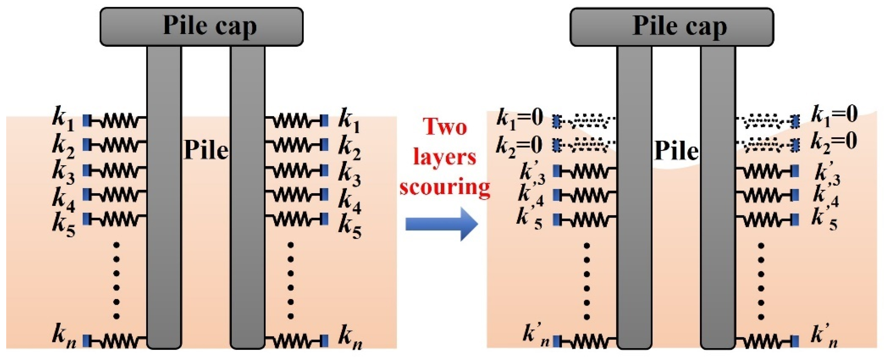
2.2.2. Pile–Soil Interaction Under Scour

In marine engineering, scour pits around pile foundations are formed as a result of wave action on the seabed. The energy from waves induces strong water flow and turbulence in the vicinity of the pile, leading to significant shear forces on the sediment. This process causes the erosion and displacement of seabed sediments surrounding the pile. As sediment is continuously removed due to wave-induced hydrodynamic forces, a localized depression, known as a scour pit, develops and expands over time. It is important to note that scour encompasses not only sediment transport, but also the wear and tear of concrete structures caused by the impact of waves. However, since the latter process occurs at a significantly slower rate, its influence was ignored in this study. The scour pit can compromise the stability of the pile foundation by reducing the lateral support provided by the surrounding soil, potentially leading to uneven settlement or structural instability. Understanding and accurately predicting this scour process is essential for ensuring the long-term stability and safety of marine structures.

The essence of the change in scour depth is the alteration of the pile–soil interaction. Therefore, accurately simulating the variation in bridge boundary conditions was crucial in this study. The soil resistance around the pile group acting on the pile was simplified as a sequence of two-point discrete nonlinear springs, as illustrated in Figure 7. The spring elements adopted the *MAT_SPRING_INELATSIC (MAT_S08) model of non-elastic material, connecting each pile and discrete spring elements spaced at 1 m. Since the soil cannot provide any tensile strength, this model only accounted for compressive response and excluded tensile response. The nonlinear compression stiffness of the springs followed the p–y curve specified in the “Code for Design of Port and Harbour Engineering Pile Foundations” (JTS 167-4-2012) [36,37,38]. The riverbed soil beneath the high-rise pile cap mainly consisted of clay. The depth of the clay was 87 m, its weight density γ was 17.64 kN/m³, and the angle of internal friction α was 35°. The undrained shear strength C_u was 40 kPa.

The calculation formula for the standard value of ultimate horizontal resistance per unit area of clay pile side is

$$P_u=3C_u+\gamma Z+(\zeta C_{u}Z/d).$$

(13)

$$P_u=9C_u.$$

(14)

$$Zr=6C_{u}d/(\gamma d+\zeta C_u).$$

(15)

where P_u represents the standard value of ultimate horizontal soil resistance per unit area of the pile at a depth beneath the mud surface (kPa); C_u represents the standard value of the undrained shear strength of clay in its original state (kPa); γ is the weight of the soil (kN/m³); Z is any depth of the pile below the mud surface (m); $\zeta$ is a coefficient, taken as 0.250~50; d is the pile width or pile diameter (m); and Z_r is the depth at which the ultimate horizontal soil resistance turns (m).

For soft clay with an undrained shear strength standard value less than or equal to 96 kPa, the p–y curve under the non-reciprocating load is determined using the following formula:

$${\displaystyle \frac{P}{P_u}}=0.5{({\displaystyle \frac{Y}{Y_{50}}})}^{1/3}\hspace{1em}\hspace{1em}\hspace{1em}{\displaystyle \frac{Y}{Y_{50}}}<8.$$

(16)

$${\displaystyle \frac{P}{P_u}}=1.0\hspace{1em}\hspace{1em}\hspace{1em}\hspace{1em}\hspace{1em}\hspace{1em}{\displaystyle \frac{Y}{Y_{50}}}\ge 8.$$

(17)

$$Y_{50}=\rho {\epsilon }_{50}d.$$

(18)

where P is the standard value of horizontal soil resistance acting on the pile at a depth below the mud surface (kPa); Y is the transverse horizontal deformation of the pile below the mud surface depth (mm); Y₅₀ is the lateral horizontal deformation of the pile at which the soil surrounding the pile reaches half of its ultimate horizontal soil resistance (mm); ρ is the correlation coefficient, taken as 2.5; and ε₅₀ is the stress value at half the maximum principal stress difference in the triaxial test. For soft clay with high saturation, the strain value at half of the unconfined compressive strength can also be taken. If there are no test data, the value should be taken according to the following rules: if C_u is at 12~24 kPa, ε₅₀ selects 0.020; if C_u is at 24~48 kPa, ε₅₀ selects 0.010; if C_u is at 48~96 kPa, ε₅₀ selects 0.007.

The soil surrounding an individual pile exhibits an infinite state when subjected to external horizontal loads, which means that the response of the soil is assumed to be unaffected by other factors, such as the influence of adjacent structures or boundary effects. However, in a cluster of piles, the proximity between piles alters the p–y curve of the soil surrounding the inner pile foundation, as it experiences reduced horizontal resistance compared to that of a single pile. Conversely, the soil surrounding the outer pile foundation maintains a semi-infinite state, resulting in a p–y curve similar to that of a single pile soil [39]. Therefore, the group pile foundation needs to consider the group pile effect. According to the JTS 167-4-2012, except for the pile farthest from the load point, the pile group effect should be considered for all other pile sections with a center distance of less than 8 times the pile diameter and a depth of less than 10 times the pile diameter. The commonly used method to consider the effect of pile group is to multiply the horizontal soil resistance of a single pile foundation by a reduction coefficient, which can be calculated using the following formula [36]:

$${\lambda }_h={\left({\displaystyle \frac{(S_0/d)-1}{7}}\right)}^{0.043(10-Z/d)}.$$

(19)

where ${\lambda }_h$ is the reduction coefficient of soil resistance; S₀ is the spacing between piles; Z is the arbitrary depth of the pile foundation below the mud surface; and d is the pile diameter.

The p–y curves of the soil layers before and after reduction at each depth, based on the above calculation data, are shown in Figure 9. Guo et al. [40] simulated varying scour depths by removing soil springs at corresponding locations within the scour hole. Although the material parameters of the soil used in their study differ from those adopted here, the variation in stiffness of the nonlinear soil springs with depth follows a consistent trend. Similarly, the reduction in soil spring stiffness due to pile group effects exhibits comparable behavior between the two studies. These findings collectively demonstrate the rationality of the soil spring parameters selected in this work, further validating the robustness of the proposed modeling approach.

When simulating the process of foundation scouring, it is assumed that the actual scouring process is a riverbed soil erosion process and the scour depth of each pile is the same. When scouring occurs, the surface sediment is washed away by the water flow, and the pile body is exposed. The pile foundation at the washed-away soil layer loses transverse constraints. Therefore, when simulating the scouring process, the soil spring within the scouring depth range is removed, so that the transverse horizontal stiffness of the pile foundation within the corresponding range becomes zero. After scouring occurs, the depth of the lower soil layer changes, and the corresponding horizontal stiffness changes. Recalculations should be made to more finely simulate the entire foundation scouring process (as shown in Figure 10).

2.2.3. Structural Strength Deterioration Due to Corrosion

In marine environments, the aging and continuous degradation of reinforced concrete bridges are attributed to several factors, including the ingress of chloride ions, carbonation, temperature, and pollution [41]. This study specifically focuses on high-rise pile cap corrosion induced by chloride ions, while the microscopic electrochemical mechanism and molecular dynamics are not involved.

During the service life of a bridge, chloride ions from seawater continuously penetrate through the concrete protective layer and eventually reach the steel reinforcement. Upon reaching the steel surface, the chloride ions locally disrupt the passivating film surrounding the reinforcement. The sufficient accumulation of chloride ions on the steel surface leads to localized corrosion, with the expansion of corrosion products causing concrete cracking. Generally, the strength of reinforced concrete structures does not significantly deteriorate before the onset of steel corrosion. However, once corrosion initiates, it reduces the strength of both steel and concrete, thereby compromising the load-bearing capacity of the sea-crossing bridge.

(1)

Corrosion initiation time

The bridge pile corrosion process in marine environments does not begin with construction. The duration between the finalization of the bridge piles and the initiation of corrosion follows a specific timeframe. A precise model can be employed to approximate the onset time of corrosion [42,43]:

$$T_i={\displaystyle \frac{c^2}{4D_c}}{\left[er{f}^{-1}\left({\displaystyle \frac{C_0-C_{cr}}{C_0}}\right)\right]}^{-2}.$$

(20)

$$erf(x)={\displaystyle \frac{2}{\sqrt{\pi }}}{\displaystyle {\int }_0^x{e}^{-y^2}}dy.$$

(21)

where T_i is the start time of the corrosion (year); c represents the thickness of the protective layer (cm); D_c denotes the chloride ion diffusion coefficient (cm²/year); C₀ stands for the equilibrium chloride ion concentration on the concrete surface (kg/m³ concrete); C_cr represents the critical chloride ion concentration at the onset of corrosion in kilograms per cubic meter of concrete; and erf is a Gaussian error function.

The parameters D_c, C₀, and C_cr are related to the environment in which the concrete bridge piles are located. The values of these parameters have been studied by many experts and scholars [44,45,46] and are shown in

Table 3. Parameters affecting the corrosion initiation time.

Dc (cm2/s)	C0 (kg/m3)		Ccr (kg/m3)
	Atmospheric Area	Wave Splash Area
2 × 10−8	2.95	7.35	0.9

.

(2)

Degradation of steel bar properties

The corrosion products of steel bars will reduce their own diameter and yield strength. Before T_i, the steel bars remain in their initial state. After T_i, the corrosion of the steel bars is closely related to the corrosion current density [20,47]. After the T_i moment, that is, after corrosion occurs, the degree of corrosion of the steel bars in the same area segment is uniform. The average cross-sectional area of the corroded steel bars A_s and the yield strength of the corroded steel bars f_s can be calculated using Equations (22)–(25) [48,49]:

$$A_s(t)=\left[1-0.01·Q_{corr}(t)\right]A_{s0}.$$

(22)

where A_s0 is the initial cross-sectional area of uncorroded steel bars, and Q_corr(t) represents the percentage of steel mass loss over time and can be determined using the following equation:

$$Q_{corr}\left(t\right)=\left[1-{\left({\displaystyle \frac{D(t)}{D_0}}\right)}^2\right]\times 100.$$

(23)

$$D\left(t\right)=D_0-0.023i_{corr}·t.$$

(24)

where D₀ and D(t) are the initial diameter and remaining diameter of the steel reinforcement. i_corr denotes the corrosion current density of steel bars. According to Akiyama and Frangopol’s suggested values for i_corr [20], the atmospheric area and wave splash area can be taken as 3 μA/cm² and 6 μA/cm², respectively.

The remaining yield strength of the steel bars can be calculated by

$$f_s(t)=\left(1-{\displaystyle \frac{Q_{corr}(t)}{200}}\right)\times f_{s0}.$$

(25)

(3)

Degradation of concrete strength

In this study, it is believed that the strength of the concrete remains unchanged when the crack width of the concrete protective layer reaches 1 mm. The diminished compressive strength of cracked concrete can be assessed as follows [50,51,52]:

$$f_c^{\prime }(t)={\displaystyle \frac{f_{c0}^{\prime }}{1+K{\epsilon }_1(t)/{\epsilon }_{c0}}}.$$

(26)

In the formula, K is the coefficient related to the diameter and roughness of the steel bar (K equals 0.1); $f_{c0}^{\prime }$ denotes the strength of the concrete at the beginning and $f_c^{\prime }(t)$ denotes that after corroded time t; and ${\epsilon }_{c0}$ is the strain at $f_{c0}^{\prime }$. ${\epsilon }_1(t)$. The average tensile strain of the cracked concrete is calculated using the following equation:

$${\epsilon }_1(t)={\displaystyle \frac{b_f(t)-b_i}{b_i}}={\displaystyle \frac{\Delta b(t)}{b_i}}.$$

(27)

Here, b_i represents the width of the undamaged concrete section, while b_f(t) represents the width post cracking. $\Delta b(t)$ can be derived using the following equation:

$$\Delta b(t)=n_{bars}·w_{cr}(t).$$

(28)

where $n_{bars}$ represents the quantity of steel bars within the compression layer. The average crack width of steel bar $w_{cr}(t)$ is derived by [53]

$$w_{cr}(t)=k_w\left[{\delta }_s(t)-{\delta }_{s0}\right]A_{s0}.$$

(29)

Here, k_w equals 0.0575, ${\delta }_{s0}$ denotes the quantity of steel damage necessary for crack initiation, and ${\delta }_s(t)$ serves as a dimensionless damage function, indicating the reduction in the cross-section within the interval of [0~1].

$${\delta }_s(t)={\displaystyle \frac{A_{s0}-A_s(t)}{A_{s0}}}=0.01·Q_{corr}(t).$$

(30)

$${\delta }_{s0}=1-{\left[1-{\displaystyle \frac{R}{D_0}}\left(7.53+9.32{\displaystyle \frac{c}{D_0}}\right)\times {10}^{-3}\right]}^2$$

(31)

Here, R represents the pitting factor, which ranges between 4 and 8 for natural corrosion and between 5 and 13 for accelerated corrosion tests [54].

(4)

Case study of the high-rise pile cap

The steel reinforcement and the concrete exhibit different characteristics of performance degradation in different corrosion zones. Equation (20) is utilized to calculate the corrosion initiation time. In this study, the high-rise pile cap’s steel reinforcement is anticipated to begin corroding after approximately 8 years in the wave splash zone and around 19 years in the atmospheric zone. Subsequently, Equation (23) is applied to calculate the corrosion rate of the steel reinforcement. Based on the above estimated variables, Equations (22)–(31) were employed to determine the degradation curves of the material properties (such as steel reinforcement strength and diameter, concrete strength) over time. Under the specified conditions, the concrete protective layer is projected to develop a crack width of 1 mm at around the 11th year in the wave splash zone and approximately the 28th year in the atmospheric zone. At this moment, it is assumed that the strength of the concrete remains constant throughout the remaining service life.

Figure 11 illustrates the structural degradation caused by corrosion over time in two corrosion areas. From Figure 11a–c, it is evident that the steel reinforcement in the wave splash zone undergoes performance degradation earlier than that in the atmospheric zone, and the degree of degradation is more pronounced compared to the atmospheric zone. Since the steel reinforcement at the pile cap utilizes the same specification, the analysis exclusively focuses on the degradation pattern of the piles’ stirrups located in the wave splash zone. Figure 11f reflects the degradation pattern of concrete. Similar to the steel reinforcement, the time at which the concrete strength starts to decrease is earlier in the wave splash zone compared to the atmospheric zone. However, the decline in concrete strength toward the end period is more pronounced in the atmospheric zone compared to the splash zone. This difference may be attributed to the complexity of reinforcement at the cap. Further fluid–structure coupling analysis was conducted using structural performance data extracted at service times of 8, 50, and 100 years. The performance indicators of steel reinforcement and concrete for different regions and years are presented in

Table 4. Time-varying parameters considering non-uniform corrosion.

Area	Parameters	Service Time
		8 Years	50 Years	100 Years
Wave splash area	Corrosion rate of steel bars	0	32.94%	63.61%
	Residual diameter of steel bars	32 mm	26.2 mm	19.3 mm
	Yield strength of steel bars	400 MPa	334.11 MPa	272.78 MPa
	Residual diameter of stirrups	16 mm	10.2 mm	3.3 mm
	Stirrup yield strength	335 MPa	235.63 MPa	174.64 MPa
	Concrete strength	30 MPa	10.34 MPa	10.34 MPa
Atmospheric area	Corrosion rate of steel bars	0	12.92%	31.88%
	Residual diameter of steel bars	32 mm	29.86 mm	26.41 mm
	Yield strength of steel bars	400 MPa	374.16 MPa	336.24 MPa
	Concrete strength	30 MPa	9.0 MPa	9.0 MPa

.

Fan et al. [35] employed a comparable model to investigate the corrosion-induced degradation of reinforced concrete bridges. Their results indicated that the initiation of steel corrosion in the splash-tidal zone and atmospheric zone occurred at 8 and 18 years, respectively, which aligns closely with the predictions of this study (8 and 19 years). Furthermore, the time-dependent corrosion behavior of both steel and concrete, as well as the resulting structural deterioration trends, exhibit remarkable consistency between the two studies. These comparative analyses substantiate the validity and reliability of the corrosion degradation model adopted in this work, demonstrating its capability to accurately simulate the long-term corrosion behavior of reinforced concrete structures.

These findings can advance the design and maintenance of coastal infrastructure in corrosive environments by enabling the development of predictive corrosion management approaches, zone-specific protection strategies, and advanced corrosion-resistant materials. Overall, this research offers practical guidance for improving the resilience and sustainability of coastal infrastructure in corrosive environments.

3. Numerical Simulation Results

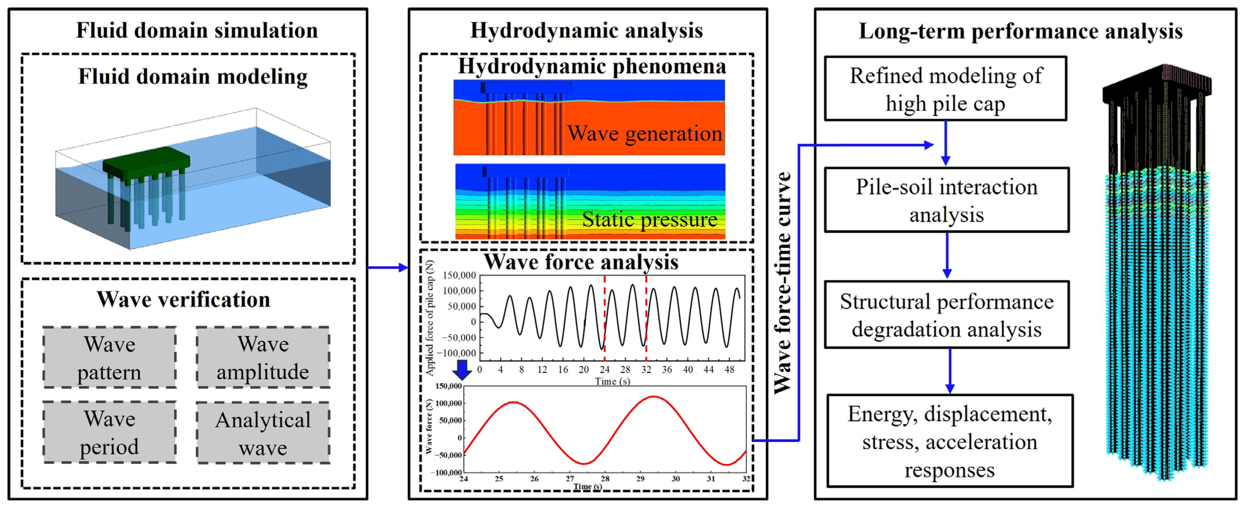
3.1. Analysis Strategy and Process

In the finite element modeling approach, numerical experiments were conducted as follows. In this study, wave parameters with a water depth of 20 m, a wave height of 1.2 m, and a period of 4 s were selected to extract the characteristics of wave forces. High-rise pile cap structures were subjected to three corrosion durations: 8 years, 50 years, and 100 years. Additionally, five local scour depths were considered: 0 m (pristine state), 3 m, 6 m, 9 m, and 12 m (maximum scour depth). In this study, the selection of the scour depth range referred to the empirical formula and the measured scour depth of the bridge site. Johnson et al. [55] introduced a model correction coefficient λ_s to consider the influence of uncertainty on the scour depth of the foundation. The adjusted HEC-18 formula can be expressed as follows:

$$y_s=2.0{\lambda }_s{y}_0{K}_1{K}_2{K}_3{K}_4{\left({\displaystyle \frac{a}{y_0}}\right)}^{0.65}{\left({\displaystyle \frac{V_0}{{\left(g{y}_0\right)}^{0.5}}}\right)}^{0.43}.$$

(32)

where K₁, K₂, K₃, and K₄ are the correction coefficients of pile foundation shape, angle of attack, flow field condition, and sediment particle size, respectively. K₁ = K₂ = K₄ = 1.0, K₃ = 1.1. The value of λ_s is 0.8. y₀ denotes the water depth upstream, g denotes the acceleration of gravity, and a denotes the width of the pier perpendicular to the flow direction.

In this work, the HEC-18 method was used to estimate the scour depth of the Donghai Bridge, in service for 100 years, to be 23 m. In 2020, it was reported that the average depth of the scour holes under the pier of the 17-year-old Donghai Bridge varied between 4 and 7 m, and the deepest was close to 20 m. Therefore, the scour depth was set to 0~12 m with an interval of 3 m. Here, 0 m represents intact state, 3 m and 6 m represent moderate scour, and 9 m and 12 m represent severe scour. Using nonlinear time history dynamic analysis, the study examined the temporal evolution of energy, displacement, stress, and acceleration of the high pile cap across the combinations of these parameters (three corrosion times and five scour depths). Note that the uncertainty of the corrosion and scour rate have not been considered here, and deserve attention in further study.

To facilitate the application of wave loads and improve computational efficiency, the resultant wave force from seconds 24 to 32 obtained through CFD analysis was applied to the high-rise pile cap structure. The LS-DYNA model applies the wave force to the relevant nodes through the *LOAD keyword. It is evident that the wave force is derived from two wave cycles, with a maximum positive resultant wave force of 119,712.5 N and a maximum negative resultant wave force of −77,618.4 N.

An implicit dynamic analysis procedure was adopted to investigate the dynamic response within eight seconds. The analysis process is outlined as follows and shown in Figure 12.

(1)

Conduct a hydrodynamic analysis of the high-rise pile cap using ANSYS-FLUENT software (2022 R1) and extract the resultant wave force from two cycles within the 24–32 s duration;

(2)

Apply the extracted resultant wave force as nodal forces to the corresponding nodes of the high-ride pile cap model established in the LS-DYNA software;

(3)

Consider the performance degradation indicators of concrete, steel reinforcement, and stirrups of the high-rise pile cap at service times of 8, 50, and 100 years;

(4)

Calculate the dynamic stiffness of nonlinear soil springs along the pile axis and simulate scour effects by varying the number of soil springs, considering scour depths of 0 m (pristine), 3 m, 6 m, 9 m, and 12 m;

(5)

Extract dynamic responses such as stresses and the displacements of the high-rise pile cap to analyze its failure behavior.

3.2. Hydrodynamic Analysis

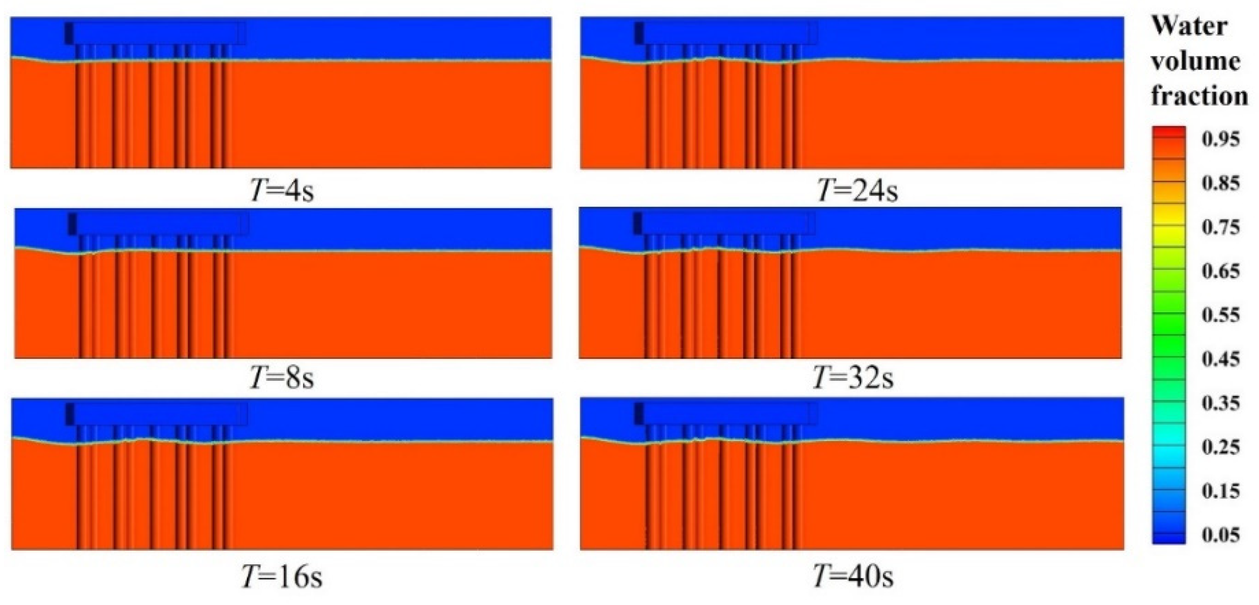
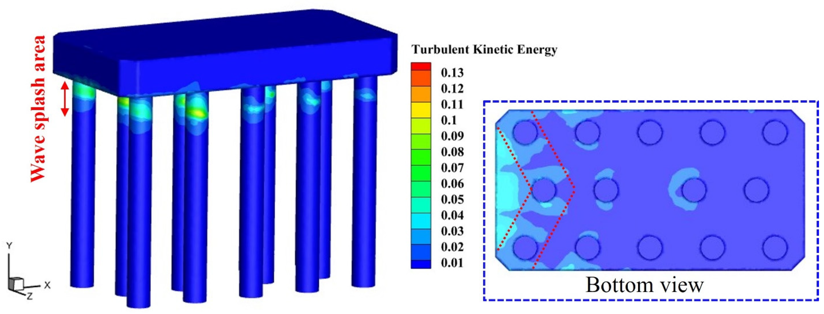
3.2.1. Hydrodynamic Phenomena

Under the wave parameter setting of wavelength L = 25 m and wave period T = 4 s, the wave propagation speed is 6.25 m/s. The whole length of the numerical flume is 100 m. Therefore, in an ideal case, starting from the initial time, after 16 s, the fluid at the wave-making boundary can propagate to the wave-absorbing area at the end of the flume, and then the whole flume forms a periodic and stable wave field. However, due to the obstruction of the pile groups and the viscosity of water, the wave propagation lags behind. Finally, the wave stabilization time appears after 24 s. Figure 13 shows the wave generation process in the numerical flume.

Figure 14 shows a static pressure cloud diagram of the numerical flume under the static water state and the wave motion state. The pressure distribution in the still water state is stratified, and the maximum pressure value at the bottom of the pool is roughly consistent with the theoretical pressure value obtained by the still water depth of 20 m. In the state of wave motion, on the same horizontal line, the water depth at the peak position is greater than the water depth at the trough position, so the net water pressure at the peak position is greater than the net water pressure at the trough position. With the increase in the water depth, the increasing pressure trend is consistent with the theoretical value. The pressure variation occurs primarily within the range of the wave height.

Turbulent kinetic energy reflects the intensity of fluid motion within turbulent regions and also signifies the transfer of energy within the fluid. During the development of turbulence, energy from the high-pressure region is transferred through turbulence to the low-pressure region, thereby redistributing the energy. Figure 15 illustrates the distribution of turbulent kinetic energy on the coupled fluid–structure interface at 32 s. Turbulent kinetic energy tends to concentrate predominantly within the wave splash zone, while other regions exhibit minimal turbulence. Additionally, the presence of group piles notably impacts the distribution of turbulent kinetic energy, resulting in lower turbulence being observed in the back compared to the front row. From the bottom view, it is evident that turbulence exists at the base of the platform, primarily distributed on the windward side. Consequently, under wave action, the wave splash zone and the base of the high-rise pile cap are more susceptible to damage.

3.2.2. Wave Force Analysis

Analyzing the horizontal and vertical wave forces acting on a high-rise pile cap provides valuable insights into the nature of these forces. By integrating the fluid compressive stress and shear stress along the contact surface between the cap and the water, the resultant wave force exerted on the cap can be determined.

Figure 16 displays the temporal evolution of wave forces acting on the cap during wave action. According to Figure 16a, the horizontal wave force exhibits clear periodicity, and positive and negative wave forces are asymmetric. After 12 s, the fluctuation amplitude of the horizontal wave force maintains a stable value. The maximum positive horizontal wave force reaches 144,391.8 N, while the maximum negative horizontal wave force is registered at −149,788 N. As can be seen from Figure 16b, the vertical wave force displays a somewhat periodic pattern, although its periodicity is less pronounced compared to the horizontal wave force. At each wave summit, the wave force experiences varying degrees of sudden fluctuations, primarily because of the instantaneous reversal of the cap’s action on the vertical wave force. When the wave summit impacts the high-rise pile cap, this abrupt reversal leads to an instantaneous surge in the vertical wave force. This phenomenon is particularly evident at 21 s, when the vertical wave force reaches its maximum value of 27,037.14 N.

As depicted in Figure 16c, the resultant wave force exerted on the high-rise pile cap demonstrates clear periodicity, suggesting that the cap’s response to wave loads is predominantly influenced by the horizontal wave force aligned with the wave propagation direction. In comparison, the vertical wave force contributes relatively insignificantly to the resultant force. The maximum positive and negative resultant forces are 119,712.5 N and −88,255 N, respectively, which are lower than the peak value of the horizontal wave forces. This can be attributed to the phase difference between the variations in the horizontal and vertical forces. In the subsequent fluid–structure coupling analysis, the resultant wave force from 24 s to 32 s was selected for application on the high-rise pile cap structure.

The wave force of different wave conditions on high pile caps was not explored further in this study. Xu et al. [56] explored the influence of wave height on high pile caps through experiments, showing that when the wave height exceeds 0.18 m, the horizontal force increases with the increase in the wave height, and the vertical force increases first and then decreases, except for the case of complete submergence. The resultant wave force obtained from this simulation will be used as an external excitation load applied to the finite element model of the high pile cap.

3.3. Long-Term Performance Analysis

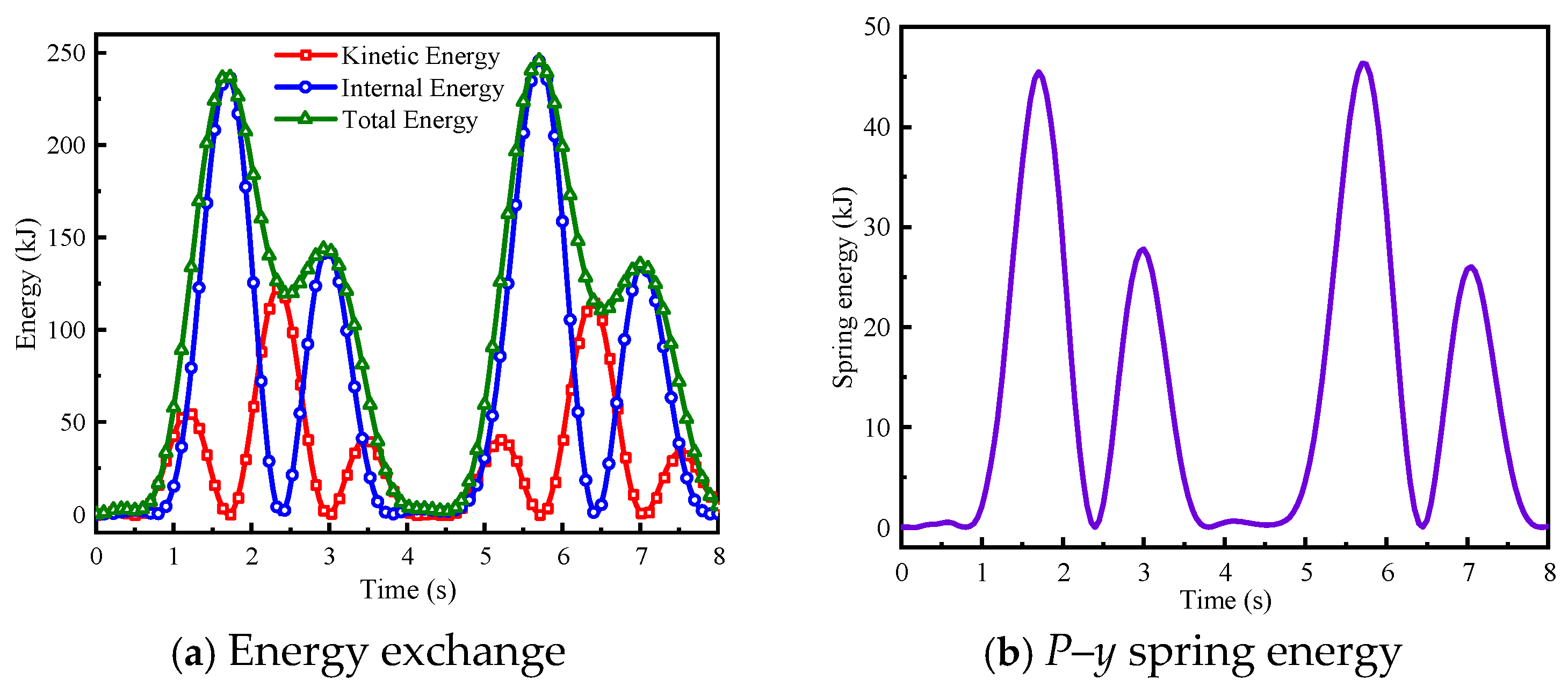
3.3.1. Energy Analysis

Considering the high-rise pile cap and the p–y soil spring as a structural system, this study focuses on investigating the energy changes of the whole system. The energy change in the spring is also included in the change in the internal energy of the structural system. In addition, the damping effect of the system is not considered due to its negligible influence compared to other mechanical properties such as stiffness or mass. The total energy E_total is the sum of all of the energies in the model, the kinetic energy E_kinetic is the energy of all of the moving parts of the model, and the internal energy E_internal is the energy caused by the deformation of the material. The equations are as follows:

$$E_{\mathrm{total}}=E_{\mathrm{kinetic}}+E_{\mathrm{internal}}.$$

(33)

$$E_{\mathrm{kinetic}}={\displaystyle \frac{1}{2}}\sum _i{m}_i{v}_i^2.$$

(34)

$$E_{\mathrm{internal}}={\displaystyle \frac{1}{2}}\sum _i{\sigma }_i{\epsilon }_i$$

(35)

where m_i is the mass of the ith mass point, v_i is the velocity of the ith mass point, σ_i is the stress of the ith cell, and ε_i is the strain of the ith cell.

The changes in kinetic energy, internal energy, and total energy of the high-rise pile cap under wave action were analyzed and recorded. The structure with a corrosion time of 8 years and a scour depth of 12 m was selected to study its energy conversion law, as shown in Figure 17a. It can be found that the period of energy change is consistent with the period of wave load, and the period is 4 s, which means that the energy change in the high pile cap structure is mainly caused by external load. In two cycles (8 s), the change curve of each energy is the same. In the first second of each period, the value of kinetic energy, internal energy, and total energy is 0, indicating that the wave load has not caused the structure to deform during this period. In the process of energy conversion, it can be found that the sum of the internal energy and kinetic energy of the structure at each time point is equal to the total energy, which conforms to the law of energy conservation of the structure. This indicates that the energy change caused by the elastic–plastic deformation of the pile cap is equivalent to the change in internal energy. The internal energy of the structure reaches zero at 2.5 s and 6.4 s, while the kinetic energy peaks at 125 kJ during those instances. At this time, the total energy of the structure is equal to the kinetic energy, which indicates that the structure has entered a very dangerous time. Hence, appropriate measures should be taken to reduce the occurrence of all internal energy converted into kinetic energy.

Figure 17b shows the energy change in the p–y soil spring. The variation law of spring energy is similar to that of structural internal energy. The spring energy value is much smaller than that of internal energy, which indicates that the soil spring gives good restraint and support to the high pile cap under the action of waves. The nonlinear change in spring energy also implies the nonlinearity of structural dynamic response, which lays the foundation for the following dynamic analysis. By comparing the spring energy and internal energy changes in Figure 16, it is evident that the internal energy change induced by deformation contributes more significantly to the overall energy change in the structure.

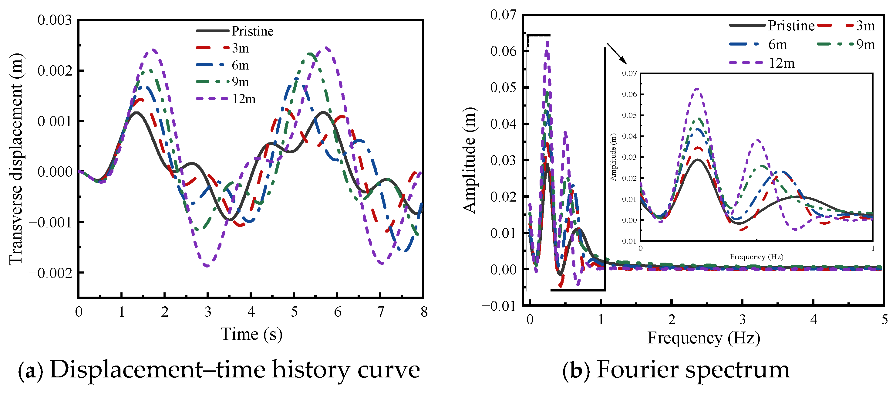
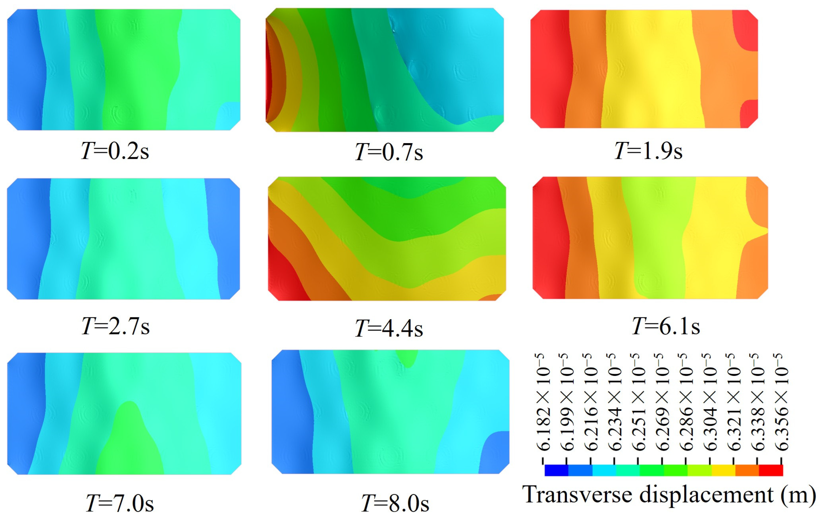
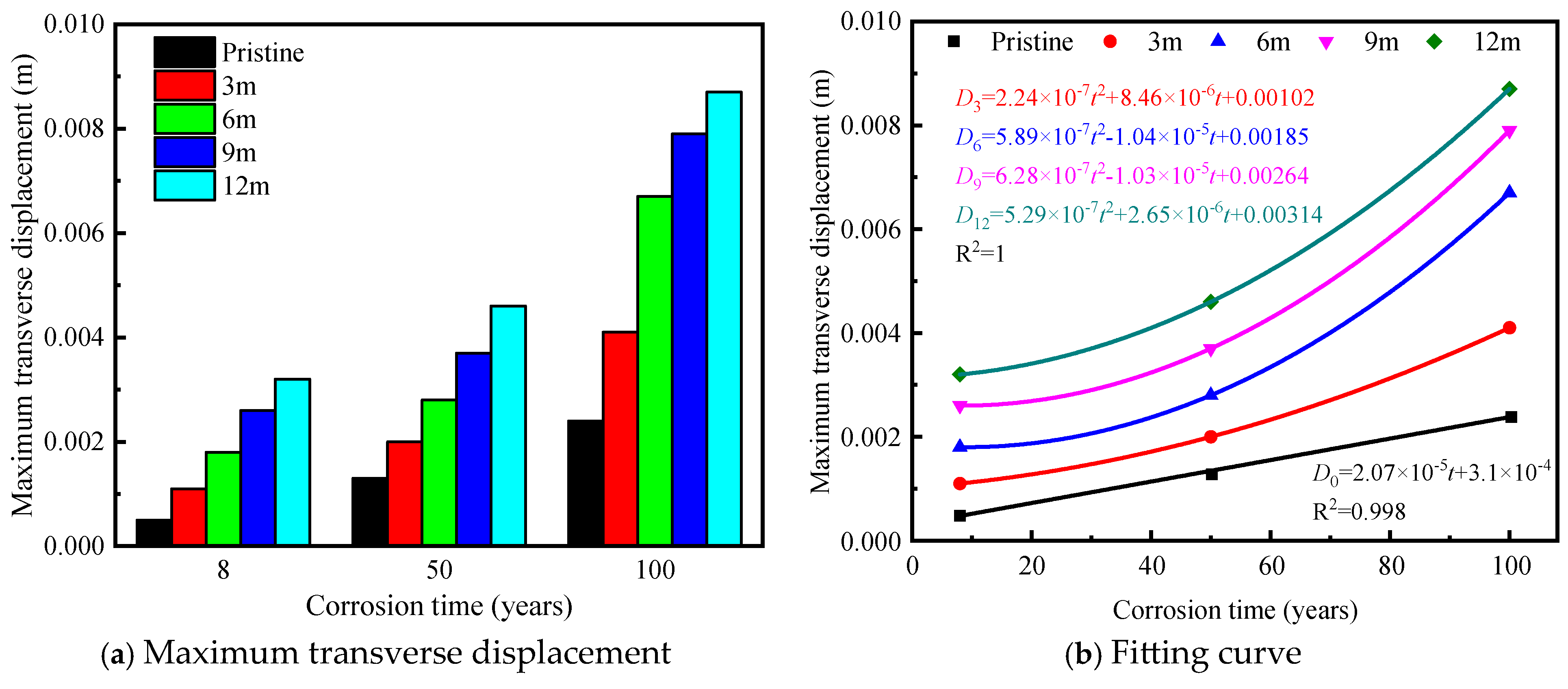
3.3.2. Displacement Response Analysis

The transverse displacement of the cap was calculated under the action of waves. The high-rise pile cap model corroded for 8 years was selected for the comparative study. Figure 18a shows the time history curve depicting the overall transverse displacement of the cap as the wave load time varies across five different scouring conditions. It can be seen that the cap is roughly periodic under the action of wave load, and the transverse displacement increases first and then decreases in a period, which corresponds to the periodicity of the selected wave load. As the scour depth increases, the transverse displacement of the cap also rises accordingly. When the scour depth is 12 m, the transverse displacement value reaches the maximum, which is 0.0025 m. It can also be found that with the increase in the scour depth, the time of maximum transverse displacement is obviously delayed, which may be caused by the redistribution of the stiffness of the remaining nonlinear soil spring after scouring.

Figure 18b shows the Fourier analysis of the transverse displacement of the cap. The first two order frequencies of the cap under five kinds of scouring conditions are less than 1 Hz. The amplitude of the transverse displacement under the first-order frequency is 0.029 m, 0.035 m, 0.043 m, 0.049 m, and 0.062 m with the increase in the scour depth. Obviously, under the same external load, the pile cap with greater scour depth is more likely to be damaged.

Figure 19 shows a transverse displacement cloud diagram of the cap that has been in service for 8 years in two cycles (0–8 s) under the condition of a scour depth of 6 m. Through these cloud images, it can be seen that the maximum transverse displacement occurs near 1.9 s and 6.1 s. In the process of bearing wave load, the displacement of the pile cap is continuous and gradual, which is due to the constraint and bonding effect of the steel bar inside the pile cap.

Similarly, the study focused on the high-rise pile cap that had been in service for 8 years, with a scour depth of 6 m. The displacement–time curves of the top of 14 piles were extracted for analysis, as depicted in Figure 20. Figure 20a–d illustrate the transverse displacement, longitudinal displacement, vertical displacement, and combined displacement of the top of the 14 piles, respectively.

It can be seen from Figure 20a–c that the displacements in all three directions exhibit roughly periodic behavior, following the cyclic variation of wave loading. Among the three directions, there are no significant differences in the transverse displacement of the pile top, indicating good coordination in transverse deformation for the high-rise pile cap with a group pile system. The magnitude of transverse displacement is much larger than that of longitudinal and vertical displacement, suggesting that, of the three directions, transverse displacement has the greatest impact on the deformation of the high-rise pile cap structure. A closer inspection of the local magnification of Figure 20a reveals that the transverse displacement of piles located in the middle (#3, #12) is slightly larger compared to the others, indicating the need for the enhanced monitoring and maintenance of central piles during service.

Figure 20b illustrates the variation pattern of longitudinal displacement at the pile tops. It is evident that, during the first cycle, there is no significant change in the longitudinal displacement of the pile tops, but in the second cycle, the displacement values noticeably increase, with pile #14 showing the most prominent variation. Due to the interaction between longitudinal reinforcement and stirrups inside the piles, there is a lag phenomenon in the variation of longitudinal displacement at the pile top. The longitudinal displacement variation of the piles on the left side of the longitudinal bridge (#4, #5, #8, #9, #13, and #14) precedes that of the piles on the right side (#1, #2, #6, #7, #10, and #11).

Figure 20c presents the variation in the vertical displacement at the pile top. The top vertical displacement in the middle piles (#3 and #12) remains almost unchanged, indicating that wave loading has little effect on the vertical displacement of the piles in the middle. Additionally, it is noted that the variation pattern of the vertical displacement on the left side of the longitudinal bridge is completely opposite to that of the piles on the right side. The top vertical displacement at piles #4, #5, #8, #9, #13, and #14 increases first and then decreases within one cycle, while for piles #1, #2, #6, #7, #10, and #11, it decreases first and then increases. The variation in the vertical displacement of piles near the edge is much greater than for those in the middle and near the middle.

Figure 20d illustrates the resultant displacement–time curve of the piles. The variation pattern of resultant displacement for the 14 piles is roughly the same, once again confirming that transverse displacement has the most significant influence on the deformation of the high-rise pile cap structure. The resultant displacement values within two cycles are all greater than zero, indicating that, under unidirectional wave action, the high-rise pile cap tends to offset in the direction of wave propagation.

To further investigate the relationship between the increasing longitudinal displacements and potential resonance, we conducted a Fourier analysis on the longitudinal displacement at the top of pile #7, as shown in Figure 20e. The maximum longitudinal displacement at the first natural frequency (0.6 Hz) is 1.52 × 10⁻⁵ m. Notably, the longitudinal displacements induced by wave are significantly smaller than this value. Therefore, the gradual increase in longitudinal displacement is attributed to the cumulative effect of wave-induced displacements rather than resonance.

Figure 21a shows the maximum transverse displacement of pile top #1 under different scour depths for 8 years, 50 years, and 100 years. It can be seen from the histogram that as the corrosion time increases, the maximum top transverse displacement of the pile gradually increases. Upon reaching the bridge’s service time limit, the maximum top transverse displacement of the pile is greater under various scour conditions compared to other corrosion periods. It can be concluded that when the service time and scour depth increase, the substructure of the sea-crossing bridge should be repaired and protected in time.

Figure 21b illustrates the relationship between the maximum transverse displacement of pile #1 and the duration of corrosion at various scour depths through a fitted analysis. The fitted values of maximum transverse displacement and corrosion duration are displayed in the figure. A correlation coefficient greater than 0.95 indicates that the empirical formula fits accurately. When scour damage is absent, there is a nearly linear correlation between displacement and corrosion duration. As the scour depth increases, the relationship between transverse displacement and corrosion duration follows a nonlinear quadratic polynomial. Moreover, the displacement values increase exponentially with longer corrosion durations. Consequently, as the service life of a sea-crossing bridge extends, timely scour protection and material maintenance are crucial.

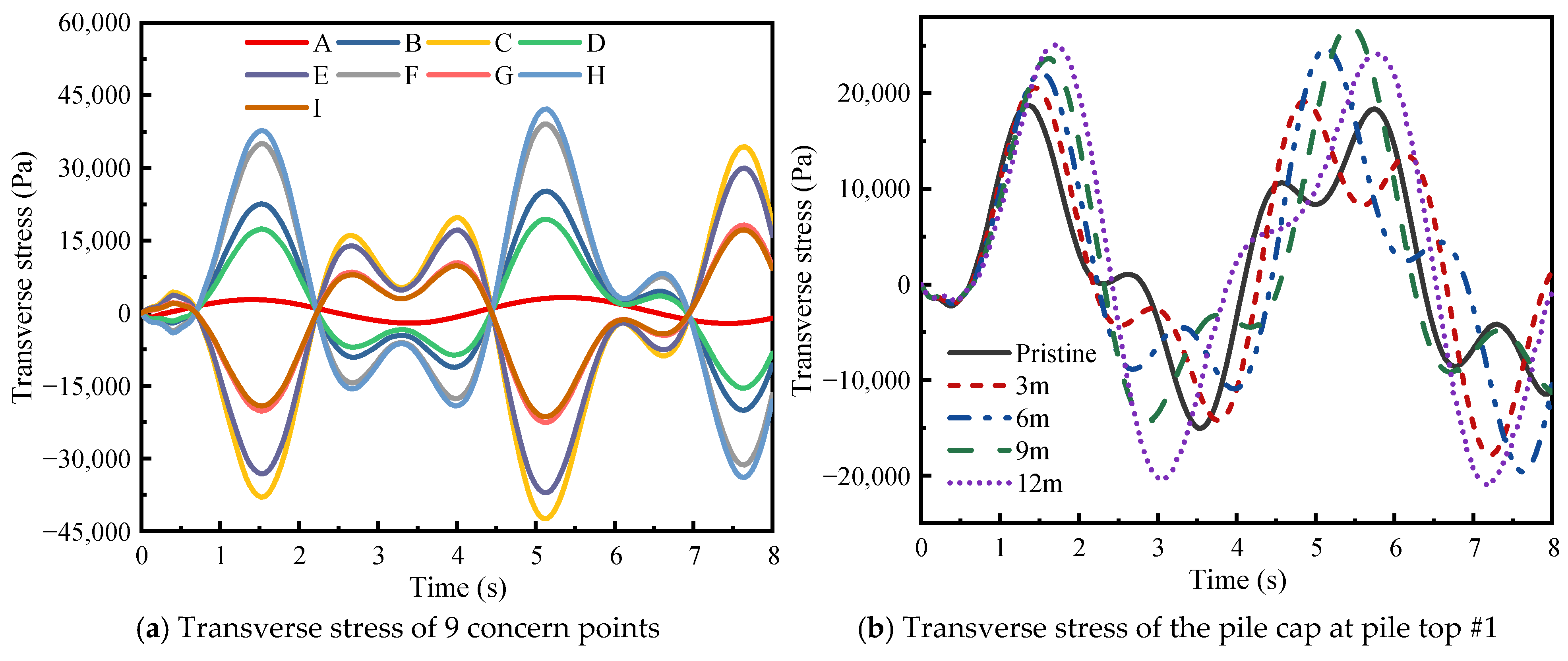
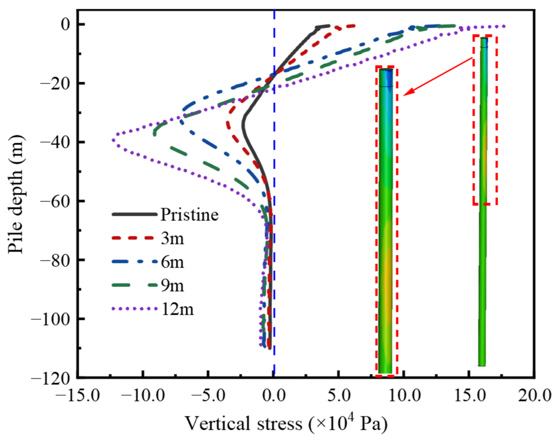
3.3.3. Stress Response Analysis

Nine points of concern were selected in the middle of the bottom of the cap to explore the variation law of the stress of the cap. As shown in Figure 22, the nine points of concern are respectively displaced at the middle edge of the cap bottom and the two sides of the pile cap connection. The relationship between the transverse stress and time of each concern is shown in Figure 23a. It can be seen that the stress at the edge shows a good period consistent with wave load. Although the cap edge will be in direct contact with the wave, the stress value is smaller than other concerns at the pile cap connection. The stress change trend on the left side of the pile (concern points C, E, G, and I) is opposite to that on the right side of the pile (concern points B, D, F, and H). Moreover, as the distance from the edge of the cap increases, the maximum amplitude of the transverse stress gradually decreases. The curve of the transverse stress of the pile cap at pile #1 with different scour depths was extracted, as shown in Figure 23b. With the increase in the scour depth, the variation amplitude of transverse stress shows an increasing trend. In the first cycle, when the scour depth reaches 12 m, the maximum transverse tensile stress is 25,020.52 Pa, and the maximum transverse compressive stress is 20,225.61 Pa. Moreover, with increasing scour depth, there is a delay in the occurrence of maximum transverse stress at this location, which indicates that a larger transverse displacement will occur.

Similarly, the high-rise pile cap with a corrosion time of 50 years was selected as the research object, and the vertical stress distribution along the pile body at 5.8 s of pile #1 under different scour conditions was extracted (Figure 24). The distribution of vertical stress is observed along the depth direction of the pile. There is vertical tensile stress at the pile top, and vertical compressive stress at the depth of 35 m. For reinforced concrete structures, where tensile stress exists, concrete is more likely to be destroyed, so it is necessary to increase the arrangement of steel bars at the pile cap connection. Below the buried depth of 60 m, the vertical stress value of the pile is very small and only compressive stress is exerted, so the pile in this area is not easily damaged. With the increase in the scour depth, the vertical tensile/compressive stress values at the pile top at the buried depth of 35 m gradually increase, so monitoring sediment scour is crucial to increase the service life of piles.

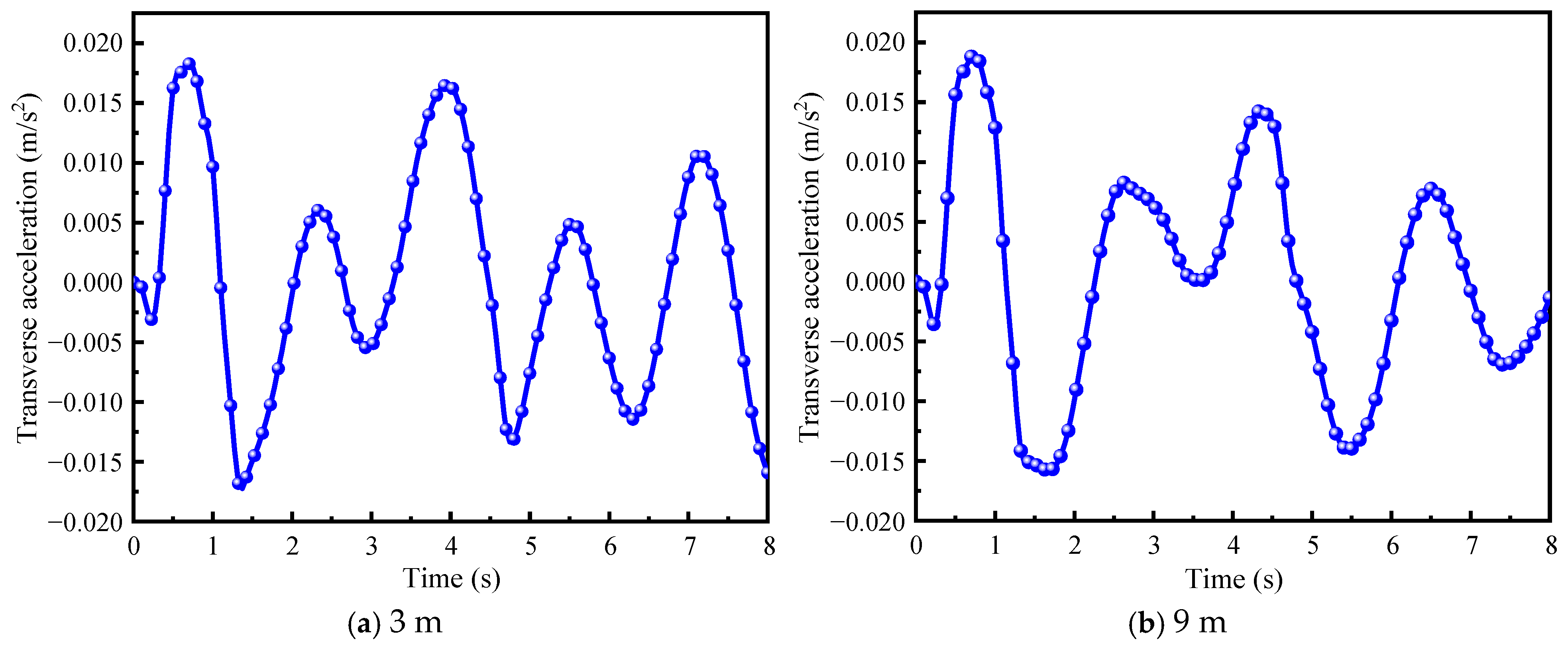
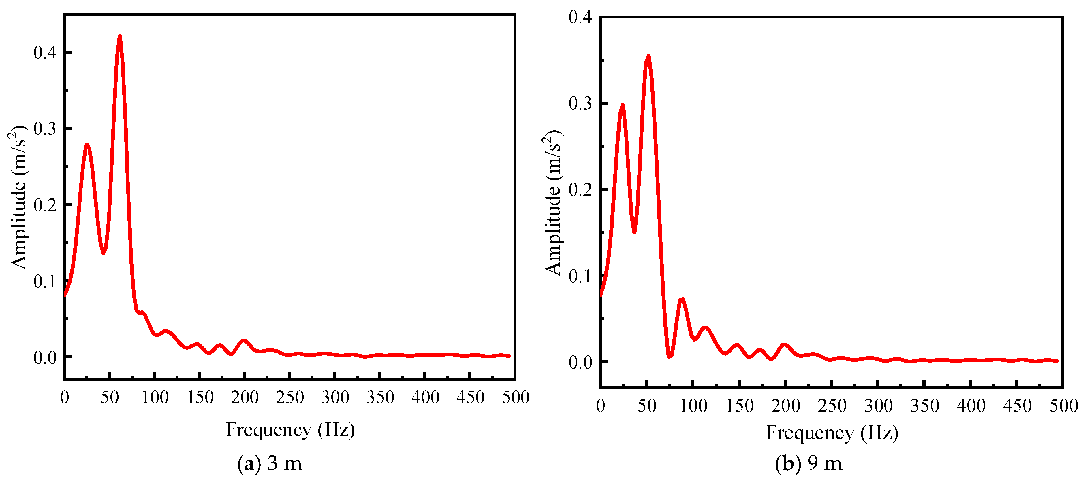
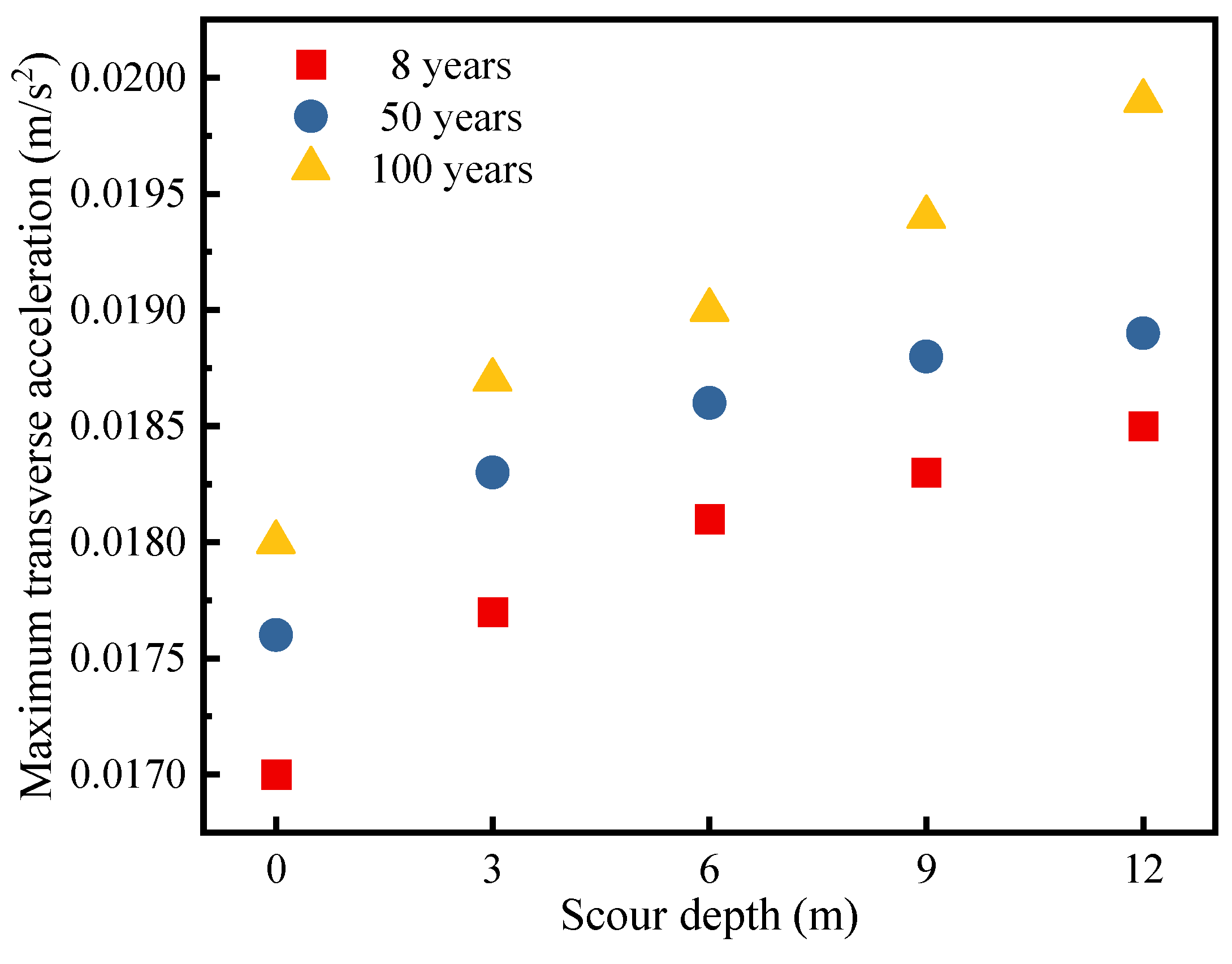
3.3.4. Acceleration Response Analysis

The high-rise pile cap with a corrosion time of 50 years was taken again as the research subject, and the transverse acceleration time history curves of the cap at scour depths of 3 and 9 m were extracted, as shown in Figure 25. When a wave load acts on the structure, the acceleration of the cap changes abruptly, and the maximum positive acceleration and the maximum negative acceleration are roughly equal. When the scour depth is 9 m, the peak acceleration time is longer than that at 3 m. This is due to the decrease in nonlinear spring caused by the increased scour depth, which affects the overall stiffness of the structure.

Figure 26 shows the frequency characteristics of the acceleration, which were extracted from the acceleration response using fast Fourier transform (FFT). Two main frequency bands can be identified from the acceleration spectrum analysis results of the cap under 3 m and 9 m scour depths. The two main frequency bands are the same: 0–50 Hz and 50–75 Hz, respectively. The 0–50 Hz frequency range typically includes low-frequency vibration modes that reflect the fundamental dynamic response of a structure. For bridges or large structures, these low-frequency modes are often linked to overall stability and long-term performance. In contrast, the 50–75 Hz range usually encompasses higher-frequency modes, which may relate to the local vibration characteristics of the structure. Within this region, the structure can display complex vibration behaviors, including higher-order modes, which can significantly impact its dynamic response.

In practice, engineers use established experience and theoretical knowledge to identify key frequency bands, with the 0–50 Hz range generally corresponding to the structure’s fundamental frequency and the 50–75 Hz range possibly involving higher-order vibration modes. Within the frequency range of 0–50 Hz, the predominant frequency is 25 Hz, corresponding to 100 times the frequency of the incident wave. However, the acceleration assignment in each frequency band is different. The main vibration frequency of the structure is the second-order frequency of 62 Hz. The general rule is that the maximum acceleration assignment under 62 Hz is greater than that under 25 Hz, which also explains why the dynamic response of the structure is dominated by the second-order frequency of the pile cap. The first- and second-order frequencies correspond to different vibration modes. The first-order frequency represents the fundamental mode, while the second-order frequency represents the second major vibration mode of the structure. The second-order frequency (62 Hz) may be more significant than the first-order frequency, suggesting that the dynamic response of the structure is influenced more by higher-frequency modes, leading to a more complex vibration pattern with multiple vibration nodes.

In structures with a large slenderness ratio, such as high-rise pile caps, bending failure can easily be induced due to excessive displacement at the top. In the subsequent research, we focused on the breaking mode of the structure under the second-order frequency. Comparing the acceleration amplitude under the two scouring conditions in Figure 26, it can be concluded that the increase in the scouring depth reduces the acceleration amplitude.

Frequency response analysis is crucial in offshore engineering and coastal protection design because it reveals the dynamic behavior of structures at different frequencies. The fundamental frequencies of high-pile foundations (25 Hz) and higher-order frequencies (62 Hz) can be compared with the frequencies of external loads such as waves and wind. Engineers can use this comparison to avoid resonance phenomena, thereby optimizing the design and enhancing the stability and durability of the structure. Additionally, the identified frequency data help optimize material selection, structural shape, and support systems. The regular monitoring of frequency responses over time helps detect potential damage and facilitates maintenance, extending the structure’s service life.

The maximum transverse acceleration of the cap under different corrosion durations (8, 50, and 100 years) and at different scour depths was calculated (

Table 5. Maximum transverse acceleration of the cap under different corrosion times (m/s²).

Corrosion Duration	Scour Depth
	0 m	3 m	6 m	9 m	12 m
8 years	0.0170	0.0177	0.0181	0.0183	0.0185
50 years	0.0176	0.0183	0.0186	0.0188	0.0189
100 years	0.0180	0.0187	0.0190	0.0194	0.0199

), and its law is shown in Figure 27. The maximum transverse acceleration reflects the dynamic response ability of the structure in the lateral direction. High transverse acceleration may lead to increased structural vibrations or accelerated fatigue and damage. Therefore, when designing and evaluating engineering structures, attention should be paid to the magnitude and distribution of the maximum transverse acceleration. When the scour depth increases from 0 m to 12 m, the maximum transverse acceleration of the three corrosion conditions (8, 50, and 100 years) increases by 8.82%, 7.39%, and 10.56%, respectively. This indicates that as the bridge structure approaches its designated service life, it becomes increasingly susceptible to damage, so it is necessary to maintain and replace the bridge structure in time, especially the substructure.

4. Conclusions

This study analyzed the dynamic response of high-rise pile cap structures under scouring and corrosion using a nonlinear dynamic analysis program. Parametric results were obtained for three corrosion durations (8, 50, and 100 years) and six scouring conditions through finite element analysis. Hydrodynamic characteristics, performance degradation, and long-term dynamic responses (energy, displacement, stress, and acceleration) were simulated. The main findings are as follows.

(1)

Under wave action, the wave splash zone and the base of the high-rise pile cap are most vulnerable to damage. The wave force exhibits clear periodicity, mainly influenced by horizontal wave forces. The maximum positive and negative resultant wave forces are 119,712.5 N and −88,255 N, respectively.

(2)

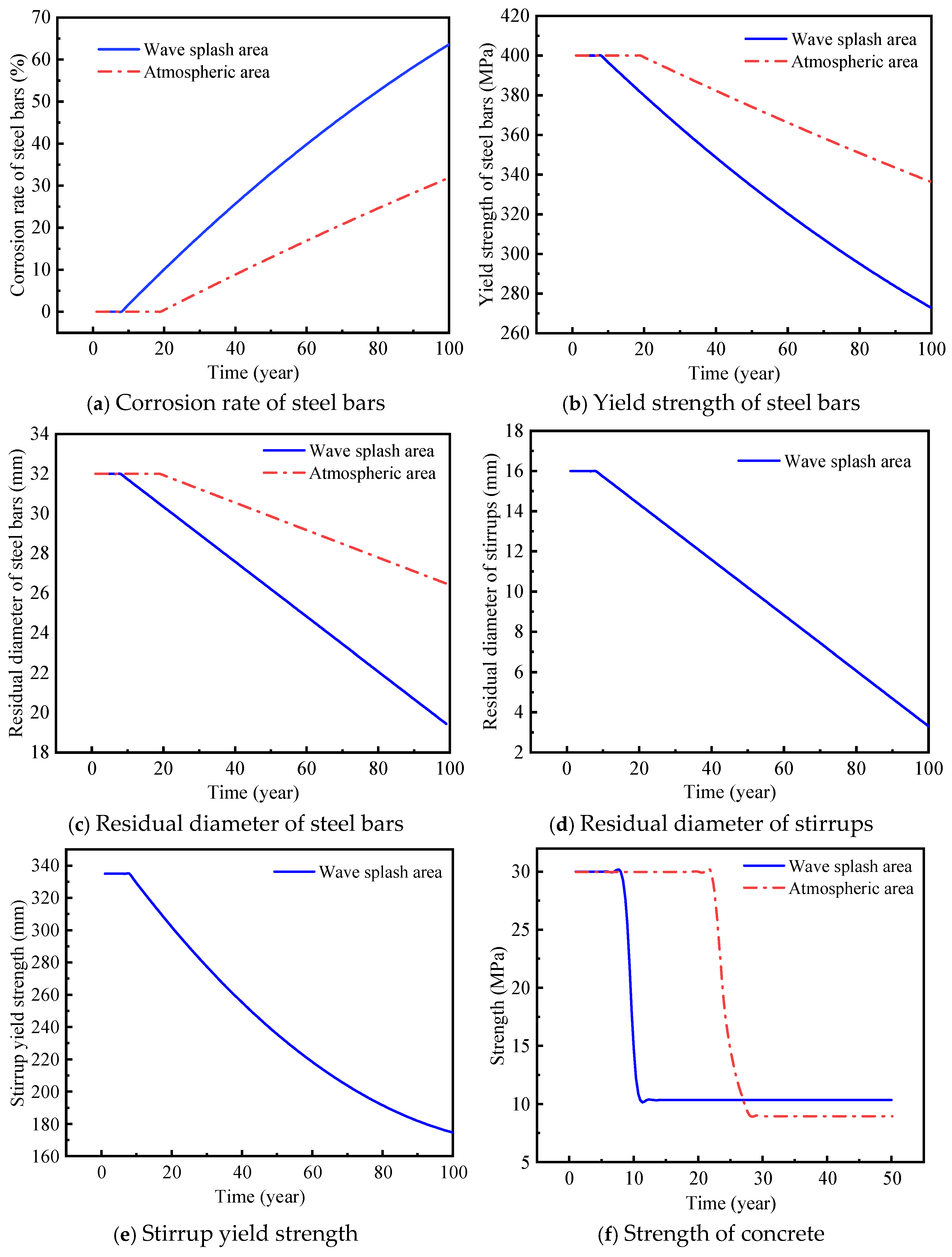
This study reveals that steel bars degrade faster in the wave splash zone, rusting in 8 years compared to 19 years in the atmospheric area. Concrete cracks develop earlier in the splash zone (after 11 years) than in the atmospheric area (28 years). Concrete strength declines earlier in the splash zone, but shows a more significant reduction in the atmospheric area.

(3)

The energy fluctuation period of the high-rise pile cap matches the wave load period. Energy conversion analysis shows that the sum of internal and kinetic energy equals the total energy at all times, confirming the accuracy of the numerical model.

(4)

As the scour depth increases, the transverse displacement of the cap rises, with peak displacement occurring later. Longitudinal displacement occurs earlier on the left of the bridge piles than on the right. Vertical displacement follows a cyclic pattern, with that of left-side piles first increasing and then decreasing, and that of right-side piles decreasing and then increasing. The maximum transverse displacement grows with an increase in corrosion time.

(5)

There is a noticeable concentration of stress at the pile cap connection. As the scour depth increases, the transverse stress in the cap rises. Vertical tensile stress is seen at the pile top, shifting to vertical compressive stress at a depth of 35 m. Both the vertical tensile stress at the top and the compressive stress at 35 m increase with deeper scouring. At a burial depth of between 20 and 60 m, the pile stress first increases and then decreases.

(6)

Wave loads cause abrupt changes in cap acceleration. At a 9 m scour depth, the acceleration peak occurs later than at 3 m. Two main frequency bands, 0–50 Hz and 50–75 Hz, are observed at scour depths of 3 and 9 m, respectively. The maximum acceleration amplitude occurs at the second-order frequency (62 Hz), indicating the importance of the structure’s breaking mode at this frequency.

Although the long-term performance of high-pile caps under the influence of scouring and corrosion has been extensively investigated through comprehensive numerical studies, the modeling and analytical approaches employed in this research still require further validation via experimental testing. Future research should focus on the uncertainty of corrosion and scour rates. In addition, the impact of environmental factors such as temperature variations and pollutants on corrosion and scour should be considered to more accurately predict the long-term performance of high-rise pile cap structures.

References

- Chen, J.; Qu, Y.; Sun, Z. Protection mechanisms, countermeasures, assessments and prospects of local scour for cross-sea bridge foundation: A review. Ocean Eng. 2023, 288, 116145. [Google Scholar] [CrossRef]
- Yang, R.; Li, Y.; Xu, C.; Yang, Y.; Fang, C. Directional effects of correlated wind and waves on the dynamic response of long-span sea-crossing bridges. Appl. Ocean Res. 2023, 132, 103483. [Google Scholar] [CrossRef]
- Shi, X.; Liu, Z.; Guo, T.; Li, W.; Niu, Z.; Ling, F. Research on the Flow-Induced Vibration of Cylindrical Structures Using Lagrangian-Based Dynamic Mode Decomposition. J. Mar. Sci. Eng. 2024, 12, 1378. [Google Scholar] [CrossRef]
- Li, C.Y.; Chi, Y.; Sun, X.Q.; Han, Y.P.; Chen, X.; Zhao, L.C.; Zhang, H. Construction technology of high-rise pile cap foundation of offshore wind power in Taiwan Strait. IOP Conf. Ser. Earth Environ. Sci. 2017, 93, 012037. [Google Scholar] [CrossRef]
- Barnes, I.C.; Frick, K.T.; Deakin, E.; Skabardonis, A. Impact of Peak and Off-Peak Tolls on Traffic in San Francisco–Oakland Bay Bridge Corridor in California. Transp. Res. Rec. 2012, 2297, 73–79. [Google Scholar] [CrossRef]
- Miyata, T.; Yamaguchi, K. Aerodynamics of wind effects on the Akashi Kaikyo Bridge. J. Wind Eng. Ind. Aerodyn. 1993, 48, 287–315. [Google Scholar] [CrossRef]
- Yu, Y.; Li, J.; Li, J.; Xia, Y.; Ding, Z.; Samali, B. Automated damage diagnosis of concrete jack arch beam using optimized deep stacked autoencoders and multi-sensor fusion. Dev. Built Environ. 2023, 14, 100128. [Google Scholar] [CrossRef]
- Yuan, W.; Liu, M. Research on the Wave Load Effect Based on Time History Analysis of Donghai Island Bridge. Adv. Mater. Res. 2014, 919–921, 587–589. [Google Scholar] [CrossRef]
- Ma, X.; Xiong, W.; Fang, Y.; Cai, C.S. Safety assessment of ship-bridge system during sea transportation under complex sea states. Ocean Eng. 2023, 286, 115630. [Google Scholar] [CrossRef]
- Qiu, Z.; Prabhakaran, A.; Su, L.; Zheng, Y. Performance-based seismic resilience and sustainability assessment of coastal RC bridges in aggressive marine environments. Ocean Eng. 2023, 279, 114547. [Google Scholar] [CrossRef]
- Guo, A.; Fang, Q.; Bai, X.; Li, H. Hydrodynamic Experiment of the Wave Force Acting on the Superstructures of Coastal Bridges. J. Bridge Eng. 2015, 20, 04015012. [Google Scholar] [CrossRef]
- Liu, Z.; Shi, X.; Guo, T.; Ren, H.; Zhang, M. Investigation on hydrodynamic response and characteristics of a submerged floating tunnel based on hydrodynamic tests. Ocean Eng. 2024, 300, 117187. [Google Scholar] [CrossRef]
- Yang, Y.; Fahmy, M.F.M.; Guan, S.; Pan, Z.; Zhan, Y.; Zhao, T. Properties and applications of FRP cable on long-span cable-supported bridges: A review. Compos. Part B Eng. 2020, 190, 107934. [Google Scholar] [CrossRef]
- Meier, U. Proposal for a Carbon Fibre Reinforced Composite Bridge across the Strait of Gibraltar at its Narrowest Site. Proc. Inst. Mech. Eng. Part B Manag. Eng. Manuf. 1987, 201, 73–78. [Google Scholar] [CrossRef]
- Wang, Q.; Li, L.; Zhao, Y.; Song, Y.; Zhang, C. Feasibility assessment and application of sea sand in concrete production: A review. Structures 2024, 60, 105891. [Google Scholar] [CrossRef]
- Alraeeini, A.S.; Nikbakht, E. Corrosion effect on the flexural behaviour of concrete filled steel tubulars with single and double skins using engineered cementitious composite. Structures 2022, 44, 1680–1694. [Google Scholar] [CrossRef]
- Bazli, M.; Dorothea Luck, J.; Rajabipour, A.; Arashpour, M. Bond-slip performance of seawater sea sand concrete filled filament wound FRP tubes under cyclic and static loads. Structures 2023, 52, 889–903. [Google Scholar] [CrossRef]
- Yuan, Y.; Jiang, J.; Peng, T. Corrosion Process of Steel Bar in Concrete in Full Lifetime. ACI Mater. J. 2010, 107, 562–567. [Google Scholar]
- Ou, Y.-C.; Tsai, L.-L.; Chen, H.-H. Cyclic performance of large-scale corroded reinforced concrete beams. Earthq. Eng. Struct. Dyn. 2012, 41, 593–604. [Google Scholar] [CrossRef]
- Akiyama, M.; Frangopol, D.M. Long-term seismic performance of RC structures in an aggressive environment: Emphasis on bridge piers. Struct. Infrastruct. Eng. 2014, 10, 865–879. [Google Scholar] [CrossRef]
- Fan, W.; Sun, Y.; Sun, W.; Huang, X.; Liu, B. Effects of Corrosion and Scouring on Barge Impact Fragility of Bridge Structures Considering Nonlinear Soil–Pile Interaction. J. Bridge Eng. 2021, 26, 04021058. [Google Scholar] [CrossRef]
- Liu, Z.; Niu, S.; Qian, J.; Guo, T. Investigation on flooding dynamic response and mitigation measure of river bridge. Eng. Fail. Anal. 2025, 167, 108987. [Google Scholar] [CrossRef]
- Niu, S.; Liu, Z.; Guo, T.; Guo, A.; Liu, A. Dynamic characteristics and force analysis of box girder under tsunami action based on level-set method. Struct. Infrastruct. Eng. 2025, 1–22. [Google Scholar] [CrossRef]
- Geng, B.; Sun, K.; Gao, P.; Jin, R.; Jiang, S. Experimental and Numerical Investigations for Impact Loading on Platform Decks. J. Mar. Sci. Eng. 2024, 12, 899. [Google Scholar] [CrossRef]
- Albalawi, W.; Taha, H.H.; El-Sapa, S. Effect of the permeability on the interaction between two spheres oscillating through Stokes-Brinkmann medium. Heliyon 2023, 9, e14396. [Google Scholar] [CrossRef] [PubMed]
- Xu, B.; Wei, K. Numerical simulation of wave forces on elevated pile cap of sea-crossing bridges based on RANS. Railw. Stand. Des. 2019, 63, 6. [Google Scholar]
- Deng, L.; Yang, W.; Li, Q.; Li, A. CFD investigation of the cap effects on wave loads on piles for the pile-cap foundation. Ocean Eng. 2019, 183, 249–261. [Google Scholar] [CrossRef]
- Al-Hanaya, A.; El–Sapa, S. Impact of permeability and fluid parameters in couple stress media on rotating eccentric spheres. Open Phys. 2024, 22, 20240112. [Google Scholar] [CrossRef]
- Hirt, C.W.; Nichols, B.D. Volume of fluid (VOF) method for the dynamics of free boundaries. J. Comput. Phys. 1981, 39, 201–225. [Google Scholar] [CrossRef]
- Ye, X.; Zhou, X.; Wang, M.; Qiao, D.; Zhao, X.; Wang, L. Global Responses Analysis of Submerged Floating Tunnel Considering Hydroelasticity Effects. J. Mar. Sci. Eng. 2024, 12, 1854. [Google Scholar] [CrossRef]
- Algatheem, A.M.; Taha, H.H.; El-Sapa, S. Interaction Between Two Rigid Hydrophobic Spheres Oscillating in an Infinite Brinkman–Stokes Fluid. Mathematics 2025, 13, 218. [Google Scholar] [CrossRef]
- Weller, H.G.; Tabor, G.; Jasak, H.; Fureby, C. A tensorial approach to computational continuum mechanics using object-oriented techniques. Comput. Phys. 1998, 12, 620–631. [Google Scholar] [CrossRef]
- Ducrozet, G.; Bouscasse, B.; Gouin, M.; Ferrant, P.; Bonnefoy, F. CN-Stream: Open-source library for nonlinear regular waves using stream function theory. arXiv 2019, arXiv:1901.10577v1. [Google Scholar]
- Karadeniz, H. Wave-Current and Fluid-Structure Interaction Effects on the Stochastic Analysis of Offshore Structures. In Proceedings of the Second International Offshore and Polar Engineering Conference, San Francisco, CA, USA, 14–19 June 1992. [Google Scholar]
- Fan, W.; Sun, Y.; Yang, C.; Sun, W.; He, Y. Assessing the response and fragility of concrete bridges under multi-hazard effect of vessel impact and corrosion. Eng. Struct. 2020, 225, 111279. [Google Scholar] [CrossRef]
- Third Harbor Engineering Investigation and Design Institute of the Ministry of Transport. Code for Pile Foundation in Port Engineering; People’s Transportation Publishing House: Beijing, China, 2012. [Google Scholar]
- DNV-OS-J101; Design of Offshore Wind Turbine Structures. Det Norske Veritas: Bærum, Norway, 2010.
- American Petroleum Institute (API). Petroleum and Natural Gas Industries-Specific Requirements for Offshore Structures. Part 4-Geotechnical and Foundation Design Considerations. 2011. Available online: http://refhub.elsevier.com/S0267-7261(19)30591-3/sref25 (accessed on 15 February 2025).
- Boulanger, R.; Curras, C.; Kutter, B.; Wilson, D.; Abghari, A. Seismic Soil-Pile-Structure Interaction Experiments and Analyses. J. Geotech. Geoenviron. Eng. 1999, 125, 750–759. [Google Scholar] [CrossRef]
- Guo, X.; Zhang, C.; Chen, Z. Nonlinear Dynamic Response and Assessment of Bridges under Barge Impact with Scour Depth Effects. J. Perform. Constr. Facil. 2020, 34, 04020058. [Google Scholar] [CrossRef]
- Imam, B. Chapter Six—Climate Change Impact for Bridges Subjected to Scour and Corrosion. In Climate Adaptation Engineering; Bastidas-Arteaga, E., Stewar, M.G., Eds.; Butterworth-Heinemann: Oxford, UK, 2019; pp. 165–206. [Google Scholar]
- Calvi, G.M.; Priestley, M.J.N.; Kowalsky, M.J. Displacement-Based Seismic Design of Bridges. Struct. Eng. Int. 2013, 23, 112–121. [Google Scholar] [CrossRef]
- Guo, A.; Yuan, W.; Lan, C.; Guan, X.; Li, H. Time-dependent seismic demand and fragility of deteriorating bridges for their residual service life. Bull. Earthq. Eng. 2015, 13, 2389–2409. [Google Scholar] [CrossRef]
- Balafas, K.; Kiremidjian, A.S. Reliability assessment of the rotation algorithm for earthquake damage estimation. Struct. Infrastruct. Eng. 2015, 11, 51–62. [Google Scholar] [CrossRef]
- Liang, Z.; Lee, G.C. Towards establishing practical multi-hazard bridge design limit states. Earthq. Eng. Eng. Vib. 2013, 12, 333–340. [Google Scholar] [CrossRef]
- Khan, R.; Datta, T. Effect of Support Flexibility and Soil- Structure Interaction on Seismic Risk Analysis of Harp Type Cable Stayed Bridges. Ing. Sismica 2014, 31, 32–46. [Google Scholar]
- Cairns, J.; Plizzari, G.; Du, Y.; Law, D.; Franzoni, C. Mechanical properties of corrosion-damaged reinforcement. ACI Mater. J. 2005, 102, 256–264. [Google Scholar]
- Du, Y.G.; Clark, L.A.; Chan, A.H.C. Residual capacity of corroded reinforcing bars. Mag. Concr. Res. 2005, 57, 135–147. [Google Scholar] [CrossRef]
- Molina, F.J.; Alonso, C.; Andrade, C. Cover cracking as a function of rebar corrosion: Part 2—Numerical model. Mater. Struct. 1993, 26, 532–548. [Google Scholar] [CrossRef]
- Vecchio, F.J.; Collins, M.P. The Modified Compression-Field Theory for Reinforced Concrete Elements Subjected to Shear. ACI Struct. J. 1986, 83, 219–231. [Google Scholar]
- Biondini, F.; Vergani, M. Damage modeling and nonlinear analysis of concrete bridges under corrosion. In Proceedings of the Sixth International Conference of Bridge Maintenance, Safety and Management (IABMAS 2012), Stresa, Italy, 8–12 July 2012; pp. 949–957. [Google Scholar]
- Coronelli, D.; Gambarova, P. Structural Assessment of Corroded Reinforced Concrete Beams: Modeling Guidelines. J. Struct. Eng. 2004, 130, 1214–1224. [Google Scholar] [CrossRef]
- Vidal, T.; Castel, A.; François, R. Analyzing crack width to predict corrosion in reinforced concrete. Cem. Concr. Res. 2004, 34, 165–174. [Google Scholar] [CrossRef]
- Zheng, Y.; Chen, B.; Chen, W. Evaluation of the seismic responses of a long-span cable-stayed bridge located in complex terrain based on an SHM-oriented model. Stahlbau 2015, 84, 252–266. [Google Scholar] [CrossRef]
- Johnson, P.A.; Dock, D.A. Probabilistic Bridge Scour Estimates. J. Hydraul. Eng. 1998, 124, 750–754. [Google Scholar] [CrossRef]
- Xu, B.; Wei, K.; Qin, S.; Hong, J. Experimental study of wave loads on elevated pile cap of pile group foundation for sea-crossing bridges. Ocean Eng. 2020, 197, 106896. [Google Scholar] [CrossRef]