
Marine Gravity Field Modeling Using SWOT Altimetry Data in South China Sea

Abstract
1. Introduction
2. Study Area and Dataset
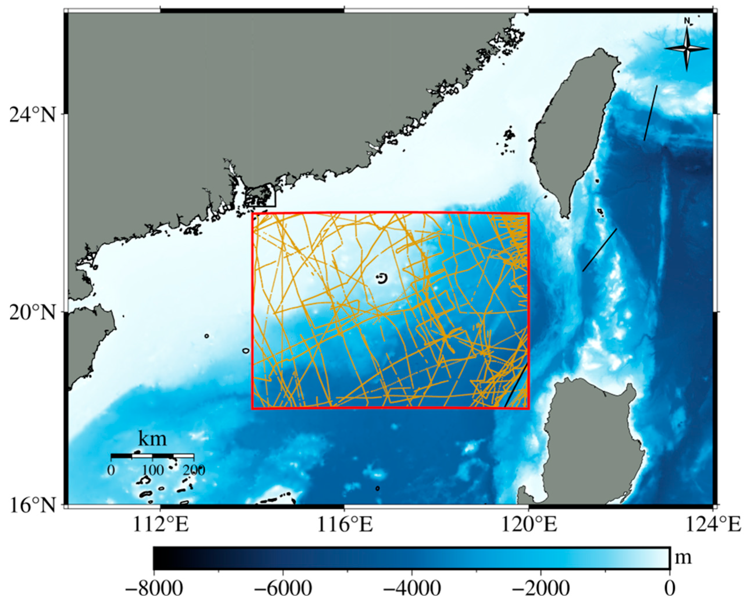
2.1. Study Area
2.2. Dataset in Study Area
2.2.1. Shipborne Gravity Data
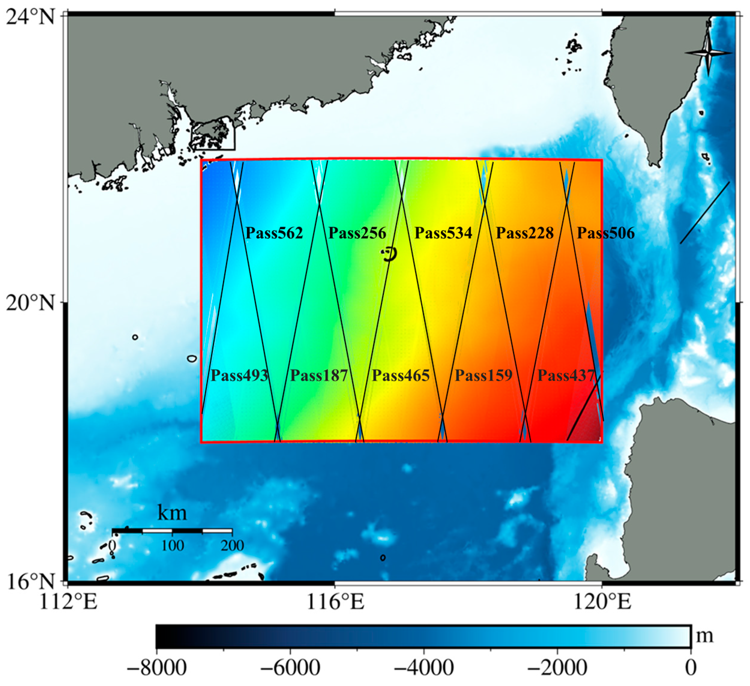
2.2.2. SWOT Altimetry Data
- ancillary_surface_classification_flag = 0. Only ocean data were selected;
- distance_to_coast > 2000 m. Nearshore altimetry data are susceptible to influences such as topography, sea state variations, and abnormal radar echo patterns, which can degrade the measurement accuracy. Therefore, data within 2000 m of the coastline were excluded to minimize the impact of coastal interference on the calculations;
- Significant Wave Height (SWH) < 6 m. Under high sea state conditions (SWH > 6 m), the quality of altimetry data can be significantly compromised, leading to increased measurement errors. Thus, data with an SWH greater than 6 m were filtered out to reduce the uncertainties caused by intense sea state variations [26];
- ssha_karin_qual = 0. This flag serves as a critical filtering parameter to effectively exclude poor-quality data from the wide swath edges and center, ensuring the overall quality and reliability of the altimetry data.
2.2.3. SIO Model
2.2.4. Mean Sea Surface Model
2.2.5. Mean Dynamic Topography Model
3. Method
3.1. Calculation DOV Based on Eight-Directional Geoid Gradient
3.2. Inverse Vening–Meinesz (IVM) Method
4. Results and Analysis
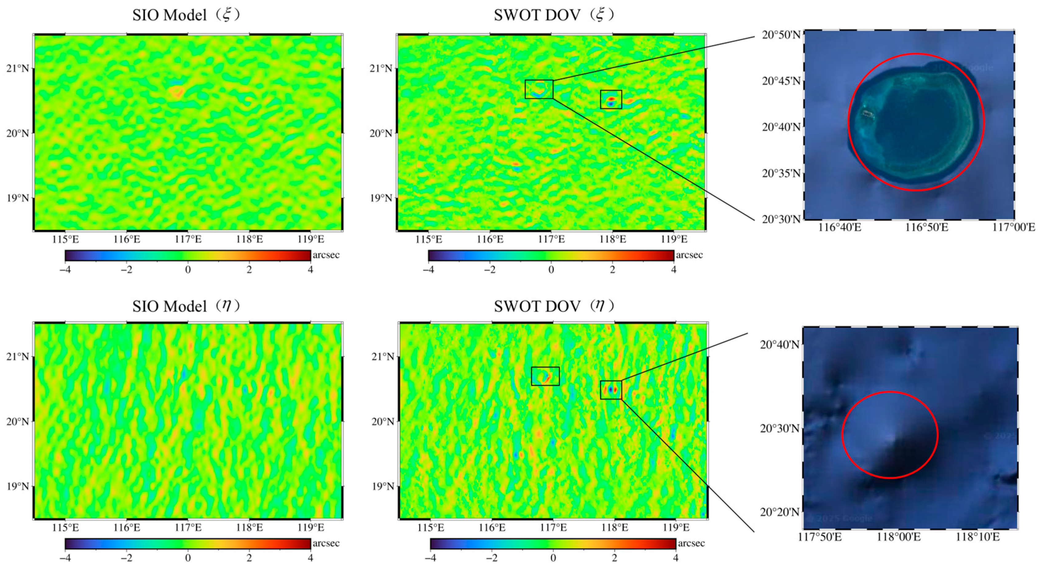
4.1. Results of the SWOT DOV Calculation
4.2. Impact on the Accuracy of IVM Method Using SWOT DOV
5. Discussion
6. Conclusions
- (1)
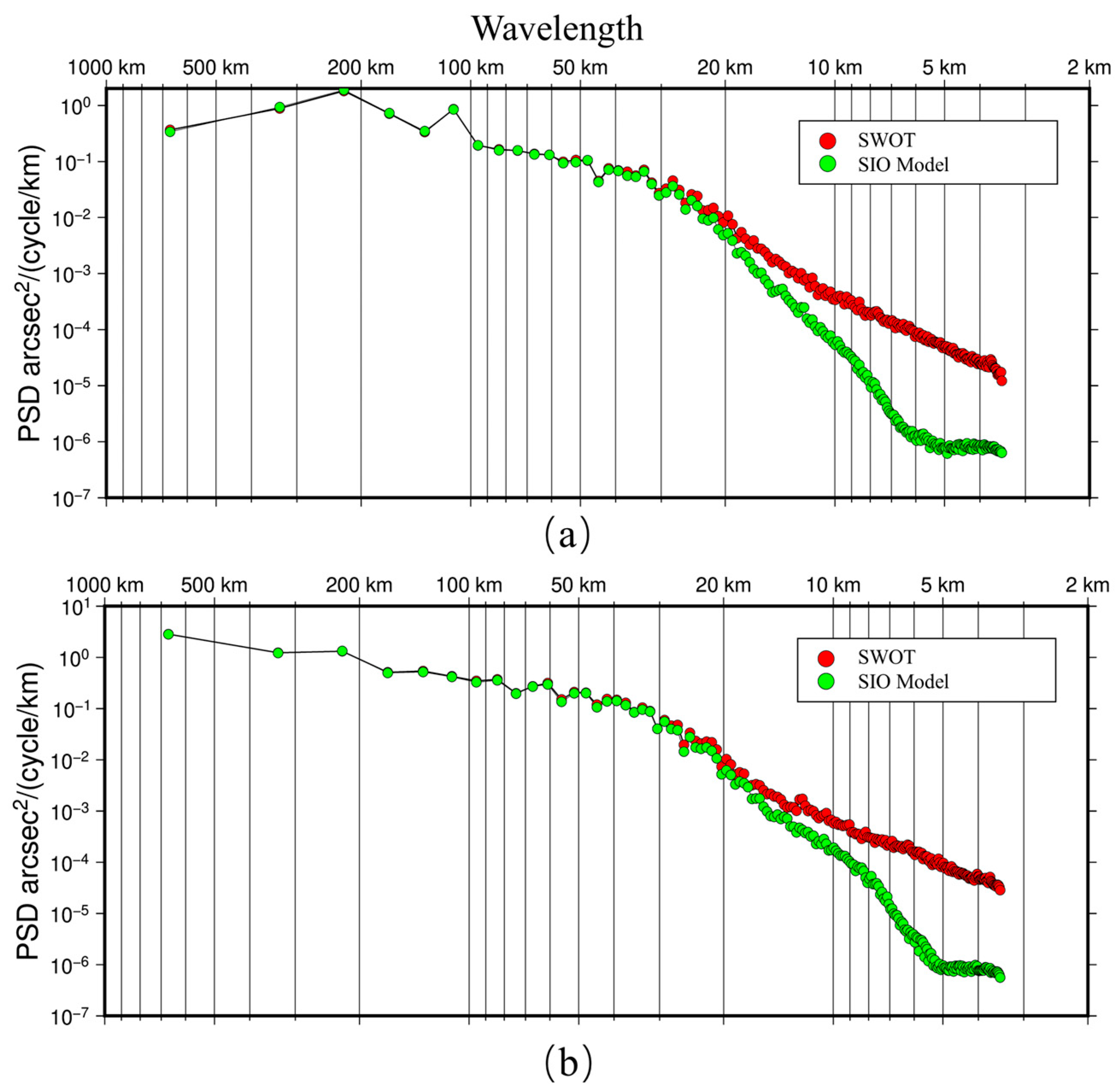
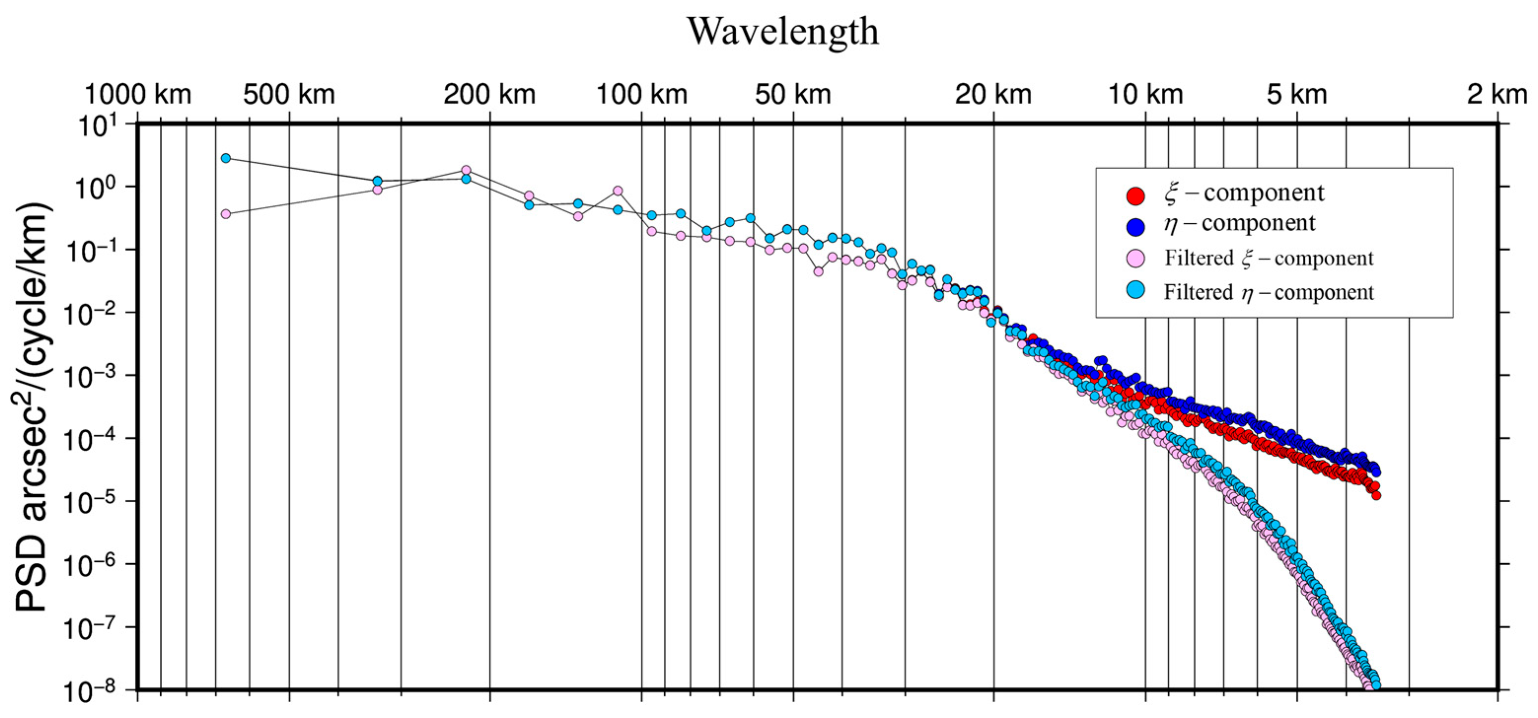
- The DOVs derived from SWOT data can precisely characterize seafloor topographic features. Compared with shipborne gravity data, the differences between the η and ξ components of DOVs derived from nearly one year of SWOT data are significantly smaller than those from traditional altimetry satellites. The accuracy of these components is comparable to the multi-source altimetry fusion model SIO_v32.1. PSD analysis indicates that, compared to the SIO model, SWOT shows spectral gains primarily in the short-wavelength range of 3.5–20 km, demonstrating that SWOT’s wide-swath interferometric mode effectively captures medium to small-scale sea surface height signals;
- (2)
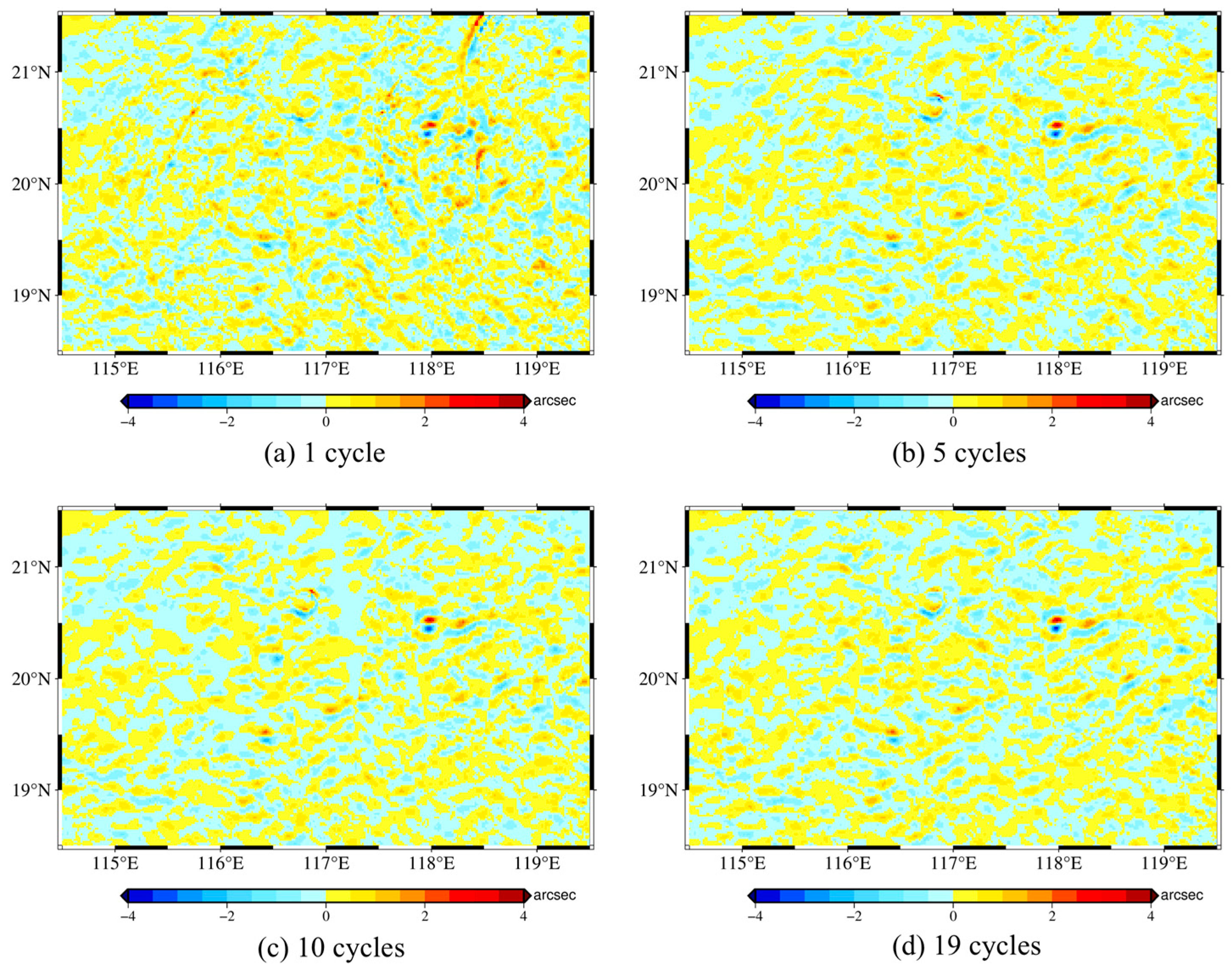
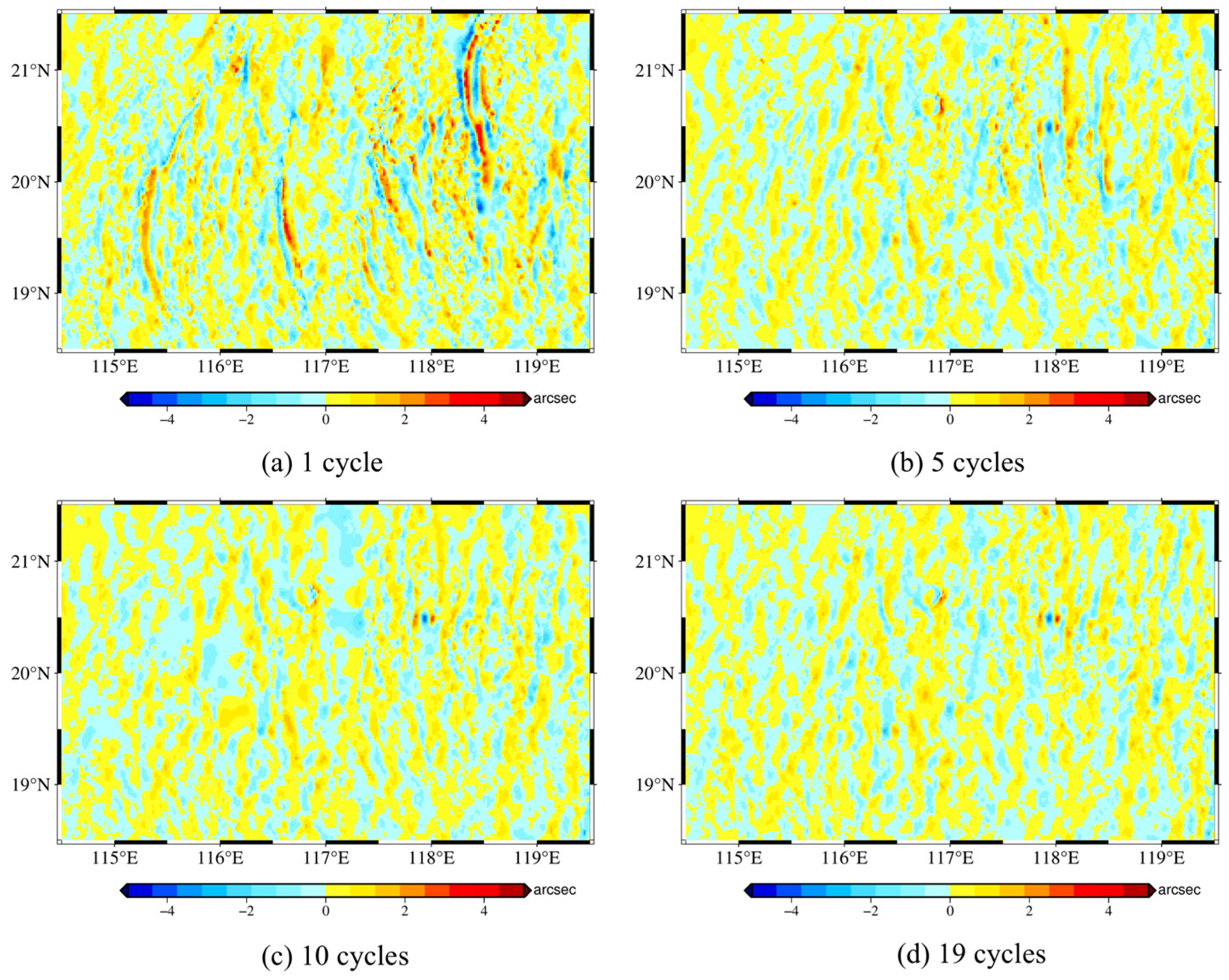
- Increasing the SWOT observation period improves the accuracy of DOVs, but the efficiency of the improvement varies directionally. Specifically, the ξ component reaches a stable and satisfactory accuracy with fewer observation cycles, whereas the η component requires the accumulation of more observation cycles to achieve a comparable accuracy. This directional difference indicates that cross-track errors caused by factors such as baseline roll and phase drift are critical limitations affecting the accuracy of the η component. Although the impact of these errors can be partially mitigated by an increasing data accumulation, they cannot be completely eliminated, suggesting the necessity for developing targeted correction algorithms;
- (3)
- The SWOT DOV gains are mainly concentrated within the 3.5–20 km wavelength band, but high-frequency signals in this band are prone to amplification by noise during the inversion of gravity anomalies using the IVM method. Through an analysis involving four filtering experiments, it is found that applying a 10 km Gaussian low-pass filter to DOV components improves the gravity anomaly inversion accuracy, with noise in the η component having a more pronounced impact. Further PSD analysis confirms that within this band, the interference from noise surpasses the actual DOV signals, particularly in the η component.
Author Contributions
Funding
Data Availability Statement
Acknowledgments
Conflicts of Interest
References
- Flechtner, F.; Reigber, C.; Rummel, R.; Balmino, G. Satellite Gravimetry: A Review of Its Realization. Surv. Geophys. 2021, 42, 1029–1074. [Google Scholar] [CrossRef] [PubMed]
- Zhang, S.; Andersen, O.B.; Kong, X.; Li, H. Inversion and Validation of Improved Marine Gravity Field Recovery in South China Sea by Incorporating HY-2A Altimeter Waveform Data. Remote Sens. 2020, 12, 802. [Google Scholar] [CrossRef]
- Sandwell, D.; Garcia, E.; Soofi, K.; Wessel, P.; Chandler, M.; Smith, W.H.F. Toward 1-MGal Accuracy in Global Marine Gravity from CryoSat-2, Envisat, and Jason-1. Lead. Edge 2013, 32, 892–899. [Google Scholar] [CrossRef]
- Yu, D.; Hwang, C.; Andersen, O.B.; Chang, E.T.Y.; Gaultier, L. Gravity Recovery from SWOT Altimetry Using Geoid Height and Geoid Gradient. Remote Sens. Environ. 2021, 265, 112650. [Google Scholar] [CrossRef]
- Sandwell, D.T.; Smith, W.H.F. Marine Gravity Anomaly from Geosat and ERS 1 Satellite Altimetry. J. Geophys. Res. Solid Earth 1997, 102, 10039–10054. [Google Scholar] [CrossRef]
- Hwang, C.; Kao, E.C.; Parsons, B. Global Derivation of Marine Gravity Anomalies from Seasat, Geosat, ERS-1 and TOPEX/Poseidon Altimeter Data. Geophys. J. Int. 1998, 134, 449–459. [Google Scholar] [CrossRef]
- Haxby, W.F.; Karner, G.D.; LaBrecque, J.L.; Weissel, J.K. Digital Images of Combined Oceanic and Continental Data Sets and Their Use in Tectonic Studies. Eos Trans. Am. Geophys. Union 1983, 64, 995–1004. [Google Scholar] [CrossRef]
- Wang, Y.M. On the Ellipsoidal Corrections to Gravity Anomalies Computed Using the Inverse Stokes Integral. J. Geod. 1999, 73, 29–34. [Google Scholar] [CrossRef]
- Andersen, O.B.; Knudsen, P. Global Marine Gravity Field from the ERS-1 and Geosat Geodetic Mission Altimetry. J. Geophys. Res. Ocean. 1998, 103, 8129–8137. [Google Scholar] [CrossRef]
- Hwang, C. Inverse Vening Meinesz Formula and Deflection-Geoid Formula: Applications to the Predictions of Gravity and Geoid over the South China Sea. J. Geod. 1998, 72, 304–312. [Google Scholar] [CrossRef]
- Hwang, C.; Hsu, H.Y.; Jang, R.J. Global Mean Sea Surface and Marine Gravity Anomaly from Multi-Satellite Altimetry: Applications of Deflection-Geoid and Inverse Vening Meinesz Formulae. J. Geod. 2002, 76, 407–418. [Google Scholar] [CrossRef]
- Sandwell, D.T.; Smith, W.H.F. Global Marine Gravity from Retracked Geosat and ERS-1 Altimetry: Ridge Segmentation versus Spreading Rate. J. Geophys. Res. Solid Earth 2009, 114, B01411. [Google Scholar] [CrossRef]
- Hwang, C.; Parsons, B. An Optimal Procedure for Deriving Marine Gravity from Multi-Satellite Altimetry. Geophys. J. Int. 1996, 125, 705–718. [Google Scholar] [CrossRef]
- Le Traon, P.Y.; Ogor, F. ERS-1/2 Orbit Improvement Using TOPEX/POSEIDON: The 2 Cm Challenge. J. Geophys. Res. Ocean. 1998, 103, 8045–8057. [Google Scholar] [CrossRef]
- Sandwell, D.T.; Harper, H.; Tozer, B.; Smith, W.H.F. Gravity Field Recovery from Geodetic Altimeter Missions. Adv. Space Res. 2021, 68, 1059–1072. [Google Scholar] [CrossRef]
- Andersen, O.B.; Knudsen, P.; Berry, P.A.M. The DNSC08GRA Global Marine Gravity Field from Double Retracked Satellite Altimetry. J. Geod. 2010, 84, 191–199. [Google Scholar] [CrossRef]
- Yu, Y.; Sandwell, D.T.; Gille, S.T.; Villas Bôas, A.B. Assessment of ICESat-2 for the Recovery of Ocean Topography. Geophys. J. Int. 2021, 226, 456–467. [Google Scholar] [CrossRef]
- Andersen, O.B.; Knudsen, P. The DTU17 Global Marine Gravity Field: First Validation Results. In Proceedings of the International Association of Geodesy Symposia, Chania, Greece, 23–26 April 2018; Volume 150, pp. 83–87. [Google Scholar]
- Hwang, C.; Yu, D. Transforming Coastal Mapping from Space. Science 2024, 386, 1222–1223. [Google Scholar] [CrossRef]
- Ma, G.; Jin, T.; Jiang, P.; Shi, J.; Zhou, M. Calibration of the Instrumental Errors on Marine Gravity Recovery from SWOT Altimeter. Mar. Geod. 2023, 46, 496–522. [Google Scholar] [CrossRef]
- Wan, X.; Wang, F.; Guo, H.; Liu, B. Impact of Errors in Environmental Correction on Gravity Field Recovery Using Interferometric Radar Altimeter Observations. Remote Sens. 2022, 14, 6299. [Google Scholar] [CrossRef]
- Wang, J.; Xu, Y.; Zhang, Q.; Wang, Y.; Zhu, C.; Xu, H.; Zhang, L. Improving High-Frequency Marine Gravity Anomaly Recovery: The Efficacy of SWOT Wide-Swath Altimetry. IEEE Geosci. Remote Sens. Lett. 2024, 21, 7505905. [Google Scholar] [CrossRef]
- Wessel, P.; Watts, A.B. On the Accuracy of Marine Gravity Measurements. J. Geophys. Res. 1988, 93, 393–413. [Google Scholar] [CrossRef]
- Smith, R.T. Calculus Early Transcendentals Functions; McGraw-Hill Higher Education: New York, NY, USA, 2007; p. 53. [Google Scholar]
- Zingerle, P.; Pail, R.; Gruber, T.; Oikonomidou, X. The combined global gravity field model XGM2019e. J. Geod. 2020, 94, 66. [Google Scholar] [CrossRef]
- Yu, Y.; Sandwell, D.T.; Dibarboure, G.; Chen, C.; Wang, J. Accuracy and Resolution of SWOT Altimetry: Foundation Seamounts. Earth Space Sci. 2024, 11, e2024EA003581. [Google Scholar] [CrossRef]
- Schaeffer, P.; Pujol, M.I.; Veillard, P.; Faugere, Y.; Dagneaux, Q.; Dibarboure, G.; Picot, N. The CNES CLS 2022 Mean Sea Surface: Short Wavelength Improvements from CryoSat-2 and SARAL/AltiKa High-Sampled Altimeter Data. Remote Sens. 2023, 15, 2910. [Google Scholar] [CrossRef]
- Jousset, S.; Mulet, S.; Greiner, E.; Wilkin, J.; Vidar, L.; Chafik, L.; Raj, R.; Bonaduce, A.; Picot, N.; Dibarboure, G. New Global Mean Dynamic Topography CNES-CLS-22 Combining Drifters, Hydrological Profiles and High Frequency Radar Data. Authorea Preprints. 2025. Available online: https://essopenarchive.org/users/704094/articles/689640-new-global-mean-dynamic-topography-cnes-cls-22-combining-drifters-hydrography-profiles-and-high-frequency-radar-data (accessed on 1 March 2025).
- Cooley, J.W.; Tukey, J.W. An Algorithm for the Machine Calculation of Complex Fourier Series. Math. Comput. 1965, 19, 297–301. [Google Scholar] [CrossRef]


| Shipborne Gravity Anomaly | Min | Max | Mean | STD |
|---|---|---|---|---|
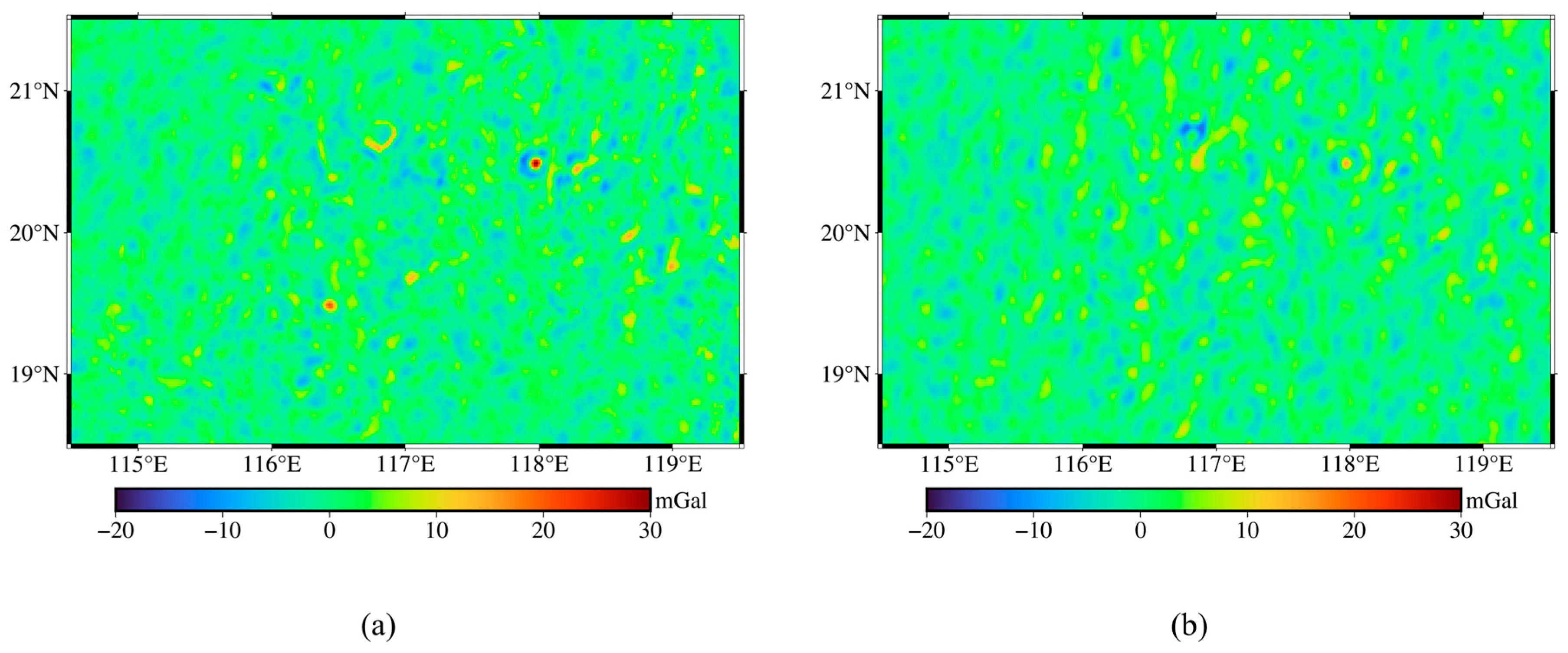
| Before correction | −25.72 | 26.88 | 2.77 | 8.83 |
| After correction | −20.43 | 23.51 | 0.00 | 4.90 |
| Model | DOV | Max | Min | Mean | RMS | STD |
|---|---|---|---|---|---|---|
| SWOT | 2.94 | −3.56 | 0.04 | 0.77 | 0.77 | |
| 3.75 | −4.09 | −0.01 | 0.86 | 0.86 | ||
| SIO | 2.96 | −3.54 | 0.07 | 0.76 | 0.76 | |
| 3.66 | −4.34 | −0.02 | 0.87 | 0.87 |
| Group | Max | Min | Mean | STD |
|---|---|---|---|---|
| Group 1 | 23.99 | −23.66 | 0.65 | 4.97 |
| Group 2 | 23.45 | −23.40 | 0.65 | 4.95 |
| Group 3 | 23.77 | −23.22 | 0.65 | 4.92 |
| Group 4 | 23.23 | −22.95 | 0.66 | 4.90 |
| Period | DOV | Max | Min | Mean | STD |
|---|---|---|---|---|---|
| 1 cycle | 9.00 | −8.98 | −0.04 | 0.83 | |
| 4.56 | −4.57 | −0.01 | 1.07 | ||
| 5 cycles | 8.86 | −8.73 | −0.02 | 0.77 | |
| 3.84 | −4.18 | −0.02 | 0.91 | ||
| 10 cycles | 9.03 | −9.31 | −0.02 | 0.77 | |
| 3.92 | −4.03 | −0.01 | 0.89 | ||
| 19 cycles | 8.80 | −8.82 | −0.02 | 0.77 | |
| 3.75 | −4.09 | −0.01 | 0.86 |
Disclaimer/Publisher’s Note: The statements, opinions and data contained in all publications are solely those of the individual author(s) and contributor(s) and not of MDPI and/or the editor(s). MDPI and/or the editor(s) disclaim responsibility for any injury to people or property resulting from any ideas, methods, instructions or products referred to in the content. |
© 2025 by the authors. Licensee MDPI, Basel, Switzerland. This article is an open access article distributed under the terms and conditions of the Creative Commons Attribution (CC BY) license (https://creativecommons.org/licenses/by/4.0/).
Share and Cite
Tu, Z.; Jiang, T.; Zhao, F. Marine Gravity Field Modeling Using SWOT Altimetry Data in South China Sea. J. Mar. Sci. Eng. 2025, 13, 827. https://doi.org/10.3390/jmse13050827
Tu Z, Jiang T, Zhao F. Marine Gravity Field Modeling Using SWOT Altimetry Data in South China Sea. Journal of Marine Science and Engineering. 2025; 13(5):827. https://doi.org/10.3390/jmse13050827
Chicago/Turabian StyleTu, Zejie, Tao Jiang, and Fuxi Zhao. 2025. "Marine Gravity Field Modeling Using SWOT Altimetry Data in South China Sea" Journal of Marine Science and Engineering 13, no. 5: 827. https://doi.org/10.3390/jmse13050827
APA StyleTu, Z., Jiang, T., & Zhao, F. (2025). Marine Gravity Field Modeling Using SWOT Altimetry Data in South China Sea. Journal of Marine Science and Engineering, 13(5), 827. https://doi.org/10.3390/jmse13050827