Numerical Study on the Influence of Rudder Fillets on Submarine Wake Field and Noise Characteristics

Abstract

The submarine rudder configuration and arrangement significantly impact its hydrodynamic performance. This paper takes the SUBOFF standard submarine model as the research object, constructs a geometrically parameterized rudder fillet structure based on parabolic parametric equations, and adopts the improved delayed separation vortex (IDDES) turbulence model to carry out numerical simulation research on the submarine rounding flow field with crossed and “X” rudder configurations. By comparing and analyzing the effects of different fillet parameters and rudder layouts on the generation mechanism of the horseshoe vortex, vortex system strength characteristics, and the distribution of the wake companion flow field at the velocity of 7.161 m/s, it is found that the introduction of the rudder fillet structure can effectively destabilize the horseshoe vortex and significantly reduce the axial velocity inhomogeneity of propeller plane. In addition, the improvement effect of the flow field in the near-axis region (r/R ∈ (0, 0.5)) is particularly significant. Compared with the crossed rudder, the “X” layout shows better flow control performance, with the maximum reduction in the axial relative velocity of the propeller plane surface reaching 49.34%, which is 24.25% higher than that of the SUBOFF baseline model, and the addition of two distributions of rudder fillets can reduce the hydrodynamic noise of the submarine by 4.6 dB vs. 5.6 dB at most. The results provide an essential hydrodynamic basis for optimizing the submarine rudder system.

1. Introduction

As one of the two most common submarine attachments, the rudder can control a submarine’s heading and improve a submarine’s maneuverability. The rudder is generally composed of four rudder blades, and the number of rudder blades determines the diversity of the rudder distribution. The standard rudder blade is mostly a crossed distribution; there are also X-type multi-angle distributions, T-type distributions, and so on. Among them, an X-shaped rudder is a more common rudder configuration than a crossed rudder, and Xiao et al. [1] reduced the area of an X rudder to achieve better wake quality. Zhou et al. [2] concluded that the X rudder has the advantages of good maneuverability, not exceeding the width in the lateral direction and not exceeding the baseline in the vertical direction. Cao et al. [3] designed an X-rudder submarine to generate a larger restoring moment when the sailing direction changes, increasing its heading stability. Jiao Yu et al. [4] investigated the X-rudder submarine with a multi-angle distribution. They found that the 45°X-rudder submarine aft pressure length is more uniform, and the resistance is minimized when sailing. It can be seen that the rudder has a pivotal role in submarines.

As shown in Figure 1, when the fluid movement encounters an obstacle, the flow velocity decreases, generating a larger downstream pressure and a smaller upstream pressure, forming a counter-pressure gradient. When the counter-pressure gradient is significant to a certain extent, the original movement of the fluid will not only stop but also under the action of the counter-pressure gradient against the flow (in the opposite direction) in the wall close to the root of the obstacle, close to the wall of the corner area, the formation of the downstream flow of the upward roll along the root area of the obstacle. The horseshoe-like vortex structure is the formation mechanism and source of the horseshoe vortex. It mainly consists of a pair of symmetrical vortices, extending downstream around the sides of the blunt body, forming a “U” shaped structure. The high vortex area of the horseshoe vortex is concentrated in the leading edge and both sides of the blunt body, accompanied by strong secondary flow and boundary layer separation. Through the turbulent energy dissipation and pressure pulsation, it significantly affects the drag, lift, and surface pressure distribution of the blunt body. During submarine navigation, there is hydrodynamic interference between the submarine’s appendage and the main body, and horseshoe vortices are generated when the fluid flows through. When the fluid encounters the rudder, it will generate a great counterpressure gradient at its leading edge, and the flow field undergoes obvious flow separation and generates strong vortex flows. The formation of these vortices will drive the surrounding flow field to form a vortex tube extending towards the transom. Due to the streamlined structure of the submarine’s transom, these vortex tubes will further propagate downstream to converge into wake vortices, leading to the unevenness of the submarine’s propeller plane companion flow, which is a key factor affecting the submarine’s vibration and noise during operation. Thus, the horseshoe vortex generated by the submarine’s sail and rudder is an important cause of the unevenness of the propeller plane companion flow.

The horseshoe vortex has high strength and weak dissipation. When the vortex propagates to the transom, the wake becomes a complex flow area characterized by turbulence pulsation, the viscous effect, and vortex motion, resulting in a serious inhomogeneity in the wake flow field, which will inevitably lead to an increase in the submarine surface pulsation pressure and hydrodynamic noise, which affects the stealthy performance of the submarine.

The horseshoe vortex is the primary noise source of the attached body, so the shape optimization of the attached body plays an essential role in suppressing the horseshoe vortex. The shape optimization of the fillet is primarily used in the enclosure and rudder, improving the homogeneity in the companion flow field of the submarine’s wake and reducing the horseshoe vortex to lower the noise. In the study of the enclosure, Toxopeus et al. [5] found that adding a fillet not only suppressed the strength of horseshoe vortices at the enclosure but also improved the circumferential homogeneity in the incoming flow at the propeller plane and the quality of the submarine wake. Yeo et al. [6] added convex and concave fillets at the leading and trailing edges of the enclosure and rudder, which reduced the backpressure gradient around the appendage and the total noise by up to 20 dB. Mohsen Rahmani et al. [7] compared a prototype and a leading-edge corner-filling-type enclosure. They found that the vortex power around the latter was significantly reduced compared to the former, and the vortex intensity was reduced by up to 18%. Wang et al. [8] investigated the inhibition effect of different leading-edge fillets on the horseshoe vortex. They found that parabolic corner filling had an inhibition effect on the intensity of the horseshoe vortex and the hydrodynamic noise, and the noise could be reduced by up to 4.69 dB. Li et al. [9] added a linear filler angle to a submarine rudder to improve the uniformity of the propeller companion flow field and reduce the submarine radiated noise. Jin et al. [10] investigated three different filler angle structures, including concave, convex, and linear rudders. The results showed that the three structures reduced the circumferential inhomogeneity in the incoming flow from the propeller, effectively improving the propeller plane flow quality. Dai et al. [11] found that installing rudder fillets helped reduce the turbulence of the whole propeller plane.

In terms of turbulence model selection, the RANS model deals with turbulence by means of Reynolds averaging, which decomposes the flow into time-averaged and pulsating flow components and simulates only the time-averaged flow, while the pulsating flow is closed by the turbulence model. This approach is relatively inexpensive computationally and is suitable for most flow problems in engineering applications, but it may not capture the detailed structure of turbulence. The LES model handles turbulence by directly simulating large-scale eddy structures that have a large impact on the flow characteristics, while the small-scale eddy structures are approximated by a sublattice model. This approach captures the dynamic characteristics of turbulence more accurately, but at a higher computational cost. The DES model is a hybrid model that combines the advantages of RANS and LES. It behaves as a RANS model in the near-wall region and as a LES model in the region away from the wall. This model is particularly suitable for the transition region between the flow near the wall and the external flow, and it can effectively handle the transition from laminar to turbulent flow. N. Alin et al. [12] analyzed the wake vortex volume field for the submarine main body and full attachment models. They showed that the LES model could capture the flow separation and horseshoe vortex structure under the non-constant flow field, and the model results were the same as the experimental results. Liu et al. [13] used the DES method to compare the effects of the tip vortex fairing piece and auxiliary wing on the submarine wake flow field. Compared with the experimental values, they showed that the results simulated by the DES method were basically the same as the experimental values. Muscri et al. [14] used the RANS and DES methods to simulate the propeller wake vortex, and the results showed that the DES method was more advantageous in simulating the vortex structure. Chen et al. [15] carried out a numerical simulation study, and the IDDES model demonstrated a great advantage when dealing with non-stationary non-constant separated flow problems. Liu et al. [16] compared the results of IDDES and RANS numerical calculations for a rotor-wing assembly in hovering state, and the flow field calculated by IDDES was numerically more detailed.

To summarize, the operational performance of the “X” rudder and the quality of the flow field at the propeller plane are better than that of the crossed rudder, and the drag and noise of submarine navigation can be improved by adding fillets. Based on this, this paper establishes a rudder-bottom leading-edge fillet model based on the parabolic fillet function and adopts the IDDES turbulence numerical computation method to study the effects of cross-type and “X”-type rudder fillet geometrical profiles on the horseshoe vortex generation, intensity, and submarine stern wake field.

2. Models

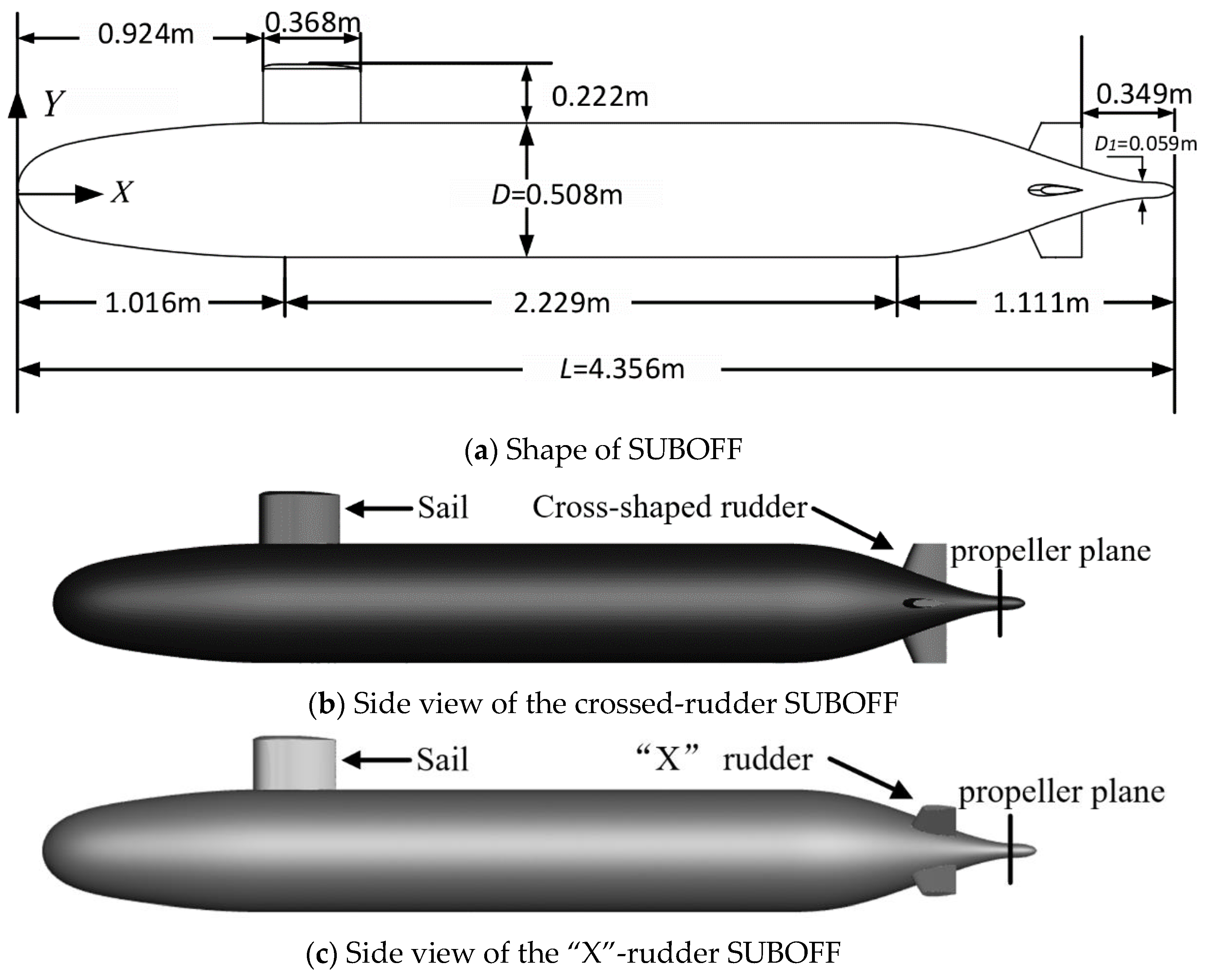
2.1. Submarine Model

The calculation model of this paper is based on the SUBOFF geometric model, published by the David Taylor Research Center in the U.S.A. [17]. The geometric dimensions under the Cartesian coordinate system are shown in Figure 2a. There are two primary components of the SUBOFF submarine: the main body and the attached body. As shown in

Table 1. Principal dimensions of SUBOFF.

Parameters	Value (m)
Total body length	4.356
Maximum body diameter	0.508
Forebody length	1.016
Parallel middle body length	2.229
Afterbody length	1.111
Total sail length	0.368
Total sail height	0.222
SUBOFF propeller plane diameter	0.059
Distance between the leading edge of the sail and the SUBOFF bow	0.924
Distance between the tail fin trailing edge and the SUBOFF stern	0.349

, the main body, i.e., the hull, as a rotating body, has a total length of L = 4.356 m, consisting of the forebody body, parallel middle body, and afterbody, with lengths of 1.016 m, 2.229 m, and 1.111 m, respectively, and the maximum body diameter of the hull is D = 0.508 m. The appendage contains the enclosing hull and the rudder (as shown in Figure 2b,c); the enclosing hull is a streamlined column with a height of 0.222 m and a length of 0.368 m, with the leading edge of a streamlined column. The enclosure is a streamlined column with a height of 0.222 m and a length of 0.368 m, and the leading edge is 0.924 m from the bow. The rudder consists of four rudder blades with NACA 0020 blades, and the trailing edge of the rudder blades is 0.349 m from the transom. There is a propeller plane at the transom of the submarine. The propeller plane is located at X/L = 0.978, and the diameter of the SUBOFF stern propeller plane is 0.059 m. The rudder types studied in this paper, as shown in Figure 2d,e, are crossed rudder and “X” rudder.

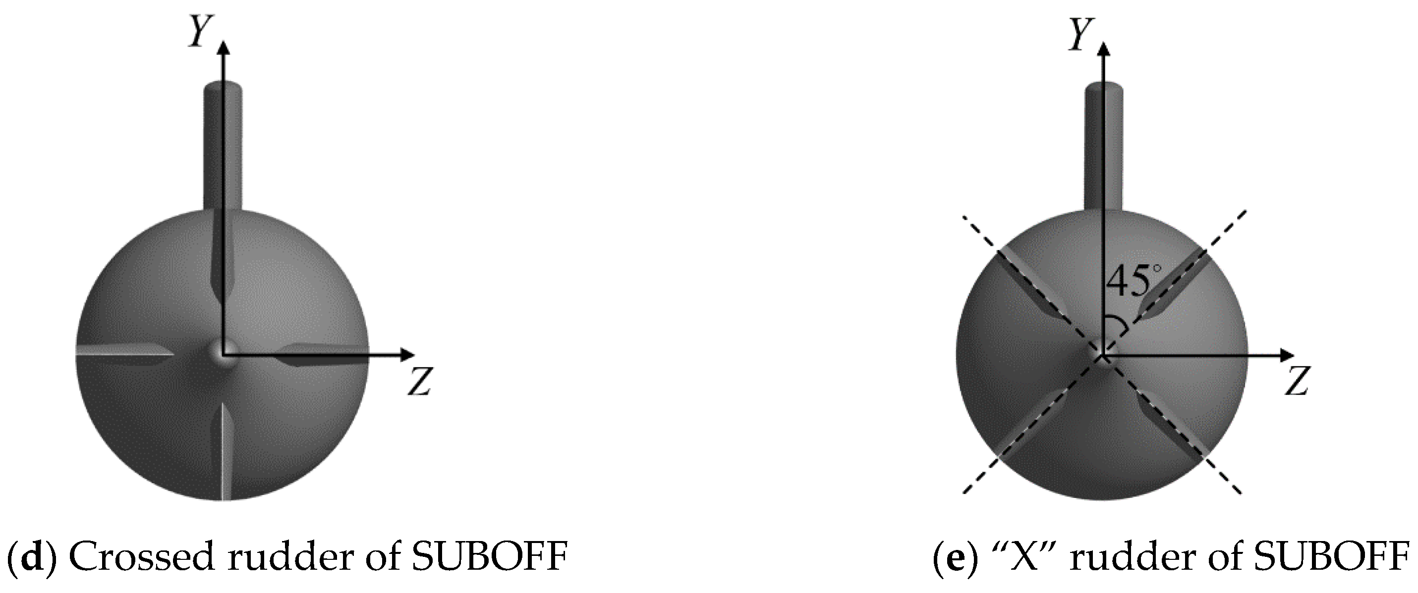
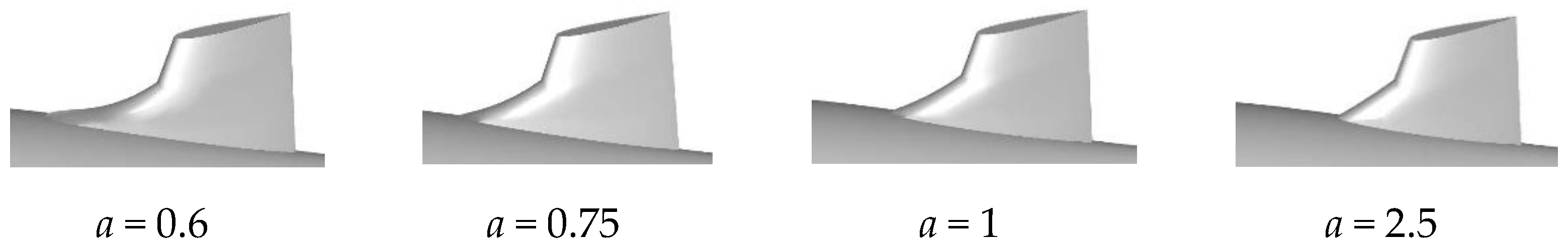
2.2. Design of the Stern Rudder with Fillets

As shown in Figure 3, the shortest length of the rudder blade profile is 0.152 m, and the angle between the leading-edge line and the x-axis is 65°. Now, take any point (x₀,y₀) of the leading-edge line of the rudder as the starting point for constructing the parabolic-type fillet.

The general form of a parabolic function is as follows:

$$y^2=-2ax$$

(1)

Equation (1) represents a parabola with an opening to the left, which is called the focal length of the parabola, whose value determines the size of the parabola’s opening. Since the rudder leading-edge line of the submarine has a certain angle of inclination, unlike the enclosure, which has an upright leading edge, it is necessary to rotate the parabola by a certain angle, according to the angle of inclination of the leading edge of the rudder, and translate it by a certain distance so that the vertex of the parabola is located at the position of (x₀,y₀). The formula for the rotation matrix in the Cartesian coordinate system is applied as follows:

$$M(\theta )=\left(\begin{array}{cc}\cos \theta & -\sin \theta \\ \sin \theta & \cos \theta \end{array}\right)$$

(2)

Type 2 for the rudder leading-edge tilt angle, in different submarine rudder fillet configurations, can be taken within the range of any angle, so the parabolic equation after rotating a certain angle is:

$${\left(x\sin \theta +y\cos \theta \right)}^2=-2a(x\cos \theta -y\sin \theta )$$

(3)

Now, by translating Equation (3), i.e., the vertex of the rotated parabola, to any point on the rudder leading-edge line, the final general form of the submarine rudder parabolic-type fillet can be obtained:

$${\left[(x-x_0)\sin \theta +(y-y_0)\cos \theta \right]}^2=-2a\left[(x-x_0)\cos \theta -(y-y_0)\sin \theta \right]$$

(4)

Equation (4), as a general form, can be used for any submarine attached to the leading edge of the submarine to construct a parabolic-type fillet.

It is known that the angle between the rudder leading-edge line and the x-axis in the SUBOFF submarine is 65°, so θ = 65°. Then, the midpoint of the rudder leading-edge line (3.831 m, 0.203 m) is taken as the starting point, and the parabolic corner filling of different sizes is constructed by taking four different focal lengths: 0.6, 0.75, 1, and 2.5. The specific corner-filling model is shown in Figure 4; L₁ to L₄ is the length of the forward extension of the corner filling, the dashed line indicates the original rudder blade configuration, and the modified shape is indicated by the solid line, in which the top shape of the modified corner filling remains the same as the top shape of the original blade configuration, i.e., the curvature of the solid and dashed lines of the top shape is the same. As the value increases, L₁ > L₂ > L₃ > L₄, i.e., the extension length decreases gradually, which is evident in the model diagram in Figure 5.

The SUBOFF model in this paper was built using the programming software MATLAB 2022b and the 3D modeling software SolidWorks 2022. Figure 5 explicitly illustrates the rudder fillet shapes for different values of a. It should be noted that the crossed rudders studied in this paper differ from “X”-shaped rudders only in the distribution of the rudder blades, while the shapes of the rudder blades are all as shown in Figure 5.

3. Numerical Methods

In this paper, the numerical simulation of a submarine with a speed of 7.161 m/s and a Reynolds number of 3.1 × 10⁷ is carried out using the fluid dynamics software ANSYS Fluent 2022 R1. The compressibility of the water is neglected in the calculation, and the thermal wake of the submarine is not involved, so it is not necessary to solve the equation for the conservation of energy, and the submarine wake flow field is described by solving the equation of continuity and the equation of momentum. In addition, the IDDES model is used as a turbulence modeling method to calculate the vorticity of the submarine’s transom flow field and the velocity distribution on the propeller plane. Fluent predicts the noise at the characteristic points using the FfowcsWilliams–Hawkings (FW-H) acoustic analysis module.

3.1. Fluid Motion Control Equations

Continuity equation [18]:

$$\nabla ·u=0$$

(5)

Momentum equation [18]:

$$\rho \left({\displaystyle \frac{\partial u}{\partial t}}+u·\nabla u\right)=-\nabla p+\mu {\nabla }^{2}u-\nabla ·{\tau }_{\mathrm{turb}}+f$$

(6)

$${\tau }_{\mathrm{turb}}=-\rho \overline{u_i^{\prime }{u}_j^{\prime }}$$

(7)

In Equation (6), $\rho$ denotes the fluid density and p represents pressure. µ denotes the dynamic viscosity of the fluid. τ_turb and f correspond to the Reynolds stress tensor and the volumetric force. The specific expression for τ_turb is given in Equation (7).

3.2. IDDES

The IDDES (Improved Delayed Detached Eddy Simulation) turbulence model is improved based on the original DES turbulence model. It mixes the RANS method and the LES method, which can better deal with the grid-induced separation problem, effectively analyze the small- and medium-scale turbulence structure in the separation region, and more accurately describe the reattachment location and morphological characteristics of the large-scale, time-averaged separating bubbles.

RANS is widely used in engineering, and its principle is to use the statistical theory of turbulence to time-average the unsteady N-S equations to solve the time-averaged quantities needed in engineering. The method decomposes the variables in the flow field into mean and pulsation values, and it solves the homogenized transport equations based on this decomposition. The momentum equation for its incompressible form is [19]:

$$\rho \left({\displaystyle \frac{\partial \overline{u_i}}{\partial t}}+\overline{u_j}{\displaystyle \frac{\partial \overline{u_i}}{\partial x_j}}\right)=-{\displaystyle \frac{\partial \overline{p}}{\partial x_i}}+\mu {\displaystyle \frac{{\partial }^2\overline{u_i}}{\partial x_j^2}}-{\displaystyle \frac{\partial }{\partial x_j}}\rho \overline{u_i^{\prime }{u}_j^{\prime }}+\rho f_i$$

(8)

In Equation (8), ${\displaystyle \frac{\partial \overline{u_i}}{\partial t}}$ is the time derivative term, which represents the rate of change in the mean velocity with time, reflecting the non-stationary nature of the flow; $\overline{u_j}{\displaystyle \frac{\partial \overline{u_i}}{\partial x_j}}$ is the convective term, which is the momentum transport due to fluid motion; ${\displaystyle \frac{\partial \overline{p}}{\partial x_i}}$ is the pressure gradient term, which represents the change in momentum driven by the pressure difference, which is the main driving force of the flow; $\mu {\displaystyle \frac{{\partial }^2\overline{u_i}}{\partial x_j^2}}$ is the viscous term, which is the diffusion of momentum due to the viscosity of the molecules; and $-{\displaystyle \frac{\partial }{\partial x_j}}\rho \overline{u_i^{\prime }{u}_j^{\prime }}$ is the Reynolds stress term, which represents the effect of turbulent pulsation on the mean momentum. The Reynolds stress is mainly dealt with by means of the eddy viscosity model, i.e., the turbulent viscosity is introduced, and the term is expressed in terms of the turbulent viscosity function. The relationship between the Reynolds stress and mean velocity gradient is established as [20]:

$$-\rho \overline{u_i^{\prime }{u}_j^{\prime }}={\mu }_t\left({\displaystyle \frac{\partial {\overline{u}}_i}{\partial x_j}}+{\displaystyle \frac{\partial u_j}{\partial x_i}}\right)-{\displaystyle \frac{2}{3}}\left(\rho k+{\mu }_t{\displaystyle \frac{\partial {\overline{u}}_i}{\partial x_i}}\right){\delta }_{ij}$$

(9)

$$k={\displaystyle \frac{\overline{u_i^{\prime }{u}_j^{\prime }}}{2}}$$

(10)

In Equations (9) and (10), u_t is the turbulent viscosity, k is the turbulent kinetic energy, and δ_ij is the sign of determination; δ_ij = 1 when i = j, and δ_ij = 0 when i ≠ j.

According to the number of turbulent viscosity ut solution equations, the eddy viscosity model can be categorized into a zero-equation model, a one-equation model, and a two-equation model. Currently, two-equation models are most widely used in engineering applications, mainly the standard k-ε model, the k-ω model, and the SST k-ω model.

In the k-ε model, the equations for the turbulent kinetic energy k and the turbulent dissipation rate ε are [21]:

$${\displaystyle \frac{\partial (\rho k)}{\partial t}}+{\displaystyle \frac{\partial (\rho k{u}_j)}{\partial x_j}}=P_k-\rho \epsilon +{\displaystyle \frac{\partial }{\partial x_j}}\left[\left(\mu +{\displaystyle \frac{{\mu }_t}{{\sigma }_k}}\right){\displaystyle \frac{\partial k}{\partial x_j}}\right]$$

(11)

$${\displaystyle \frac{\partial (\rho \epsilon )}{\partial t}}+{\displaystyle \frac{\partial (\rho \epsilon u_j)}{\partial x_j}}=C_{\epsilon 1}{\displaystyle \frac{\epsilon }{k}}{P}_k-C_{\epsilon 2}\rho {\displaystyle \frac{{\epsilon }^2}{k}}+{\displaystyle \frac{\partial }{\partial x_j}}\left[\left(\mu +{\displaystyle \frac{{\mu }_t}{{\sigma }_{ϵ}}}\right){\displaystyle \frac{\partial \epsilon }{\partial x_j}}\right]$$

(12)

where P_k in Equations (11) and (12) is the turbulent kinetic energy generation term.

In the k-ω two-equation model, the equations for turbulent kinetic energy k and the specific dissipation rate ω are [22]:

$${\displaystyle \frac{\partial (\rho k)}{\partial t}}+{\displaystyle \frac{\partial }{\partial x_j}}(\rho u_{j}k)={\displaystyle \frac{\partial }{\partial x_j}}\left[\left(\mu +{\displaystyle \frac{{\mu }_t}{{\sigma }_k}}\right){\displaystyle \frac{\partial k}{\partial x_j}}\right]+p_k-{\beta }^{\prime }\rho k\omega +p_{kb},$$

(13)

$${\displaystyle \frac{\partial (\rho \omega )}{\partial t}}+{\displaystyle \frac{\partial }{\partial x_j}}(\rho u_j\omega )={\displaystyle \frac{\partial }{\partial x_j}}\left[\left(\mu +{\displaystyle \frac{{\mu }_i}{{\sigma }_{\omega }}}\right){\displaystyle \frac{\partial \omega }{\partial x_j}}\right]+\alpha {\displaystyle \frac{\omega }{k}}{p}_k-\beta \rho {\omega }^2+p_{\omega b}$$

(14)

where p_kb and p_ωb in Equations (13) and (14) are turbulent kinetic energy buoyancy generation terms.

In submarine noise simulation, RANS (e.g., k-epsilon or k-omega) provides a steady-state flow field and low-frequency noise prediction with low computational cost, but k-epsilon is prone to underestimating the near-wall separation noise, and k-omega, which is better at curvilinear flow, is still not able to resolve high-frequency vortex sound. IDDES integrates the RANS and LES methods, dynamically adjusts the model to match the grid, maintains high efficiency in solving the boundary layer, and enhances the capability of capturing the broadband noise in the separation zone, which balances the accuracy and cost. Thus, it has become the preferred choice for the submarine’s complex acoustic scenarios. The following is a description of the transformation of DES into IDDES.

DES is a hybrid approach that combines the solution characteristics of RANS in the near-wall region and LES in the far field. The model switches between LES/RANS by modifying the scale of the dissipation term in the RANS equations.

The transport equation for the DES-modified turbulent viscosity $\tilde{\nu }$ is [23]:

$${\displaystyle \frac{\partial \tilde{\nu }}{\partial t}}+u·\nabla \tilde{\nu }=C_{b1}\tilde{S}\tilde{\nu }-C_{w1}{f}_w{\left({\displaystyle \frac{\tilde{\nu }}{L_{\mathrm{DES}}}}\right)}^2+{\displaystyle \frac{1}{\sigma }}\left[\nabla ·((\nu +\tilde{\nu })\nabla \tilde{\nu })+C_{b2}{(\nabla \tilde{\nu })}^2\right]$$

(15)

where $\tilde{S}$ is the corrected vortex, which is given by:

$$\tilde{S}=\sqrt{2{\mathsf{\Omega }}_{ij}{\mathsf{\Omega }}_{ij}}+{\displaystyle \frac{\tilde{\nu }}{{\kappa }^2{d}^2}}{f}_{v2}$$

(16)

where ${\mathsf{\Omega }}_{ij}$ is the rotation tensor.

The length scale for the DES turbulence model is defined as follows [24]:

$$L_{DES}=\min \{d,L_{LES}\}$$

(17)

The LES length size expression is [24]:

$$L_{LES}=C_{DES}\Delta$$

(18)

where the expression for $\Delta$ is:

$$\Delta =\max \{\Delta x,\Delta y,\Delta z\}$$

(19)

In Equation (17), d is the shortest distance from the wall. In Equation (18), $\Delta$ it is the maximum value of the local mesh size in all three directions. C_DES is a model constant. C_DES = 0.65. In Equation (17), it can be seen that the conversion from RANS to LES depends entirely on the mesh scale size. In some cases, it can lead to the early conversion of RANS to LES and the model stress dissipation phenomenon, which leads to GID (grid-induced separation). Scientists have tried to solve this problem by proposing DDES (Delayed Detached Eddy Simulation). The DDES length size expression is [24]:

$$L_{\mathrm{DDES}}=d-f_{\mathrm{d}}\max \left(0,d-\psi C_{DES}\Delta \right)$$

(20)

where f_d in Equation (20) is the delayed transition function that prevents the LES from being solved within the boundary layer, thus solving the GID problem. While DDES still cannot solve the problem of log-layer mismatch inside the boundary layer, the IDEES method has been further developed. The IDDES length size expression is [24]:

$$L_{\mathrm{IDDES}}=f_{\mathrm{d}}\left(1+f_{\mathrm{e}}\right)d+\left(1-{\tilde{f}}_{\mathrm{d}}\right)\psi C_{\mathrm{DES}}{\Delta }_1$$

(21)

In Equation (21),

$${\Delta }_1=\min \left(\max \left(0.15d,0.15\Delta ,{\Delta }_{\min }\right),\Delta \right)$$

(22)

$${\tilde{f}}_{\mathrm{d}}=\max \left(\left(1-f_{dt}\right),f_B\right)$$

(23)

$$f_{dt}=1-\tanh \left[{\left(C_{dt}{r}_{dt}\right)}^3\right]$$

(24)

$$r_{dt}={\displaystyle \frac{\upsilon }{k^2{d}^2·\max \left\{{\left[{\displaystyle \sum _{i,j}{\left(\partial u_i/\partial x_j\right)}^2}\right]}^{1/2},{10}^{-10}\right\}}}$$

(25)

where the subscripts d and e are the symbols associated with the delay function and the rise function, respectively. In Equations (21)–(25), ${\mathsf{\Delta }}_{\mathrm{m}\mathrm{i}\mathrm{n}}$ is the minimum distance from the center of the grid to adjacent grids, ψ is the low Reynolds number correction function, υ is the kinematic viscosity coefficient, $\partial u_i/\partial x_j$ is the velocity gradient, C is the mixing function, C_dt is the model constant, and f_e is the transformation function.

IDDES effectively solves the problems of model stress dissipation and log-layer mismatch arising from DES methods when dealing with large separation flows, thus improving the numerical solution accuracy of large separation flows at high Reynolds numbers.

3.3. The FW-H Equation

In terms of the governing equations, FW-H equations are an exact reorganization of the continuity and momentum equations in fluid dynamics. The acoustic modular equations used in ANSYS Fluent are generalized FW-H equations, which are specifically expressed as [25]:

$$\begin{array}{c}{\displaystyle \frac{1}{e_0^2}}{\displaystyle \frac{{\partial }^2{p}^{\prime }}{\partial t^2}}-{\nabla }^2{p}^{\prime }={\displaystyle \frac{{\partial }^2}{\partial x_i\partial x_j}}\left[T_{ij}H(f)\right]-{\displaystyle \frac{\partial }{\partial x_i}}\left\{\left[P_{ij}{n}_j+\rho u_i\left(u_n-v_n\right)\right]\delta (f)\right\}\\ +{\displaystyle \frac{\partial }{\partial t}}\left\{\left[{\rho }_0{v}_n+\rho \left(u_n-v_n\right)\right]\delta (f)\right\}\end{array}$$

(26)

In Equation (26), e₀ is the far-field sound velocity; p′ is the sound pressure; δ(f) and H(f) are the Dirac delta function and Heaviside function, respectively; f is the wall function; $\rho$ is the density; ${\rho }_0$ is the far-field density; T_ij is the Lighthill stress tensor; P_ij is the compressive stress tensor; and n is the direction normal to the outside of the wall that points inside the fluid and contains the component n_j. u_i is the component of the fluid velocity in the x_i direction; u_n is the component of the fluid velocity in the direction normal to the wall; v_i is the component of the surface velocity in the x_i direction; and v_n is the component of the surface velocity along its normal direction.

The numerical calculation of submarine flow noise is a moving solid boundary problem, which requires the use of the FW-H equation to calculate the far-field noise. Wang’s work [8] shows that for the numerical calculation, submarine flow noise can be accurately simulated by using the FW-H equation. Therefore, in this paper, the FW-H equations are used to calculate the sound source parameters calculated from the flow field transients of the IDDES method in order to accurately simulate the submarine far-field noise numerically.

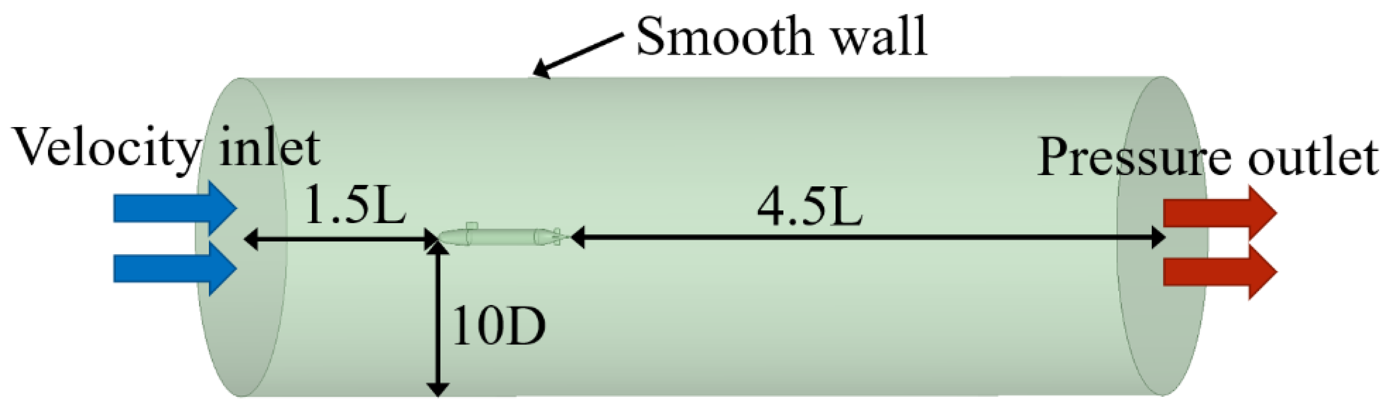
3.4. Computational Domain and Boundary Conditions

As the submarine approaches the outlet, the fluid in the wake (near the outlet end) accelerates out of the submarine, resulting in a lower pressure in the wake. The lower pressure reduces the pressure difference between the front and rear of the submarine (the main source of differential pressure drag), thus reducing the total force. The fluid domain is too large to waste computational resources. Therefore, choosing an appropriate fluid domain can better simulate the submarine wake flow situation. In this paper, a sensitivity analysis of submarine drag is performed on three key parameters, which are the distance between the submarine’s bow and the inlet of the fluid domain (L_i), the distance between the submarine’s stern and the outlet of the fluid domain (L_o), and the radius of the cylindrical fluid domain (D_w). The results of the sensitivity analysis in Figure 6 show that a change in the size of the fluid domain affects the submarine drag and, thus, the wake development. Finally, in this paper, the fluid domains of L_i = 1.5L, L_o = 4.5L, and D_w = 10D are selected for numerical calculations, which can avoid the secondary perturbation to the submarine caused by too-small fluid domains.

The cylindrical domain is taken as the numerical computational domain of the submarine, and the specific parameters are shown in Figure 7. L denotes the overall length of the submarine and D denotes the maximum diameter of the submarine (L = 4.356 m, D = 0.508 m). The total length of the computational domain is 7L, the inlet is 1.5L from the bow, and the outlet is 4.5L from the transom. The radius of the cylindrical domain is 10D. The boundary conditions are defined as the velocity inlet boundary condition and the pressure outlet boundary condition, the submarine surface is defined as a no-slip boundary condition, and the wall surface is defined as a zero-shear–slip wall surface.

Table 2. Working condition parameters.

Parameter	Setting Situation
Computational domain material	Liquid water
Inlet	Velocity inlet (7.161 m/s)
Outlet	Pressure outlet
Computational domain wall	Smooth wall
SUBOFF wall	No-slip wall

lists, in detail, the boundary conditions for the computational cases. It is worth noting that this paper studies the submarine while sailing in seawater inside the bypass flow, so it does not consider the effect of the free liquid surface, unlike Park et al. [26], on the inlet. The velocity inlet uses the top, bottom, and side boundaries. This paper considers the side boundaries in using a smooth wall, which removes the need to consider the roughness caused by an additional turbulence effect, thus improving the efficiency of the calculation.

Table 3. Solver settings.

Parameters	Setting Situation
Turbulence model (transient calculation)	IDDES
Acoustical model	FW-H
y+	0.9 < y+ < 1
Pressure–velocity coupling scheme	SIMPLE
Momentum	Second-order upwind
Turbulent kinetic energy	Second-order upwind
Turbulent dissipation rate	Second-order upwind
Transient formulation	Second-order implicit
Reference sound pressure	1 × 10−6 Pa
Sound source	SUBOFF model surface
Type of sound source	Wall
Convergence criteria (drag detection)	Drag change < 0.1% over 100 consecutive iterations
Maximum number of iterations/time step	20
Maximum analysis frequency	1000 Hz
Transient calculation time step	5 × 10−4 s
Under relaxation factor	Pressure: 0.3 Momentum: 0.7 Turbulent kinetic energy: 0.8 Turbulent dissipation rate: 0.8

provides detailed information about the solver settings. It is worth noting that this paper uses the FW-H acoustic model with the SUBOFF surface as the wall-type sound source. The reference sound pressure in water is 1 × 10⁻⁶ Pa. In this paper, submarine drag is used as the monitoring physical quantity, and convergence is determined when the rate of change in the resistance is less than 0.1% for 100 consecutive steps.

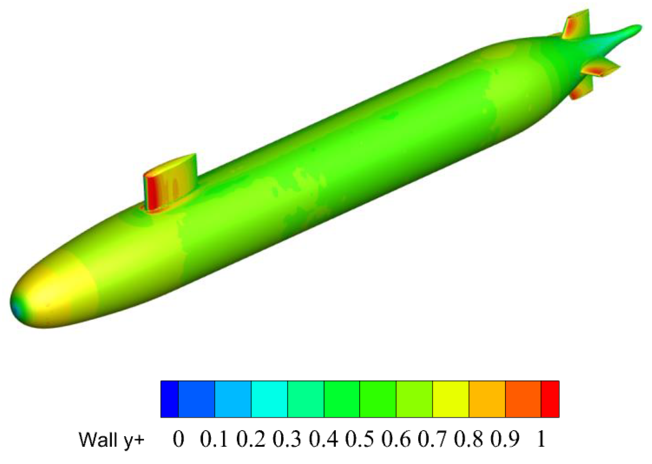
3.5. Grid Independence Verification

ANSYS Fluent Meshing is utilized for the mesh. The whole set of submarine mesh is a hybrid mesh with mesh encryption for the submarine’s near-flow and wake-flow fields, as shown in Figure 8a. Figure 8b,c show the details of the envelope and rudder blade meshes of the SUBOFF submarine, respectively. This paper also implements a mesh expansion layer over the entire surface of the SUBOFF submarine, and Figure 8d,e show the mesh expansion around the sail and rudder.

In fluid dynamics and computational fluid dynamics, y⁺ is a dimensionless parameter that describes the resolution of the mesh near the wall and its relationship with the turbulent boundary layer. The expression is as follows [27]:

$$y^{+}={\displaystyle \frac{{\rho }_{w}y{u}_{\tau }}{{\mu }_w}}$$

(27)

$$u_{\tau }=\sqrt{{\displaystyle \frac{{\tau }_w}{\rho }}}$$

(28)

In Equation (27), y denotes the actual distance from a point of the fluid to the wall, ${\rho }_w$ and µ_w denote the density and dynamic viscosity of seawater near the surface of the SUBOFF submarine, and u_τ denotes the wall friction velocity, the expression of which is shown in Equation (28). τ_w in Equation (28) is the wall shear stress.

Figure 9 exhibits the y⁺ values for the SUBOFF submarine, where y⁺_max = 0.97. y⁺ is the dimensionless wall distance, which is crucial in turbulence simulation, and its value reflects the fineness of the near-wall mesh, which directly affects the resolution accuracy of the flow features within the boundary layer. In IDDES (Improved Delayed Separation Eddy Simulation), a reasonable setting of y⁺ (y⁺ ≤ 1 in the near-wall region) ensures the accuracy of the RANS (Reynolds Averaged Navier–Stokes) model near the wall, which can effectively simulate the flow in the viscous sublayer and logarithmic law region. Away from the wall, IDDES dynamically switches to the LES (Large Eddy Simulation) mode through the delay function to resolve the large-scale eddy structure. y⁺ (dimensionless wall distance) is the most important factor in the turbulence simulation. The optimization of y⁺ not only ensures the smoothness of the RANS-LES transition, but it also balances the computational cost and accuracy.

This paper uses six sets of grid quantities of different sizes for grid independence validation, with the amounts increasing from millions to tens of millions. The submarine resistance is calculated for different grid quantity sizes at an incoming flow velocity of 3.05 m/s. The detailed results are shown in

Table 4. Submarine resistance values for a different number of grids.

Grid	Number of Grids (×104)	Force (N)	Nodes (×104)	GCI (%)	Skewness
Grid A	242.5	105.4	464.0	11.32	0.66
Grid B	545.2	104.3	739.9	7.61	0.61
Grid C	850.0	103.0	1305.8	4.84	0.55
Grid D	1192.1	102.5	2072.6	1.22	0.62
Grid E	1406.9	102.4	2879.2	1.15	0.56
Grid F	1721.5	102.4	3564.5	1.14	0.57

.

As shown in Table 4, the submarine resistance change trend gradually slows with an increase in the number of grids. It is almost unchanged at the end, indicating that further growth in the number of grids no longer significantly affects the numerical calculation results. The GCI from grid D to grid F is less than 3%. To consider computational accuracy and grid computing resources, grid E, i.e., with a total number of 14,069,000 grids, is selected for the numerical simulation calculation. It is with this number of grids (grid E) that Figure 8 is realized.

3.6. Numerical Validation

The experimental data on the two physical quantities of the pressure coefficient and force are compared with the numerical calculation data to verify the reliability of the numerical calculation method used in this paper. The following formula is used to calculate the pressure coefficient:

$$C_P={\displaystyle \frac{P-P_{ref}}{0.5{\rho }_{ref}{v}_{ref}^2}}$$

(29)

where C_p is the pressure coefficient; P is the static pressure; P_ref is the reference pressure; ρ_ref is the reference density; and v_ref is the reference incoming velocity.

As shown in Figure 10, the numerical simulation values of the pressure coefficient are in good agreement with the experimental values at the forebody and parallel midbody sections. However, near the sail leading edge and the rudder leading edge, there are slight discrepancies between the peak and trough values obtained from the numerical simulations and experiments. The reason for these discrepancies is that the flow is impeded at these locations, causing a sudden decrease in the incoming flow velocity and a sharp increase in pressure.

The submarine’s resistance to navigation for six groups of different speeds is calculated using grid E and compared with the experimental values to obtain the relative errors. As can be seen in

Table 5. Calculated and experimental values of force at different speeds.

Speed (m/s)	Experimental Value (N)	Calculated Value (N)	Relative Error (%)
3.051	102.3	102.6	0.3
5.144	283.8	289.1	1.8
6.096	389.2	396.8	1.9
7.161	526.6	529.0	0.4
8.231	675.6	693.8	2.7
9.152	821.1	840.9	2.4

, the maximum relative error is only 2.7%.

In terms of noise research, this paper numerically calculates the SUBOFF model for the incoming flow velocity working condition of 3.05 m/s and analyzes it compared with the experimental results. The calculation results show that the total sound pressure level at the characteristic point (2.178, −2, 0) is 100.9 dB, closer to the experimental value of 101.3 dB.

Overall, the IDDES turbulence model is used to calculate the submarine winding flow field and the numerical calculation results are compared with the experimental results. The agreement is high, and the error is small, which reflects the feasibility and accuracy of the calculation method used in this paper.

4. Results and Discussion

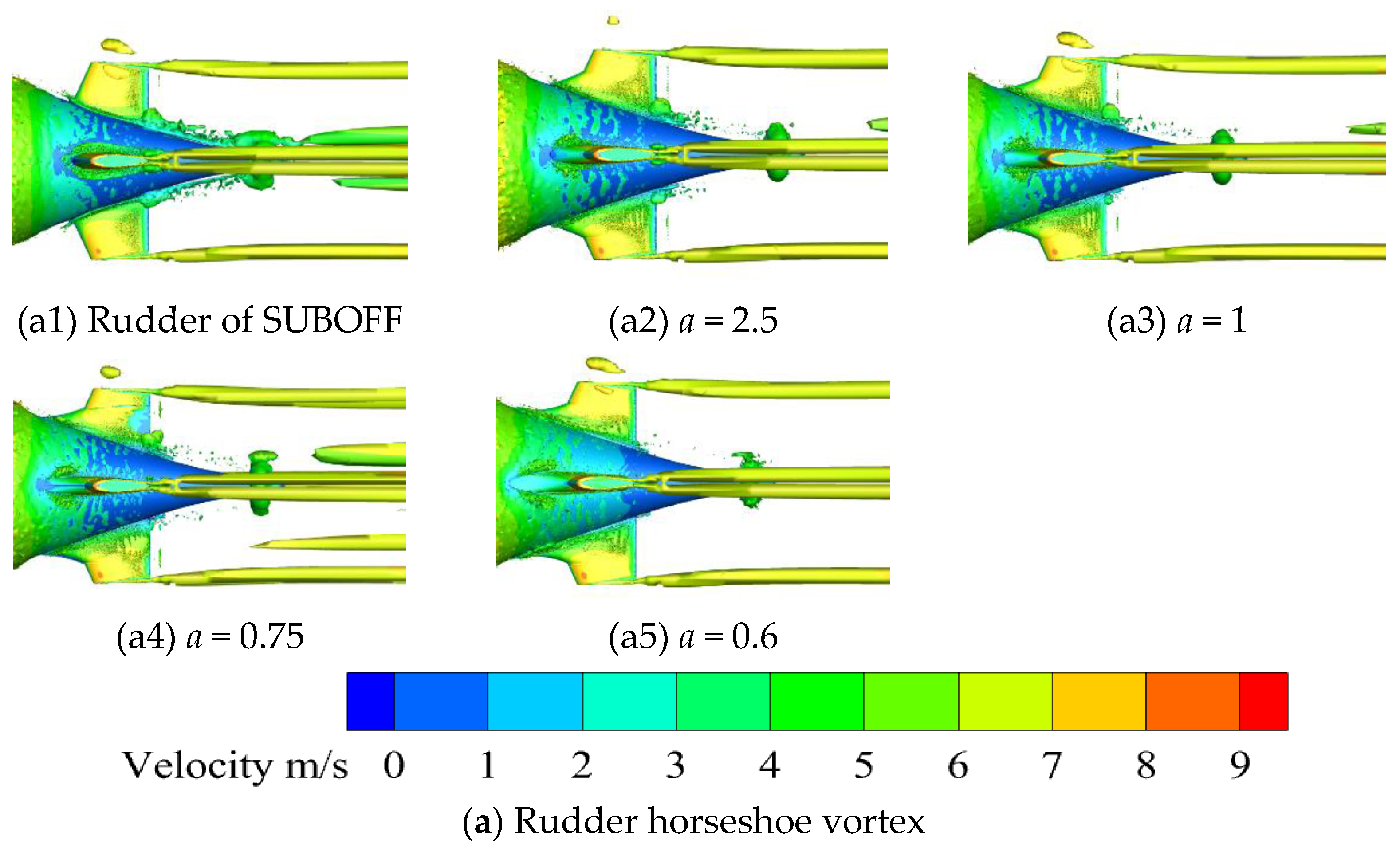
4.1. Effect of Rudders on Submarine Stern Vortices

In the process of submarine navigation, the existence of the attached body will inevitably lead to the generation of various vortices, such as the horseshoe vortex, the tip vortex, the tail vortex, and so on. Among them, the horseshoe vortex and the wake vortex at a submarine’s transom are the most obvious, which have a significant effect on the hydrodynamic characteristics of the submarine.

Figure 11 shows the distribution of vortices around the rudders of five crossed rudders with different fillets. The computational conditions of the five models are the same, and the speed is 7.161 m/s. The Q-criterion (Q = 1.5 s⁻²) is utilized to represent the vortex structure on the isoparametric surface rendered by the flow velocity.

From the distribution of horseshoe vortices in the rudder, as shown in Figure 11(a1), it can be seen that the leading edge of the prototype rudder, due to the tilted upright-type structure, clearly produces a horseshoe vortex with a U-shape structure at the root of the leading edge when it encounters a fluid impact. When the fluid flows through the rudder, a great counterpressure gradient is formed at the leading edge; the flow field undergoes obvious flow separation and produces a strong vortex flow, while the vortex drives the surrounding flow field to form a vortex tube extending to the transom. The transom of the submarine, due to its streamlined structure, causes the vortex tube to propagate further downstream. The horseshoe vortices of the four rudder blades eventually converge near the propeller plane to form a large vortex cluster, as shown in Figure 11(b1), which has a clear and obvious structure consisting of four small vortex clusters. Each of these small vortex clusters is formed by the convergence of two single vortex tubes from the two neighboring rudder blades. As the fluid flows through the submarine, the large vortex cluster at the propeller plane continues to extend backward.

The parabolic fillets, because of their unique linear structure, act as good deflectors and buffers when the fluid hits the leading edge of the rudder. In Figure 11(a2–a5), it can be seen that as the a-value decreases, i.e., the fillet structure increases, the degree of damage to the rudder’s horseshoe vortex structure grows, which means that the flow separation at the leading edge of the rudder is weakened, and the strength of the horseshoe vortex gradually decreases. As shown in Figure 11(b2–b5), the vortex tube extending from the horseshoe vortex becomes thinner due to the weakening of its strength. At the same time, this results in the large vortex cluster gathered at the stern propeller plane changing from a four-small-vortex-cluster structure at the beginning to a dissipated and destroyed irregular structure with a gradually decreasing volume. The strength of the wake vortex extending from the large vortex at the propeller plane is subsequently gradually weakened.

It is concluded that the addition of the corner-filling structure in the rudder of the submarine has a good effect on the suppression of the horseshoe vortex and the wake vortex structure in the rudder.

In Figure 12, it can be seen that increasing the fillets of appropriate size reduces the submarine force. This is because the vortex scale at the rudder–body junction decreases after increasing the fillet, the differential pressure force decreases, and the horseshoe vortex is suppressed, as can be seen in Figure 11. However, as the fillet increases, the force reduction rate gradually slows down, and even the force tends to increase, which indicates that too large a fillet will increase the force of the submarine. When comparing the crossed-rudder SUBOFF and the “X”-rudder SUBOFF, it is found that the force of the “X”-type is smaller than that of the cross-type under the same rudder. This indicates that the force performance of the “X”-rudder SUBOFF is better than that of the crossed-rudder SUBOFF under direct flight.

4.2. Effect of Rudder Distribution and Structure on Submarine Velocity Field

As the part of the submarine where the propeller is installed, the flow around the propeller plane greatly influences the propeller noise level. The higher the uniformity of the velocity distribution at the propeller plane, the more stable the flow situation around the propeller is, and the propeller noise is reduced. Therefore, for the velocity distribution at the submarine’s propeller plane, this paper investigates a submarine with different rudder distributions and fillets.

Figure 13 shows that all the velocity distributions at the submarine propeller plane surface are consistent with the rudder layout type. The velocity distribution contours of the crossed rudders in Figure 13(a1–a5) continue to extend in four directions, i.e., up, down, left, and right, while spreading outward from the center, presenting a cross shape. The velocity distribution contours of the “X”-shaped rudders in Figure 13(b1–b5) eventually extend in four directions as well, presenting an “X” shape.

In the region of higher speed (r/R > 0.5), the sparsity of the same rudder layout is almost the same, and the main difference lies in the low-speed region around the center of the propeller plane (0 < r/R < 0.5), which appears to have different shapes and different sparsity. Regardless of the rudder layout of the submarine, under the condition of no fillet, as shown in Figure 13(a1,b1), the contour distribution of the low-speed region is highly uneven, and there is an inward concavity, similar to the shape of a “four-leaf clover”. It can be seen that the fluid flow near the propeller plane surface is unstable at this time.

By increasing the fillet, it can be found that the velocity field at the propeller plane is dramatically improved. As shown in Figure 13(a2,b2), the fillet makes the contour lines in the low-speed region more sparse and uniform, and the concavity is slowed down so that it is no longer in the shape of a “four-leaf clover”. This is because the rudder fillet destroys the horseshoe vortex structure and, simultaneously, makes the two longitudinal vortices of the horseshoe vortex that originally developed backward weaken and enhance the flow stability of the transom fluid. The improvement becomes more and more evident as the value of a decreases, i.e., the fillet increases (e.g., Figure 13(a2–a5) vs. Figure 13(b2–b5)). Ultimately, the velocity distribution contour plots of the entire propeller plane show perfect symmetry and uniformity, and the contour distributions of the small velocity field tend to be internally uniform in the shape of concentric circles.

Through the above analysis, it can be seen that with the increase in the filling volume, the velocity contour uniformity at the propeller plane gradually grows, and the distribution of the flow field becomes more and more stable, especially for the lower-velocity region, which is the most apparent feature. Therefore, the fillet has a specific improvement effect on the flow field at the propeller plane of the submarine.

Figure 14 reveals a significant abrupt change in the axial velocity at the upper vertical rudder position of the crossed rudder. This may be due to the slow dissipation of the vortex generated by the enclosure extending to this rudder blade, which is equivalent to the dual action of the enclosure and the upper vertical rudder blade interfering with the velocity field at the propeller plane. On the other hand, the velocity fluctuation of the “X” rudder is relatively small due to its misalignment with the enclosure in the circumferential layout. Figure 14 shows the axial dimensionless velocity distributions of the submarine with two rudder layouts at r = 0.2R on the propeller plane. In this figure, it can be seen that there is a high-velocity region behind the rudder wing of both tail maneuvering surfaces, which is formed due to the horseshoe vortex that brings the higher velocity fluid from the outer radius region to the inner radius region.

Combined with Figure 14a,b, the peak values of axial companion velocities are decreased after adding the rudder fillet. The fillet at the root of the rudder breaks the horseshoe vortex structure, weakening its influence on the transom companion flow field.

Table 6. Comparison of ΔU_x between cross-shaped and “X”-shaped submarines at the r/R = 0.3 propeller plane.

	ΔUx		Reduced Magnitude (%)
	Cross-Shaped	“X”-Shaped
SUBOFF	0.18234	0.10993	39.71
a = 2.5	0.10789	0.05466	49.34
a = 1	0.07688	0.05078	33.95
a = 0.75	0.07049	0.04891	30.61
a = 0.6	0.05175	0.03871	25.20

shows that in the r = 0.3R propeller plane circumferential low-speed region, the difference between the peak and valley values of the propeller plane circumferential velocity of the “X” rudder is reduced by 39.71% compared with that of the cruciform rudder propeller plane. For the same rudder fillet of the same layout, the difference between the peak and valley values of the velocity of the “X” submarine is smaller than that of the cruciform submarine. For the same rudder fillets and different layouts, the difference between the peak and valley values of the “X” submarine is smaller than that of the crossed submarine, which indicates that the wake quality of the “X” submarine is significantly improved compared with that of the crossed submarine.

Secondly, after adding the rudder fillet, the wake quality is still improved, and the maximum reduction reaches 49.34%. With the decrease in the a value, i.e., the increase in the filler angle volume, the difference between the peak and valley values of the circumferential velocity on the propeller surface decreases. Still, the reduction gradually decreases from 49.34% to 25.20%. This indicates that although the fillet can improve the wake quality, the reduction will no longer be noticeable when the fillet reaches a specific size.

Overall, the flow quality of the “X”-rudder submarine is better than that of the crossed-rudder submarine at the propeller plane, especially in the low-speed region around the propeller plane. The optimization of the wake flow helps to reduce the excitation vortex of the propeller, which, in turn, reduces the vibration and noise of the propeller.

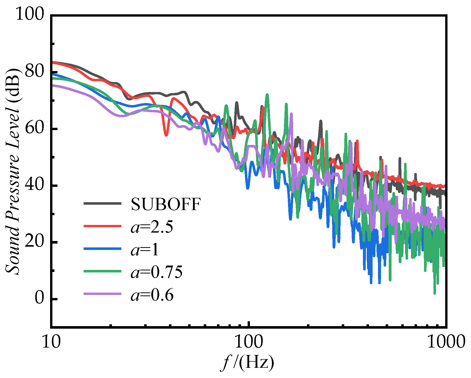
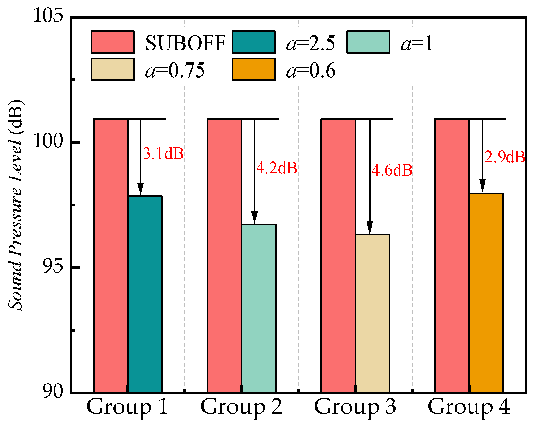
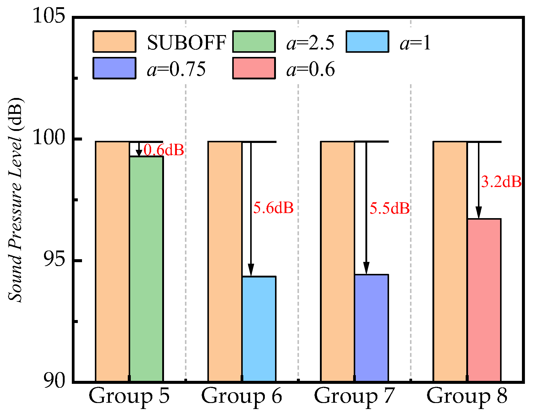
4.3. Effect of Rudder Fillets on Submarine Hydrodynamic Noise

Figure 15 and Figure 16 present a comparison of the spectral curves of sound pressure levels at the characteristic point (2.178, −2, 0) for a crossed-rudder submarine and an “X”-rudder submarine, respectively. The hydrodynamic noise generated by the submarine covers a wide frequency range and is a typical broadband noise. The radiated energy of this noise is mainly concentrated in the low-frequency band, where the low-frequency noise dominates, while the high-frequency noise is relatively less.

In Figure 15, it can be seen that compared with the prototype rudder, the noise level in the low-frequency band (especially below 100 Hz) of the cruciform rudder containing the fillet design is significantly reduced. This indicates that the corner-filling design is effective in suppressing the generation of low-frequency noise. However, in the high-frequency region, there is a slight increase in the noise level. This increase in high-frequency noise may be due to the complexity of the propagation and distribution of high-frequency noise in the flow field, which mainly originates from the fine eddy structures in the turbulent flow and the high-frequency pulsations of the fluid. These high-frequency noise sources are more dispersed and are difficult to be eliminated completely by the simple design of fillets. In Figure 14, except for the rudder fillets with a = 2.5, the rest of the fillets show good noise reduction characteristics in both the low- and high-frequency bands. The a = 2.5 rudder fillets are smaller in size, and their suppression effect on horseshoe vortices is relatively weak; however, they still have some noise reduction effect, but not as obvious as the other fillets. In contrast, the other three rudder fillets not only can effectively suppress the horseshoe vortex, but also, according to the analysis in Section 4.2, the “X”-rudder submarine can more effectively improve the uniformity of the wake flow field, so the “X”-rudder fillet has a more significant noise reduction effect.

In addition, it can be seen in Figure 16 that the fillets with a = 0.75 and a = 1 are significantly better than those with a = 2.5 in terms of noise reduction performance. This is due to the fact that a fillet with too large a volume may disrupt the flow structure and trigger additional flow separation or vortex shedding, which, in turn, weakens the noise reduction effect. This phenomenon suggests that the noise reduction effect of the fill angle is not monotonically enhanced with the increase in volume.

Figure 17 and Figure 18 clearly show a comparison of the total sound pressure level of a submarine with and without rudder fillets. Groups 1 through 4 in Figure 17 are crossed rudders, and Groups 5 through 8 in Figure 18 are “X” rudders. It can be seen that the hydrodynamic noise of the submarine is generally reduced with the addition of fillets at the leading edge of the rudder. Specifically, the crossed-rudder fillets can reduce the hydrodynamic noise of the submarine by up to 4.6 decibels (dB), while the “X”-rudder fillets can reduce the noise by up to 5.6 dB. This is mainly due to the fact that the fillets can effectively inhibit the formation of a horseshoe vortex, thus reducing the noise. However, as the value of the fillet parameter decreases, i.e., the value of the tail chord length L increases, the noise reduction effect gradually decreases. This is because a larger tail chord length leads to an increase in the noise of the rudder blade airfoil shape, which partially offsets the noise reduction effect brought by the fillet. In addition, the volume and shape of the fillets also have a significant effect on the noise reduction effect. For example, fillets of a = 1 and a = 0.7 are significantly better than a fillet of a = 2.5 in terms of noise reduction. This indicates that the design of the fillet needs to consider its volume and shape comprehensively to achieve the best noise reduction effect. Therefore, when designing fillets, not only the suppression of the horseshoe vortex, but also its effect on the uniformity of the wake field, should be considered to realize the best hydrodynamic performance and noise control.

5. Conclusions

(1)

In this paper, a general line equation for corner filling is derived based on the parabolic equation, which constructs corner-filling-type lines that can be used for most submarine attachments.

(2)

Using the IDDES model and comparing the simulation and test results, the drag force’s relative error is only 2.7%, at maximum, at different speeds. The distribution of the pressure coefficient along the upper surface of the SUBOFF submarine is highly consistent with the test results, indicating that the results computed by the IDDES model have high realism and reliability.

(3)

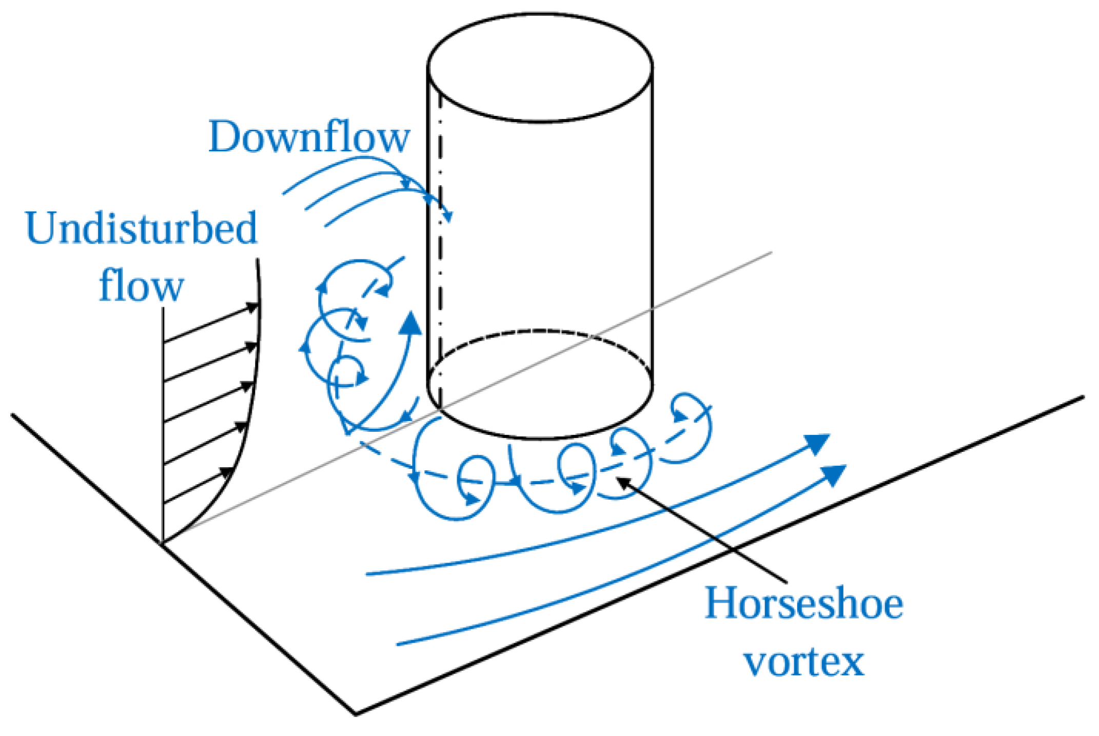
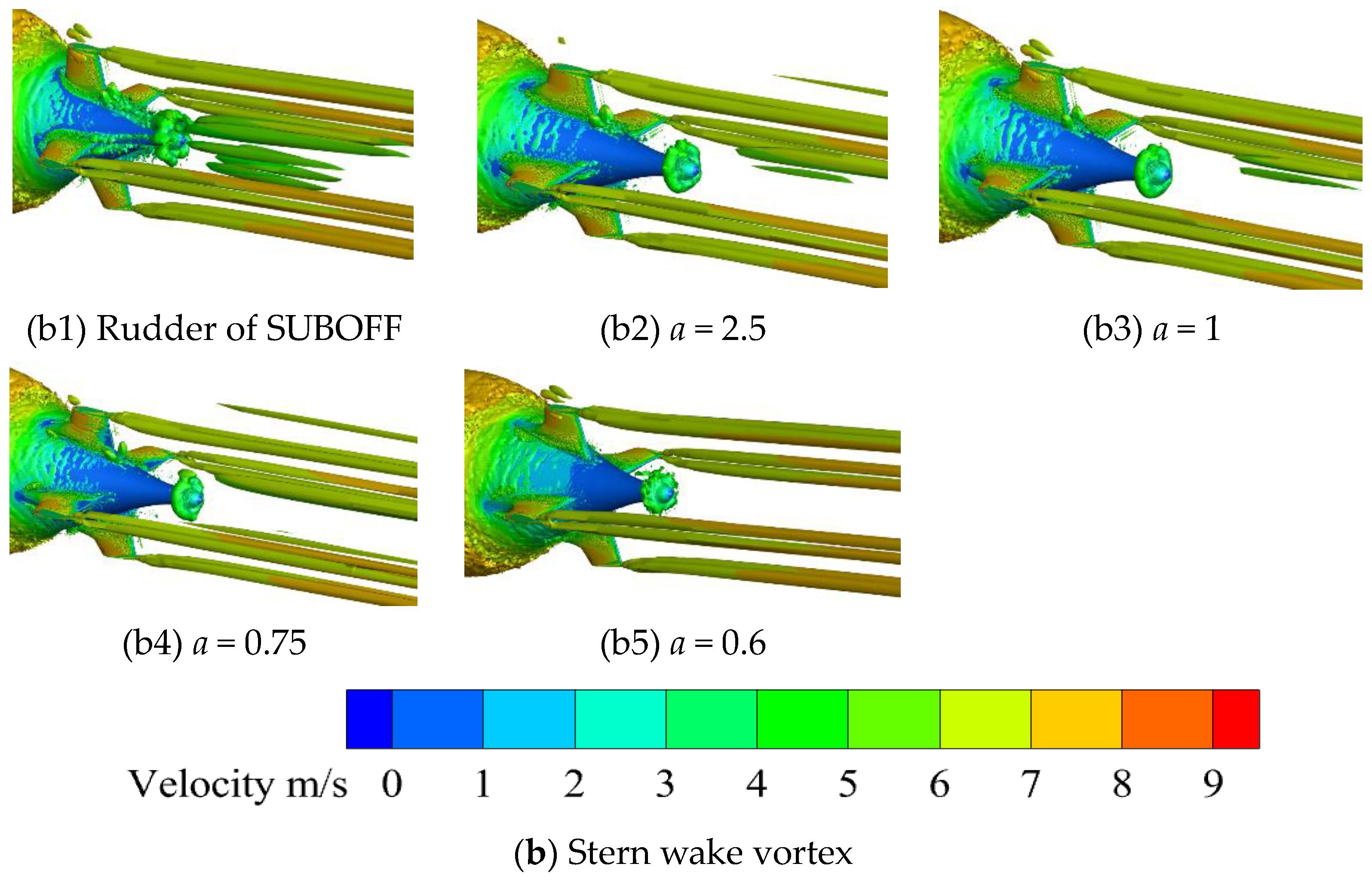
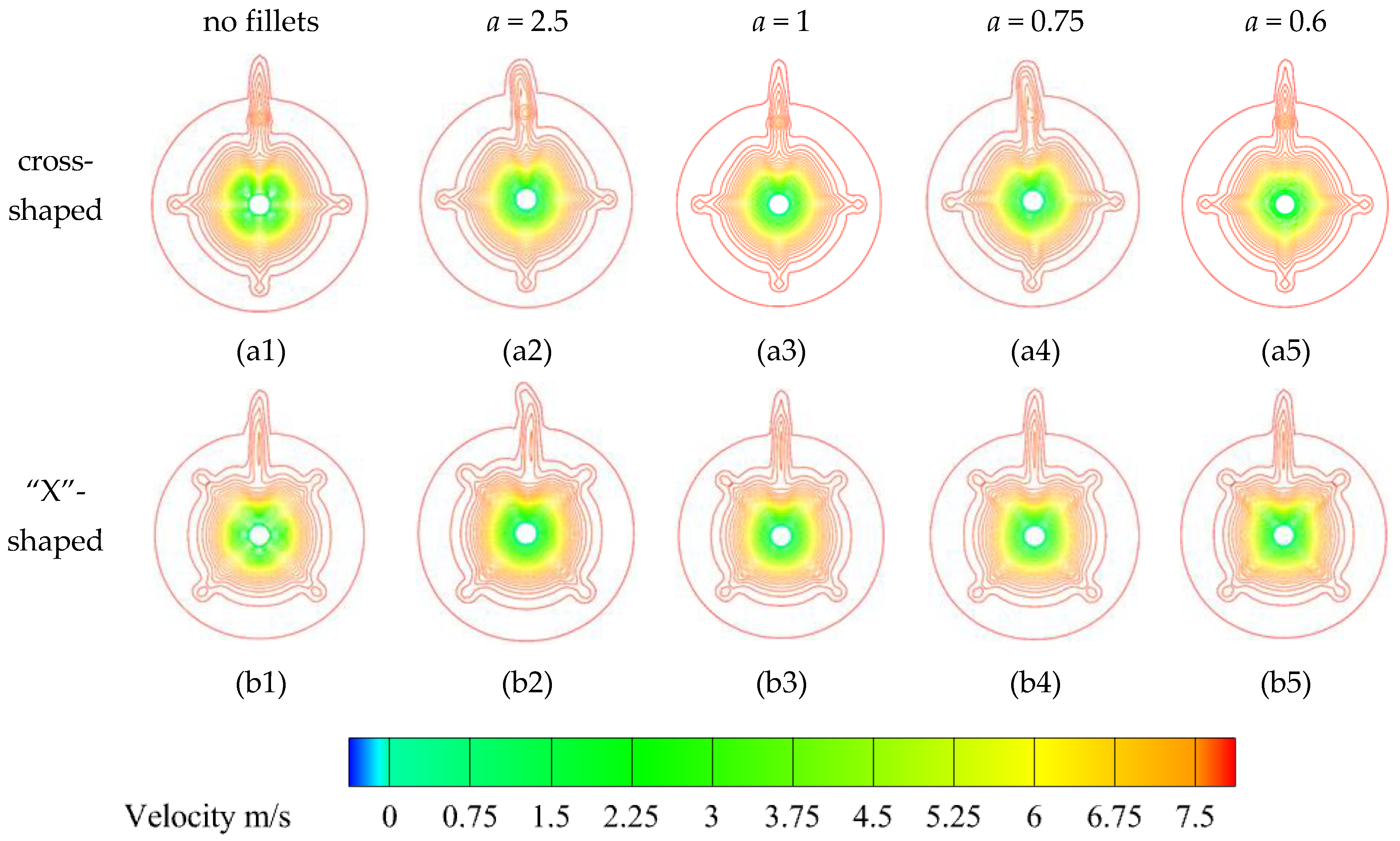
For both crossed-rudder and “X”-rudder submarines, increasing the fillet disrupts the horseshoe vortex structure, effectively suppressing its adverse effects (e.g., flow separation and turbulence generation) and improving the wake flow field. Notably, the “X” rudder demonstrates superior performance over the crossed rudder in reducing low-speed regions on the propeller plane, further optimizing wake uniformity.

(4)

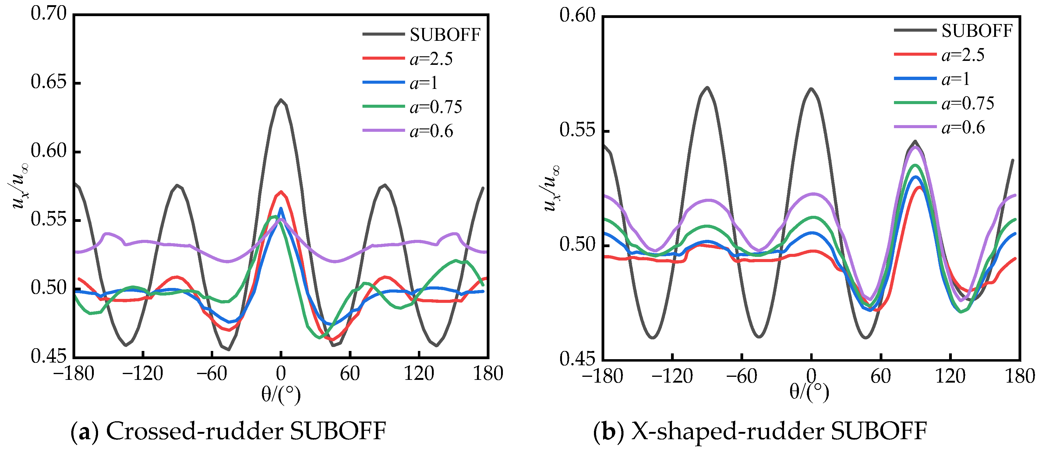
Larger fillets enhance the suppression of the horseshoe vortex, leading to improved velocity field homogeneity across the submarine propeller plane. Specifically, the circumferential velocity peak-to-valley difference at the propeller plane is reduced by 25.20% to 49.34%, highlighting the critical role of fillets in flow stabilization.

(5)

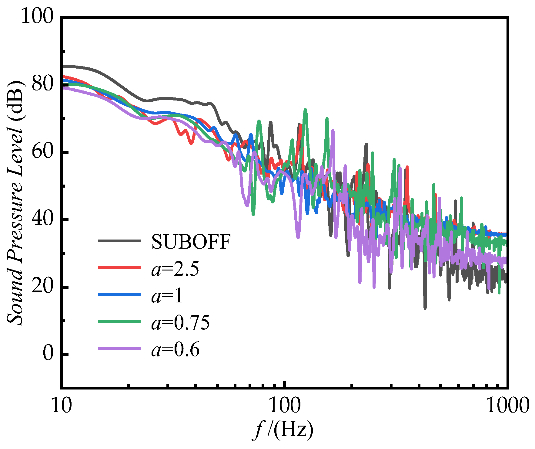
For the crossed rudder and “X” rudder, the addition of a fillet at their leading edges can achieve the effect of noise reduction. Respectively, the submarine hydrodynamic noise can be reduced by up to 4.6 dB and 5.6 dB.

References

1. Xiao, X.; Liang, Q.; Ke, L.; Hu, Y.; Zhang, L. Effects of X Rudder Area on the Horizontal Mechanical Properties and Wake Flow Field of Submarines. J. Phys. Conf. Ser. 2021, 2095, 012089. [Google Scholar] [CrossRef]
2. Zhou, G.L.; Ou, Y.P.; Gao, X.P.; Liu, R.J. Submarine Maneuverability Prediction Research Status and Prospects. Shipbuild. China 2018, 59, 203–214. [Google Scholar]
3. Cao, Z.J.; Xiao, C.R.; Li, S.Q.; Liang, Q.F. Comparative Stability Analysis of “X” Rudder and Crossed Rudder Submarines. Ship Sci. Technol. 2021, 43, 51–55. [Google Scholar]
4. Jiao, Y.C. Layout optimization of submarine X rudder. J. Ordnance Equip. Eng. 2018, 39, 40–44+71. [Google Scholar]
5. Toxopeus, S.; Kuin, R.; Kerkvliet, M.; Hoeijmakers, H.; Nienhuis, B. Improvement of resistance and wake field of an underwater vehicle by optimising the fin-body junction flow with CFD. In Proceedings of the ASME 2014 33rd International Conference on Ocean, Offshore and Arctic Engineering, San Francisco, CA, USA, 8–13 June 2014; American Society of Mechanical Engineers: New York, NY, USA, 2014. [Google Scholar]
6. Yeo, S.-J.; Hong, S.-Y.; Song, J.-H.; Seol, H.-S. Analysis of the effect of vortex reduction structures on submarine tonal noise via frequency-domain method employing thickness noise source. Ocean Eng. 2022, 257, 111640. [Google Scholar] [CrossRef]
7. Rahmani, M.; Gavzan, I.J.; Manshadi, M.D. Experimental investigation of the effect of sail geometry on the flow around the SUBOFF submarine model inspired by the dolphin’s dorsal fin. Ships Offshore Struct. 2023, 19, 769–778. [Google Scholar] [CrossRef]
8. Wang, X.; Huang, Q.; Pan, G. Numerical research on the influence of sail leading edge shapes on the hydrodynamic noise of a submarine. Appl. Ocean Res. 2021, 117, 102935. [Google Scholar] [CrossRef]
9. Li, M.J.; Wang, M.X.; Wang, L.; Liu, Z.H. Numerical simulation and experimental study of noise-reducing stern fillets of underwater navigational body. J. Ship Mech. 2016, 20, 1345–1354. [Google Scholar]
10. Jin, Z.; Wang, P.; Xia, H.; Ding, Y.; Han, P. Validation of Numerical Simulation on the Flow Field of Submarine with Various Types of stern appendages. In Proceedings of the OCEANS 2018 MTS/IEEE Charleston, Charleston, SC, USA, 22–25 October 2018. [Google Scholar]
11. Dai, J.C. Characterization of Propeller Radiated Noise and Hydroelastic Vibration. Master’s Thesis, Dalian University of Technology, Dalian, China, 2022. [Google Scholar]
12. Alin, N.; Fureby, C.; Svennberg, U.; Sandberg, W.; Ramamurti, R.; Bensow, R. Eddy Simulation of the Transient Flow around a Submarine during Maneuver. In Proceedings of the 45th AIAA Aerospace Sciences Meeting, Reno, NV, USA, 8–11 January 2007; pp. 17082–17099. [Google Scholar]
13. Liu, Z.H.; Xiong, Y. Control of submarine horseshoe vortices by vortex-reducing rectifiers and its comparison with the effect of auxiliary wings. J. Ship Mech. 2011, 15, 1102–1109. [Google Scholar]
14. Muscari, R.; Di Mascio, A.; Verzicco, R. Modeling of vortex dynamics in the wake of a marine propeller. Comput. Fluids 2013, 73, 65–79. [Google Scholar] [CrossRef]
15. Chen, H.; Yuan, X.X.; Bi, L.; Hua, R.H.; Si, F.F.; Tang, Z.G. Separate flow simulation based on a hybrid RANS/LES approach. Acta Aeronaut. ET Astronaut. Sin. 2020, 41, 177–188. [Google Scholar]
16. Liu, J.H.; Li, G.H.; Wang, F.X. Tilt-transition state rotor-wing aerodynamic interference characteristics. Acta Aeronaut. Astronaut. Sin. 2022, 43, 208–219. [Google Scholar]
17. Groves, N.C.; Huang, T.T.; Chang, M.S. Geometric Characteristics of DARPA SUBOFF Models; David Taylor Research Center: Washington, DC, USA, 1989. [Google Scholar]
18. Panton, R.L. Incompressible Flow; Wiley: Hoboken, NJ, USA, 2013. [Google Scholar]
19. Wilcox, D.C. Turbulence Modeling for CFD; DCW Industries: La Canada, CA, USA, 1998. [Google Scholar]
20. Hinze, J.O. Turbulence; McGraw-Hill Publishing Co: New York, NY, USA, 1975. [Google Scholar]
21. Wilcox, D.C. Reassessment of the Scale-Determining Equation for Advanced Turbulence Models. AIAA J. 1988, 26, 1299–1310. [Google Scholar] [CrossRef]
22. Zhang, Z.S.; Cui, G.X.; Xu, C.X.; Huang, W.X. Turbulence Simulation and Theory; Tsinghua University Press: Beijing, China, 2017. [Google Scholar]
23. Spalart, P.R.; Deck, S.; Shur, M.L.; Squires, K.D.; Strelets, M.K.; Travin, A. A New Version of Detached-Eddy Simulation, Resistant to Ambiguous Grid Densities. Theor. Comput. Fluid Dyn. 2006, 20, 181–195. [Google Scholar] [CrossRef]
24. Shur, M.L.; Spalart, P.R.; Strelets, M.K.; Travin, A.K. A Hybrid RANS-LES Approach with Delayed DES and Wall-Modelled LES Capabilities. Int. J. Heat Fluid Flow 2008, 29, 1638–1649. [Google Scholar] [CrossRef]
25. Ffowcs Williams, J.E.; Hawkings, D.L. Sound Generation by Turbulence and Surfaces in Arbitrary Motion. Philos. Trans. R. Soc. A 1969, 264, 321–342. [Google Scholar]
26. Park, S. CFD Study of Submarine Hydrodynamics near the Free Surface in Snorkel Conditions. Water 2025, 17, 734. [Google Scholar] [CrossRef]
27. Lositaño, I.C.M.; Danao, L.A.M. Steady wind performance of a 5 kW three-bladed H-rotor Darrieus Vertical Axis Wind Turbine (VAWT) with cambered tubercle leading edge (TLE) blades. Energy 2019, 175, 278–291. [Google Scholar] [CrossRef]
28. Huang, T.; Liu, H.L. Measurement of flows over an axisymmetric body with various appendages in a wind tunnel: The DARPA SUBOFF experimental program. Fluid Dyn. 1994, 5, 321. [Google Scholar]
Figure 1. Schematic structure of the horseshoe vortex.
Jmse 13 00830 g001
Figure 2. The SUBOFF model.
Jmse 13 00830 g002aJmse 13 00830 g002b
Figure 3. SUBOFF stern rudder parameters.
Jmse 13 00830 g003
Figure 4. The profile of the stern rudder with fillets.
Jmse 13 00830 g004aJmse 13 00830 g004b
Figure 5. Models of the stern rudder with fillets.
Jmse 13 00830 g005
Figure 6. Domain sensitivity analysis.
Jmse 13 00830 g006
Figure 7. Flow field computational domain.
Jmse 13 00830 g007
Figure 8. SUBOFF grids.
Jmse 13 00830 g008
Figure 9. SUBOFF wall y+.
Jmse 13 00830 g009
Figure 10. Cp along the upper meridian line [28].
Jmse 13 00830 g010
Figure 11. SUBOFF stern vortex distribution.
Jmse 13 00830 g011aJmse 13 00830 g011b
Figure 12. Comparison of forces between the crossed-rudder SUBOFF and the “X”-rudder SUBOFF.
Jmse 13 00830 g012
Figure 13. Speed distribution at the propeller plane.
Jmse 13 00830 g013
Figure 14. Comparison of the circumferential distributions of nondimensional axial velocity with and without fillets at r/R = 0.2.
Jmse 13 00830 g014
Figure 15. Spectrogram of the sound pressure levels of submarines with crossed rudders.
Jmse 13 00830 g015
Figure 16. Spectrogram of the sound pressure level of the “X”-rudder submarine.
Jmse 13 00830 g016
Figure 17. Comparison of the total sound pressure levels of crossed-rudder submarines.
Jmse 13 00830 g017
Figure 18. Comparison of the total sound pressure levels of “X”-rudder submarines.
Jmse 13 00830 g018