An Approach to Optimize the Efficiency of an Air Turbine of an Oscillating Water Column Based on Adaptive Model Predictive Control

Abstract

Wave energy, as a vast renewable resource, remains underutilized despite its high potential. The oscillating water column (OWC) is one of the most efficient way to harvest wave energy. Due to the randomness of ocean wave excitation, a control strategy is needed to keep the conversion efficiency of OWC at a certain level. In this paper, an adaptive model predictive control (AMPC) method is proposed to optimize the efficiency of the air turbine and improve the overall efficiency of the OWC. Experiments were conducted in a wave flume to obtain realistic wave data, which were fed into the AMPC model for simulations. Results indicate that AMPC-optimized turbine efficiency exhibits improved performance under regular wave conditions and significantly enhances efficiency within certain intervals under short-period irregular waves. However, as the wave period increases, optimization becomes less stable. Overall, the study concludes that the adaptive MPC model effectively optimizes turbine efficiency under most conditions, highlighting its potential for enhancing OWC performance.

1. Introduction

Wave resources are abundantly distributed worldwide, representing a vast reservoir of renewable energy [1]. Despite its high energy potential, wave energy, as a significant ocean energy source, remains underdeveloped and underutilized, with considerable untapped potential for exploitation [2]. Crucially, Wave Energy Converters (WECs) are pivotal in the development and harnessing of wave energy, functioning as the essential equipment for generating wave power [3].

The principle of wave power generation entails the use of WECs to capture wave energy [4,5]. This energy is then transmitted through mechanisms to convert it into relatively stable mechanical energy, which is ultimately transformed into electrical energy by generators. WECs are primarily categorized into three types: Oscillating Buoy (OB), Oscillating Water Column (OWC), and Overtopping (OT) [6,7,8,9]. Among these, OWC devices have garnered significant attention and application owing to their simple structure, low maintenance requirements, high durability, and excellent reliability. The increasing emergence of novel OWC designs further substantiates the feasibility of OWC-based wave energy conversion. So far, many OWC prototypes have been successfully developed, including Oceanlinx bottom-standing OWC, OE buoy, Oceanlinx greenWave [10] and Jida 4th (developed by the authors’ research team), as shown in Figure 1.

The air turbine serves as a pivotal component in the second and third stages of the OWC, exerting a direct influence on the overall performance and efficiency of the device. Among the various types of air turbines utilized in OWC systems, each exhibits distinct advantages and limitations. The impulse turbine, for instance, demonstrates superior peak efficiency; however, its intricate mechanical architecture imposes stringent manufacturing tolerances, thereby elevating production costs. In contrast, the Wells turbine has been widely adopted in OWC applications due to its structural simplicity, operational efficiency, and exceptional adaptability across varying flow conditions [11,12,13]. Furthermore, the Wells turbine’s symmetrical blade configuration endows it with self-rectifying properties, enabling it to operate efficiently in both forward and reverse flow directions. This symmetry in blade design also obviates the need for a complex direction control system, rendering it highly suitable for OWC devices powered by bidirectional airflow. Nevertheless, a drawback of the Wells turbine is that high efficiency is maintained only under specific external conditions. Recent studies have investigated the optimization of dual-radial impulse turbine designs to enhance their operational efficiency [14]. This research project will commence with an investigation into the Wells turbine, with the primary objective of employing control methodologies to enhance turbine efficiency, thereby improving the overall performance of the oscillating water column (OWC) system.

To address the issue of low efficiency in Oscillating Water Column (OWC) systems, an increasing number of control strategies have been applied, such as employing PID controllers to enhance power generation capacity [15], utilizing machine learning methods to reduce energy costs [16], adopting MPPT algorithms [17] and MPC control approaches to optimize output power, and implementing ET-BSC and ET-SMC algorithms to regulate turbine speed for improved energy utilization efficiency [18], Furthermore, control strategies have been implemented to optimize the wave-to-wire energy conversion process, thereby maximizing the efficiency of OWC systems [19]. Among these, Model Predictive Control (MPC) is particularly suitable for wave direction optimization studies due to its capability to solve optimal control sequences online and provide faster responses based on the system’s future dynamic behavior.

Model Predictive Control (MPC) represents an advanced control strategy that utilizes discretized mathematical models to compute all potential states in real time and ascertain the subsequent state that aligns with the optimal objective function, thereby attaining optimal control. In recent years, the application of MPC to wave energy converters has emerged as a new research trend [20,21,22,23]. For example, Li et al. [24,25] from Queen Mary University of London proposed an off-line linear non-causal control method based on the idea of model predictive control; Amann et al. [26] from the University of Stuttgart proposed the addition of an extended Kalman filter estimator to the model predictive control for a wave energy conversion device with two nonlinear point absorbers.; Milani et al. [27] of the Islamic Azad University of Iran, based on model pre-measurement control, proposed a method using a Kalman filter to observe state variables and predict the exciting force; Oetinger et al. [28] proposed decentralized and centralized control schemes for small-array wave energy converters based on MPC; Brekken [29] conducted MPC on WECs using their dynamic linear state space models. In terms of practical applications, Bracco et al. [30] of the Polytechnic University of Turin applied model predictive control to an inertial wave energy converter, while O ’Sullivan et al. [31] from University College Cork carried out model predictive control based on a model of the interaction between the array devices of the wave energy conversion device, and analyzed centralized and distributed model predictive control.

The inherently nonlinear nature of wave dynamics imposes significant limitations on conventional Model Predictive Control (MPC) when handling complex nonlinear system optimization. In contrast, the adaptive mechanism embedded in Adaptive Model Predictive Control (AMPC) demonstrates superior capability in solving optimization problems within such nonlinear complex systems. This intrinsic adaptability makes AMPC a more suitable control strategy for the present study. The principal novelty of this study resides in the innovative implementation of Adaptive Model Predictive Control (AMPC) for oscillating water column (OWC) wave energy converters. The proposed AMPC framework dynamically adapts to time-varying wave profiles by continuously optimizing system parameters through real-time predictive calculations. At each control interval, the algorithm computes an optimal solution that is subsequently fed back to the system model, enabling precise state adjustments and regulation of the pneumatic air flow rate within prescribed operational bounds. This control strategy significantly enhances the operational efficiency of Wells turbines in backward bent duct buoy (BBDB) configurations by maintaining optimal energy conversion conditions across varying wave regimes.

2. Principle of Adaptive Model Predictive Control

2.1. The Principle of Model Predictive Control

Model Predictive Control (MPC) is an advanced control strategy that uses a dynamic model of the system to predict future behavior and optimize control actions over a finite horizon. It solves an optimization problem at each time step to determine the best control inputs, considering constraints and objectives. Only the first control action is implemented, and the process repeats at the next time step, allowing for real-time adjustments. In addition, Model Predictive Control is a sophisticated control methodology that employs a mathematical model of the system to forecast its future behavior over a specified prediction horizon. At each control interval, MPC solves an optimization problem to determine a sequence of control actions that minimize a predefined cost function, which typically reflects desired performance criteria, such as tracking accuracy, energy efficiency, or other operational goals. This optimization takes into account various constraints, such as limits on control inputs, states, and outputs, ensuring that the system operates within safe and feasible bounds.

After solving the optimization problem, only the first control action in the sequence is applied to the system. The process is then repeated at the next time step with updated measurements, incorporating new information and disturbances. This rolling horizon approach allows MPC to adapt to changes and uncertainties in real time, making it highly effective for controlling complex, multivariable systems.

The principle of model predictive control can be explained by the following formula; assuming that we have a discrete dynamic time model, the discrete dynamic time model of the system is as follows:

$$x_{k+1}=A{x}_k+B{u}_k$$

(1)

where $x_{k+1}$ is the system state at time k, $u_k$ is the control input at time k, and A and B are system matrices. For the next N control horizons, the system state can be predicted as

$$x_{k+i|k}=A^i{x}_k+\sum _{j=0}^{i-1} A^{i-j-1}B{u}_{k+j|k}, i\in \left\{1,\dots ,N\right\}$$

(2)

where $x_{k+i|k}$ is the system state predicted i steps ahead based on the current time k.

The optimization objective of MPC is expressed as

$$J=\sum _{i=0}^{N_p-1} (x_{k+i|k}-x_{ref,k+i}{)}^{T}Q(x_{k+i|k}-x_{ref,k+i})+\sum _{i=0}^{N_e-1} u_{k+i|k}^{T}R{u}_{k+i|k}$$

(3)

where Q and R are weight matrices, $x_{ref,k+i}$ is the reference trajectory or setpoint at time $k+i$, $N_p$ is the prediction horizon length, and $N_c$ is the control horizon length.

The optimization problem can be seen as the process of finding the optimal control sequence. $u_{k|k},u_{k+1|k},\dots ,u_{k+N_c-1|k}$.

Therefore, the minimize cost function is formulated as

$$\begin{array}{c}\begin{array}{c}{x}_{k+i|k}=A^i{x}_k+\sum _{j=0}^{i-1} A^{i-j-1}B{u}_{k+j|k}\\ J_{min}=\mathit{min}\left(J_u,u\in \left\{u_{k|k},u_{k+1|k},\dots ,u_{k+N_c-1|k}\right\}\right)\end{array}\end{array}$$

(4)

To improve the convergence of the model, constraint conditions are introduced:

$$\begin{array}{c}\begin{array}{c}{u}_{min}\le u_{k+i|k}\le u_{max},i\in \left\{0,\dots ,N_c-1\right\}\\ x_{min}\le x_{k+i|k}\le x_{max},i\in \left\{1,\dots ,N_p-1\right\}\end{array}\end{array}$$

(5)

where $u_{min}$ and $u_{max}$ are the constraints on the control input, and $x_{min}$ and $x_{max}$ are the constraints on the state variables.

2.2. The Proposed Adaptive Model Predict Control for BBDB OWC

The schematic diagram of the Adaptive MPC turbine efficiency optimization model is shown in Figure 2. An external parameter (wave excitation force) is input into the control state space model, while another external parameter is input into the control device model to obtain the current Wells air turbine efficiency y_mo and the current state variable x. The AMPC calculates the ideal control output u_mv based on the current efficiency y_mo and the state space model and then feeds the control output back to the state space model and the control model for feedback correction. This completes the full process of efficiency control optimization.

3. The Construction of the Control State Space Model

3.1. Principle of the Control System

The simplified model diagram of the built efficiency control device is shown in Figure 3. When the wave hits the OWC buoy, the buoy will pitch around the center position. Consequently, the wave at the water inlet will rise and fall in the water column of the back bend, generating airflow. The control system then regulates the cross-sectional area of the air flow, resulting in control of the air turbine.

The correlation curve between the mass flow rate of the air turbine and turbine efficiency is shown in Figure 4 [14]. It can be observed that the turbine efficiency does not increase with the higher flow rate passing through the turbine. On the contrary, the turbine efficiency can only reach higher values within a specific flow rate range. In this paper, based on this principle, a control device is designed to control the mass flow rate passing through the turbine, thereby optimizing turbine efficiency, and the control device model is built based on this.

3.2. Parameter Analysis of the Control Device

Under the action of the external input torque and rotational damping shaft, the dynamic equation for the control device rotating counterclockwise around the shaft can be expressed as

$$T_{input}-T_f=J_{con}{\displaystyle \frac{d^2\theta }{d{t}^2}}$$

(6)

$$J_{con}={\int }_{-{\displaystyle \frac{L}{2}}}^{{\displaystyle \frac{L}{2}}} \rho hL\left({\displaystyle \frac{1}{12}}{L}^2+x^2\right)dx={\displaystyle \frac{1}{6}}m{L}^2$$

(7)

$$T_f=f{w}_{con}$$

(8)

where $T_{input}$ is the torque applied to the rotating shaft from the outside; $T_f$ is the reverse torque applied by the rotational damping shaft; $J_{con}$ is the moment of inertia of the rotating part; $\theta$ is the rotation angle (0° is the starting angle in the horizontal direction); $L$ indicates the length and width of the control device baffle facing the airflow direction; $\rho$ is the density of the control device baffle; $h$ is the height of the control device baffle; $m$ is the mass of the control device baffle; and $f$ is the damping coefficient of the rotational damping shaft.

Since the resultant force generated by the incident airflow in the pipeline acts along the axial direction, it does not produce a torque on the control device. Therefore, when analyzing the forces on this system, the moment effect of the incident airflow on the control device can be ignored.

3.3. Parameter Analysis of the Air Turbine

For large Reynolds numbers $\mathrm{R}\mathrm{e}>{10}^6$ and low Mach numbers $\mathrm{M}\mathrm{a}<0.3$, the performance characteristics of air turbines can be expressed in non-dimensional form as shown in the figure. The efficiency of air turbines can be expressed as a non-dimensional coefficient [19]:

$${\eta }_{\mathrm{t}\mathrm{u}\mathrm{r}\mathrm{b}}={\displaystyle \frac{P_{\mathrm{t}\mathrm{u}\mathrm{r}\mathrm{b}}}{P_{\mathrm{p}\mathrm{n}\mathrm{e}\mathrm{u}}}}={\displaystyle \frac{\mathsf{\Pi }}{\mathsf{\Phi }\mathsf{\Psi }}}={\displaystyle \frac{f_{\mathsf{\Pi }}\left(\mathsf{\Psi }\right)}{f_{\mathsf{\Phi }}\left(\mathsf{\Psi }\right)\mathsf{\Psi }}}$$

(9)

where

$$\begin{array}{c}\Phi =f_{\mathsf{\Phi }}\left(\mathsf{\Psi }\right), \Pi =f_{\mathsf{\Pi }}\left(\mathsf{\Psi }\right)\\ \Psi ={\displaystyle \frac{\Delta p}{{\rho }_{\mathrm{i}\mathrm{n}}{\mathrm{n}}^2{D}^2}}\\ \Phi ={\displaystyle \frac{q_{\mathrm{m}}}{{\rho }_{\mathrm{i}\mathrm{n}}\mathrm{n}{D}^3}}\\ \Pi ={\displaystyle \frac{P_{\mathrm{t}\mathrm{u}\mathrm{r}\mathrm{b}}}{{\rho }_{\mathrm{i}\mathrm{n}}{\mathrm{n}}^3{D}^5}}\end{array}$$

(10)

where $P_{\mathrm{p}\mathrm{n}\mathrm{e}\mathrm{u}}\mathsf{\Psi }$ is the non-dimensional pressure coefficient, $\mathsf{\Phi }$ is the non-dimensional air flow coefficient, $\mathsf{\Pi }$ is the non-dimensional turbine power coefficient, $q_{\mathrm{m}}$ is the mass flow rate of air in the turbine, $\Delta p$ is the pressure difference between the turbine inlet and outlet, ${\rho }_{\mathrm{i}\mathrm{n}}$ is the air density in the turbine cavity, n is the rotational speed of the air turbine, and D is the diameter of the rotor. The performance curve of the Wells turbine is shown in Figure 5.

The evaluation formula for the energy conversion efficiency of air turbines can also be expressed as

$$\eta ={\displaystyle \frac{w_{turb}{T}_{turb}}{v_{air}\Delta pS}}={\displaystyle \frac{w_{turb}{T}_{turb}}{v_{air}\Delta p{L}^2\left(1-\sin \theta \right)}}$$

(11)

where $w_{turb}$ is the angular velocity of the air turbine; $T_{turb}$ is the torque of the air turbine; $v_{air}$ is the flow velocity of the incident airflow; and $\Delta p$ is the pressure difference between the inlet and outlet of the air turbine.

Under the assumption of incompressible airflow conditions, the incident flow velocity can be analytically determined through the hydrodynamic free surface elevation data acquired by the wave gauge.

At different rotation angles, the cross-sectional area of air flowing through can be expressed as

$$S=L^2\left(1-\sin \theta \right)$$

(12)

where $S$ is the cross-sectional area of air flowing through; $L$ is the length of motion model; and $\theta$ is the rotation angle.

Assuming that the thickness of the baffle is very thin, it can be approximately ignored. When the baffle is rotated 180 degrees from the initial position (parallel to the turbine), the cross-sectional area of the air flow at this time is the cross-sectional area of the backbend.

The dynamic equation of the air turbine can be expressed as [32]

$$\begin{array}{c}{\displaystyle \frac{d}{dt}}\left({\displaystyle \frac{1}{2}}I{n}^2\right)=P_{turb}-P_{ctrl}=T_{turb}n-P_{ctrl}\\ P_{\mathrm{c}\mathrm{t}\mathrm{r}\mathrm{l}}=a_{\mathrm{b}\mathrm{e}\mathrm{p}}{n}^3\end{array}$$

(13)

where $I$ is the rotational inertia of the air turbine; $n$ is the rotational speed of the air turbine; $P_{turb}$ is the instantaneous turbine aerodynamic power (the product of the dynamic torque on the rotor and the rotational speed); $P_{ctrl}$ is the instantaneous generator power controlling the rotational speed; and $a_{\mathrm{b}\mathrm{e}\mathrm{p}}$ is an almost constant value.

4. Construction of Control Models

4.1. Linearization of Nonlinear Models

Since there is a nonlinear relationship between the state variables and control variables in the system model, the system cannot be represented in the form of a state space equation, which increases the difficulty of the solution. Therefore, the nonlinear system needs to be approximated or linearized to facilitate the obtaining of the required predicted state variables.

Let the target state variable be $x=[\theta w_{con}{]}^T$, and the control vector be $u=[T_{input}{]}^T$. The linearization process of the nonlinear system is actually the process of representing the above dynamic equations using a state space equation. Assuming that the control model operates at a small angle, the nonlinear model is approximately linearized through Taylor expansion in the vicinity of the operating point, ignoring higher-order infinitesimal terms. Then, Equation (11) can be expressed as

$$\eta ={\displaystyle \frac{w_{turb}{T}_{turb}}{v_{air}\Delta p{L}^2}}\left(1+\theta \right)$$

(14)

Rewrite the equation in the following form:

$$\left\{\begin{array}{c}{\displaystyle \frac{d\theta }{dt}}=w_{con}\hfill \\ {\displaystyle \frac{dw}{dt}}={\displaystyle \frac{f}{J_{con}}}\cdot w_{con}+{\displaystyle \frac{T_{input}}{J_{con}}}\hspace{0.25em}\hspace{0.25em}\hspace{0.25em}\hspace{0.25em}\end{array}\right.\Rightarrow \left[\begin{array}{c}\dot{\theta }\\ \dot{w}\end{array}\right]=\left[\begin{array}{cc}0& 1\\ 0& {\displaystyle \frac{f}{J_{con}}}\end{array}\right]\left[\begin{array}{c}\theta \\ w\end{array}\right]+\left[\begin{array}{c}0\\ {\displaystyle \frac{1}{J_{con}}}\end{array}\right]\left[T_{input}\right]$$

(15)

$$y=\left[{\displaystyle \frac{w_{turb}{T}_{turb}}{v_{air}\Delta p{L}^2}} 0\right]\left[\begin{array}{c}\theta \\ w\end{array}\right]+E$$

(16)

where $E$ and ${\displaystyle \frac{w_{turb}{T}_{turb}}{v_{air}\Delta p{L}^2}}$ are constants.

4.2. Discretization of Linear Models

Since the MPC algorithm requires a discrete-time state space model, it is necessary to discretize the above continuous-time state space model using a zero-order holder to obtain the following state space model:

$$\begin{array}{c}\dot{x}\left(k+1\right)=A_{d}x\left(k\right)+B_{d}u\left(k\right)\\ y\left(k\right)=C_{d}x\left(k\right)+D_{d}u\left(k\right)\end{array}$$

(17)

The relationship between the discrete model and the linear model is as follows:

$$\begin{array}{c}{A}_d=e^{A_C{T}_S}\\ B_d={\int }_0^{T_s} e^{A_C\tau }{B}_{c}d\tau \\ C_d=C_c\\ D_d=D_c\end{array}$$

(18)

where $A_d$ and $B_d$ are the discretized state matrix and input matrix, respectively, NS $C_d$ and $D_d$ are the output matrix and direct transfer matrix of the system, respectively. $T_S$ is the sampling time.

4.3. Predictive Model

Let the prediction horizon length BE $N_p$, then the system output prediction equation can be obtained based on Equation [33]:

$$X\left(k\right)=Z_{x}x\left(k\right)+Z_{u}u$$

(19)

where

$$X\left(k\right)=\left[\begin{array}{c}x\left(k\right)\\ x\left(k+1∣k\right)\\ ⋮\\ x\left(k+N_p-1∣k\right)\end{array}\right]$$

(20)

$$u=\left[\begin{array}{c}u\left(k\right)\\ u\left(k+1\right)\\ ⋮\\ u\left(k+N_p-1\right)\end{array}\right]$$

(21)

$$Z_x=\left[\begin{array}{c}{C}_d\\ {C_{d}A}_d\\ ⋮\\ {C_{d}A}_d^{N_p-1}\end{array}\right]$$

(22)

$$Z_u=\left[\begin{array}{ccccc}0& & & & \\ C_d{B}_{ud}& 0& & & \\ {C_{d}A}_d{B}_{ud}& {C_{d}B}_{ud}& 0& & \\ ⋮& ⋮& \ddots & \ddots & \\ {C_{d}A}_d^{N_p-2}{B}_{ud}& {C_{d}A}_d^{N_p-3}{B}_{ud}& \cdots & C_d{B}_{ud}& 0\end{array}\right]$$

(23)

The order of $X\left(k\right),$ $u$, $Z_x$ is ${2N}_p\times 1$, and the order of $Z_u$ is ${2N}_p\times N_p$.

Since the damping provided by the rotational damping shaft is limited, if the flow velocity of the incident airflow reaches a certain value, the device may not operate stably after rotating to the expected angle. Therefore, it is necessary to add system constraints on the operating conditions of the device. The air flow velocity needs to satisfy the following equation:

$$\left|v_{air}\right|<v_{max}$$

(24)

where $v_{max}$ is the maximum flow velocity that the device can withstand.

Meanwhile, in terms of efficiency optimization, it is necessary to keep the turbine within a stable and relatively efficient efficiency range. Therefore, system constraints need to be added to the output efficiency of the air turbine. The air turbine efficiency needs to satisfy the following equation:

$${\eta }_{min}<{\eta }_{turb}<{\eta }_{max}$$

(25)

where ${\eta }_{max}$ and ${\eta }_{min}$ are the upper and lower limits of the ideal efficiency, respectively.

5. Simulation Results and Analysis

5.1. Experimental Conditions

To better reference the working conditions of the model under real sea states, relevant flume experiments will be conducted on the model to obtain more realistic wave data. The wave-making flume used in the experiment is 30 m long, 1.2 m wide, and 0.55 m deep. By inputting relevant parameters through the wave-making machine control software on the PC as shown in the figure, expected period, wave height, regular or irregular waves can be generated.

The experimental model adopted is an oscillating water column (OWC) with a backward-bent tube. As shown in Figure 6, the device is approximately 0.875 m long, 0.462 m wide, 0.4 m high, and the cross-section of the backward-bent tube is square with a width of approximately 0.15 m [34].

The experiment was conducted under two wave conditions, regular waves and irregular waves, with wave periods of 0.9, 1.1, 1.3 s and 1.0, 1.5, 2.0 s, respectively. A sampling frequency of 50 Hz was employed, and the significant wave height was set at 3 cm. The specific experimental conditions are summarized in

Table 1. Experimental Operating Conditions.

Wave Form	Cycle	Sampling Frequency	Wave Height
Regular wave	$T_{1,2,3}=0.9,1.1, 1.3 \mathrm{s}$	$f=50 \mathrm{H}\mathrm{z}$	$H_{wave}=3 \mathrm{c}\mathrm{m}$
Irregular wave	$T_{4,5,6}=1.0,1.5, 2.0 \mathrm{s}$	$f=50 \mathrm{H}\mathrm{z}$	$H_{wave}=3 \mathrm{c}\mathrm{m}$

.

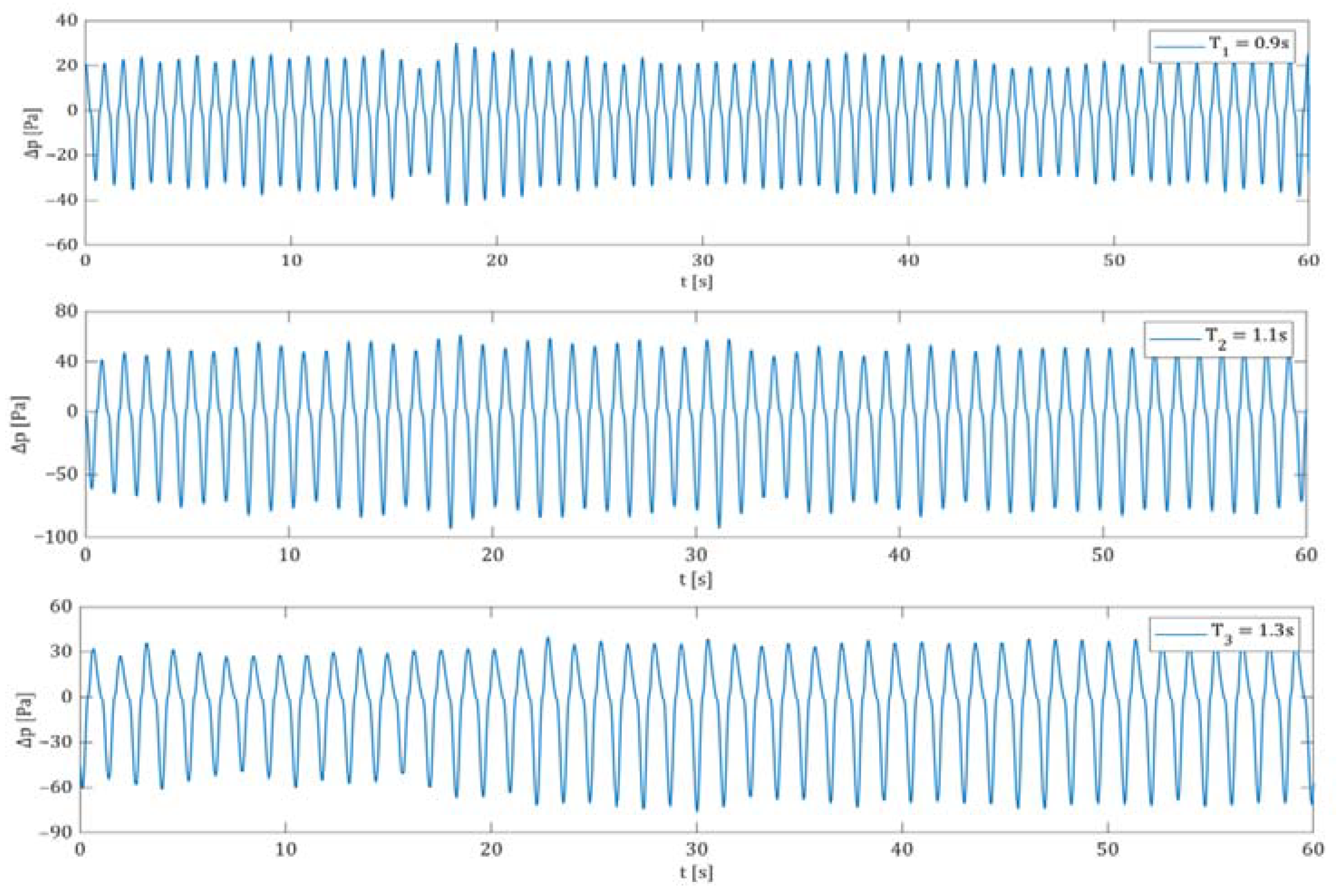
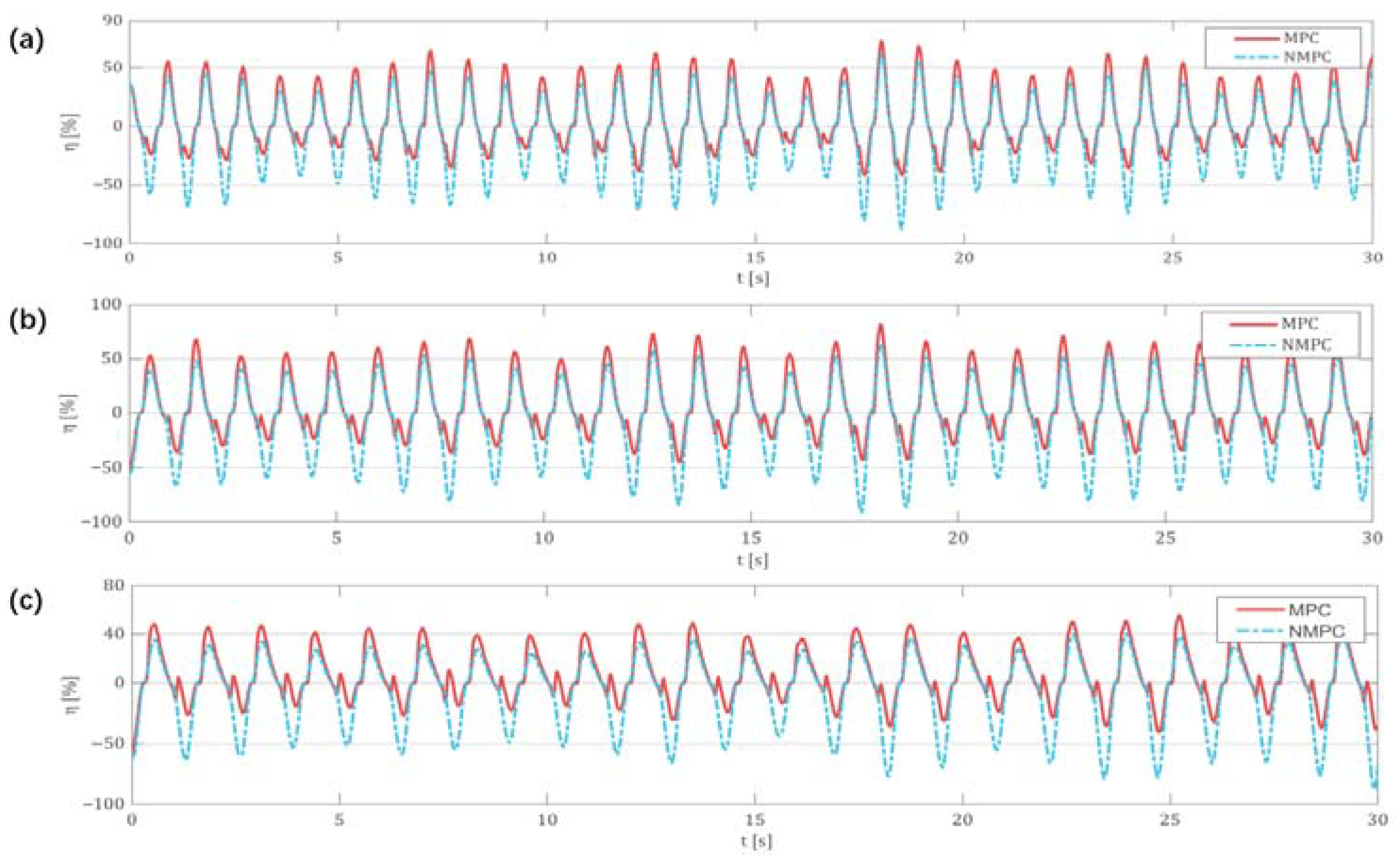
5.2. Simulation Results of Regular Wave Conditions

The external input of the system is set as the wave excitation force, from which the various external inputs required by the model are derived. Among them, the wave period for regular waves is set to $T_1=0.9 \mathrm{s};T_2=1.1 \mathrm{s};T_3=1.3 \mathrm{s}$ three cycles with three sets of data, the wave height is set as $H_{wave}=3 \mathrm{c}\mathrm{m}$, and the sampling frequency is set as $f=50 \mathrm{H}\mathrm{z}$. The pressure difference between the inlet and outlet of the turbine under regular waves for three cycles is shown in Figure 7:

In the Model Predictive Control (MPC) controller, the sampling time is set to 0.02 s, the prediction horizon is 20 s, and the control horizon is 3 s (the control horizon should be between 10 and 20% of the prediction horizon. A too-small control horizon may not achieve good control, while a larger control horizon may result in only the first part of the control horizon having useful effects. The reference efficiency is set to 80%, the upper limit constraint for turbine efficiency is 90%, and the upper limit for air flow velocity is 5 m/s. The pressure difference data from the above figure is imported into the MPC using an external module, and the corresponding cycle is set, yielding simulation results as shown in Figure 8.

From the MPC efficiency diagram for regular waves, it can be observed that, due to the bidirectional reciprocity of wave airflow within the backward-bent tube model, when the airflow reverses direction, the airflow velocity is opposite to the preset direction, resulting in negative efficiency values when calculated. However, since the Wells turbine has the characteristic of converting bidirectional airflow into unidirectional rotation, i.e., one-direction power generation, only the positive efficiency direction of the air turbine can be optimized, ignoring the negative efficiency of the air turbine.

It should be noted that the calculated turbine efficiency exhibits an overestimation due to unaccounted internal energy dissipation within the turbine assembly. Furthermore, hydrodynamic transfer losses occur as the wave excitation force propagates from the wavemaker to the test model, leading to attenuated energy delivery and consequent underestimation in performance quantification. In this study, both operating energy loss mechanisms (turbine dissipation and wave transmission attenuation) are assumed to occur in both conditions with or without AMPC, so it is neglected in the calculation efficiency calculations.

Within the positive efficiency range of the Wells air turbine, the MPC model exhibits good fitting with external excitation forces under regular wave conditions. Under wave conditions with three different periods, the optimization curves of the MPC for the air turbine are very similar. Under wave conditions with a short period of 1.3 s, after calculation, the average efficiency of the optimized turbine is about 63.1%, and the average efficiency of the unoptimized turbine is about 48.0%, an increase of 15.1%. Under a wave period of 1.1 s, the efficiency feedback from the Wells turbine is better, with an optimized average efficiency of approximately 58.7%; this is an increase of 16.2% compared to the non-optimized efficiency of 46.7%, and it can be well stabilized within this efficiency range. However, under wave conditions with longer period of 1.3 s, the turbine efficiency of the Wells turbine itself is in the low-efficiency range. After MPC optimization, the turbine efficiency fluctuates between 36.1% and 55.4% of the cycle, and the optimized efficiency of 45.2% is 14.0% higher than the non-optimized efficiency of 31.2%, indicating that the optimization of these three cycles by MPC can meet expected requirements. It also demonstrates that the adopted optimization strategy has high reliability and effectiveness in practical applications, contributing to enhancing the overall efficiency and economy of the system.

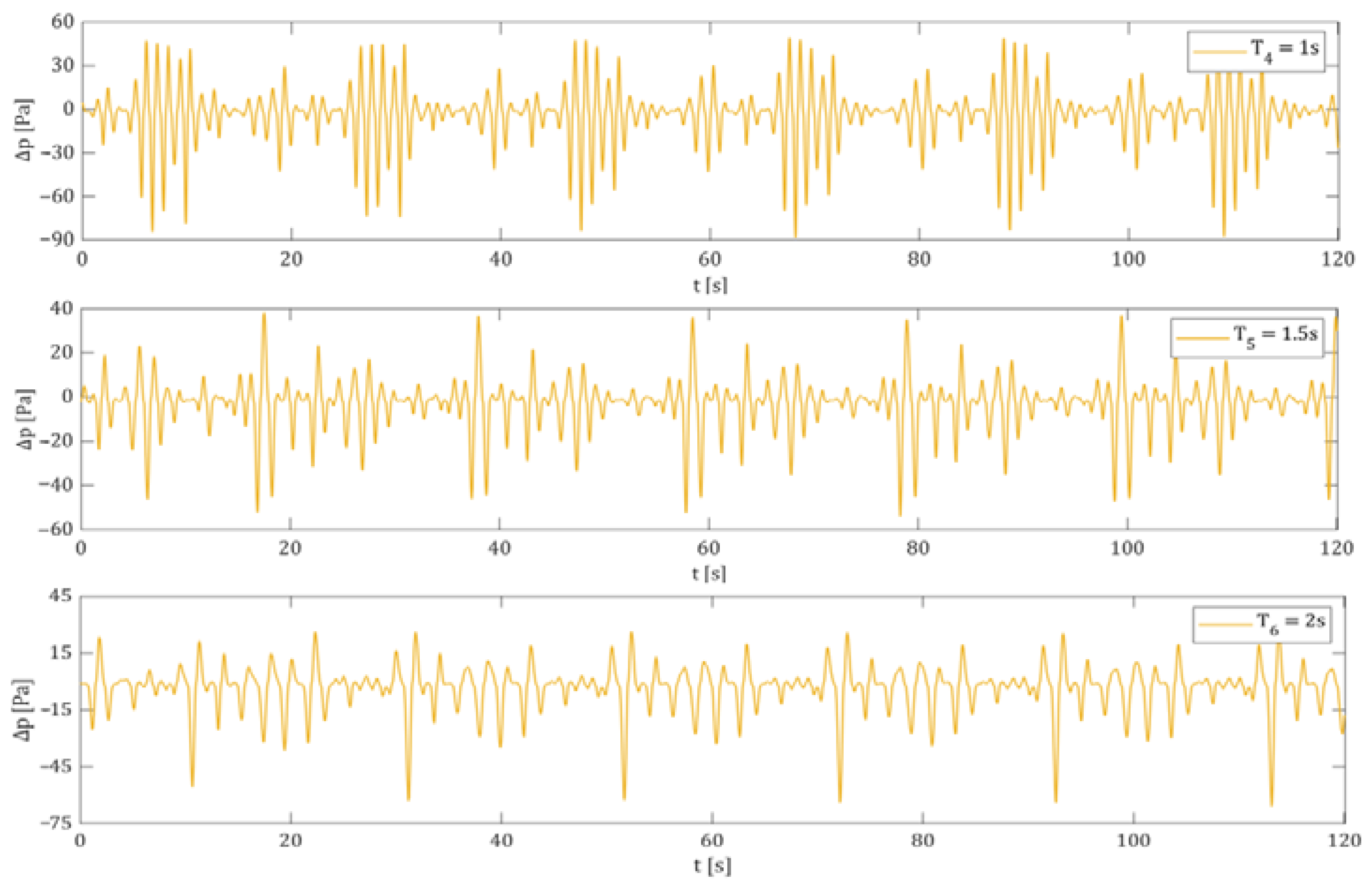
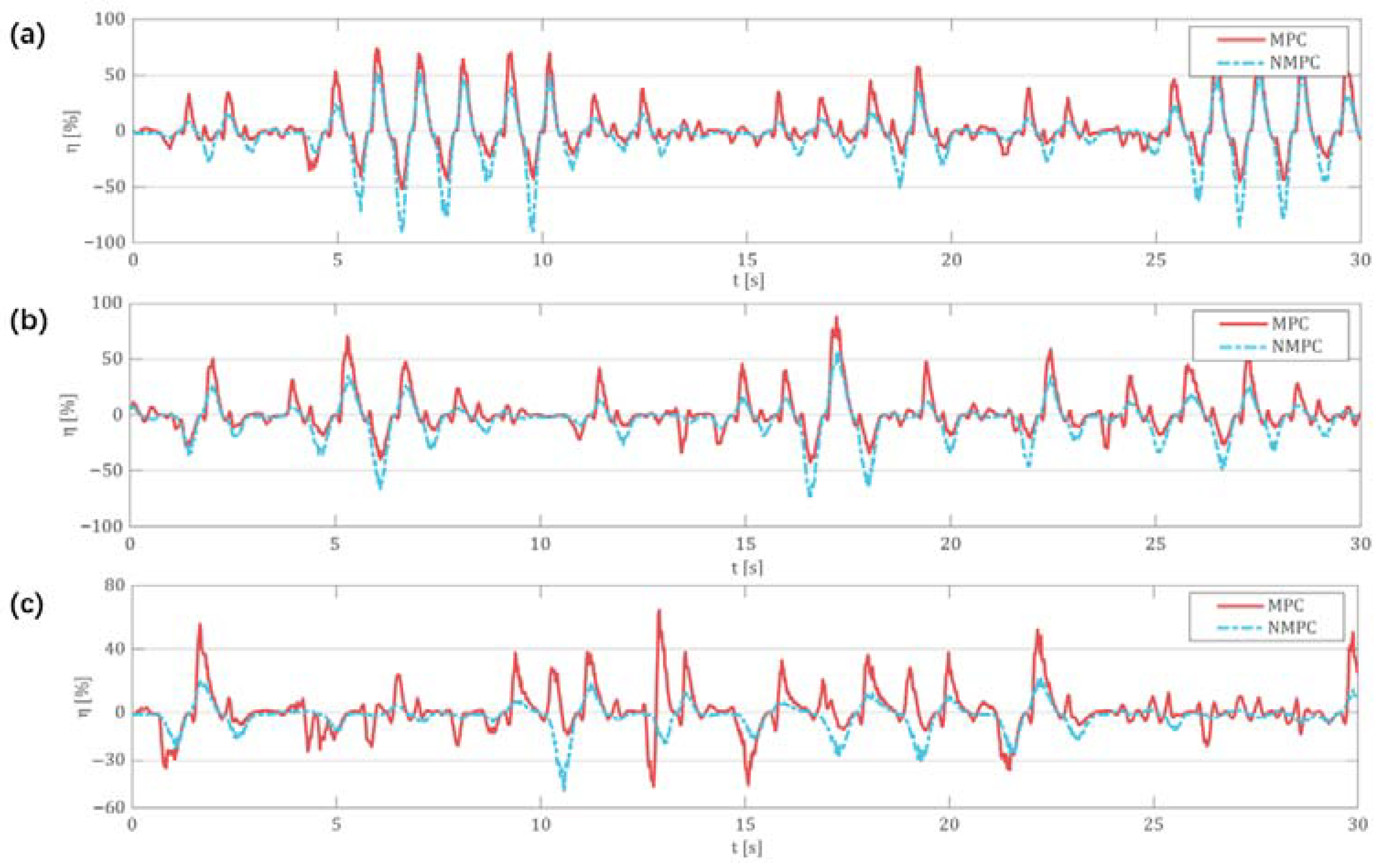
5.3. Simulation Results of Irregular Wave Conditions

The peak periods of the random wave spectrum are set as 1.0 s,1.5 s, and 2.0 s. The significant wave height is set as = 3 cm, and the sampling frequency is set as 50 Hz. The pressure difference between the inlet and outlet of the turbine in the backward-bent tube model under irregular waves for three cycles is shown in Figure 9.

The settings in the MPC controller for irregular waves are the same as those for regular waves: the sampling time is 0.02 s, the prediction horizon is 20 s, and the control horizon is 3 s. By setting the corresponding cycles, the simulation results are obtained as shown in Figure 10.

The figure illustrates the control efficiency predicted by the random wave model. In the region where the Wells air turbine efficiency is positive, when the period t = 1.0 s, due to the irregularity of random waves, the unoptimized efficiency of the Wells turbine remains low during the first 5 s. However, after optimization with AMPC, the efficiency sees a significant improvement, with an increase of approximately 19.8% compared to the unoptimized turbine efficiency. In the interval from 5 to 10 s, when the external excitation force reaches an appropriate level, the unoptimized Wells turbine efficiency peaks at 50.2%, falling within the medium efficiency range. Within this medium efficiency range, the MPC-optimized turbine efficiency reaches a maximum of 73.8%, belonging to the high efficiency range. This indicates that the MPC optimization method performs well in optimizing the turbine efficiency in both low and medium efficiency ranges under low-period wave conditions. Under random wave conditions, MPC can fit the unoptimized turbine efficiency curve relatively well, and the system’s response is relatively stable, which also demonstrates the excellent optimization performance of the MPC control method under low-period random wave conditions.

When the period t = 1.5 s, it can be observed that the turbine has strong responses at time points such as t = 5, 7, and 13 s. From 5 to 6 s, the efficiency increases from 33.9% to 69.8%. During these strong response intervals, the turbine exhibits different levels of high-efficiency optimization. At t = 17 to 18 s, the optimized maximum efficiency reaches 87.7%. It can be seen that, although the stability of MPC in turbine efficiency optimization is not as good as that in low-period conditions, its efficiency optimization in certain time intervals is significantly higher than that in low-period conditions during the same time intervals. However, under high-period wave conditions with t = 2 s, the efficiency optimization becomes unstable after 5 s, and this instability persists until the end of the simulation. This reflects that the MPC model’s ability to optimize the air turbine efficiency under high-period wave conditions with t = 2 s is relatively unstable and prone to instability. The observed instability may originate from the diminished flow velocity within the duct under high-cycle conditions, which reduces the turbine’s intrinsic efficiency. This creates a significant discrepancy between the actual turbine performance and the reference efficiency input to the AMPC model, making it challenging for the controller to converge toward the target optimization value. To mitigate this instability, the reference efficiency parameter in the AMPC model can be adaptively adjusted according to different wave cycle conditions. By reducing both the target efficiency and the expected turbine performance, the control system can achieve improved stability.

Figure 11 shows the torque required to be input into the control model under short-period regular and irregular wave conditions. Under regular wave conditions with a period of t = 0.9 s, the required input torque profile resembles the pressure difference diagram between the turbine inlet and outlet, with a maximum output torque of approximately 22 N·m. Under random wave conditions with a period of t = 1.0 s, the control torque reaches its maximum value of approximately 146.2 N·m at t = 23~24 s.

5.4. Discussion

The experimental results demonstrate that the AMPC model effectively enhances the turbine efficiency under both regular and irregular wave conditions. Specifically, under regular waves with periods of 0.9 s, 1.1 s, and 1.3 s, the turbine efficiency improved by 15.1%, 16.2%, and 14.0%, respectively. Under irregular waves with periods of 1.0 s, 1.5 s, and 2.0 s, the efficiency increased by 15.9%, 19.1%, and 21.5%, respectively. These results indicate that the AMPC model can improve the overall efficiency of the OWC system under both wave conditions.

However, the efficiency plots reveal that the AMPC model exhibits more stable optimization performance under regular waves, whereas its effectiveness under irregular waves is less consistent. Notably, as the wave period increases, the optimization instability becomes more pronounced, as evidenced by the significant variation in efficiency improvements (15.9% to 21.5%) across different irregular wave periods.

It should be noticed that the experiment in this study may still suffer from experimental errors:

(1)

AMPC model errors. These may arise from (i) the linearization of the original nonlinear model and (ii) discrepancies between predicted and actual outputs.

(2)

Control system errors in the physical model. The rotating damping shaft is prone to rust formation due to prolonged water exposure, leading to torque regulation inaccuracies.

(3)

Energy losses in the air turbine. These include losses due to air resistance and mechanical inefficiencies.

6. Conclusions

This paper designs a control device to enhance air turbine efficiency. By solving relevant equations and using the MPC optimization control method, simulations in Matlab/Simulink led to the following conclusions:

(1)

MPC-optimized turbine efficiency shows slight improvement in regular waves. Under wave periods of 0.9 s, 1.1 s and 1.3 s, the turbine efficiency is increased by 15.1%, 16.2% and 14.0% respectively.

(2)

MPC is effective for short-period irregular waves but becomes unstable as the wave period increases. The standard deviations of efficiency fluctuations under irregular wave conditions with periods of 1.5 s and 2.0 s were measured as 4.929 and 8.134, respectively.

(3)

The MPC adaptive model optimizes turbine efficiency under most conditions.

In future research, the control model will be improved for better optimization in both regular and irregular wave conditions, and a physical prototype of the control device will be conducted based on simulation feasibility. To address potential experimental discrepancies, comprehensive consideration will be given to errors arising from control models, actual system dynamics, and turbine energy losses. Moreover, after the optimization of considerations above, the proposed method will be applied in the real sea test prototype to testify its performance under more severe wave conditions for further validation.

References

1. Xu, J.; Li, J.; Pan, S.; Yao, Y.; Chen, L.; Wu, Z. Assessment of Wind and Wave Energy in China Seas under Climate Change Based on CMIP6 Climate Model. Energy 2024, 310, 133207. [Google Scholar] [CrossRef]
2. Yang, M.Y.; Shao, H.; Zhao, X.; Cheng, G.; Dai, S.; Wang, L.; Mao, X.Z. Spatiotemporal Distribution, Evolution, and Complementarity of Wind and Waves in China’s Offshore Waters and Its Implications for the Development of Green Energy. Energy Convers. Manag. 2024, 312, 118567. [Google Scholar] [CrossRef]
3. Wan, Y.; Zheng, C.; Li, L.; Dai, Y.; Esteban, M.D.; López-Gutiérrez, J.S.; Qu, X.; Zhang, X. Wave Energy Assessment Related to Wave Energy Convertors in the Coastal Waters of China. Energy 2020, 202, 117741. [Google Scholar] [CrossRef]
4. Jin, H.; Zhang, H.; Xu, D.; Jun, D.; Ze, S. Low-Frequency Energy Capture and Water Wave Attenuation of a Hybrid WEC-Breakwater with Nonlinear Stiffness. Renew. Energy 2022, 196, 1029–1047. [Google Scholar] [CrossRef]
5. Chow, Y.C.; Chang, Y.C.; Chen, D.W.; Lin, C.C.; Tzang, S.Y. Parametric Design Methodology for Maximizing Energy Capture of a Bottom-Hinged Flap-Type WEC with Medium Wave Resources. Renew. Energy 2018, 126, 605–616. [Google Scholar] [CrossRef]
6. Falnes, J. A Review of Wave-Energy Extraction. Mar. Struct. 2007, 20, 185–201. [Google Scholar] [CrossRef]
7. Falcão, A.F.d.O. Wave Energy Utilization: A Review of the Technologies. Renew. Sustain. Energy Rev. 2010, 14, 899–918. [Google Scholar] [CrossRef]
8. Jagath Kumara, K.D.R. A Top-Mounted, Chain-Driven, Bidirectional Point Absorber Type Wave Energy Convertor. Energy Rep. 2024, 12, 1360–1384. [Google Scholar] [CrossRef]
9. Cheng, Y.; Fu, L.; Dai, S.; Collu, M.; Cui, L.; Yuan, Z.; Incecik, A. Experimental and Numerical Analysis of a Hybrid WEC-Breakwater System Combining an Oscillating Water Column and an Oscillating Buoy. Renew. Sustain. Energy Rev. 2022, 169, 112909. [Google Scholar] [CrossRef]
10. Falcão, A.F.O.; Henriques, J.C.C. Oscillating-Water-Column Wave Energy Converters and Air Turbines: A Review. Renew. Energy 2016, 85, 1391–1424. [Google Scholar] [CrossRef]
11. Gratton, T.; Ghisu, T.; Parks, G.; Cambuli, F.; Puddu, P. Optimization of Blade Profiles for the Wells Turbine. Ocean Eng. 2018, 169, 202–214. [Google Scholar] [CrossRef]
12. Halder, P.; Rhee, S.H.; Samad, A. Numerical Optimization of Wells Turbine for Wave Energy Extraction. Int. J. Nav. Archit. Ocean Eng. 2017, 9, 11–24. [Google Scholar] [CrossRef]
13. Fenu, B.; Henriques, J.C.C.; Glorioso, M.; Gato, L.M.C.; Bonfanti, M. Real-Time Wells Turbine Simulation on an Oscillating-Water-Column Wave Energy Converter Physical Model. Appl. Energy 2024, 376, 124121. [Google Scholar] [CrossRef]
14. Elatife, K.; El Marjani, A. Design Optimization and Analysis of a Compact Twin Radial Impulse Turbine for Wave Energy Conversion. Results Eng. 2024, 24, 103561. [Google Scholar] [CrossRef]
15. M’zoughi, F.; Bouallègue, S.; Garrido, A.J.; Garrido, I.; Ayadi, M. Stalling-Free Control Strategies for Oscillating-Water-Column-Based Wave Power Generation Plants. IEEE Trans. Energy Convers. 2018, 33, 209–222. [Google Scholar] [CrossRef]
16. M’zoughi, F.; Lekube, J.; Garrido, A.J.; De La Sen, M.; Garrido, I. Machine Learning-Based Diagnosis in Wave Power Plants for Cost Reduction Using Real Measured Experimental Data: Mutriku Wave Power Plant. Ocean Eng. 2024, 293, 116619. [Google Scholar] [CrossRef]
17. Mishra, S.K.; Purwar, S.; Kishor, N. Maximizing Output Power in Oscillating Water Column Wave Power Plants: An Optimization Based MPPT Algorithm. Technologies 2018, 6, 15. [Google Scholar] [CrossRef]
18. Mishra, S.K.; Purwar, S.; Kishor, N. Event-Triggered Nonlinear Control of OWC Ocean Wave Energy Plant. IEEE Trans. Sustain. Energy 2018, 9, 1750–1760. [Google Scholar] [CrossRef]
19. Rosati, M.; Ringwood, J.V. Wave-to-Wire Efficiency Maximisation for Oscillating-Water-Column Systems. IFAC-Pap. 2023, 56, 10886–10891. [Google Scholar] [CrossRef]
20. Faedo, N.; Olaya, S.; Ringwood, J.V. Optimal Control, MPC and MPC-like Algorithms for Wave Energy Systems: An Overview. IFAC J. Syst. Control. 2017, 1, 37–56. [Google Scholar] [CrossRef]
21. Zhang, M.; Yu, S.R.; Zhao, G.W.; Dai, S.S.; He, F.; Yuan, Z.M. Model Predictive Control of Wave Energy Converters. Ocean Eng. 2024, 301, 117430. [Google Scholar] [CrossRef]
22. Li, D.; Wang, T.; Tao, J.; Sharma, S.; Borthwick, A.G.L.; Dong, X.; Shi, H. Model Predictive Control of a Single-Buoy Wave Energy Converter with Coupled Constraints and Model Adaptation. Ocean Eng. 2025, 315, 119887. [Google Scholar] [CrossRef]
23. Zhan, S.; Chen, Y.; Ringwood, J.V. Computationally-Efficient Nonlinear Model Predictive Control of Wave Energy Converters with Imperfect Wave Excitation Previews. Ocean Eng. 2025, 319, 120125. [Google Scholar] [CrossRef]
24. Liao, Z.; Gai, N.; Stansby, P.; Li, G. Linear Non-Causal Optimal Control of an Attenuator Type Wave Energy Converter M4. IEEE Trans. Sustain. Energy 2020, 11, 1278–1286. [Google Scholar] [CrossRef]
25. Zhan, S.; Li, G. Linear Optimal Noncausal Control of Wave Energy Converters. IEEE Trans. Control Syst. Technol. 2019, 27, 1526–1536. [Google Scholar] [CrossRef]
26. Amann, K.U.; Magaña, M.E.; Sawodny, O. Model Predictive Control of a Nonlinear 2-Body Point Absorber Wave Energy Converter With Estimated State Feedback. IEEE Trans. Sustain. Energy 2015, 6, 336–345. [Google Scholar] [CrossRef]
27. Milani, F.; Moghaddam, R.K. Power Maximization of a Point Absorber Wave Energy Converter Using Improved Model Predictive Control. China Ocean Eng. 2017, 31, 510–516. [Google Scholar] [CrossRef]
28. Oetinger, D.; Magana, M.E.; Sawodny, O. Decentralized Model Predictive Control for Wave Energy Converter Arrays. IEEE Trans. Sustain. Energy 2014, 5, 1099–1107. [Google Scholar] [CrossRef]
29. Ted, K.A. Brekken on Model Predictive Control for a Point Absorber Wave Energy Converter. In Proceedings of the 2011 IEEE PES Trondheim PowerTech: The Power of Technology for a Sustainable Society, NTNU, Trondheim, Norway, 19–23 June 2011; IEEE: Piscataway, NJ, USA, 2011. ISBN 9781424484171. [Google Scholar]
30. Bracco, G.; Canale, M.; Cerone, V. Energy harvesting optimization of an Inertial Sea Wave Energy Converter through Model Predictive Control. In Proceedings of the 2019 IEEE 15th International Conference on Control and Automation (ICCA), Edinburgh, Scotland, 16–19 July 2019; IEEE: Piscataway, NJ, USA, 2019. ISBN 9781728111643. [Google Scholar]
31. O’Sullivan, A.C.M.; Sheng, W.; Lightbody, G. An Analysis of the Potential Benefits of Centralised Predictive Control for Optimal Electrical Power Generation from Wave Energy Arrays. IEEE Trans. Sustain. Energy 2018, 9, 1761–1771. [Google Scholar] [CrossRef]
32. Henriques, J.C.C.; Portillo, J.C.C.; Sheng, W.; Gato, L.M.C.; Falcão, A.F.O. Dynamics and Control of Air Turbines in Oscillating-Water-Column Wave Energy Converters: Analyses and Case Study. Renew. Sustain. Energy Rev. 2019, 112, 571–589. [Google Scholar] [CrossRef]
33. Zhang, Z.; Qin, J.; Zhang, Y.; Huang, S.; Liu, Y.; Xue, G. Cooperative Model Predictive Control for Wave Energy Converter Arrays. Renew. Energy 2023, 219, 119441. [Google Scholar] [CrossRef]
34. Zhu, W.; Du, Z.; Tu, Y.; Huang, Y.; Liang, B.; Chen, X.; Cao, G.; Xiao, S.; Yang, S. Experimental Study of a Backward Bent Duct Buoy Wave Energy Converter: Effects of the Air Chamber and Center of Gravity Height. Ocean Eng. 2024, 313, 119447. [Google Scholar] [CrossRef]
Figure 1. OWC developed prototypes: (a) Oceanlinx bottom-standing OWC, (b) OE buoy, (c) Oceanlinx green Wave, (d) Jida 4th.
Jmse 13 00831 g001
Figure 2. Schematic diagram of proposed adaptive MPC for OWC turbine.
Jmse 13 00831 g002
Figure 3. Dynamic Model Diagram of Efficiency Control Device.
Jmse 13 00831 g003
Figure 4. Curve of turbine efficiency and mass flow rate.
Jmse 13 00831 g004
Figure 5. Relationship between Φ , Π , η t u r b , and Ψ Wells turbine.
Jmse 13 00831 g005
Figure 6. Experiment Details: (a) Wave-making Flume, (b) 3D Model of Backward-bent Tube, (c) Experimental prototype.
Jmse 13 00831 g006
Figure 7. Pressure Difference between Inlet and Outlet of Wells Turbine under Regular Wave Conditions.
Jmse 13 00831 g007
Figure 8. Optimized and Unoptimized Efficiency of Wells Turbine under Regular Wave Conditions: (a) T1 = 0.9 s, (b) T2 = 1.1 s, (c) T3 = 1.3 s.
Jmse 13 00831 g008
Figure 9. Pressure Difference between Inlet and Outlet of Wells Turbine under Irregular Wave Conditions.
Jmse 13 00831 g009
Figure 10. Optimized and Unoptimized Efficiency of Wells Turbine under Irregular Wave Conditions: (a) T4 = 1.0 s, (b) T5 = 1.5 s, (c) T6 = 2.0 s.
Jmse 13 00831 g010
Figure 11. Model Control Torque Input under Short-period Regular and Irregular Wave Conditions.
Jmse 13 00831 g011