Dynamic Reusable Workflows for Ocean Science

Abstract

Digital catalogs of ocean data have been available for decades, but advances in standardized services and software for catalog searches and data access now make it possible to create catalog-driven workflows that automate—end-to-end—data search, analysis, and visualization of data from multiple distributed sources. Further, these workflows may be shared, reused, and adapted with ease. Here we describe a workflow developed within the US Integrated Ocean Observing System (IOOS) which automates the skill assessment of water temperature forecasts from multiple ocean forecast models, allowing improved forecast products to be delivered for an open water swim event. A series of Jupyter Notebooks are used to capture and document the end-to-end workflow using a collection of Python tools that facilitate working with standardized catalog and data services. The workflow first searches a catalog of metadata using the Open Geospatial Consortium (OGC) Catalog Service for the Web (CSW), then accesses data service endpoints found in the metadata records using the OGC Sensor Observation Service (SOS) for in situ sensor data and OPeNDAP services for remotely-sensed and model data. Skill metrics are computed and time series comparisons of forecast model and observed data are displayed interactively, leveraging the capabilities of modern web browsers. The resulting workflow not only solves a challenging specific problem, but highlights the benefits of dynamic, reusable workflows in general. These workflows adapt as new data enter the data system, facilitate reproducible science, provide templates from which new scientific workflows can be developed, and encourage data providers to use standardized services. As applied to the ocean swim event, the workflow exposed problems with two of the ocean forecast products which led to improved regional forecasts once errors were corrected. While the example is specific, the approach is general, and we hope to see increased use of dynamic notebooks across geoscience domains.

1. Introduction

1.1. Motivation

When tackling a scientific or engineering problem that requires integrating information from a large number of data providers, a challenging issue can be simply finding and acquiring the data. While digital systems for cataloging scientific data have existed for decades (e.g., NASA GCMD [1] and GEOSS Portal [2]) these systems have typically been used to conduct geospatial, temporal, and keyword searches that return links to web sites or documents containing data in a variety of forms and formats, requiring significant work on the part of the would-be user to determine how to access, download, and decode the data they require.

However, with the increasing availability of standardized, varied, and powerful web-based data services, users can now employ catalog services to not only find data across multiple providers, but then to acquire these data in a programmatic way, so that both search and access are automated.

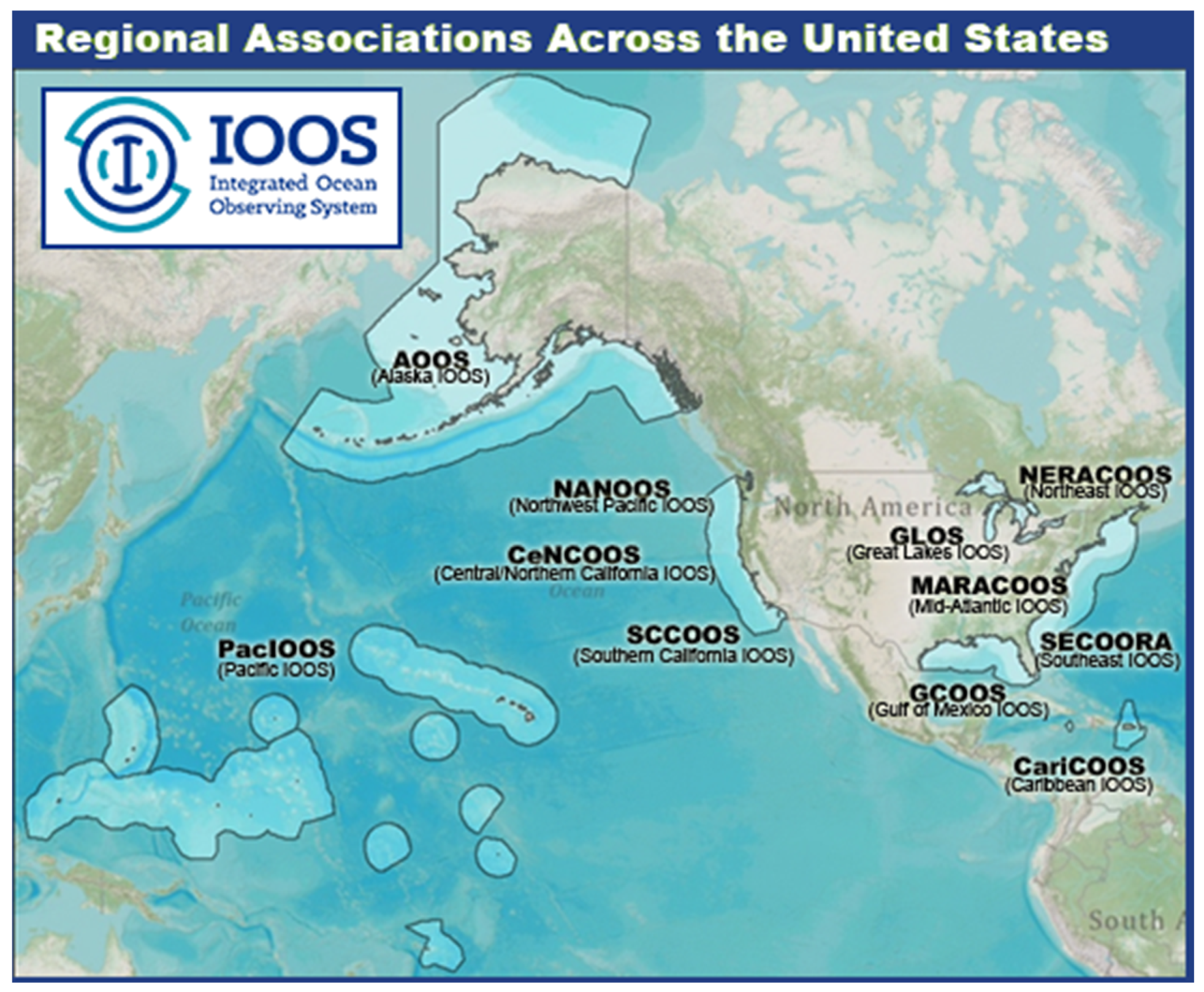
This approach is being supported by organizations worldwide (for example, the national catalogs data.gov, data.gov.uk, data.gov.au, geodata.gov.gr). Here we describe support and use within the US Integrated Ocean Observing system (IOOS) [3,4], a partnership between 17 federal agencies and 11 regional associations (Figure 1). IOOS partners use a wide range of different sensors and models, but are required to supply data using approved web services: for example, OGC-SOS [5] and/or ERDDAP [6] for sensor data, OPeNDAP [7] with CF-Conventions [8] for model data. They are also required to provide ISO 19115-2 metadata [9] for each dataset. The use of both standardized web services and standardized metadata enables a high degree of interoperability [10,11].

Demonstrating how to effectively use these catalogs and data services can be challenging. Fortunately, with the rise of interactive, scientific notebooks that use modern browsers as a client to communicate with back-end servers, end-to-end workflows for scientific data discovery, access, analysis, and visualization can be constructed that embed code, descriptions, and results into documents that can be shared, reused, and adapted by others [12].

We demonstrate here a specific application of this approach to assessing the predictive skills of water temperature forecasts from multiple ocean models within the US Integrated Ocean Observing System (US-IOOS).

1.2. The Boston Light Swim Problem

The Boston Light Swim (“Granddaddy of American Open Water Swims”) is an eight-mile swim that has been held every August since 1907. With a no-wet-suit requirement and water temperatures as low as 58 degrees F, swimmers are monitored carefully and pulled from the water if they do not make specified waypoints in required times (swimmers must finish the entire race within 5 h). Since water temperatures can fluctuate substantially with wind events, such as upwelling, race organizers are interested in forecast water temperatures so they can inform swimmers and their support teams of how hazardous conditions are likely to be.

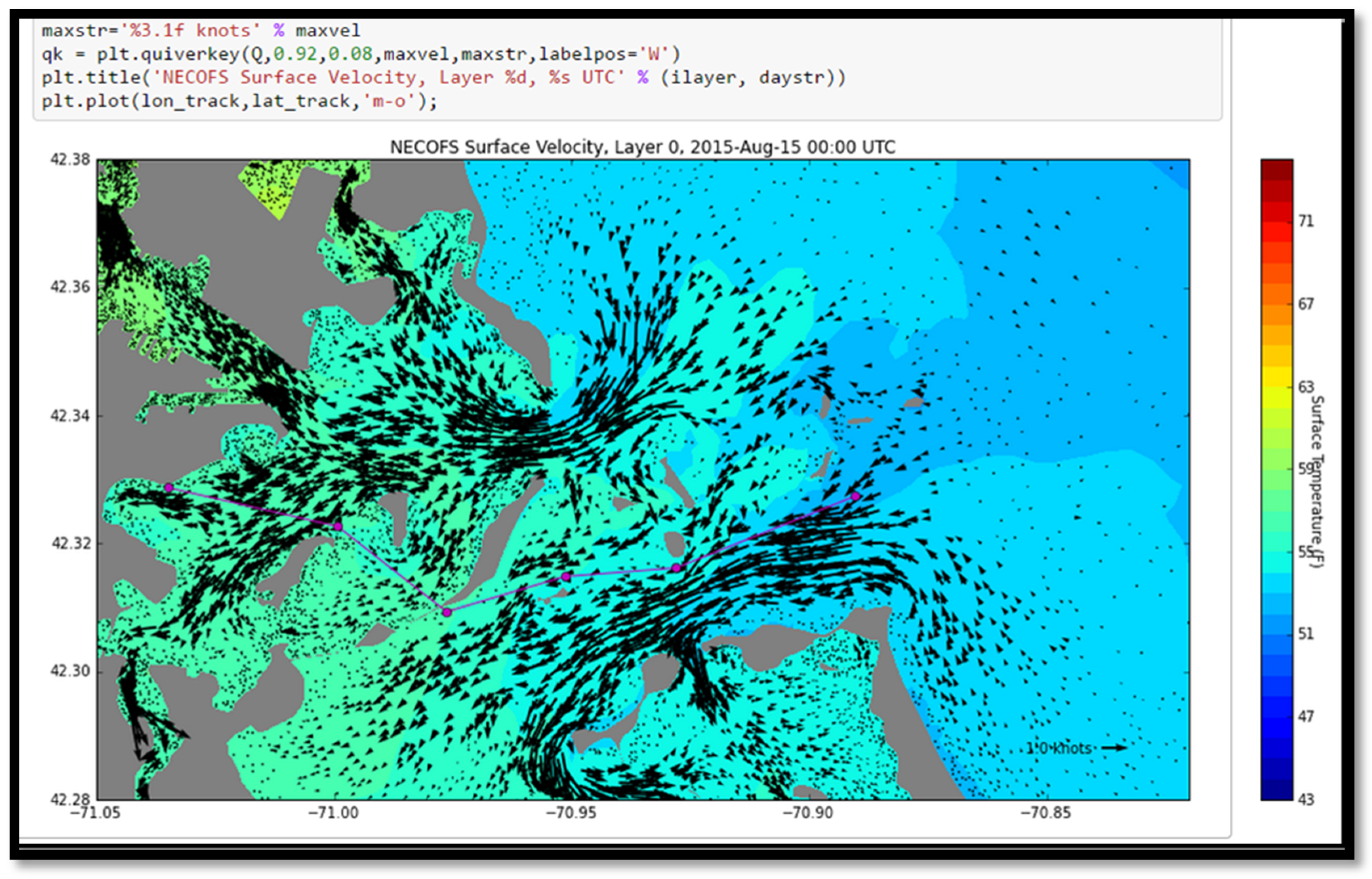
On 13 August 2015, two days before the race, swim organizers expressed concern that the highest-resolution IOOS forecast model was predicting very cold temperatures for race day (Figure 2) and they inquired about the degree they should believe the model. To address this issue, we realized we could simply reuse an existing workflow developed for the IOOS System Test [13], which automated the assessment of predicted water levels at coastal tide gauge locations. What if we just deployed the same notebook to assess the quality of predicted water temperatures, but changed the search criteria to look for water temperatures rather than water levels? This simple modification was successful and allowed us to respond to the swimmers’ issue with improved forecast products, demonstrating the power of the dynamic, reusable workflow approach.

2. Methods

2.1. Approach

We constructed the workflow as a series of Jupyter Notebooks (Supplementary Materials), web applications that combine live code, equations, visualizations, and explanatory text [14]. Although the workflow could have been constructed as a single notebook, we split the tasks into three notebooks to allow users to more easily re-run certain sections of the workflow. The first notebook performs queries on a catalog service (or services), then retrieves data using discovered data services and saves the results to disk. The second notebook loads the retrieved data and creates skill assessment products, writing those products to disk. The third notebook loads the products and displays them on an interactive map in the browser. In the following sections, we describe the components that make this workflow possible, and then describe the function of each notebook in more detail.

2.2. Standard Web Services

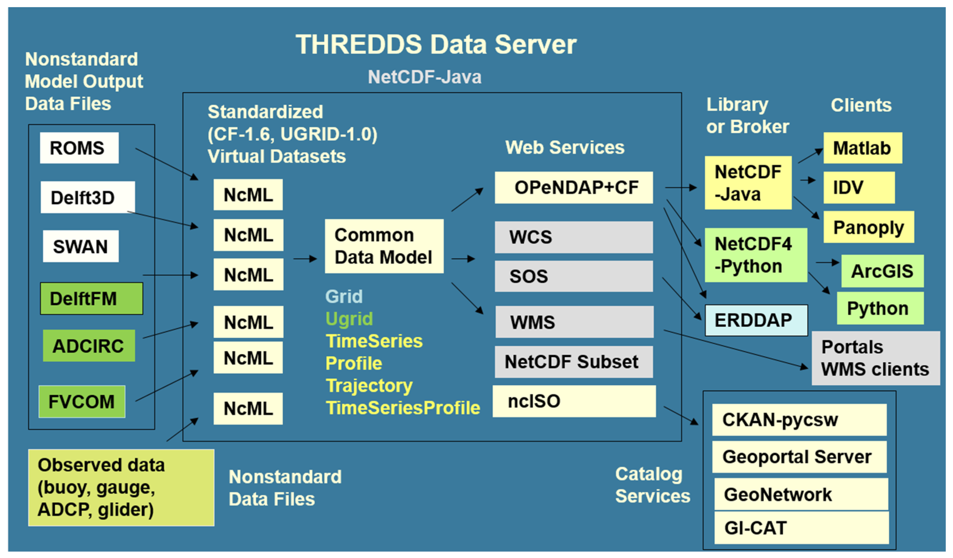
As previously mentioned, data providers in IOOS are required to provide web data services from an approved list of international and community standards. For sensor data, one of the most commonly-supported services is OGC-SOS and for model output, OPeNDAP with CF Conventions. These services are designed to allow time series and model output from diverse sensors and modeling systems to be treated in a common way, without model- or sensor-specific code required for access and use. Typically in IOOS these services are provided by the Unidata THREDDS Data Server (TDS) [15], free open-source software which allows collections of NetCDF [16] files to be virtually aggregated and supplemented with metadata via NcML [17] (Figure 3). For more information on the benefits of the TDS approach and how data providers can establish standard services, see [18,19,20,21,22].

In addition to requiring standardized data services, IOOS also requires that standardized ISO metadata (ISO 19115-2) be created for each dataset. This is easily generated using the ncISO software [23], which automatically converts attributes from NetCDF, NcML, and the TDS into ISO metadata documents. Each region of IOOS maintains a web-accessible folder of ISO metadata that is harvested daily into a centralized database, which can then be searched using a GUI or programmatically using the OGC-CSW service. These capabilities are provided by the free open-source CKAN [24] and pycsw [25] software packages.

With these services in place, we used a series of Jupyter Notebooks to (1) search and acquire data; (2) compute skill assessment metrics; and (3) show the skill assessment results on an interactive map. The Jupyter Notebooks combine the ability to document the workflow, show actual code used for search, access, analysis, and visualization, as well as the results, in a single reproducible document format. Although Jupyter Notebooks can be constructed using many languages, including MATLAB, R, and Julia, here we use Python due to the availability of packages that facilitate working with the web services used in IOOS.

2.3. Fetch Data Notebook

This notebook searches for data by querying a CSW service to extract metadata records from the IOOS that meet the user-specified criteria, then extracts data from the SOS and OPeNDAP+CF data service endpoints discovered in the returned records. First, data are extracted from sensor datasets using SOS, then the time series from the model dataset are interpolated to the sensor locations using OPeNDAP.

The user (someone who knows how to run a Notebook, but who does not necessarily know Python) specifies the following information:

• One or more CSW catalog service endpoints [URL1, URL2, …];
• A geographic bounding box [lon_min, lat_min, lon_max, lat_max];
• A time extent [time_min, time_max]; and
• Variable of interest [identified by one or more standard names].

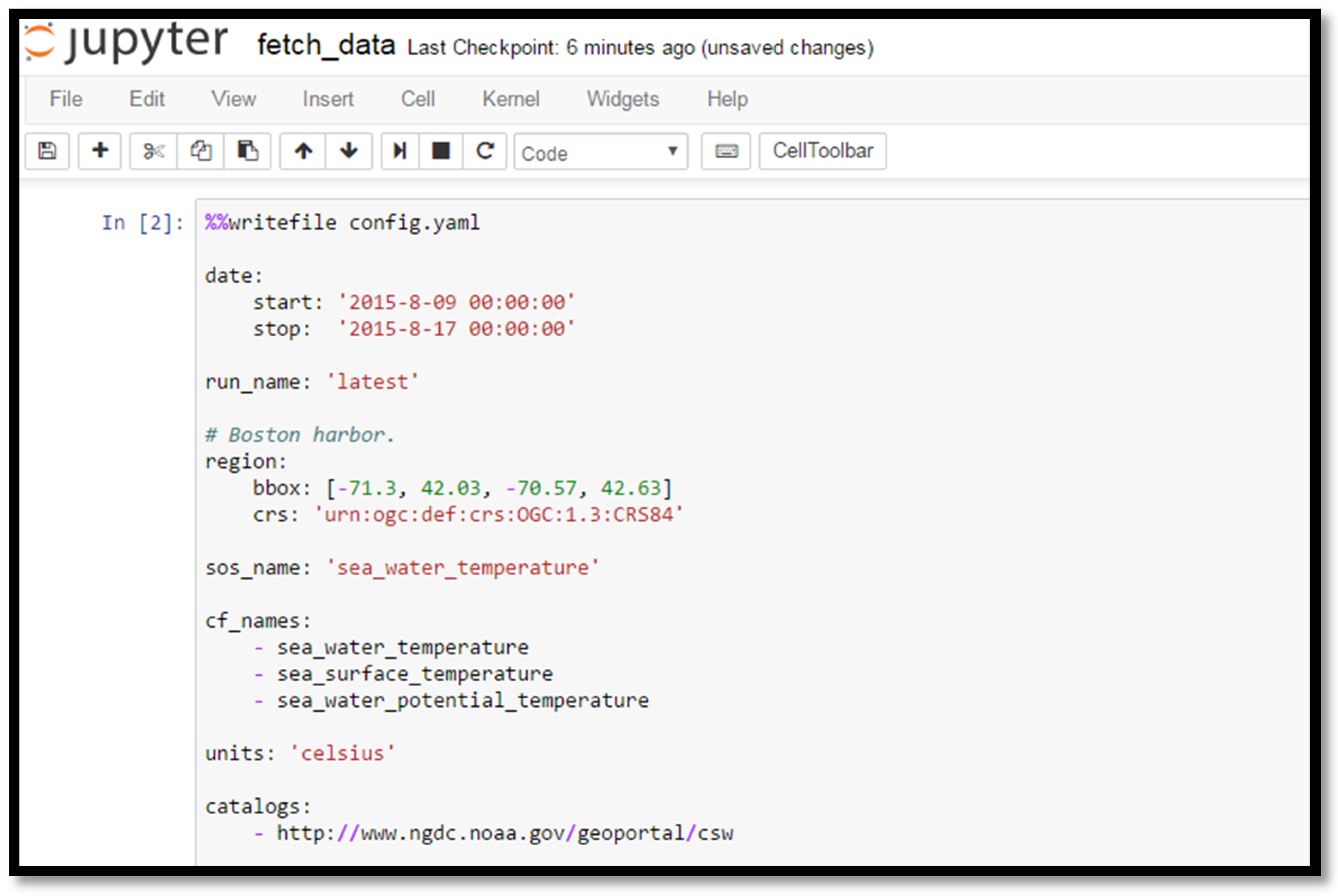
The specific example used in the Boston Light Swim is shown in Figure 4.

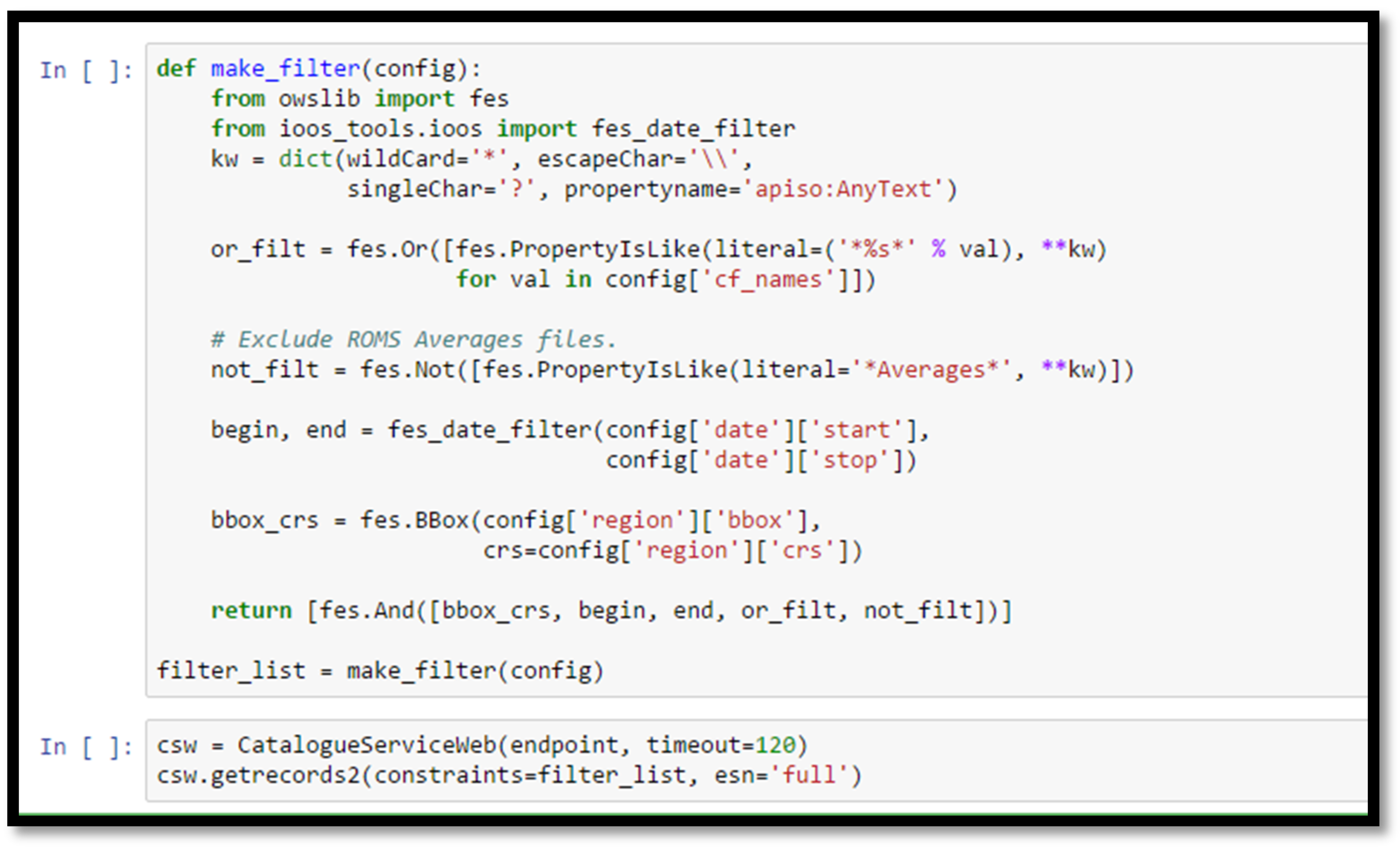
The notebook uses this information and the OWSLib package [26] to construct the CSW query and parse the CSW responses. The CSW query used here is quite sophisticated: we search records that contain any of our list of CF standard names, eliminate records that contain the string Averages, and then select only those records that contain data within the bounding box and time extent window (Figure 5).

From these records we then search for OPeNDAP and SOS service URLs, since our workflow knows how to extract data from these two data service endpoints. Then using the IOOS-developed pyoos package [27], observed data are extracted from the SOS data URLs using high level routines from both NOAA NDBC and NOAA CO-OPS SOS services. The data are then interpolated onto a common hourly time base to facilitate comparison.

With the observed data extracted, we loop through the OPeNDAP URLs, opening the URLs using the British Met Office-developed iris package [28], which uses the CF conventions to allow model-independent extraction of simulation data together with corresponding temporal and geospatial coordinate information. This allows model-independent extraction of simulated time series at the grid cell closest to the observed data. The extracted model time series is then interpolated onto the same one-hour time base to facilitate model-data comparison. The observed and modeled time series data are then saved to disk, ready to be loaded into the Skill Score notebook.

2.4. Skill Score Notebook

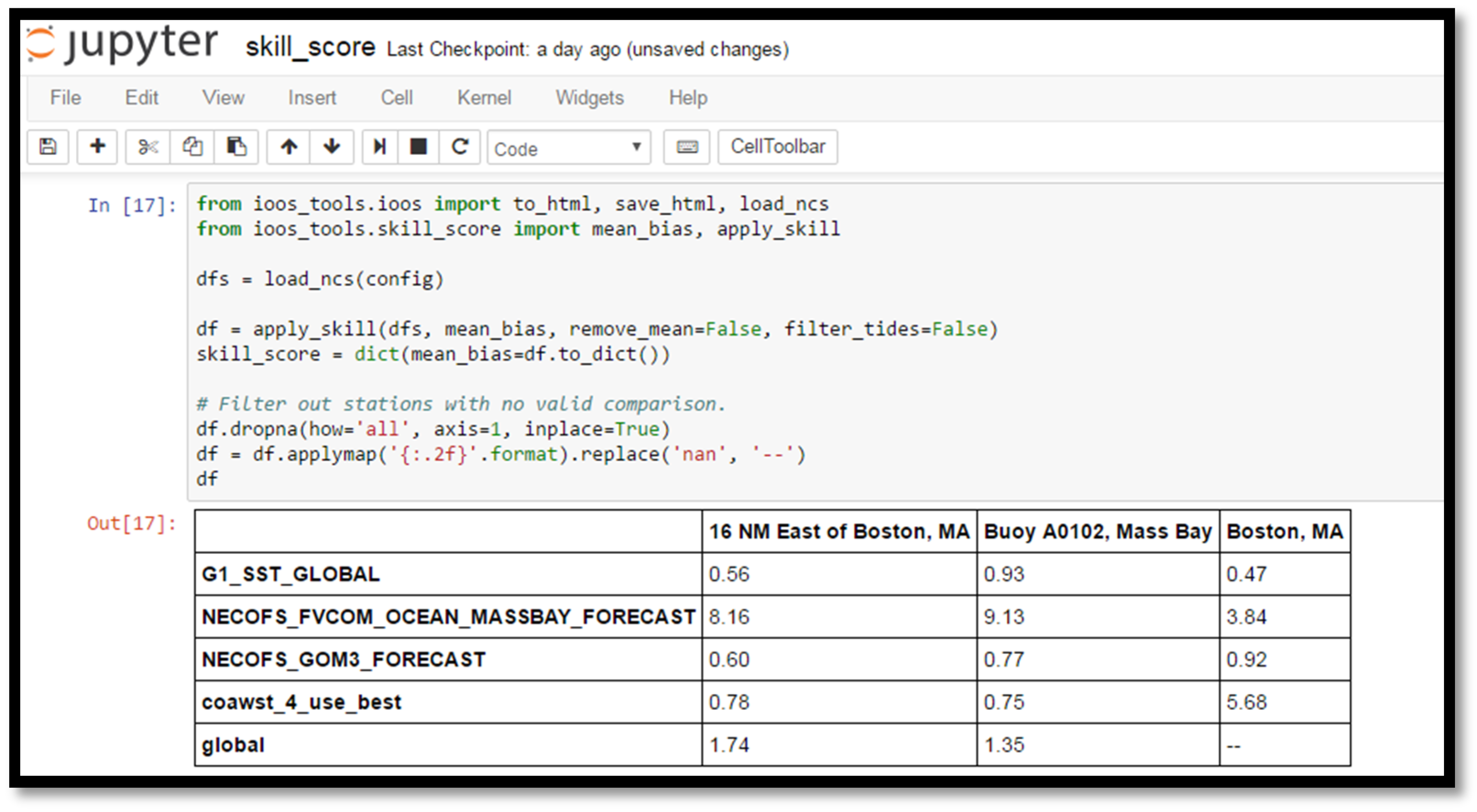
This notebook loads the time series data from observations and models from the Fetch Data notebook and computes a variety of skill metrics, including model bias, central root mean squared error, and correlation (Figure 6). It makes use of the scikit-learn package [29] for skill metrics, and the pandas [30] package for reading and manipulating time series and data frames. The skill metrics are stored on disk for use in the Map Display notebook.

2.5. Map Display Notebook

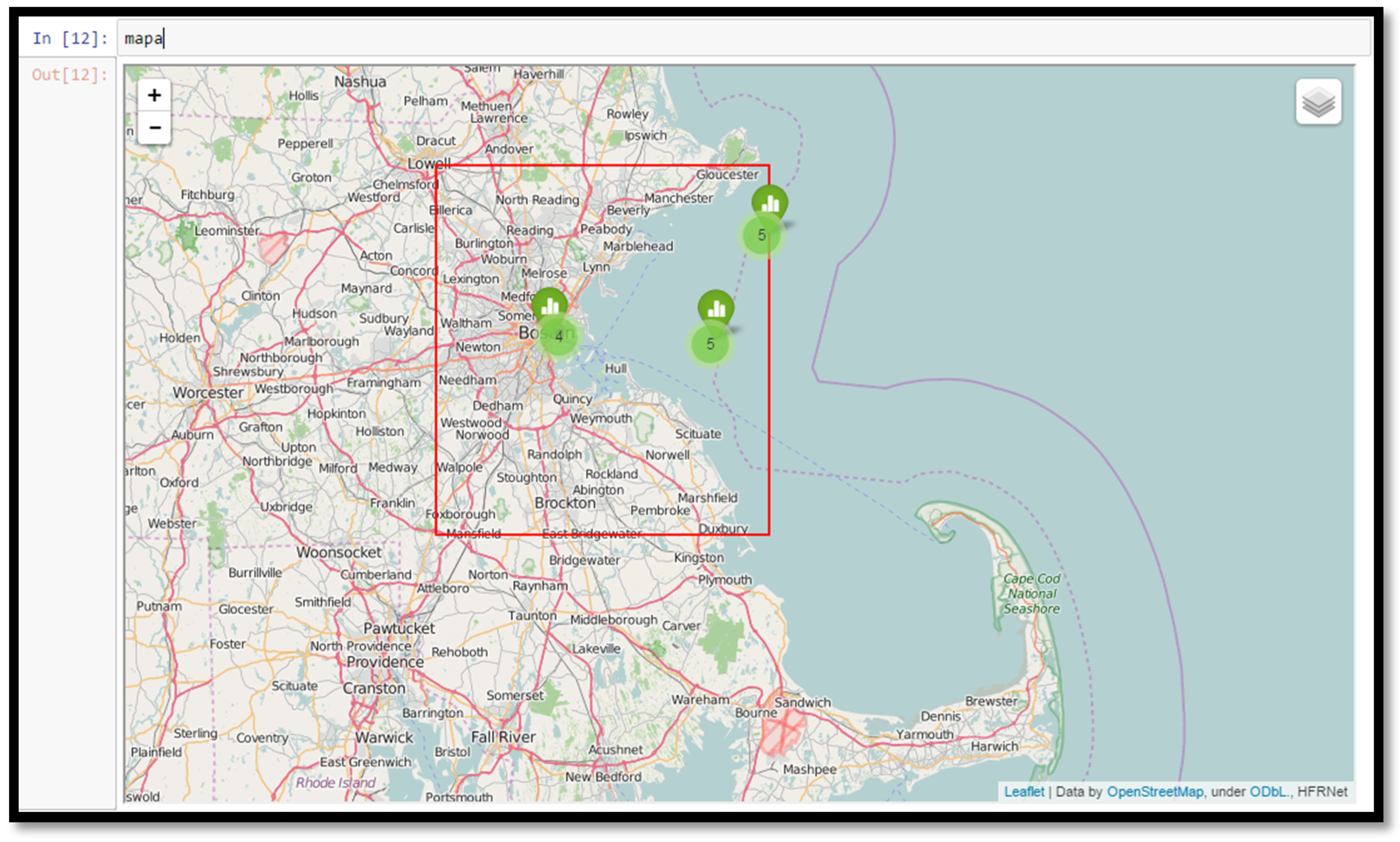
This notebook loads the previously-saved time series data and skill metrics and displays them on an interactive map (Figure 7). The bokeh package [31] is used to automatically create JavaScript plots that are embedded in the notebook, allowing the user to see data locations on a map and click on them to see interactive plots of the time series comparison, along with certain skill metrics. The user can also see the locations of the nearest model grid cells where the time series were extracted to compare with data.

3. Results

The workflow executed with the 2015 Boston Light Swim input parameters discovered in situ temperature data from NOAA NDBC buoys and University of Maine buoys offshore in Massachusetts Bay, and from NOAA CO-OPS tide stations inshore in Boston Harbor (Figure 7). The workflow also discovered temperature data from a remotely-sensed dataset and from four different forecast models that cover the region.

The remotely-sensed data was a daily global product derived from multiple sensors and gap-filled via interpolation over cloudy regions (G1_SST_GLOBAL), while the forecast products discovered were:

• The HYCOM global model run by NCEP, a regular grid model with 9.25 km resolution that assimilates temperature data (HYCOM);
• The COAWST East and Gulf Coast model run by the U.S. Geological Survey, a regular grid model with 5 km resolution that does not directly assimilate data, but indirectly assimilates data by nudging the temperature field toward the HYCOM model (COAWST);
• The NECOFS Gulf of Maine model run by UMASS Dartmouth, a triangular mesh model with variable resolution from 1500 m offshore in Massachusetts Bay to 500 m in Boston Harbor, that assimilates temperature data (NECOFS-GOM)
• The NECOFS Massachusetts Bay model run by UMASS Dartmouth, a triangular mesh model with variable resolution from 1500 m offshore in Massachusetts Bay to 100 m in Boston Harbor, that does not assimilate temperature data (NECOFS-MassBay)

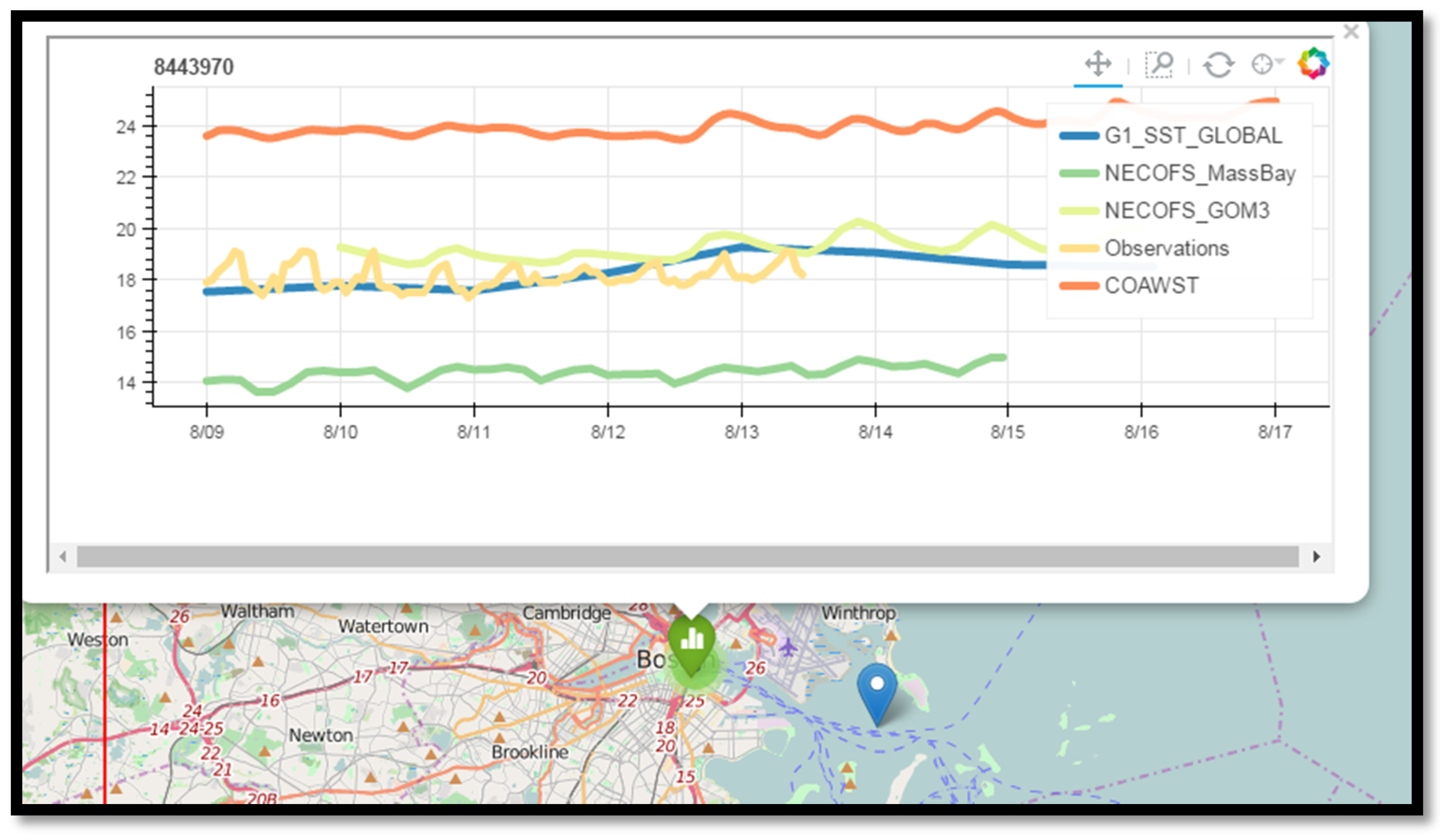
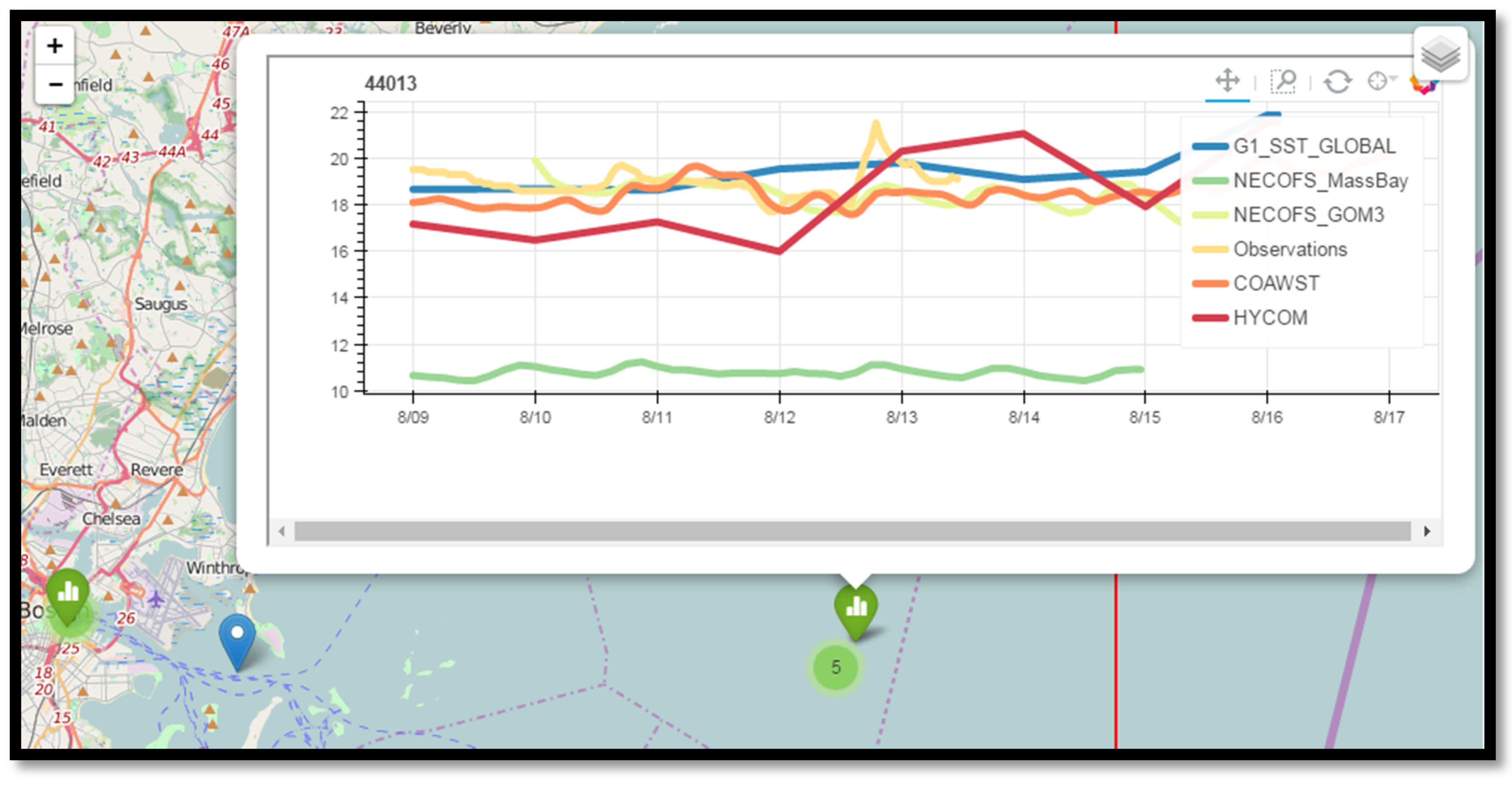
The results showed that two models had significant biases with respect to the data. The COAWST model was too warm in Boston Harbor by about 6 °C (Figure 8), and the highest resolution NECOFS-MassBay model was too cold at all three locations—nearly 8 °C off at the Boston Buoy (Figure 9) and at the NERACOOS Buoy A (not shown, as similar to the Boston Buoy). The lowest resolution HYCOM model and the NECOFS-GOM model were relatively close at all three locations, with average biases less than 2 °C.

To further investigate the issues with the COAWST and NECOFS-MassBay models, we extracted the simulated temperature fields over the entire domain from both models.

The COAWST temperature field showed multiple hot spots along the coast, including Boston Harbor (not shown). Further investigation with the COAWST forecast modelers revealed that these hot spots were regions outside the domain of the HYCOM model from which temperatures were being nudged. Within these regions, temperatures were getting assigned to 25 °C, instead of using the nearest HYCOM values. This issue was promptly corrected by the modelers.

The NECOFS-MassBay temperature field showed uniformly cold temperatures throughout the domain, with the exception of a thin band of water along the open boundary (not shown). Further investigation with the NECOFS-MassBay modelers revealed that the NECOFS-MassBay model temperature field is forced by the NECOFS-GOM model along the open boundary, and that the atmospheric model used to drive both the NECOFS-GOM and NECOFS-MassBay model has too many clouds, and therefore underrepresents, the amount of short-wave radiation into the ocean. In the NECOFS-GOM model, this problem is masked because the model assimilates remotely-sensed SST data, but in the NECOFS-MassBay model, the modelers assumed the domain was small enough that the NECOFS-GOM forcing along the boundary would be sufficient to control the temperature field and, therefore, no temperature data was assimilated. The findings here showed this assumption needs reevaluation.

With confidence that the bias in the NECOFS-MassBay model was consistent over the region of the Boston Light Swim, we provided the swimmers with bias-corrected forecast maps from the NECOFS-MassBay model for each hour of the race. The swimmers reported that these corrected maps were very useful and were within 1–2 °C of temperatures observed during the swim.

4. Discussion

The use of dynamic, reusable workflows has a number of technological and scientific benefits. The use of the catalog allows data to be discovered dynamically, and the reproducible workflow means the results can be verified by others and used to create entirely new workflows. In fact, the set of sea surface temperature skill-assessment notebooks used here was derived from a set of water level skill-assessment notebooks developed for the IOOS System Test [13]. We simply changed the CF Standard Names from specifying sea surface height to specifying sea water temperature.

The fact that the notebook is driven by a catalog search means that it dynamically discovers new data that are available (and drops data that are no longer available!). When one of the authors (R.S.) was testing the notebook before a presentation, he was surprised (and delighted) to find a new model appearing in the skill assessment plot because another modeling group had registered their data with the catalog service. It is also not necessary to limit the search to one catalog service endpoint. Although we only used the IOOS CSW service for this 2015 Boston Light Swim example, a list of endpoints can be used, and we now include the data.gov CSW service as well.

To reproduce the workflow, the notebook must be shared, but also the environment necessary to run the notebook must be shared. This has traditionally been challenging, as sets of notebooks, like the one discussed here, depend on many packages, some with binary dependencies that can be tricky to build on all major platforms. Luckily, with the rise of technologies like GitHub [32], docker [33], Anaconda Python [34], conda [35], and conda-forge [36], services like binder [37] can now allow users to view a rendered notebook on GitHub, complete with embedded code, output, and graphics, and then click a button that starts up a notebook server on the Cloud, provisioned with the appropriate environment to run that notebook. Users can just click “run all” to execute the workflow, without installing anything locally, and without leaving their web browser.

Making it easy to conduct automated skill assessments has a number of other benefits as well. For modelers, it means they can spend more time on science, and less time performing mundane data tasks. For users, it means they can conduct their own skill assessment of existing models, instead of relying only on the modelers themselves. This is particularly important now that there are realistic regional and global simulations that are far beyond the ability of the modelers to test for all possible uses.

The success of this dynamic, reusable workflow shows what can happen when a community agrees on a common set of web services and a common vocabulary. In this case the participants did not already have an established vocabulary or established custom services, so IOOS provided best-practice suggestions for both software and service configuration to enable their approved services. IOOS data providers who wish to have their data plugged into the system can either follow the procedures described in [22] or see if one of the regional associations or Federal backbone partners can host their data and provide services. To enable workflows like this across communities with a variety of established services and vocabularies, brokering approaches for web services [38] and semantic approaches [39] will be necessary.

This workflow demonstrates the power of the dynamic, reusable workflow approach, but there are caveats and room for future improvements:

• Notebooks allow rich documentation, but it is still up to the developer to describe the workflow, use clear variable names and produce well-structured, readable code.
• While the software in dynamic workflows is always reproducible, the results of a specific workflow may not be reproducible if the data sources no longer exist or have changed.
• Workflow developers cannot expect standardized services and metadata to solve all data-wrangling problems. Some time and expertise is typically still needed to adapt discovered data sources to a specific workflow.
• Tools for standardized catalog and data service access need to be developed beyond Python, to support other major scientific analysis languages and environments used by scientists and developers (e.g., MATLAB, R, JavaScript, Julia, ArcGIS).
• Better documentation and support is needed to document how users can take advantage of workflows like this, and also for providers to connect their data to standardized services
• As data and catalog services become more heavily used, the software supporting these services needs to be made more robust and scalable. Requests to the THREDDS Data Server, for example, are single-threaded, and many simultaneous requests can overwhelm the server.
• The examples in this paper used nearest-neighbor lookup to extract time series from models. For more sophisticated interpolation schemes, tools that work with the topology of unstructured and staggered grid model output are required, taking advantage of the UGRID [40] and SGRID [41] conventions the community has developed.
• While it is possible to run the notebooks without understanding the details of the coding, it currently does require understanding of how to run a notebook (e.g., launch the binder service, navigate to the notebook, click on “run all” under the “cell” drop-down menu). Tools for deploying notebooks as simple web apps that hide this complexity from users are in development by the Jupyter team.

5. Conclusions

There are a number of benefits to developing dynamic, reusable workflows. Through catalog searches and use of interoperable web services they enable more effective assessment of large, distributed collections of data, such as numerical model results. More eyes on the model results means more feedback to modelers, resulting in better models. Complex data analysis from a variety of sources can be automated and dynamically respond as new data enter (or leave) the system. The notebook approach allows rich documentation of the workflow, and automatic generation of software environments allow users to easily run specific notebooks on local computers, on remote machines, or in the Cloud. The workflows also serve as training by example for potential users of standardized catalogs and data services, as well as demonstrating the type of custom workflow elements typically required for success. The workflows can also be easily modified to form the basis for new scientific applications. Often a new application will highlight issues that need fixing before it can function. Sometimes these are minor metadata or service issues that can easily be fixed by providers, and sometimes these are more major issues that require further research and development of standards, services, or tools. Regardless of the issue, fixing it for a specific workflow not only enables success for that workflow, but for an entire class of workflows and, thus, the larger geoscience community. With their numerous benefits demonstrated here, we anticipate dynamic, reusable workflows will become more common and expanded to more applications, services, and geoscience domains.

To reproduce the Boston Light Swim notebooks, visit IOOS Notebooks Demos on GitHub [42] and follow the instructions to install and run locally, or click the run “launch binder” button to run remotely on the Cloud.

References

- Global Change Master Directory. Available online: http://gcmd.nasa.gov (accessed on 2 September 2016).
- GEOSS Portal. Available online: http://www.geoportal.org (accessed on 2 September 2016).
- Zdenka, W.; Manley, J. Ocean Observing: Delivering the Benefits. Mar. Technol. Soc. J. 2010, 44, 4–5. [Google Scholar] [CrossRef]
- Robert, B.; Beard, R.; Burnett, W.; Crout, R.; Griffith, B.; Jensen, R.; Signell, R. Implementing the National Integrated Ocean Observing System (IOOS®)—From the Federal Agency Perspective. Mar. Technol. Soc. J. 2010, 44, 32–41. [Google Scholar] [CrossRef]
- OGC Sensor Observation Service. Available online: http://www.opengeospatial.org/standards/sos (accessed on 7 September 2016).
- ERDDAP. Available online: http://coastwatch.pfel.noaa.gov/erddap/index.html (accessed on 7 September 2016).
- OPeNDAP. Available online: https://www.opendap.org (accessed on 7 September 2016).
- Climate and Forecast Metadata Conventions. Available online: http://cfconventions.org (accessed on 7 September 2016).
- ISO 19115-2 Metadata. Available online: http://www.iso.org/iso/home/store/catalogue_tc/catalogue_detail.htm?csnumber=67039 (accessed on 7 September 2016).
- De La Beaujardière, J.; Beegle-Krause, C.J.; Bermudez, L.; Hankin, S.; Hazard, L.; Howlett, E.; Le, S.; Proctor, R.; Signell, R.P.; Snowden, D.; et al. Ocean and Coastal Data Management. Eur. Space Agency 2010, 226–236. [Google Scholar] [CrossRef]
- Hankin, S.; Bermudez, L.; Blower, J.D.; Blumenthal, B.; Casey, K.S.; Fornwall, M.; Graybeal, J.; Guralnick, R.P.; Habermann, T.; Howlett, E.; et al. NetCDF-CF-OPeNDAP: Standards for Ocean Data Interoperability and Object Lessons for Community Data Standards Processes. Eur. Space Agency 2010, 450–458. [Google Scholar] [CrossRef]
- Helen, S. Interactive Notebooks: Sharing the Code. Nature 2014, 515, 151–152. [Google Scholar]
- IOOS System Test Wiki. Available online: https://github.com/ioos/system-test/wiki (accessed on 2 September 2016).
- Jupyter Project. Available online: http://jupyter.org (accessed on 7 September 2016).
- THREDDS Data Server. Available online: http://www.unidata.ucar.edu/software/thredds/current/tds/ (accessed on 7 September 2016).
- Network Common Data Form. Available online: http://www.unidata.ucar.edu/software/netcdf/ (accessed on 7 September 2016).
- NetCDF Markup Language. Available online: http://www.unidata.ucar.edu/software/thredds/current/netcdf-java/ncml/ (accessed on 7 September 2016).
- Signell, R.P.; Carniel, S.; Chiggiato, J.; Janekovic, I.; Pullen, J.; Sherwood, C.R. Collaboration Tools and Techniques for Large Model Datasets. J. Mar. Syst. 2008, 69, 154–161. [Google Scholar] [CrossRef]
- Signell, R.P. Model Data Interoperability for the United States Integrated Ocean Observing System (IOOS). Am. Soc. Civ. Eng. 2010, 221–238. [Google Scholar] [CrossRef]
- Bergamasco, A.; Benetazzo, A.; Carniel, S.; Falcieri, F.M.; Minuzzo, T.; Signell, R.P.; Sclavo, M. Knowledge Discovery in Large Model Datasets in the Marine Environment: The THREDDS Data Server Example. Adv. Oceanogr. Limnol. 2012, 3, 41–50. [Google Scholar] [CrossRef]
- Signell, R.P.; Snowden, D.P. Advances in a Distributed Approach for Ocean Model Data Interoperability. J. Mar. Sci. Eng. 2014, 2, 194–208. [Google Scholar] [CrossRef]
- Signell, R.P.; Camossi, E. Technical Note: Harmonising Metocean Model Data via Standard Web Services within Small Research Groups. Ocean Sci. 2016, 12, 633–645. [Google Scholar] [CrossRef]
- ncISO. Available online: http://www.ngdc.noaa.gov/eds/tds/ (accessed on 7 September 2016).
- CKAN. Available online: http://ckan.org (accessed on 7 September 2016).
- pycsw. Available online: http://pycsw.org (accessed on 7 September 2016).
- OWSLib. Available online: https://geopython.github.io/OWSLib (accessed on 7 September 2016).
- pyoos. Available online: https://github.com/ioos/pyoos (accessed on 7 September 2016).
- iris. Available online: http://scitools.org.uk/iris/ (accessed on 7 September 2016).
- pandas. Available online: http://pandas.pydata.org (accessed on 7 September 2016).
- scikit-learn. Available online: http://scikit-learn.org (accessed on 8 September 2016).
- bokeh. Available online: http://bokeh.pydata.org (accessed on 7 September 2016).
- GitHub. Available online: http://github.com (accessed on 7 September 2016).
- Docker. Available online: http://www.docker.com (accessed on 7 September 2016).
- Anaconda Python. Available online: https://docs.continuum.io/anaconda/ (accessed on 7 September 2016).
- conda. Available online: http://conda.pydata.org/docs/index.html (accessed on 7 September 2016).
- conda-forge. Available online: https://conda-forge.github.io (accessed on 7 September 2016).
- Binder. Available online: http://mybinder.org/ (accessed on 7 September 2016).
- Nativi, S.; Craglia, M.; Pearlman, J. Earth Science Infrastructures Interoperability: The Brokering Approach. IEEE J. Sel. Top. Appl. Earth Obs. Remote Sens. 2013, 6, 1118–1129. [Google Scholar] [CrossRef]
- Fox, P.; McGuinness, D.; Middleton, D.; Cinquini, L.; Darnell, J.A.; Garcia, J.; West, P.; Benedict, J.; Solomon, S. Semantically-Enabled Large-Scale Science Data Repositories. In The Semantic Web—ISWC 2006; Cruz, I., Decker, S., Allemang, D., Preist, C., Schwabe, D., Mika, P., Uschold, M., Aroyo, L.M., Eds.; Springer: Heidelberg/Berlin, Germany, 2006; Volume 4273, pp. 792–805. Available online: http://link.springer.com/10.1007/11926078_57 (accessed on 7 September 2016).
- UGRID Conventions. Available online: http://ugrid-conventions.github.io/ugrid-conventions (accessed on 2 September 2016).
- SGRID Conventions. Available online: http://sgrid.github.io/sgrid (accessed on 2 September 2016).
- IOOS Notebook Demos. Available online: https://github.com/ioos/notebooks_demos (accessed on 2 September 2016).
© 2016 by the authors; licensee MDPI, Basel, Switzerland. This article is an open access article distributed under the terms and conditions of the Creative Commons Attribution license ( http://creativecommons.org/licenses/by/4.0/).