Figure 1.
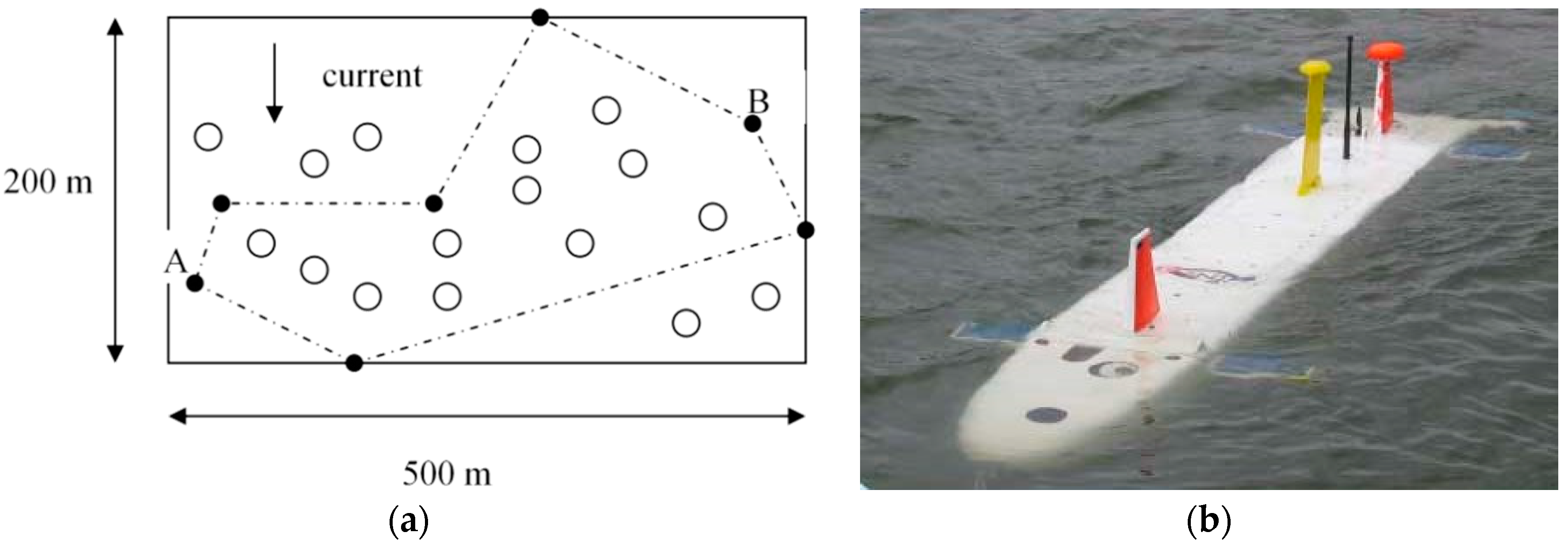
Submersible vehicle sample and notional minefield [
1]. (
a) Field of randomly-placed submersed mines to be avoided by the autonomous vehicle; and (
b)
Aries submersible in open ocean (illustrative sample is not simulated; the
Figure 2 Phoenix vehicle is simulated).
Figure 1.
Submersible vehicle sample and notional minefield [
1]. (
a) Field of randomly-placed submersed mines to be avoided by the autonomous vehicle; and (
b)
Aries submersible in open ocean (illustrative sample is not simulated; the
Figure 2 Phoenix vehicle is simulated).
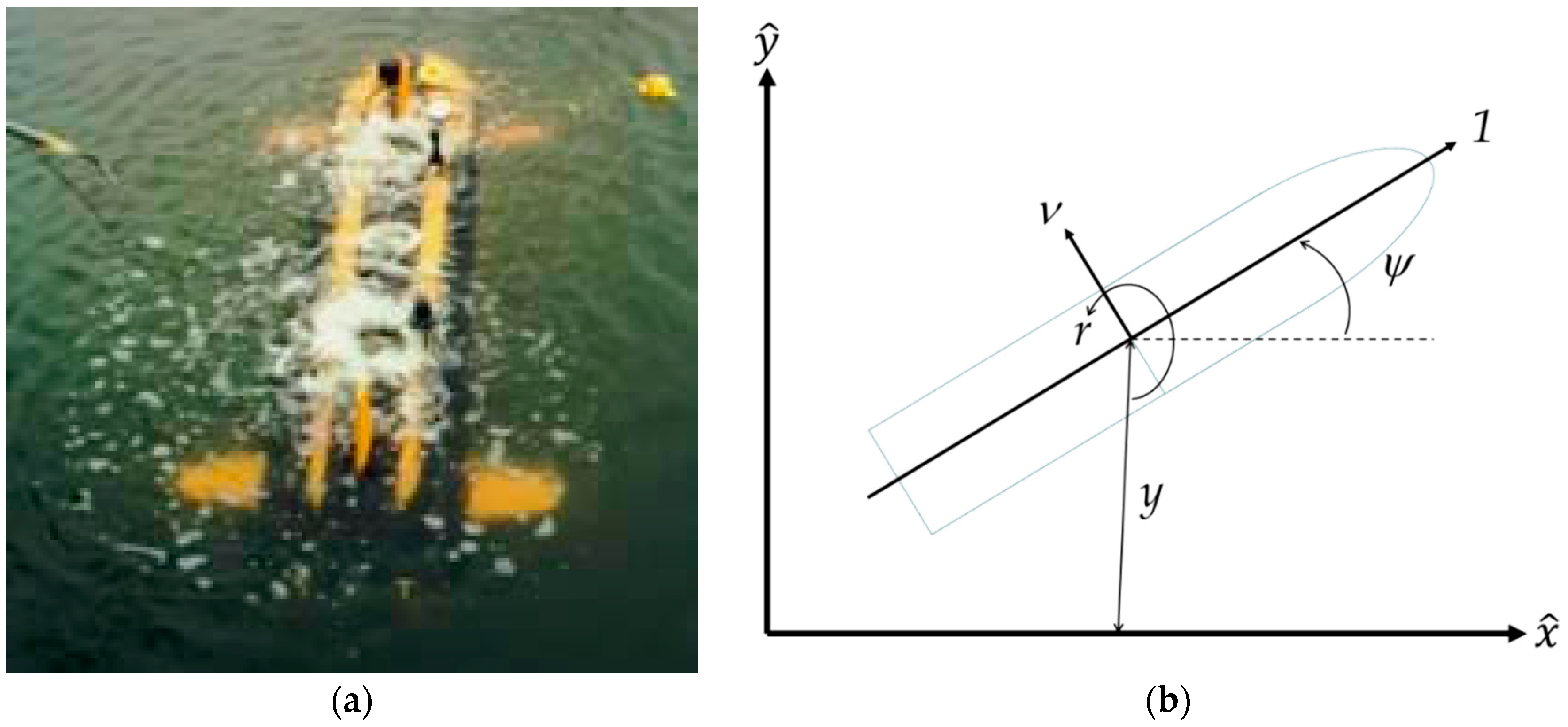
Figure 2.
Vehicle geometry and reference axes. (
a)
Phoenix in open ocean [
1]. The experimentally-determined dynamic model for this vehicle is listed in Equations (1)–(6) and forms the basis for the simulations in this manuscript; and (
b) vehicle geometry and reference axis.
Figure 2.
Vehicle geometry and reference axes. (
a)
Phoenix in open ocean [
1]. The experimentally-determined dynamic model for this vehicle is listed in Equations (1)–(6) and forms the basis for the simulations in this manuscript; and (
b) vehicle geometry and reference axis.
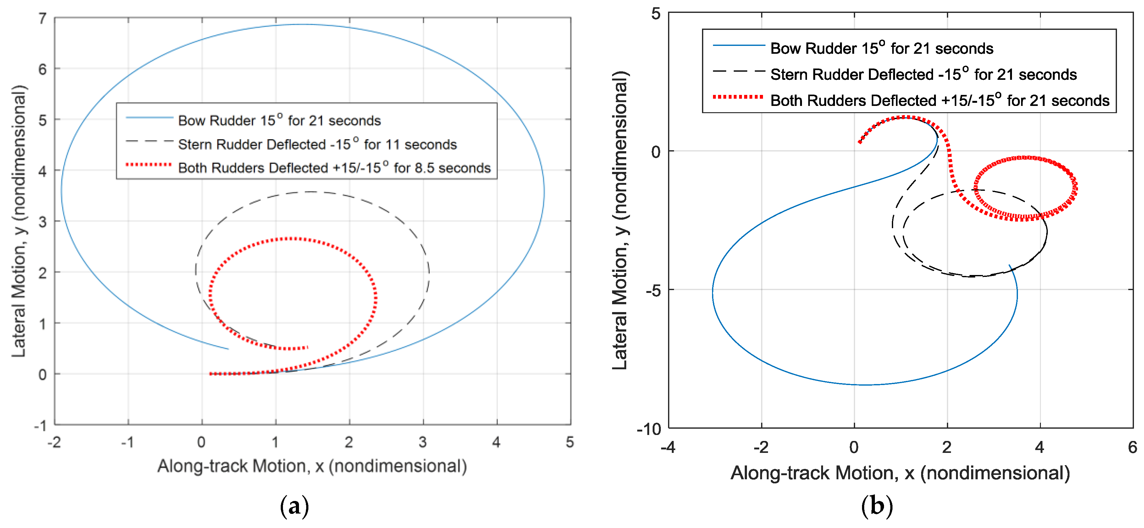
Figure 3.
Analysis of uncontrolled system: comparison of rudder performance. (a) Counter-clockwise turn, ; and (b) initial sway velocity .
Figure 3.
Analysis of uncontrolled system: comparison of rudder performance. (a) Counter-clockwise turn, ; and (b) initial sway velocity .
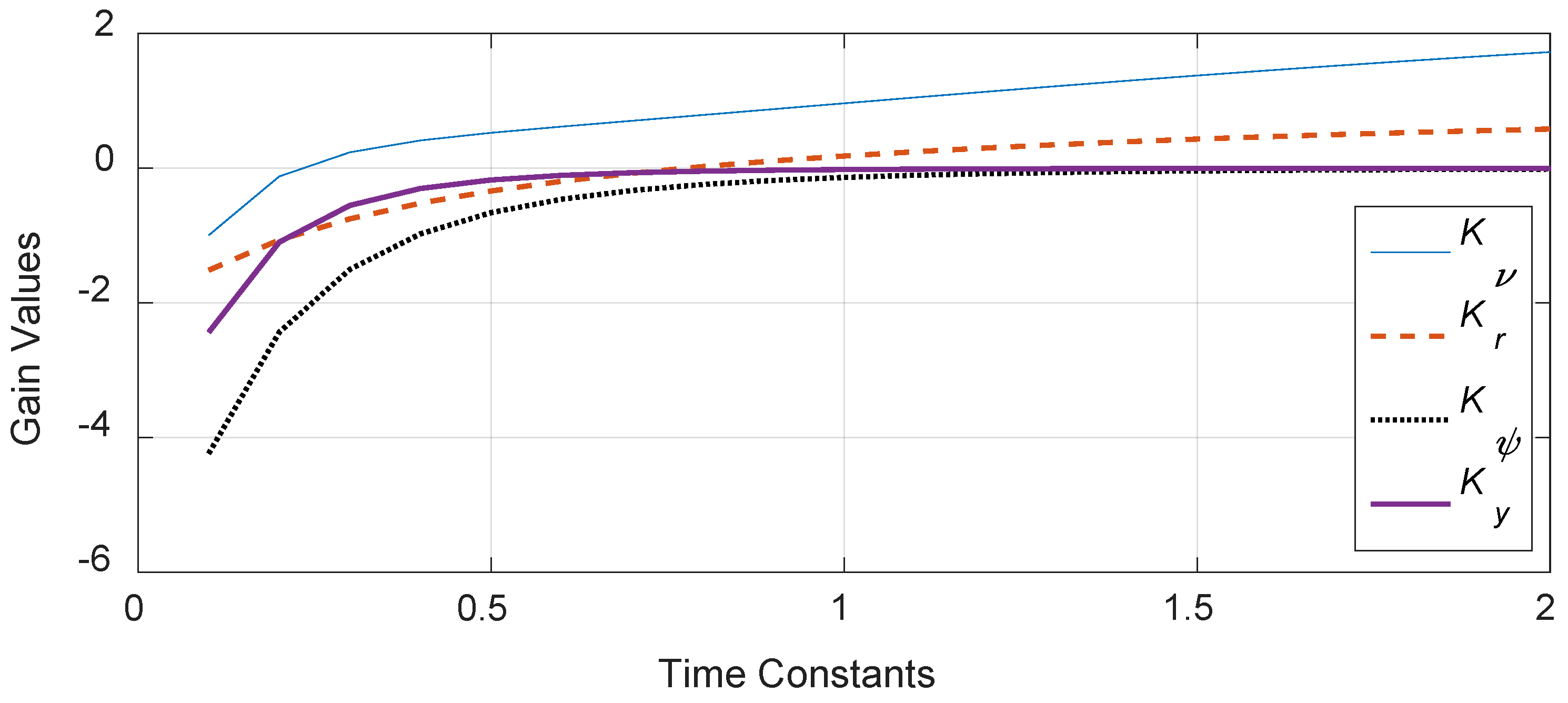
Figure 4.
Gain values for each state iterated for various time constants.
Figure 4.
Gain values for each state iterated for various time constants.
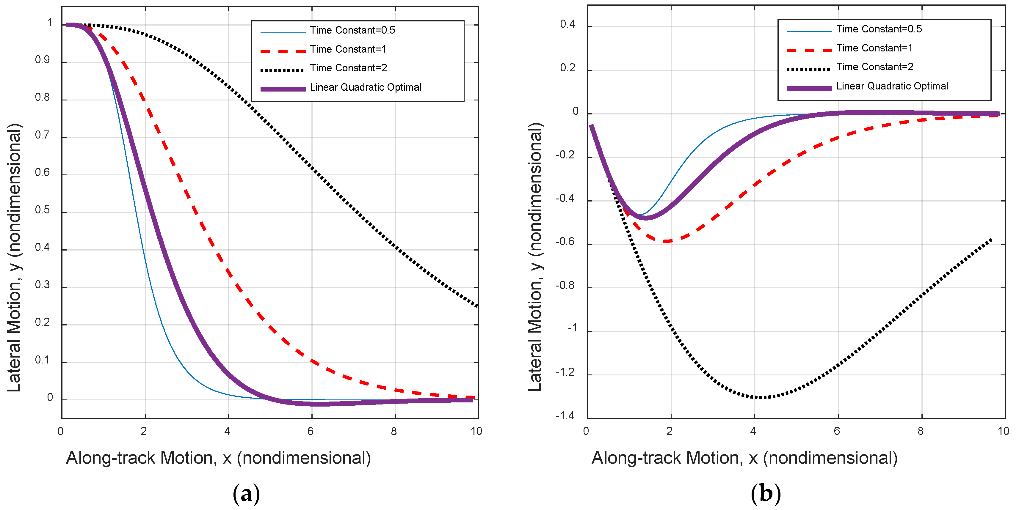
Figure 5.
Simulations testing the initial baseline feedback controller in two scenarios. (a) Initially one ship’s length port side; and (b) initial heading 30° starboard.
Figure 5.
Simulations testing the initial baseline feedback controller in two scenarios. (a) Initially one ship’s length port side; and (b) initial heading 30° starboard.
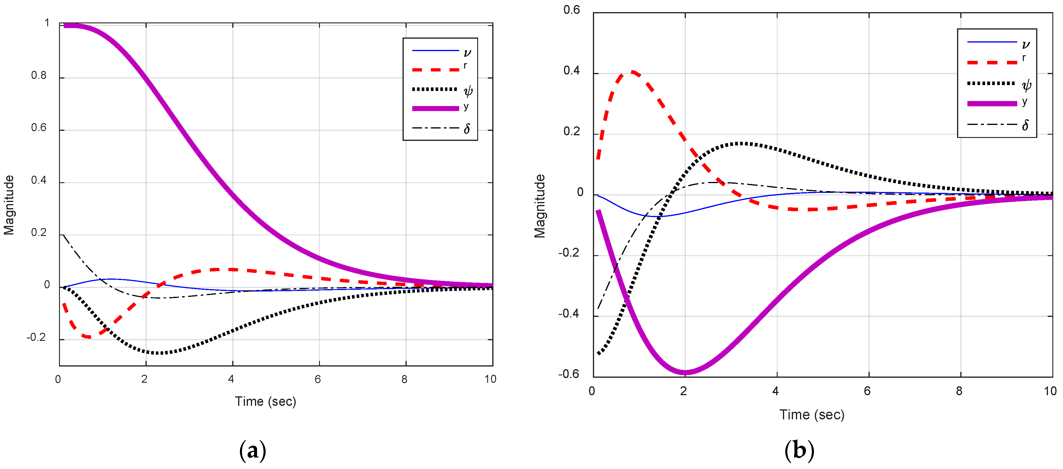
Figure 6.
State variations for both scenarios simulated using pole-placement gains via rule of thumb. (a) Initially one ship’s length port side; and (b) initial heading 30° starboard.
Figure 6.
State variations for both scenarios simulated using pole-placement gains via rule of thumb. (a) Initially one ship’s length port side; and (b) initial heading 30° starboard.
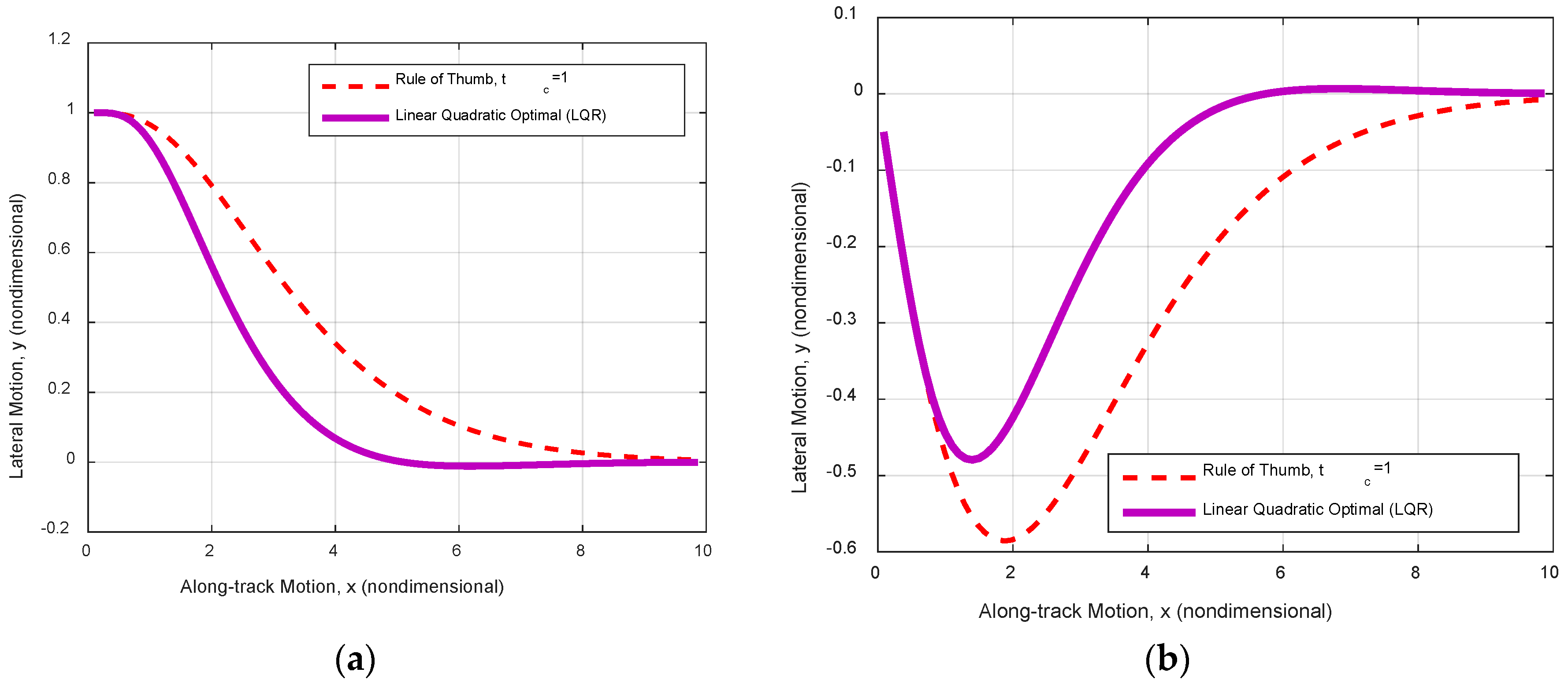
Figure 7.
Rudder-limited trajectory track using pole-placement gains via rule of thumb and LQR. (a) Initially one ship’s length port side; and (b) initial heading 30° starboard.
Figure 7.
Rudder-limited trajectory track using pole-placement gains via rule of thumb and LQR. (a) Initially one ship’s length port side; and (b) initial heading 30° starboard.
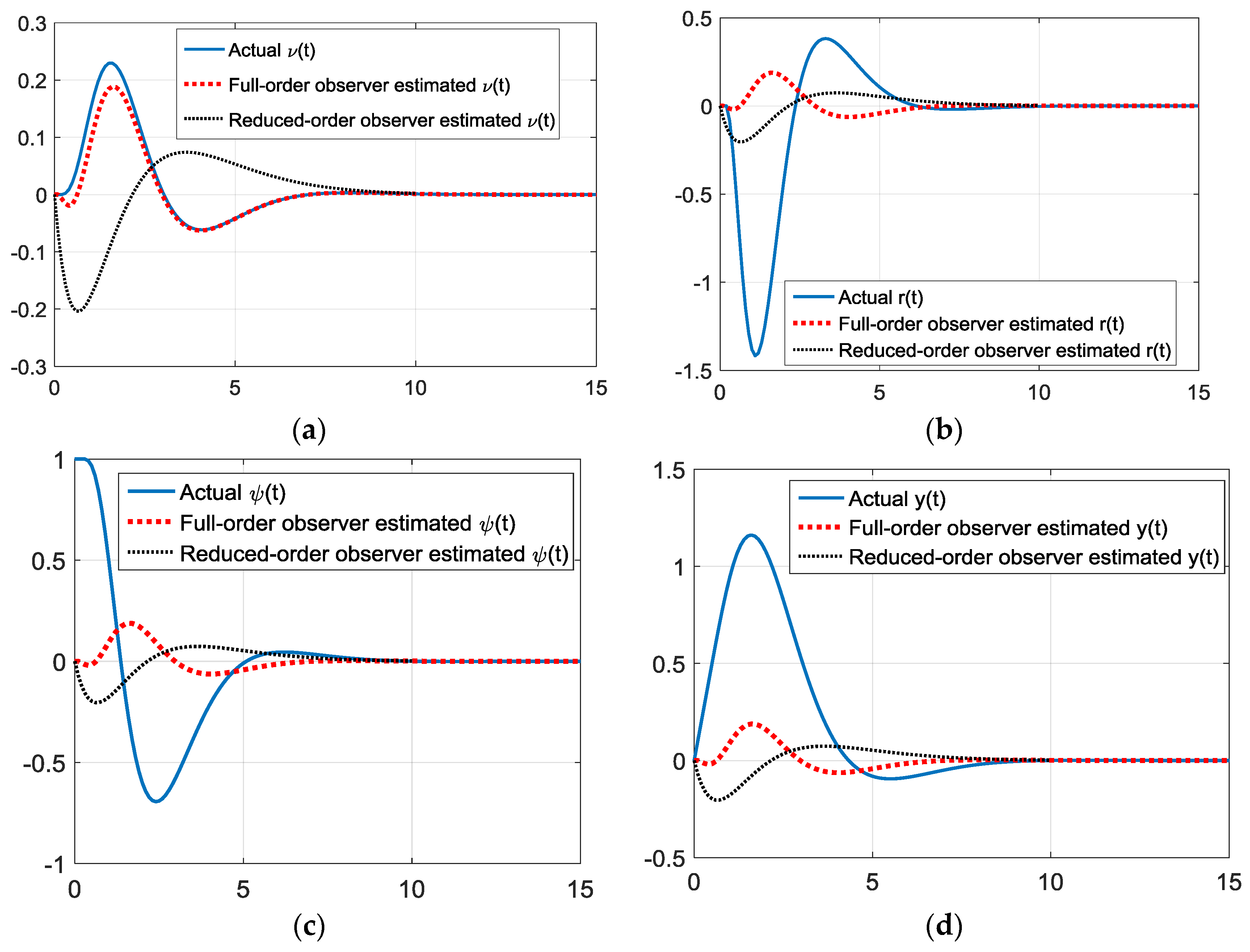
Figure 8.
Simulations starting 30 degrees off heading with gains via rule of thumb state observer gains. (a) True and estimated sway velocity, ν(t); (b) true and estimated turning rate, r(t); (c) true and estimated heading angle, ψ(t); and (d) true and estimated cross track, y(t).
Figure 8.
Simulations starting 30 degrees off heading with gains via rule of thumb state observer gains. (a) True and estimated sway velocity, ν(t); (b) true and estimated turning rate, r(t); (c) true and estimated heading angle, ψ(t); and (d) true and estimated cross track, y(t).
Figure 9.
Simulations starting one boat-length starboard with gains via rule of thumb. (a) True and estimated sway velocity, ν(t); (b) true and estimated turning rate, r(t); (c) true and estimated heading angle, ψ(t); and (d) true and estimated cross track, y(t).
Figure 9.
Simulations starting one boat-length starboard with gains via rule of thumb. (a) True and estimated sway velocity, ν(t); (b) true and estimated turning rate, r(t); (c) true and estimated heading angle, ψ(t); and (d) true and estimated cross track, y(t).
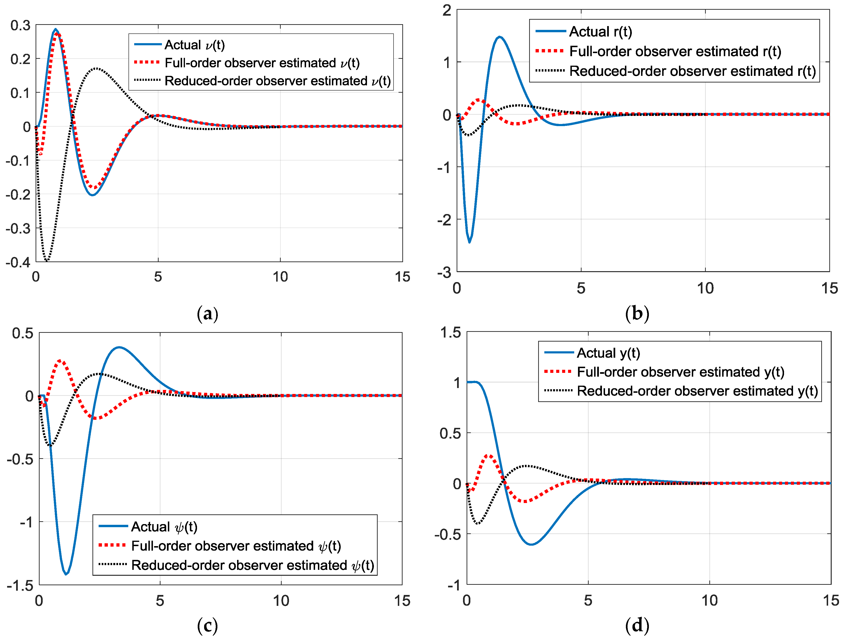
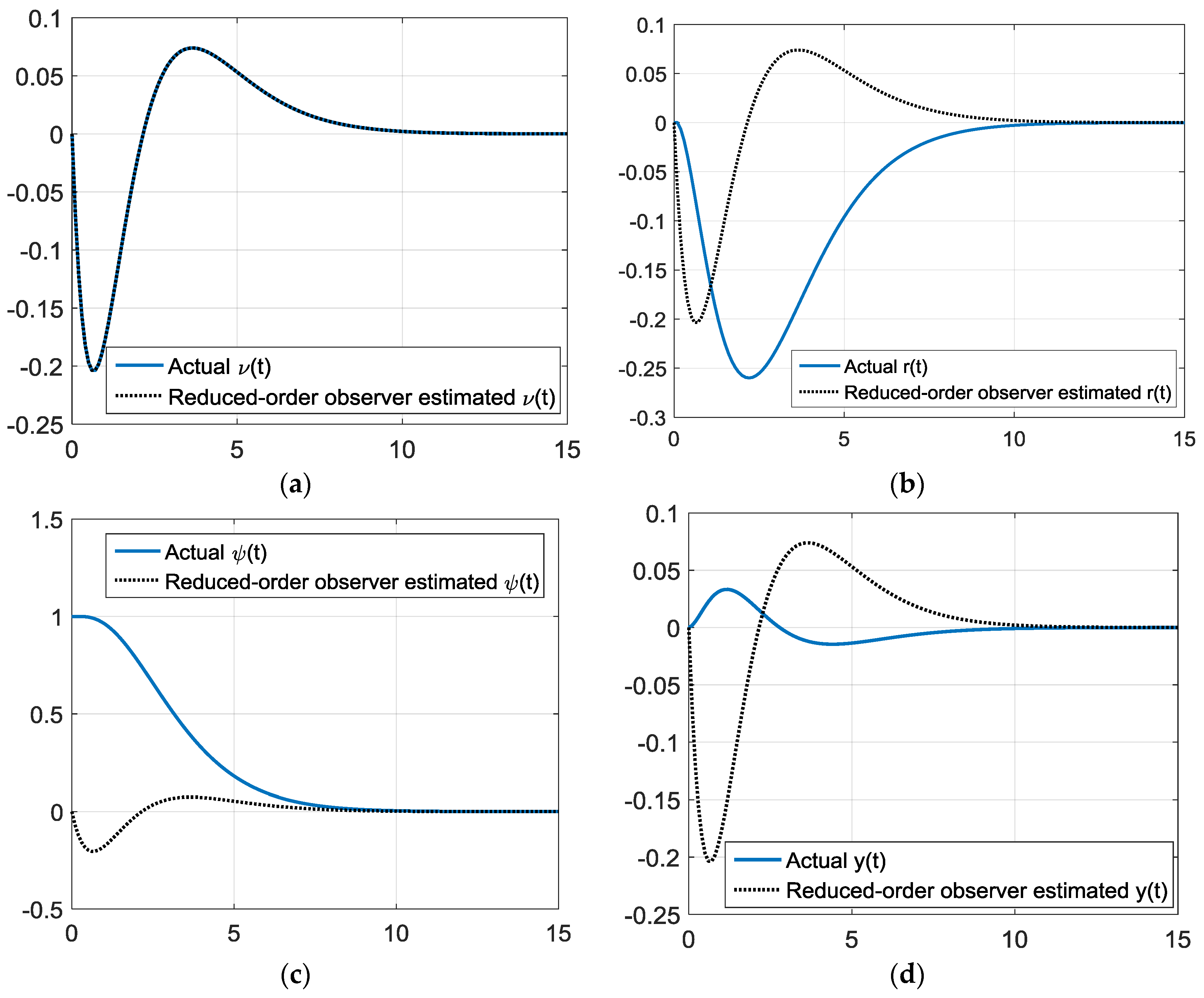
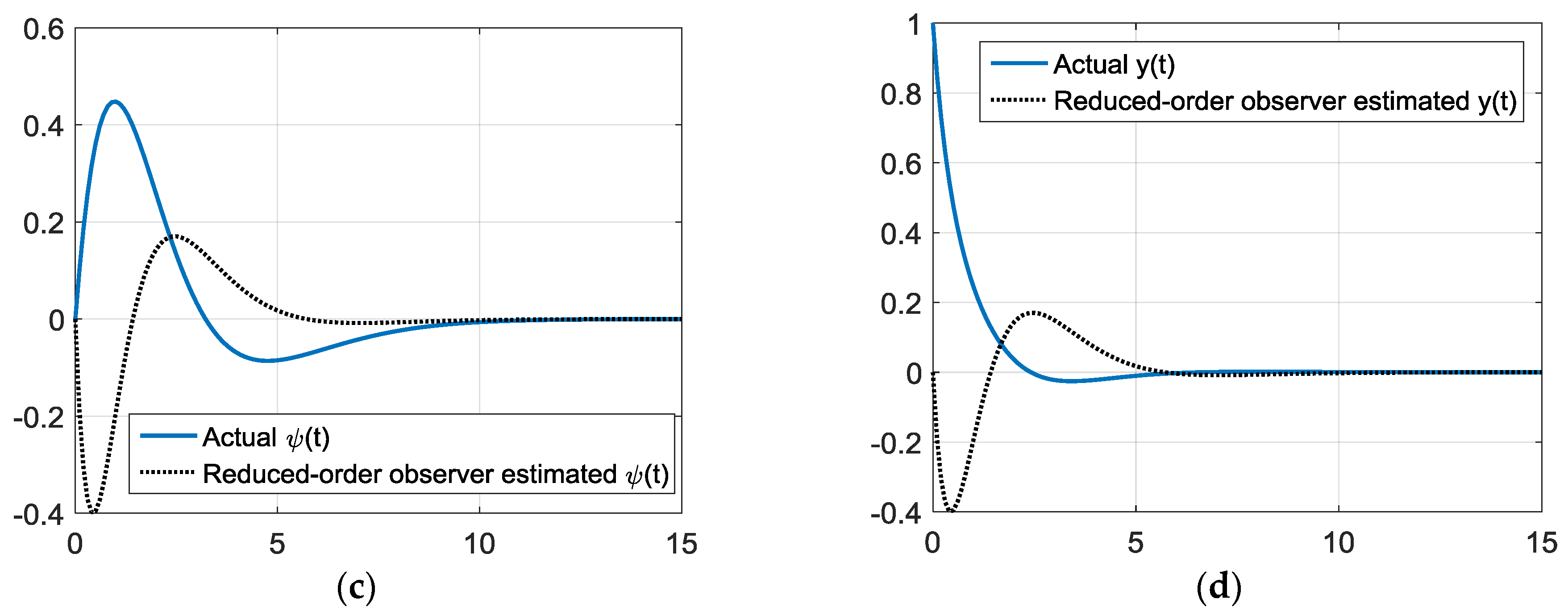
Figure 10.
Simulations starting 30 degrees off heading gains via rule of thumb reduced-order state observer gains. (a) True and estimated sway velocity, ν(t) versus time (seconds); (b) true and estimated turning rate, r(t) versus time (seconds); (c) true and estimated heading angle, ψ(t) versus time (seconds); and (d) true and estimated cross track, y(t) versus time (seconds).
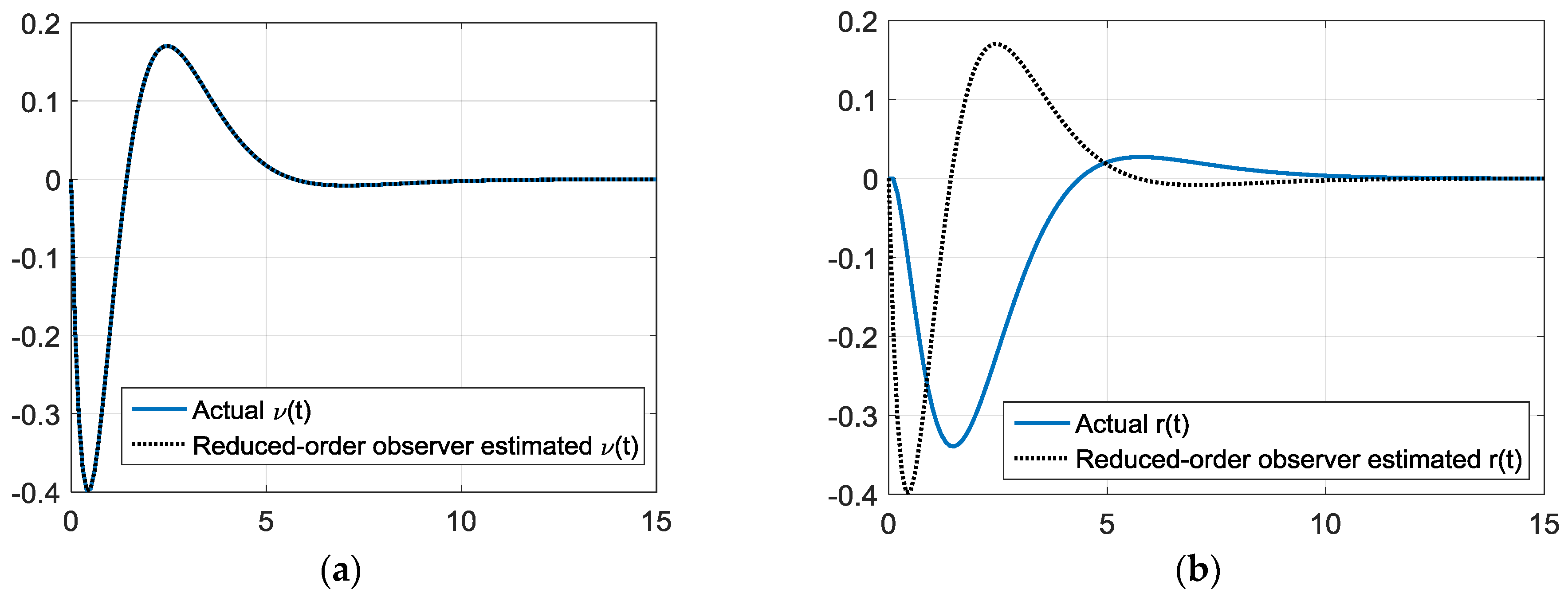
Figure 11.
Simulations starting one boat-length starboard with gains via rule of thumb reduced-order state observer gains. (a) True and estimated sway velocity, ν(t) versus time (seconds); (b) true and estimated turning rate, r(t) versus time (seconds); (c) true and estimated heading angle, ψ(t) versus time (seconds); and (d) true and estimated cross track, y(t) versus time (seconds).
Figure 12.
Infinite gain margin and 80.2° phase margin using full state feedback via full-ordered observer with rule of thumb controller gains. (a) Root locus; and (b) Bode plot.
Figure 12.
Infinite gain margin and 80.2° phase margin using full state feedback via full-ordered observer with rule of thumb controller gains. (a) Root locus; and (b) Bode plot.
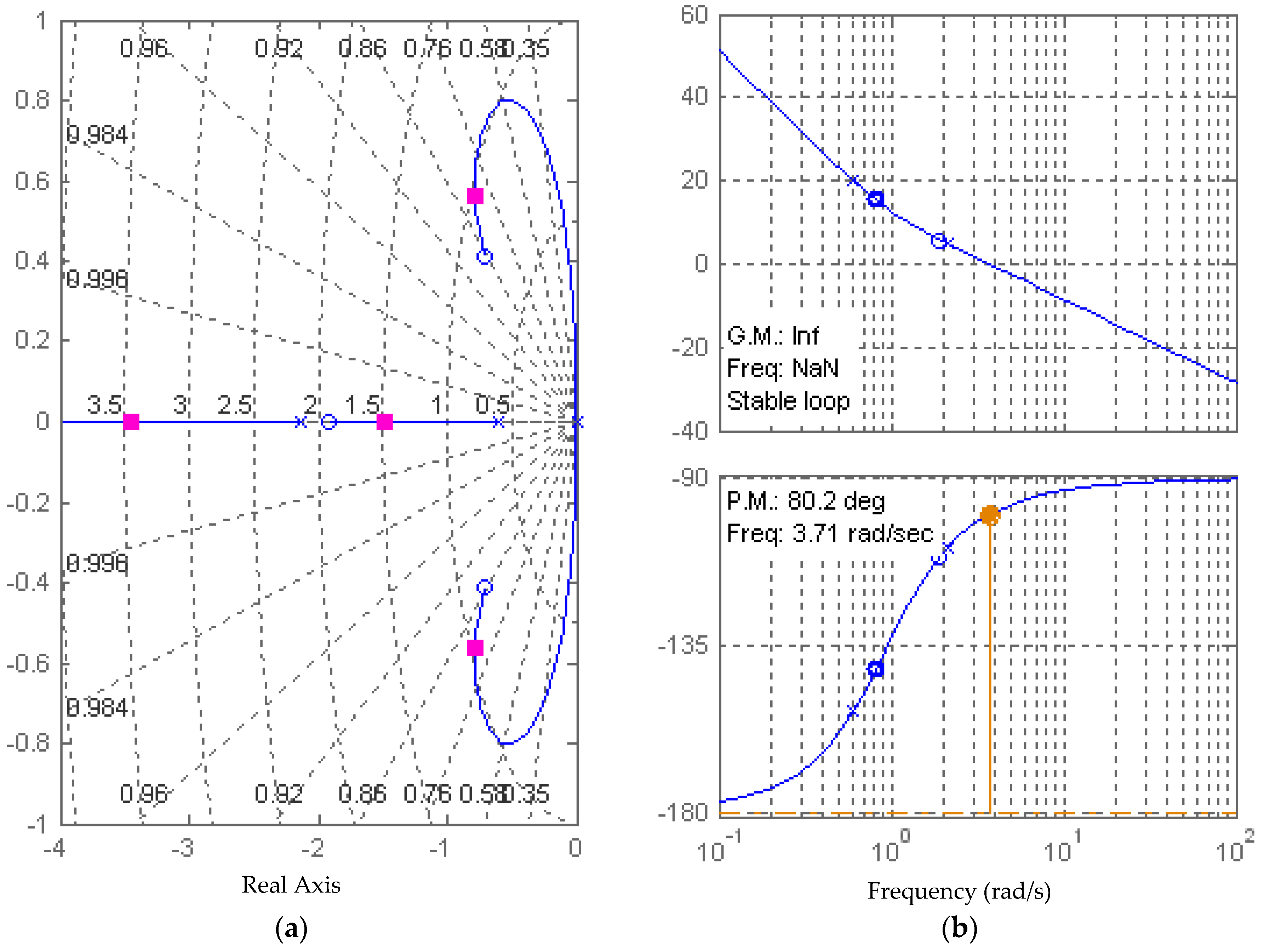
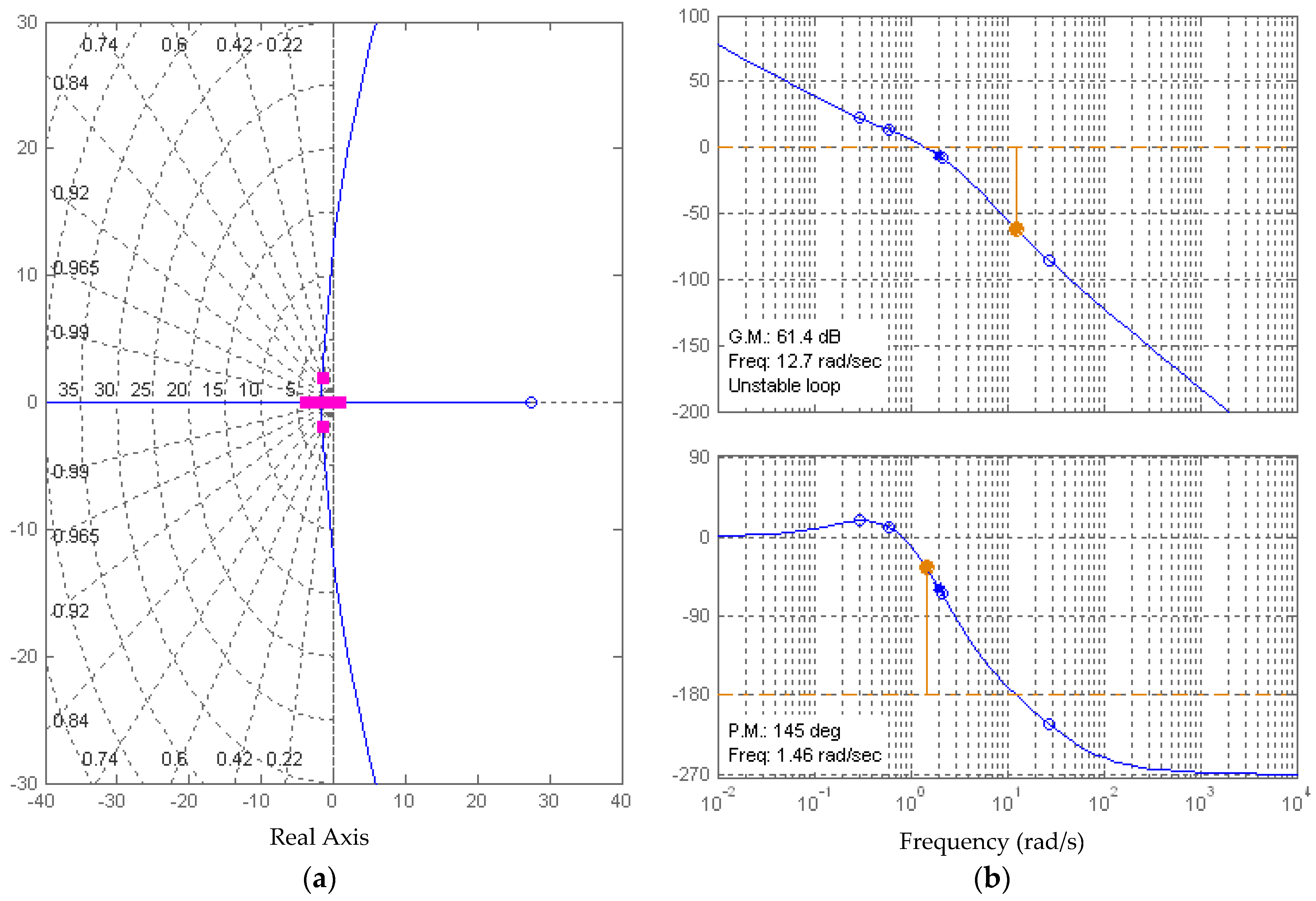
Figure 13.
The 61.4 degree gain margin and 145 degree phase margin using a reduced-order observer (both rule of thumb gains for half-controller tc = 0.5, and compensator with rule of thumb gains (tc = 1). (a) Root locus; and (b) Bode plot.
Figure 13.
The 61.4 degree gain margin and 145 degree phase margin using a reduced-order observer (both rule of thumb gains for half-controller tc = 0.5, and compensator with rule of thumb gains (tc = 1). (a) Root locus; and (b) Bode plot.
Figure 14.
Steady-state position error for various lateral underwater ocean currents.
Figure 14.
Steady-state position error for various lateral underwater ocean currents.
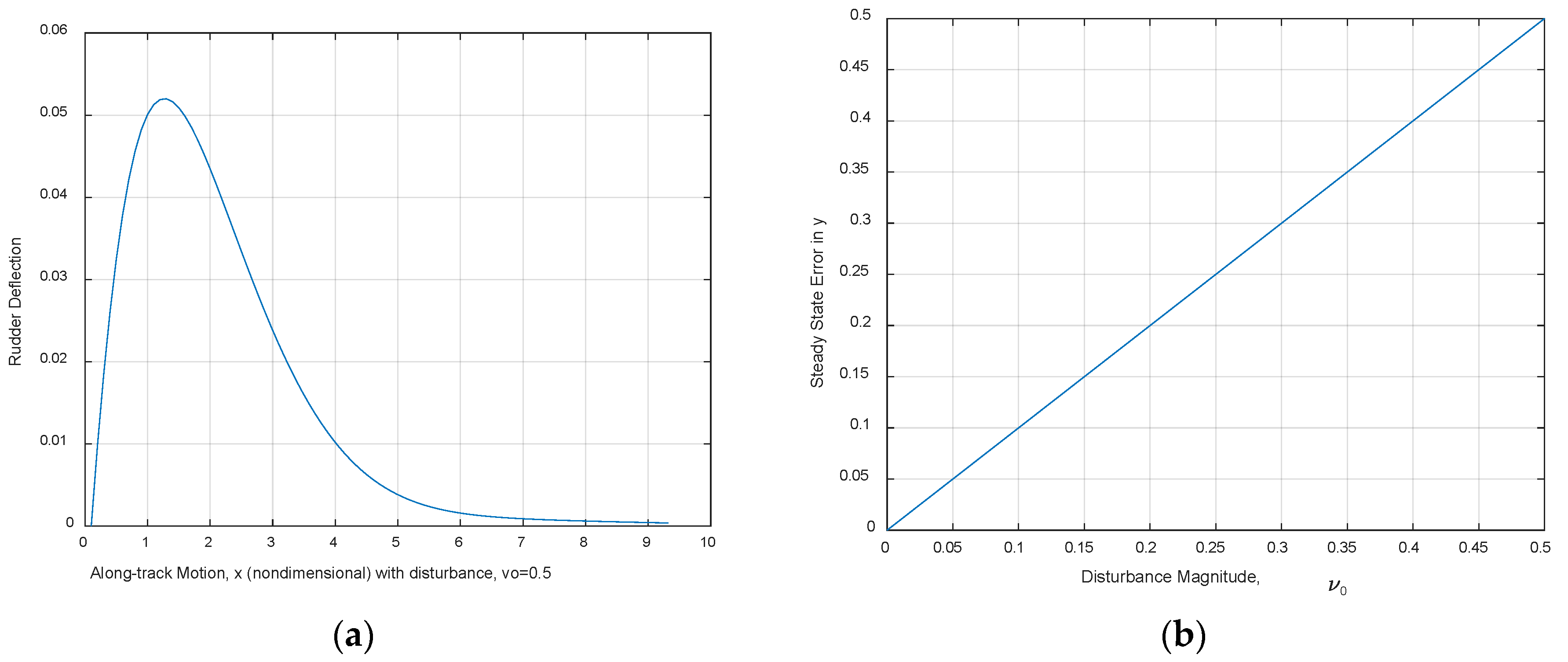
Figure 15.
Feedback alone is unable to counter the constant lateral underwater ocean currents. (a) Rudder deflection, ; and (b) steady state error vs. .
Figure 15.
Feedback alone is unable to counter the constant lateral underwater ocean currents. (a) Rudder deflection, ; and (b) steady state error vs. .
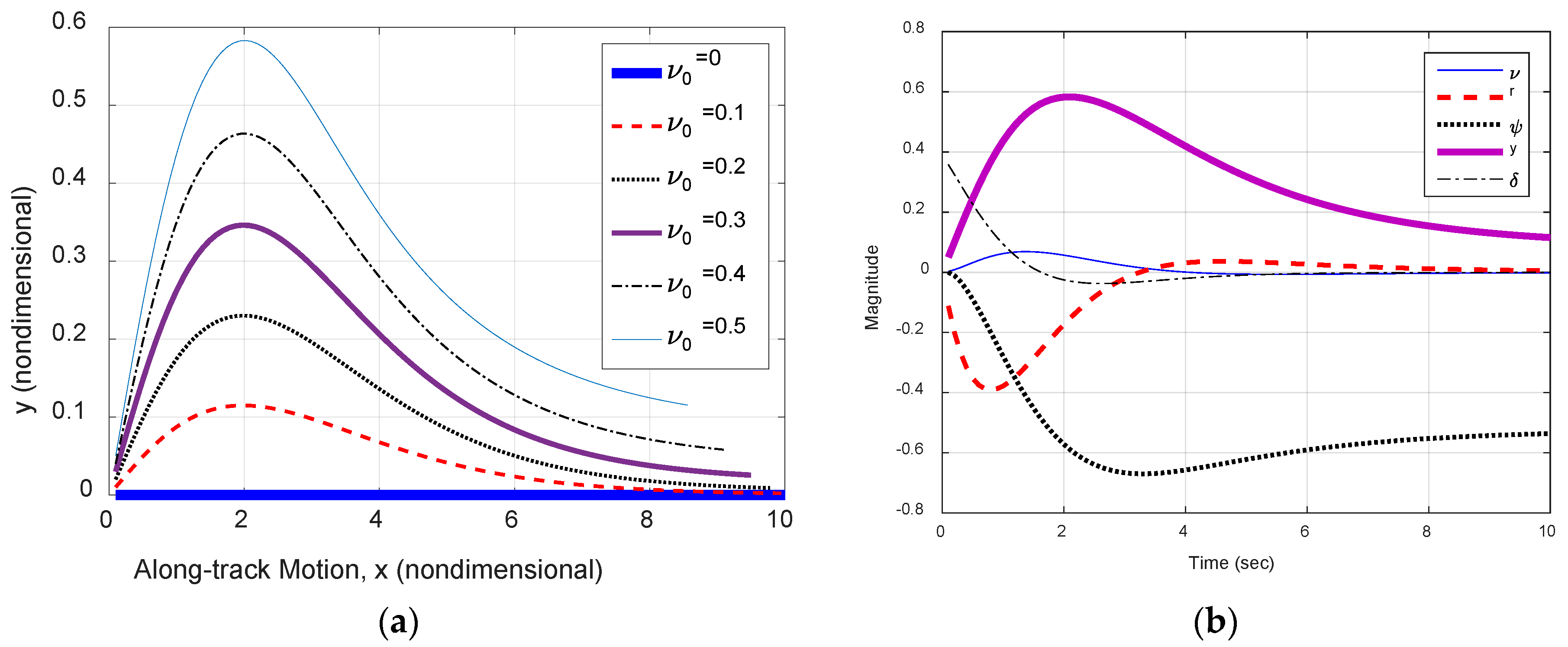
Figure 16.
Feed-forward element included to counter constant lateral underwater ocean currents. (a) Rudder deflection, ; and (b) all states when .
Figure 16.
Feed-forward element included to counter constant lateral underwater ocean currents. (a) Rudder deflection, ; and (b) all states when .
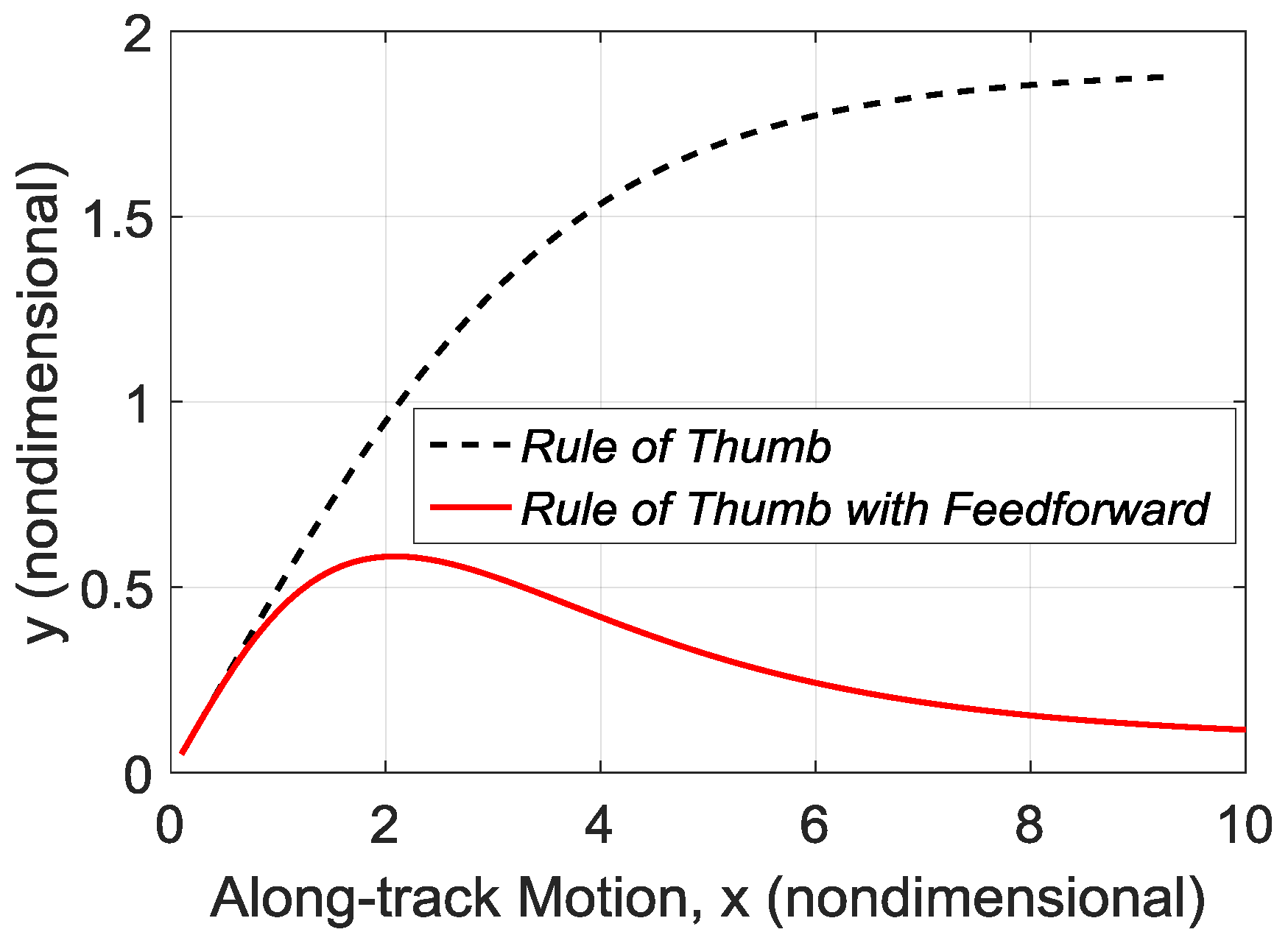
Figure 17.
Comparison: feedback control with and without feed-forward ().
Figure 17.
Comparison: feedback control with and without feed-forward ().
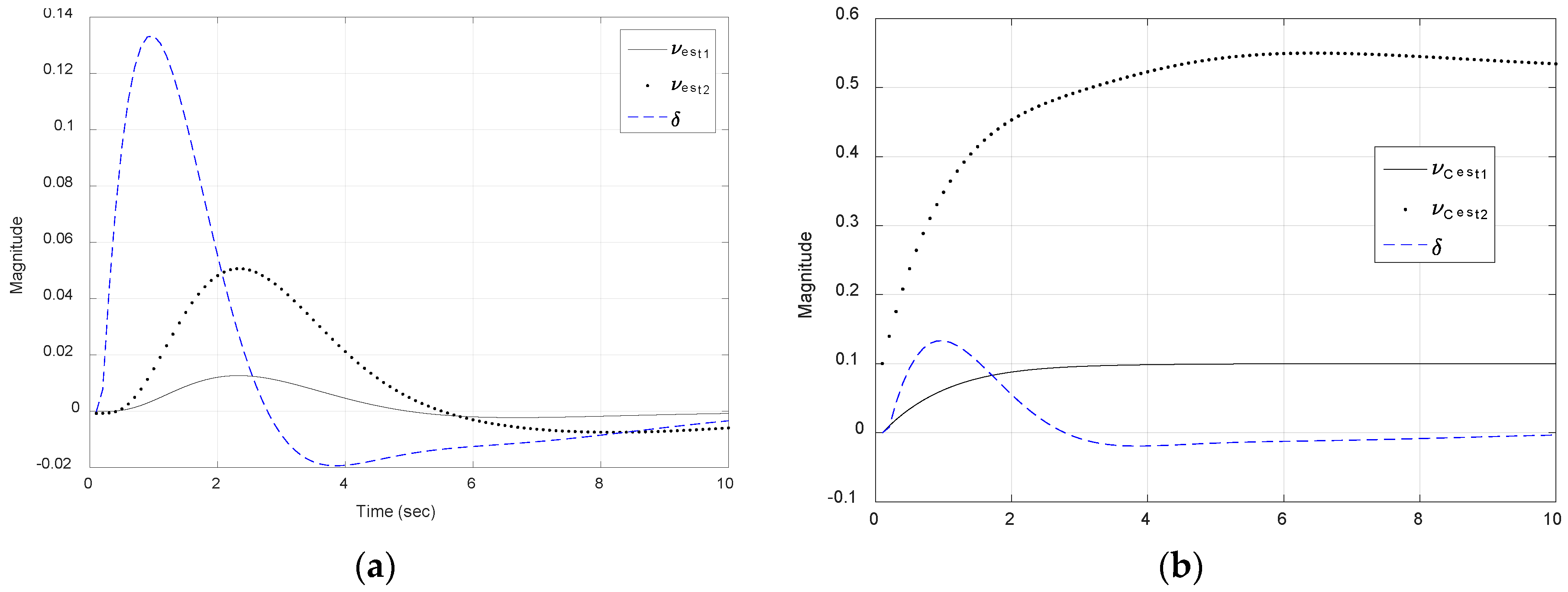
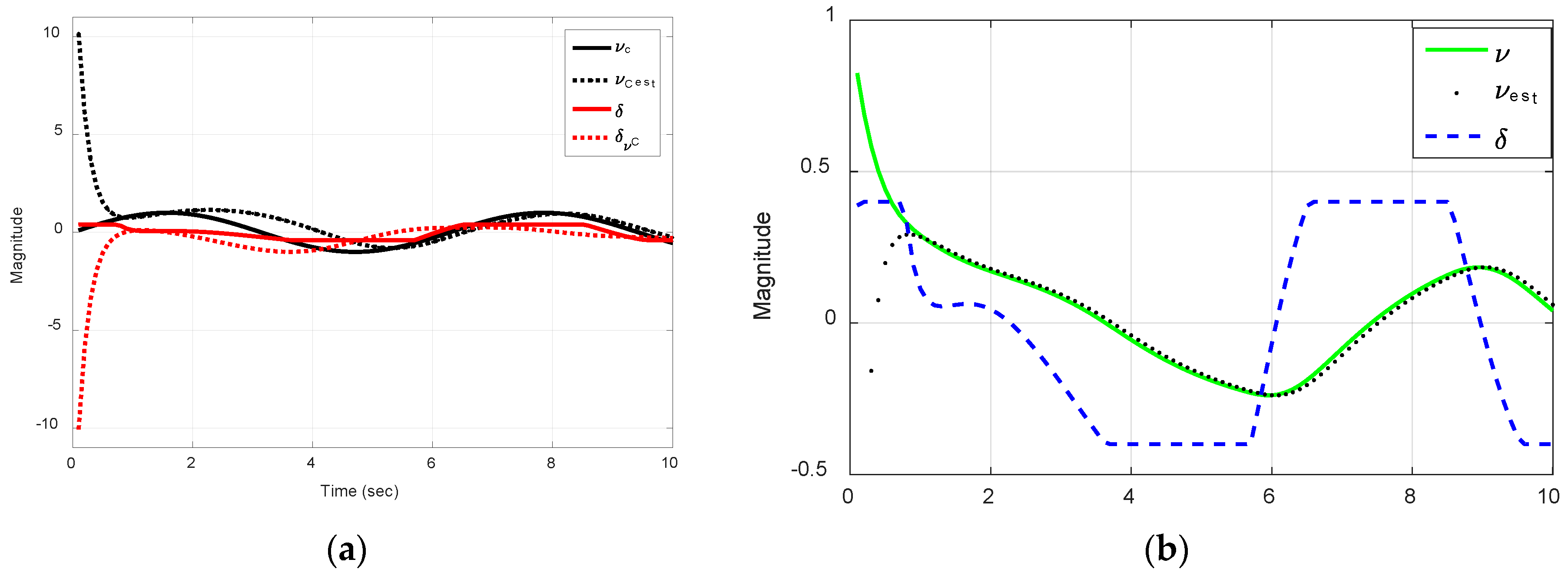
Figure 18.
Reduced-order observer state estimates versus time (seconds) for two disturbance currents , where is the rudder deflection using these estimates when the worst-case disturbance current is applied. (a) Sway velocity; (b) disturbance current; (c) lateral deviation (cross-track error); and (d) heading angle.
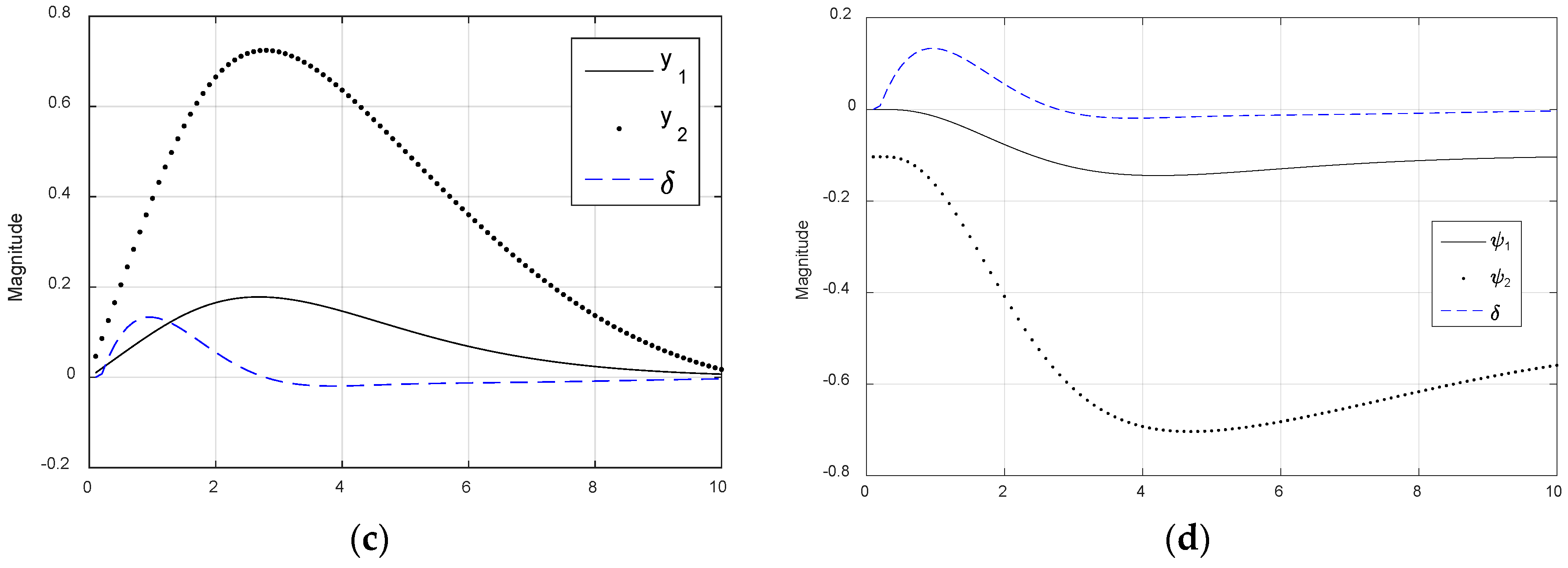
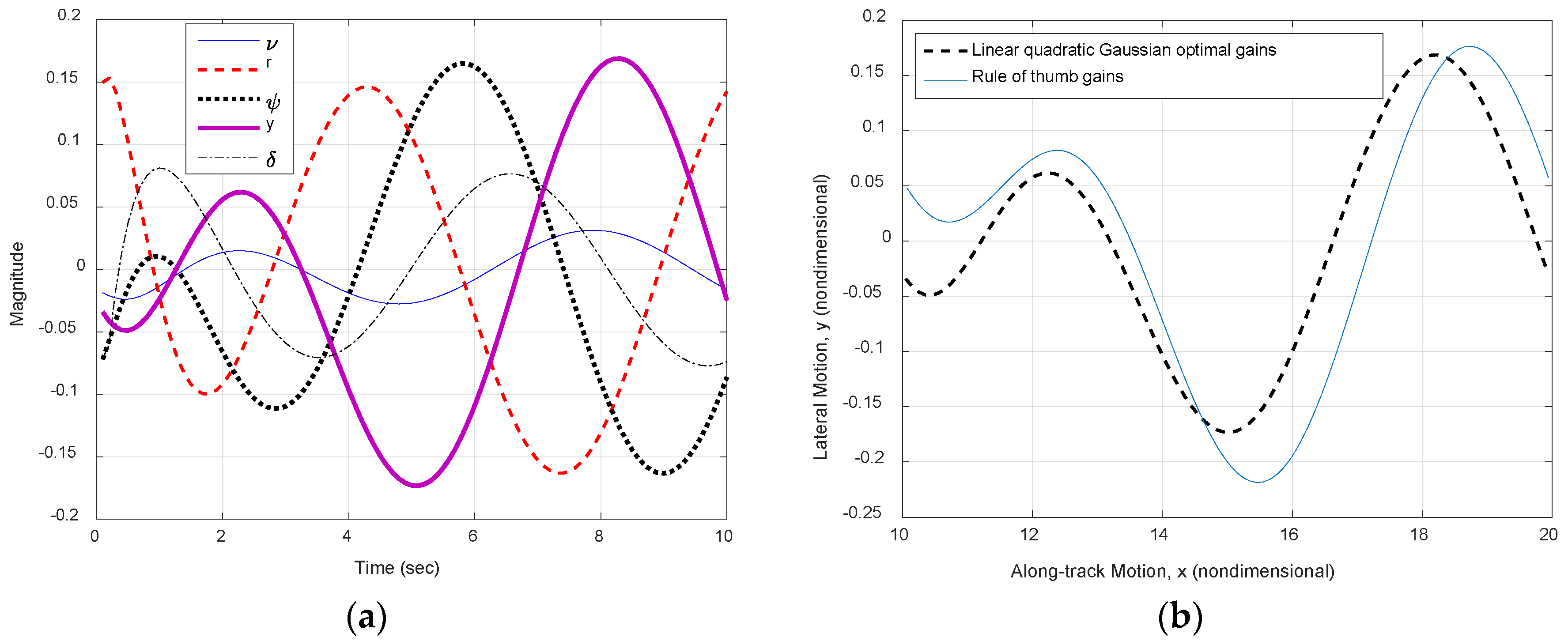
Figure 19.
Performance with disturbance estimation and command tracking using LQR and rule of thumb gains in a reduced-order observer, and command tracking to amidst a constant disturbance current . (a) States; and (b) trajectory.
Figure 19.
Performance with disturbance estimation and command tracking using LQR and rule of thumb gains in a reduced-order observer, and command tracking to amidst a constant disturbance current . (a) States; and (b) trajectory.
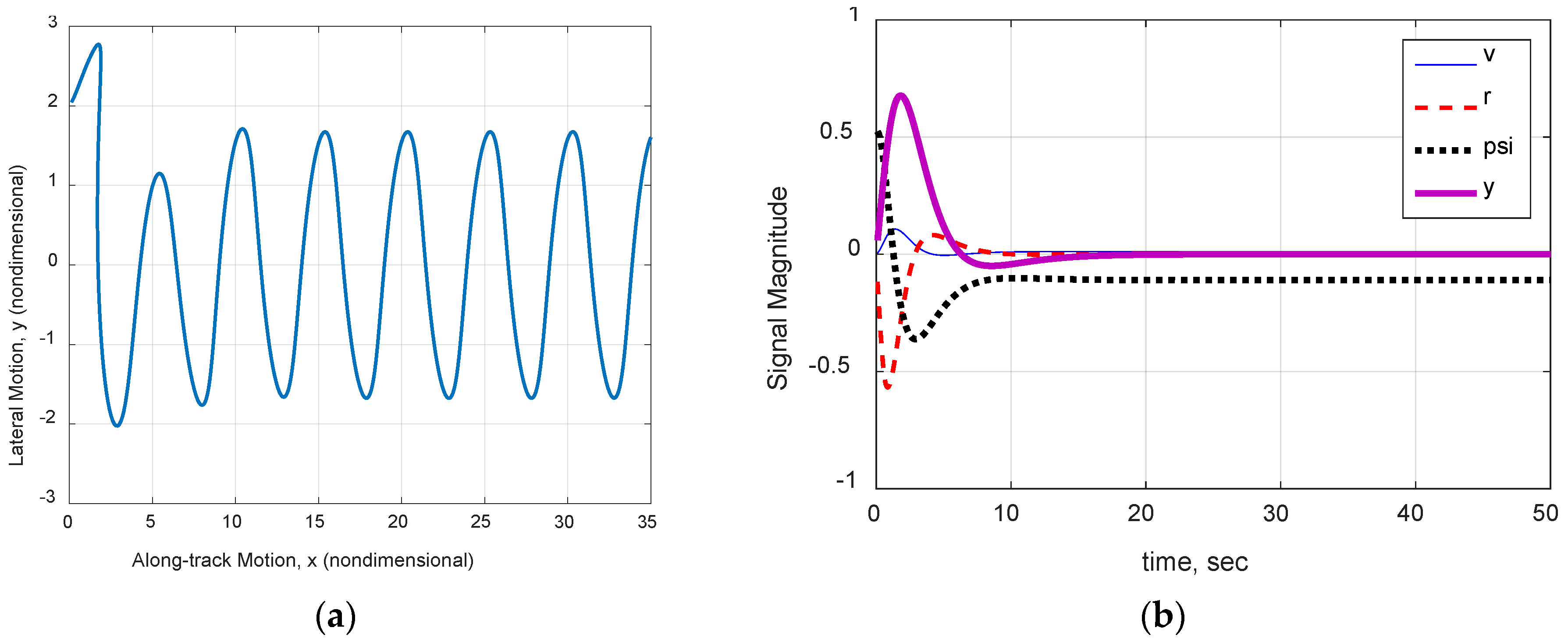
Figure 20.
Utilization of command tracking with reduced order observer, with command: and sinusoidal disturbance current , but no disturbance estimation or feed-forward. (a) All states vs. time (seconds); and (b) trajectory.
Figure 20.
Utilization of command tracking with reduced order observer, with command: and sinusoidal disturbance current , but no disturbance estimation or feed-forward. (a) All states vs. time (seconds); and (b) trajectory.
Figure 21.
Utilization of command tracking with reduced order observer, with command: ψ = −0.5, sinusoidal disturbance current , disturbance estimation, and feed-forward and rule of thumb gains.
Figure 21.
Utilization of command tracking with reduced order observer, with command: ψ = −0.5, sinusoidal disturbance current , disturbance estimation, and feed-forward and rule of thumb gains.
Figure 22.
Utilization of command tracking with reduced order observer, with command: ψ = −0.5 and sinusoidal disturbance current . (a) With disturbance estimation (and feed-forward), reduced order observer; and (b) with integral control, but no disturbance estimation or feed-forward.
Figure 22.
Utilization of command tracking with reduced order observer, with command: ψ = −0.5 and sinusoidal disturbance current . (a) With disturbance estimation (and feed-forward), reduced order observer; and (b) with integral control, but no disturbance estimation or feed-forward.
Figure 23.
Navigation through simulated field of 30 randomly placed mines in −0.5 m/s current with linear quadratic Gaussian PID controller and full-state observer.
Figure 23.
Navigation through simulated field of 30 randomly placed mines in −0.5 m/s current with linear quadratic Gaussian PID controller and full-state observer.
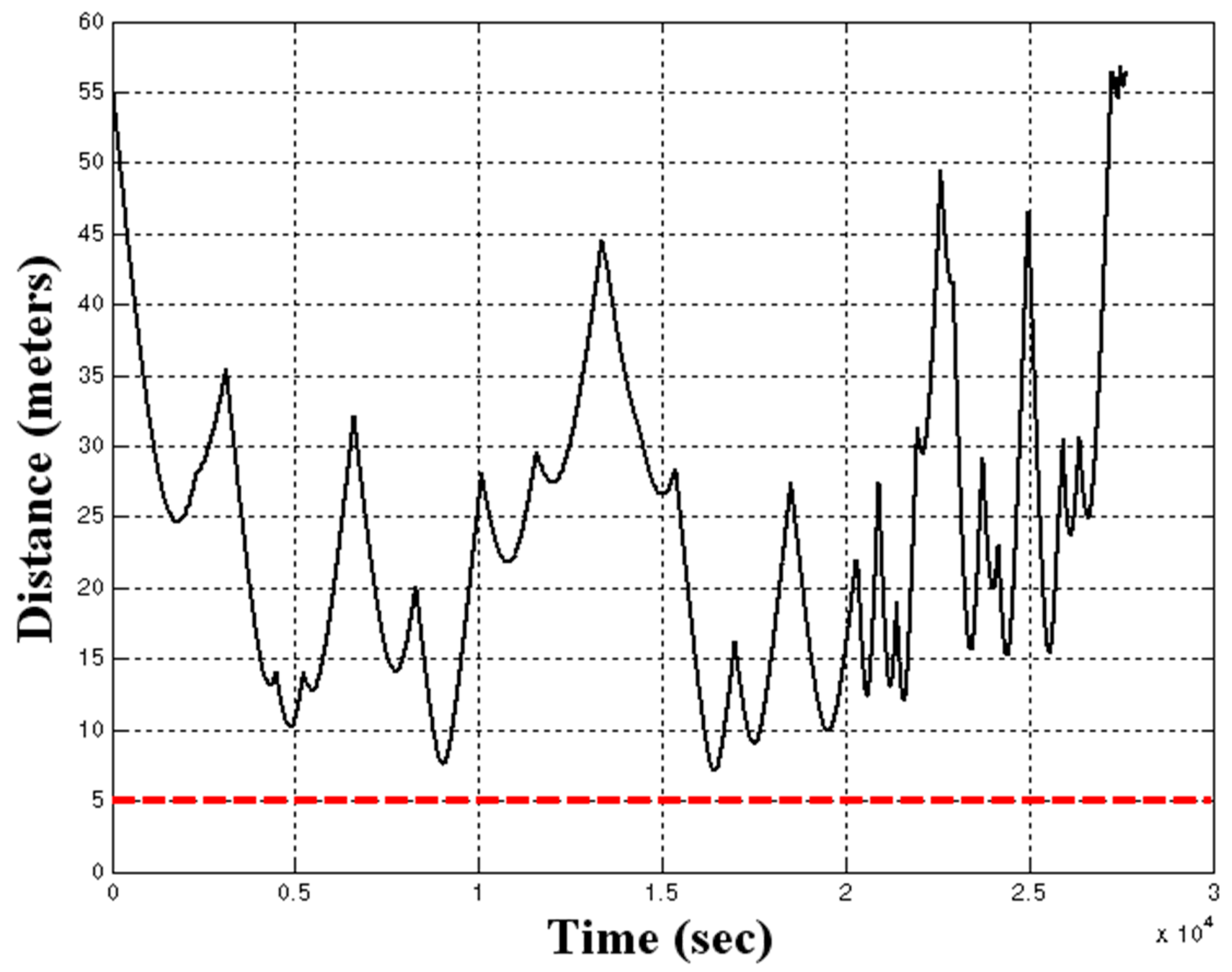
Figure 24.
Continuous distance (meters) to closest mine with Linear quadratic Gaussian optimized PID controller and full-state observer versus time (seconds).
Figure 24.
Continuous distance (meters) to closest mine with Linear quadratic Gaussian optimized PID controller and full-state observer versus time (seconds).
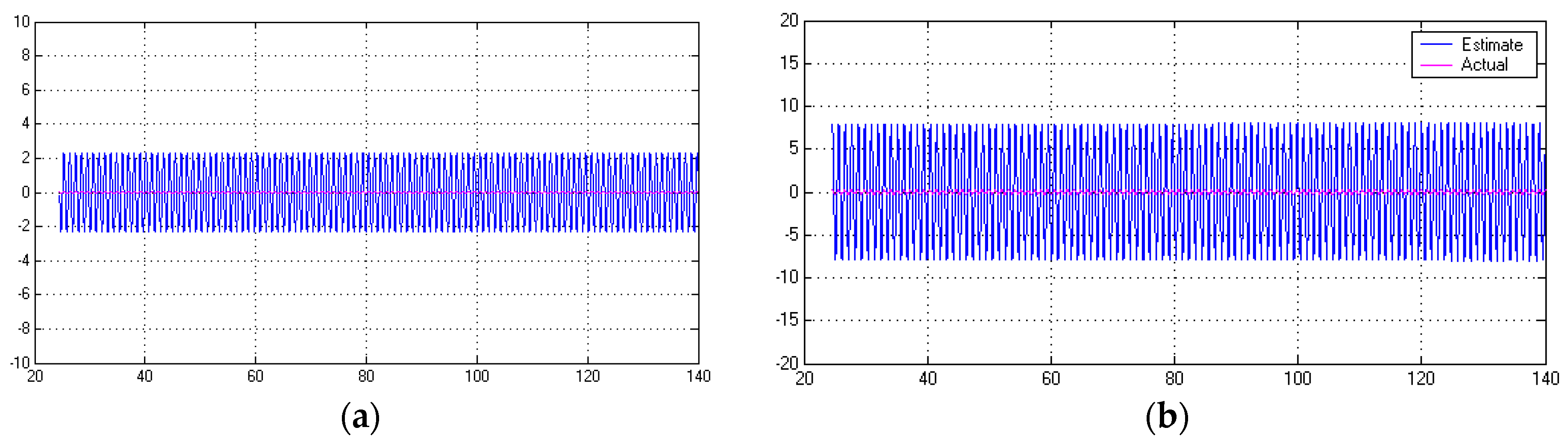
Figure 25.
Linear quadratic (Gaussian) optimal observer convergence with actual value in light-pink near zero, while estimates are depicted oscillating in blue. (a) State ; and (b) state .
Figure 25.
Linear quadratic (Gaussian) optimal observer convergence with actual value in light-pink near zero, while estimates are depicted oscillating in blue. (a) State ; and (b) state .
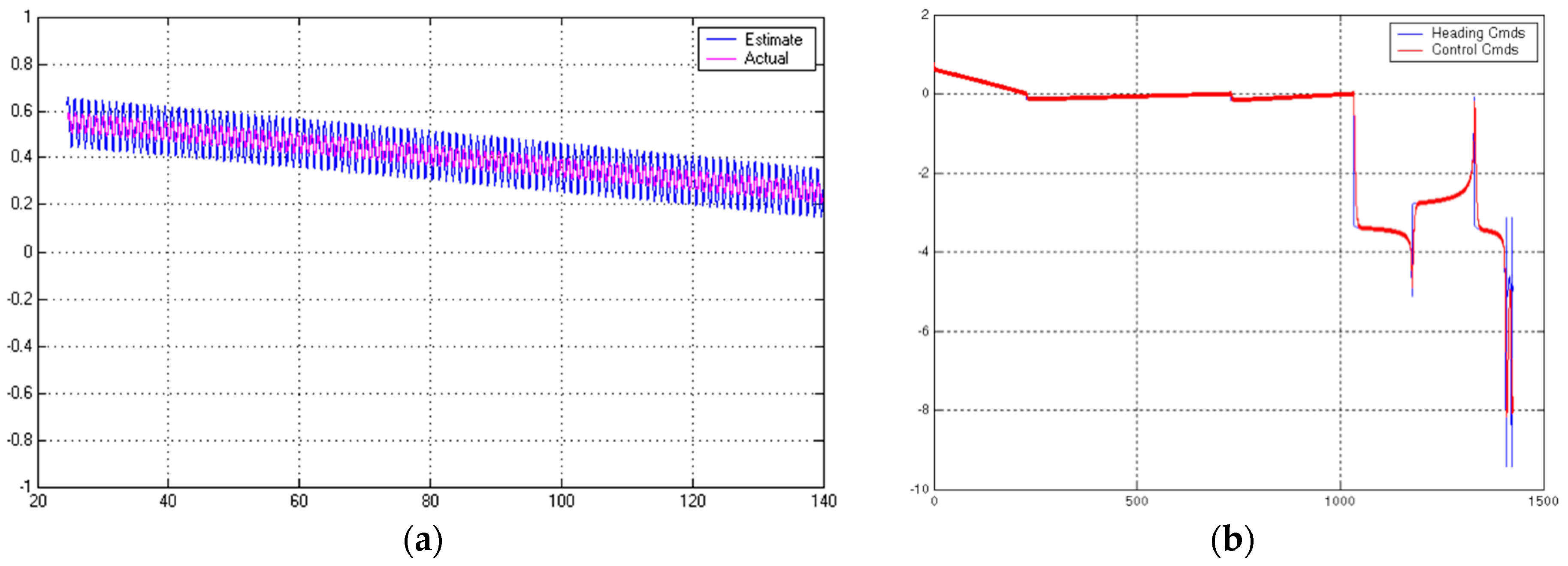
Figure 26.
Linear quadratic (Gaussian) optimal observer convergence. (a) State ; and (b) command tracking (radians) versus time (seconds).
Figure 26.
Linear quadratic (Gaussian) optimal observer convergence. (a) State ; and (b) command tracking (radians) versus time (seconds).
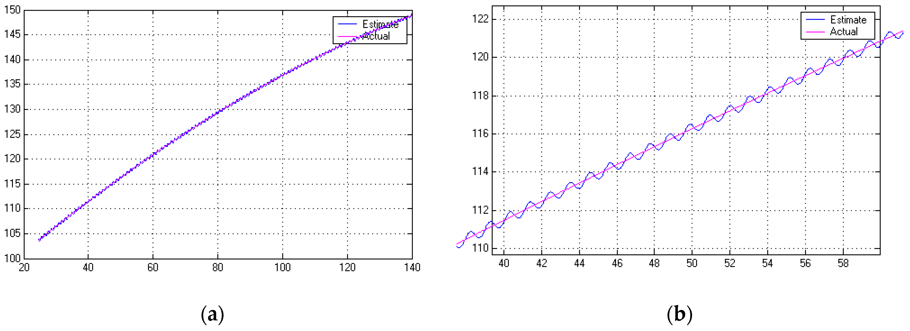
Figure 27.
Linear quadratic (Gaussian) optimal observer convergence of y; (a) State ; (b) State.
Figure 27.
Linear quadratic (Gaussian) optimal observer convergence of y; (a) State ; (b) State.
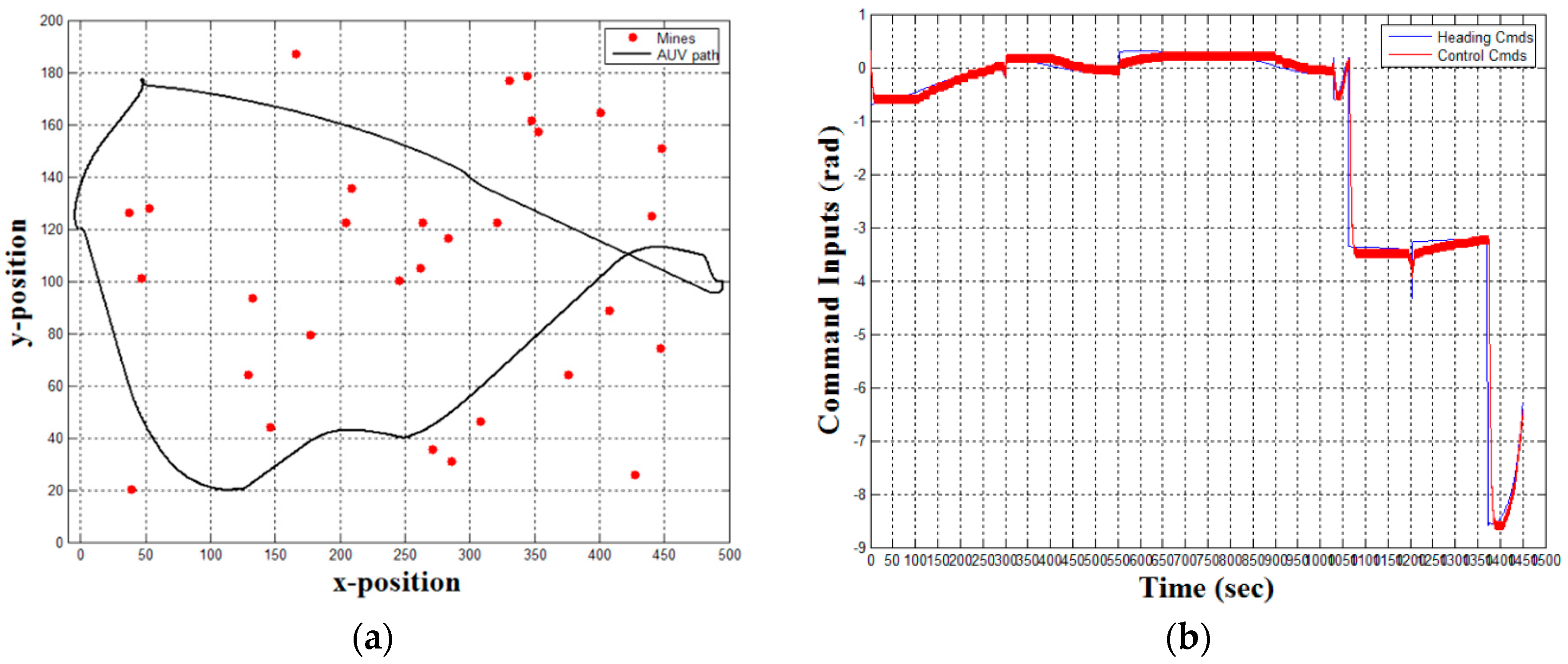
Figure 28.
Validation trajectory through simulated field of 30 randomly placed mines in −0.5 m/s current with linear quadratic Gaussian optimized PI controller and reduced-ordered observer. (a) Second trajectory (results validation); and (b) heading command tracking.
Figure 28.
Validation trajectory through simulated field of 30 randomly placed mines in −0.5 m/s current with linear quadratic Gaussian optimized PI controller and reduced-ordered observer. (a) Second trajectory (results validation); and (b) heading command tracking.
Table 1.
Comparison of simulation integration methodologies.
Table 1.
Comparison of simulation integration methodologies.
| Rudder Deflected | Euler: x-Distance 1 | Runge-Kutte: x-Distance 1 | Euler: y-Distance 1 | Runge-Kutte: y-Distance 1 |
|---|
| Bow | 6.5471 | 6.5469 | 6.8647 | 6.8646 |
| Stern | 3.1665 | 3.1665 | 3.5768 | 3.5768 |
| Both | 2.4546 | 2.4546 | 2.6567 | 2.6567 |
Table 2.
Gains for various time constants and also solution to linear quadratic optimization.
Table 2.
Gains for various time constants and also solution to linear quadratic optimization.
| Time Constant | | | | |
|---|
| 0.5 | −1.5135 | −1.7005 | −5.1508 | −3.22524 |
| 1 | 0.5070 | −0.3687 | −0.7157 | −0.1972 |
| 2 | 1.1248 | 0.2870 | −0.0906 | −0.0116 |
| LQR | −0.0939 | −1.2043 | −2.2138 | −1 |
Table 3.
Full-order observer gains designed by rule of thumb for various time constants as multiple of controller time constant, .
Table 3.
Full-order observer gains designed by rule of thumb for various time constants as multiple of controller time constant, .
| Multiple of the Controller Time Constant Used for the Observer | Observer Gain Matrix |
|---|
| 1 | |
| |
Table 4.
Observability matrix condition number for options to supplement the y measurement.
Table 4.
Observability matrix condition number for options to supplement the y measurement.
| Sensors Used to Measure States | Observability Matrix Condition Number 1 |
|---|
| and | 8.8456 |
| and | 21.1306 |
| and | 31.2919 |
Table 5.
Reduced-order observer gains designed by rule of thumb for various time constants as a multiple of the controller time constant, .
Table 5.
Reduced-order observer gains designed by rule of thumb for various time constants as a multiple of the controller time constant, .
| Multiple of the Controller Time Constant Used for Observer | Observer Gain Matrix |
|---|
| 1 | |
| |
| |


