Abstract
With the development of large-scale offshore projects, sea ice is a potential threat to the safety of offshore structures. The main forms of damage to bottom-fixed offshore structures under sea ice are crushing failure and bending failure. Referred to as the concept of seismic response spectrums, the design response spectrum of offshore structures induced by the crushing and bending ice failure is presented. Selecting the Bohai Sea in China as an example, the sea areas were divided into different ice zones due to the different sea ice parameters. Based on the crushing and bending failure power spectral densities of ice force, a large amount of ice force time-history samples are firstly generated for each ice zone. The time-history of the maximum responses of a series of single degree of freedom systems with different natural frequencies under the ice force are calculated and subsequently, a response spectrum curve is obtained. Finally, by fitting all the response spectrum curves from different samples, the design response spectrum is generated for each ice zone. The ice force influence coefficients for crushing and bending failure are obtained, which can be used to estimate the stochastic sea ice force acting on a structure conveniently in a static way. A comparison of the proposed response spectrum method with the Monte Carlo method by a numerical example shows good agreement.
1. Introduction
Freezing is a common natural phenomenon in winter at high latitudes of the earth. The ice force is a potential threat to bottom-fixed offshore structures due to its high magnitude and evident dynamic effects [1,2]. For instance, in 1969, the JZ20-2MSW platform was destroyed because of serious ice conditions in the Bohai Sea [3,4].
Many researchers have put their effort into the research of sea ice force and tried to present a more reasonable sea ice force model.
Su et al. [5] investigated the typical statistical characteristics of local ice loads based on the data from in-situ measurements. Neill [6] investigated the dynamic ice force on piers and piles. Torodd [7] studied model-based force and state estimation in experimental ice-induced vibrations. The feasibility and advantages of the ice-breaking cone were proven by the analytical results obtained by Ralston et al. [8] in the 1980s. Ordinary and serious ice conditions in the Bohai Sea were briefly presented by Zhang [9] and formulas for calculating the forces applied on offshore structures by ice were suggested.
From the above researches [5,6,7,8,9], the ice force is often regarded as a static load without considering its dynamic effects. In engineering design specifications, Nord [10], Qu [11], Barker [12], and Gravesen [13] conducted dynamic ice force experiments, respectively. Ice force acting on the Nordströmsgrund lighthouse was identified [10]. Qu [11] analyzed a random ice force for narrow conical structures through practical engineering experiments. Baker [12] and Gravesen [13] investigated the dynamic ice force on the offshore wind turbine, the dynamic characteristics of the structure under such loads were discovered.
Some dynamic ice force models have been recommended, while most of them are deterministic ones, such as the simplified dynamic ice force model presented by Kärnä and Qu [14]. Based on sea ice dynamics, Hunke et al. [15] established an elastic-viscous-plastic model. Li and Li [16] established a modified discrete element model for sea ice dynamics. Considering the redistribution process and the evolution of the ice thickness distribution, an idealized zero-dimensional model was presented by Godlovitch and Monahan [17]. Qu [18] proposed an ice dynamics model for narrow conical structures, which showed that ice-breaking cones were effective in reducing the ice force. On the other hand, the specific dynamic ice models have been developed based on local environmental conditions. Wang et al. [19] and Pedersen et al. [20] presented the proper sea ice dynamics models for the Gulf of Riga and the Greenland Sea, respectively. Besides, the dynamic and thermodynamic sea ice model for the subpolar regions was studied by Lu et al. [21]. However, sea ice breaking is a stochastic process in essence and it is usually difficult to simulate the action of ice force on offshore structures due to the low efficiency of the traditional random vibrations analysis method. Therefore, Shi [22], Zhi [23], and Ou [24] proposed the concept of sea ice force spectrums. Shi [22] recommended an ice force spectrum based on the displacement and strain responses of a single degree freedom structure, and more complicated structures were considered in the study of Zhi [23]. Ou [24] analyzed the characteristics of the random process of ice force and mechanism and established the relationship between spectral parameters and ice thickness.
The rupture forms of the sea ice can be mainly divided into several types, such as crushing failure, bending failure, and so on. Lee [25] investigated local ice load signals in ice-covered waters. Kim [26] discussed the assumptions behind rule-based ice loads of crushing failure. Through tests, the damage mechanism of sea ice was studied by Huang [27] in detail. The frequency of ice force under different ice failure modes and the occurrence probability of their magnitudes in full-scale had been studied by Suominen [28]. Zhang [29] studied the mechanism of ductile-brittle transition of sea ice damage and the influence of microcrack evolution on sea ice properties. Jones and Eylander [30] studied the ice force which acted on a vertical structure or inclined structure. Hayo et al. [31] investigated the ice-induced vibrations in the states of mixed crushing and buckling. Aksenov and Hibler [32] found that the icebreaking was highly irregular, and small cracks appeared around the broken area. Gagnon [33] established a numerical model for ice crushing failure. Sopper [34] performed a series of ice crushing tests to investigate the effects of external boundary conditions and geometric contact shapes under ice force.
In fact, ice force and the seismic effect have many similar characteristics, e.g., both of them are dynamic and stochastic with a specific frequency spectrum. Referred to as seismic design theory, the design response spectrums of sea ice force due to the crushing and bending failure are proposed. The novel method is simple and easy to analyze the response of bottom-fixed offshore structures subjected to ice.
Firstly, a single-degree of freedom (SDOF) model with different natural frequencies and damping is established to simulate different offshore structures subjected to ice force. Secondly, the crushing and bending failure power spectral densities (PSD) of the ice force, and the properties of ice are recommended. Thirdly, ice conditions in the Bohai Sea are selected as a typical investigated zone. A large amount of ice force time-history samples for crushing and bending failure are generated by applying the amplitude superposition method. Then, the maximum responses of SDOF structures with different natural frequencies subjected to each ice force time-history are obtained. The design response spectrums for both crushing and bending failure sea ice force are achieved. Finally, the numerical results validate the proposed method.
2. Analysis Model
Assume that the offshore structure can be simplified as a SDOF system, as shown in Figure 1, where m is the lumped mass; k is the shearing stiffness; and c is the damping coefficient; l1 and l2 indicate the heights above and under the sea level, respectively.
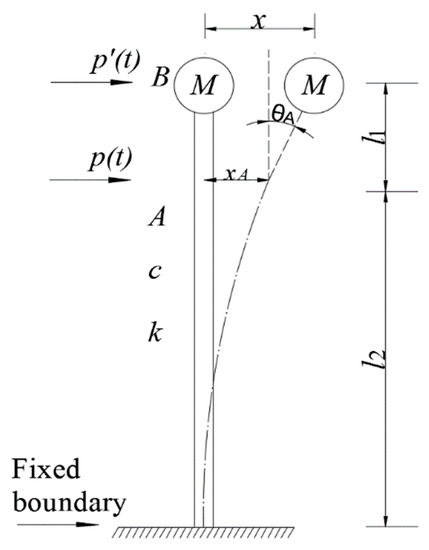
Figure 1.
Single-degree of freedom (SDOF) Model.
Since the system is excited by the ice force p(t) at the sea level (point A in Figure 1), rather than directly on the lumped mass (point B in Figure 1), the ice force should be replaced with an equivalent force p’(t) to establish the motion equation of the system. Neglecting the inertia force, the lateral displacement x and rotation θ at point A subjected to p(t) is:
where EI is the flexural stiffness of the cantilever beam. The displacement at point B is then:
Note that:
where k is the shear stiffness.
Equation (2) can be re-written as:
According to Equation (4), the displacement at point B induced by the equivalent ice force has to be equal to that raised by :
therefore,
The motion equation of the SDOF system subjected to ice force is then:
where , , and are the displacement, velocity, and acceleration of the SDOF system, respectively; and
where is the equivalent coefficient of the sea ice force.
3. PSDs of the Ice Force
3.1. Crushing Failure PSD
Based on a large amount of ice force practical measurement data of JZ9-3MDP in the Bohai Sea and the Norstromsgrund lighthouse, Kärnä and Qu [14,35] developed a crushing failure sea ice force power spectral density expression as follows:
where f (Hz) is the frequency of sea ice force; a and b are experimental parameters; is the ice velocity; and is the ice force standard deviation that is defined as:
where is the interaction strength of the dynamic ice with a mean value of 0.4 MPa; is the ice force amplitude when crushing failure happens; α is the comprehensive effect coefficient which lies between 0.4 and 0.7; is the ice compression strength; D is the loaded pile diameter of the structure; and h is the ice thickness.
3.2. Bending Failure PSD
In accordance with the ice load data collected on conical structures by a full-scale test in the Bohai Sea, Yue et al. [13,36] presented a bending failure sea ice force power spectral density as follows:
where is the ice force amplitude when bending failure occurs; is the ice force period. Their expressions are as follows:
where is ice bending strength; is the breaking length of the ice sheet; and τ is the ratio between breaking length and ice thickness with a value around 7.3.
3.3. Compression Strength and Bending Strength
Through the experiment, Vaudrey and Li [37,38] proposed formulas of the compression and bending strength for sea ice as follows:
where is the brine volume ratio of the sea ice,
where is the sea ice temperature; is the sea ice salinity.
4. Ice Force Parameters
As shown in Equations (9)–(15), there are four important parameters, including the temperature , salinity , thickness h, and velocity , which is related to the environment and affect the PSDs of the sea ice force. Essentially, they are all random variables and the way they are evaluated are explained in this section.
4.1. Ice Temperature and Salinity
Based on the different sea ice parameters, the Bohai Sea and the northern part of the Yellow Sea are divided into 21 zones by the China National Offshore Oil Production Research Centre and the National Marine Environmental Forecasting Center [39] as shown in Figure 2. Due to the scarcity of measured sea ice data in Zones 15–21, the ice parameters measured at a location within a certain zone is used to represent those of the zone. For instance, the data at Bayuquan Area represents that of Zone 21. The parameters of sea ice temperature and salinity corresponding to each ice zone in the Bohai Sea are listed in Table 1, which can be directly applied to Equations (12)–(15).
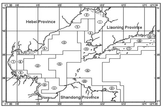
Figure 2.
The divided ice zones of the Bohai Sea.

Table 1.
Design values of sea ice temperature and salinity.
4.2. Probability Distributions of Ice Parameters
4.2.1. Probability Distributions of Ice Thickness and Ice Velocity
Based on a large amount of data recorded from the Bohai Sea and the northern Yellow Sea during the years of 1968–1998, researchers [35,36] indicated that the annual maximum thickness and velocity of the sea ice follow the Gumbel-logistic distribution, i.e., the joint distribution function of ice thickness and velocity can be expressed as:
where and are the marginal distribution of the random variable h and , respectively, which can be expressed as:
where and are the estimated values of the location of Gumbel distribution for ice thickness; and are the estimated values of scale parameters of Gumbel distribution for ice velocity:
In Equation (16), m (m ≥ 1) is the correlation parameter that can be estimated as:
where μ and σ denote the mean value and the standard deviation, respectively. It is obvious that when m = 1, h and are uncorrelated; while m→∞ indicates that h and are perfectly correlated.
An exceedance probability would be considered in the practical structural design to define the ice load-carrying capacity of the offshore structures. In this case, the ice thickness and velocity can be determined as:
where T is the recurrence period of the sea ice; is the inverse function of Equation (16), which represents a spatial curved surface for specified T. The possible sea ice thickness and velocity with exceedance probabilities of 63.2% and 2% for Zone 6 in the Bohai Sea are given in Figure 3, which corresponds to frequently met sea ice force and rarely met sea ice force, respectively.
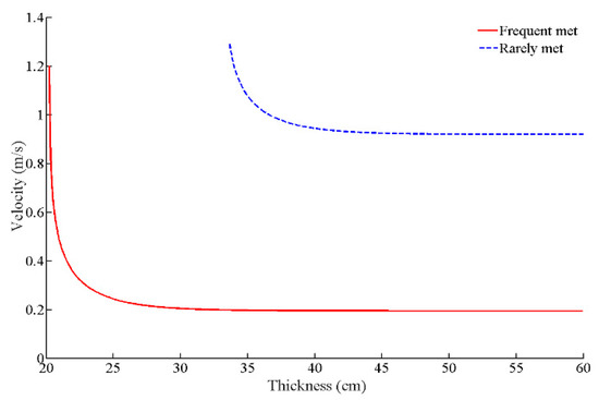
Figure 3.
The possible sea ice thickness and velocity.
Since the parameters mentioned previously are given, the PSDs of sea ice force given in Equations (9) and (11) can then be calculated as well. Typical PSDs for frequent met sea ice force are given in Figure 4, whereas other parameters are listed in Table 2.
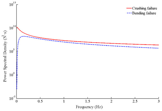
Figure 4.
The power spectral densities (PSDs) of ice damage.
Table 2.
Parameters for sea ice force PSDs.
4.2.2. Joint Probability Density Function of Ice Thickness and Ice Velocity
The joint probability density function is usually used to describe the correlation between two variables, which is equal to the derivative of ice thickness h and ice velocity Vice in Equation (16). Then, the joint probability density function of such random variables can be expressed as:
The ice zones in the Bohai Sea can be grouped into five groups through joint probability density, as listed in Table 3. The joint probability density of each zone in a group is close to each other. The independent variables x and y in the Equation (21) represent the thickness and velocity of ice, respectively. According to Equation (21), it can be discovered that the joint probability density increases with the increasing of ice thickness and ice velocity.
Table 3.
Joint probability density of ice thickness and ice velocity for each ice zone.
5. Proposed Sea Ice Response Spectrum
5.1. Generation of Ice Force Time-History Samples
For a zero-mean Gaussian Process with PSD, the amplitude superposition method is used to synthesize ice force time-history samples [40]:
where denotes the k-th frequency point; is the increment; and is the random phase that varies between . Two generated samples are given in Figure 5.
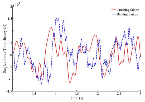
Figure 5.
Ice force time-history samples.
It is noted that in Equations (10) and (12), the parameter D is a structural geometrical parameter. In order to make the proposed method generally applicable, the related item should be extracted. Substituting Equation (10) into Equation (9), the ice force crushing failure PSD can be rewritten as:
According to Equation (21), the time-history due to ice force crushing failure can be generated as:
Similarly, the ice force bending failure PSD and time-history generated can be expressed as:
5.2. Response Spectrums for Each Ice Zone
The spectral characteristics of sea ice crushing damage and bending damage are similar to those of structure under earthquakes, which have abundant frequencies. Referred to as the earthquake response spectrum theory [41,42,43,44,45,46], a similar sea ice response spectrum theory is established in this section. According to Equations (7), (24), and (26), the motion equation of a SDOF system subjected to the ice forces can be expressed as:
where and are the feature coefficients of the offshore structure.
Equation (27) can also be rewritten as:
where ω is the natural frequency of the SDOF system; is the damping ratio. By means of Duhamel integral, its solution is:
where
For the sake of simplifying the dynamic problem expressed by Equation (7) to a static problem, the equivalent sea ice force acting on the SDOF system would be expressed as:
Ignore the tiny differences between and , and substitute Equation (30) into Equation (32), then:
The maximum absolute value of is:
where is the response spectrum of corresponding sea ice force time-history.
Normally speaking, a large amount of ice force time-history data based on in-situ measurements should be used as the excitation of the SDOF system to achieve the design response spectrum. Due to the scarity of the measured data, synthesized ice force time-histories have to be used. Considering the randomness of ice force due to the existence of phase φ in Equation (22), a large amount of ice force time-histories are synthesized for each zone. Based on Equation (34), a response spectrum corresponding to an ice force time-history can be calculated. Then, an envelope line covering the maximum response from the statistical data of each ice zone is fitted and normalized as the acceleration coefficient βmax. Acceleration response spectrums of crushing and bending failure are shown in Figure 6 and Figure 7 based on joint probability density of ice thickness and ice velocity in Section 4.
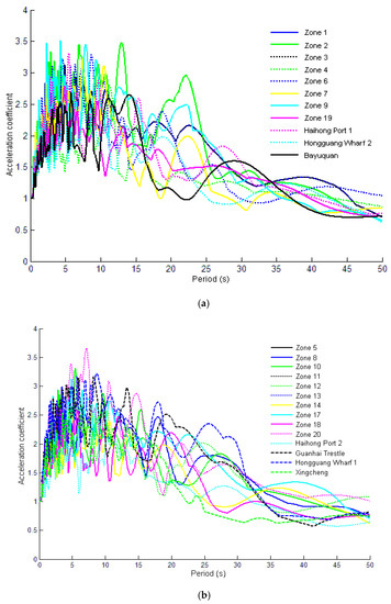
Figure 6.
Response spectrums of crushing failure. (a) In groups 1, 2; (b) in groups 3, 4, and 5.
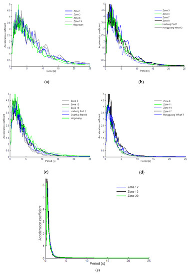
Figure 7.
Response spectrums of bending failure. (a) In group 1; (b) in group 2; (c) in group 3; (d) in group 4; (e) in group 5.
5.3. Design Response Spectrum for the Bohai Sea in China
Based on Equation (34), it is to be noted that the value of changes with the ice force time-history , the natural frequency ω, and the damping ratio of the SDOF system. By taking the maximum data of all response spectrum curves obtained from different sea ice time-history samples of each ice zone, and using the piecewise fitting method, the design response spectrum of the sea ice force is achieved, which is shown in Figure 8 and denoted by , where , , , and are the parameters related to structural damping.
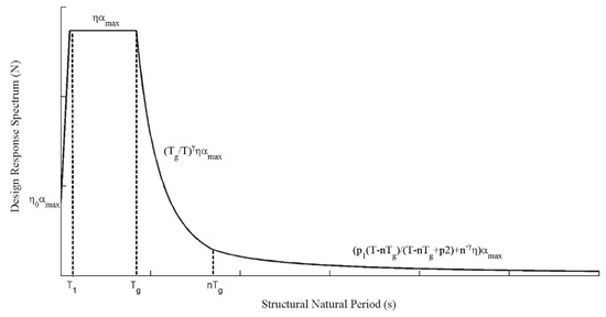
Figure 8.
Design Response Spectrum.
Selecting Zone 6 as an example and taking numerical fitting, the design spectrum parameters for crushing failure sea ice force can be obtained:
Additionally for bending failure sea ice force:
Other fitting parameters combined ice velocity and thickness of exceedance probabilities for Zone 6 in the Bohai Sea are given in Table 4 and Table 5.
Table 4.
Fitting parameters for Zone 6.
Table 5.
The value of αmax for Zone 6.
By replacing and by and in Equation (34), respectively, the stochastic sea ice force acting on a structure can then be estimated easily in a static way as:
Hence, the proposed response spectrum method can be applied as follows [47]:
Step 1, Calculate η0, η, γ, p1 and p2 based on Equations (35)–(40).
Step 3, Obtain the static sea ice force using Equation (41).
Step 4, Compute the concerned structural response.
6. Numerical Example
In this section, selecting Zone 6 as an example, the proposed method is verified by comparing the results derived from the Monte-Carlo simulation. Taking the SDOF offshore structure as the research object, whose lumped mass is 106 kg and damping ratio is 0.02, and which natural period varies with the changing stiffness. Assume that the loaded pile diameter of the structure is 2.7 m and the heights above and under the sea level are 20 m and 80 m, respectively. The displacements excited by crushing and bending failure sea ice force are studied, respectively.
In the Monte-Carlo simulation, 200 time-history samples are generated for both crushing and bending failure sea ice force. Based on the Monte-Carlo method and the ice force response method, Figure 9 and Figure 10 show the displacements of the offshore structure with different structural natural periods subjected to crushing and bending failure sea ice force. It can be seen that the results obtained from the two methods display a manifested same trend.
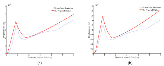
Figure 9.
The displacements subjected to frequent met sea ice force. (a) Sea ice crushing failure; (b) sea ice bending failure.
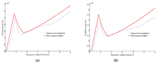
Figure 10.
The displacements subjected to rarely met sea ice force. (a) Sea ice crushing failure; (b) sea ice bending failure.
From Figure 9 and Figure 10, the displacement induced by ice bending failure is less than that by ice crushing failure. Meanwhile, it can be seen that the displacement under rarely met sea ice force is greater than that under frequent met sea ice force. Generally speaking, the proposed method provides an upper limit.
As shown in Figure 9 and Figure 10, for the offshore structures with natural periods in the interval of [0,T1], which have either large rigidity or light-weight, the response such as displacement will increase with the increasing structural natural periods. For the offshore structure with natural period in the interval of (T1, nTg], the response will increase remarkably. It is clear that resonance will occur if the structure natural period is close to Tg. When T is larger than nTg, the structural displacement will increase with the increase of structural natural periods due to the decreasing structural stiffness.
The computing time of the example required for the proposed method is only 0.04 s while, that for the Monte-Carlo simulation is 7537.6 s. It is obvious that the proposed method is not only easy to calculate but also matches the needs in engineering and has common applicability.
7. Conclusions
Referred to as the earthquake response spectrum theory, a new design idea to determine the maximum response of offshore structures subjected to ice forces is suggested.
(1) Considering the randomness of ice force and the complexity of structures, the theory of response spectrum suitable for offshore structures subjected to crushing and bending failure sea ice forces is established.
(2) Selecting Zone 6 in the Bohai Sea, dynamic analysis of SDOF structures subjected to synthesized ice force time-histories is performed. Then, the design response spectrums for fixed offshore structures subjected to ice forces induced by crushing and bending failure are proposed, respectively.
(3) Compared with results from the Monte-Carlo simulation and the proposed method, the proposed method is validated. Additionally, the proposed method provides an upper limit of offshore structural response subjected to ice force.
(4) For the offshore structure with a natural period in the range of (T1, nTg], the response under ice force will increase remarkably. The maximum response will occur when the structure natural period is close to Tg.
Author Contributions
Y.L. and Y.Z.: Writing and data collection; X.L.: Data analysis, interpretation and revising; Y.L. and Y.Z.: methodology and software; Y.L.: Numerical analysis and revising. All the authors contributed to the first draft and final version of the paper.
Funding
This study was supported by the National Natural Science Foundation of China (Grant No. 51879040).
Conflicts of Interest
The authors declare no conflict of interest.
Nomenclature:
| Parameter | Nomenclature | Parameter | Nomenclature |
| m | lumped mass of a single-degree of freedom system (SDOFS) | p’(t) | an equivalent force of SDOFS |
| k | shearing stiffness of SDOFS | ice force amplitude when crushing failure happens | |
| c | damping coefficient of SDOFS | ice force amplitude when bending failure happens | |
| h | sea ice thickness | the marginal distribution | |
| heights above and under the sea level | ice force | ||
| x | lateral displacement of point A | the ice force period | |
| θ | rotation of point A | T | recurrence period of the sea ice |
| λ | the equivalent coefficient of the sea ice force | sea ice temperature | |
| f | sea ice force frequency | sea ice salinity | |
| the k-th frequency point | random phase that varies between [0, 2π) | ||
| the increment frequency | ω | natural frequency of the SDOFS | |
| ice force standard deviation | damping ratio of offshore structure | ||
| ice compression strength | the breaking length of ice sheet | ||
| ice flexural strength | a parameter that related to structural damping | ||
| sea ice velocity | a parameter that related to structural damping | ||
| D | loaded pile diameter of the structure | a parameter that related to structural damping | |
| τ | the ratio between breaking length and ice thickness | a parameter that related to structural damping | |
| power spectral densities | a parameter that related to structural damping | ||
| the response spectrum of corresponding sea ice force time history | the interaction strength of the dynamic ice with a mean value of 0.4 | ||
| α | ice force of design response spectrum for Bohai Sea | a b | experimental parameters |
References
- Kotilainen, M. Predicting ice-induced load amplitudes on ship bow conditional on ice thickness and ship speed in the Baltic Sea. Cold Reg. Sci. Technol. 2017, 135, 116–126. [Google Scholar] [CrossRef]
- Ranta, J.; Polojärvi, A.; Tuhkuri, J. The statistical analysis of peak ice loads in a simulated ice-structure interaction process. Cold Reg. Sci. Technol. 2017, 133, 46–55. [Google Scholar] [CrossRef]
- Li, W.; Huang, Y.; Tian, Y. Experimental study of the ice loads on multi-piled oil piers in Bohai Sea. Mar. Struct. 2017, 56, 1–23. [Google Scholar] [CrossRef]
- Shun, Y.; Yue, O.J.; Bi, X.J. Probability distribution of sea ice fatigue parameters in JZ20-2 sea area of the Liaodong Bay. Ocean Eng. 2002, 20, 39–44. [Google Scholar]
- Su, B.; Riska, K.; Moan, T. Numerical simulation of local ice loads in uniform and randomly varying ice conditions. Cold Reg. Sci. Technol. 2011, 65, 145–159. [Google Scholar] [CrossRef]
- Neill, R.C. Dynamic ice forces on piers and piles. An assessment of design guidelines in the light of recent research. Can. J. Civ. Eng. 1976, 3, 305–341. [Google Scholar] [CrossRef]
- Nord, T.S. Model-based force and state estimation in experimental ice-induced vibrations by means of Kalman filtering. Cold Reg. Sci. Technol. 2015, 111, 13–26. [Google Scholar] [CrossRef]
- Ralston, T.D.; Riska, K. Ice force design considerations for conical offshore structures. Force 1977, 2. [Google Scholar]
- Zhang, F.J. The significance of sea ice forces in the design of ocean engineering structures in the Bohai Sea. Ocean Eng. 1987, 5, 59–65. [Google Scholar]
- Nord, T.S.; Øiseth, O.; Lourens, E. Ice force identification on the Nordströmsgrund lighthouse. Comput. Struct. 2016, 169, 24–39. [Google Scholar] [CrossRef]
- Qu, Y. Ice force spectrum on narrow conical structures. Cold Reg. Sci. Technol. 2007, 49, 161–169. [Google Scholar]
- Barker, A. Ice loading on Danish wind turbines. Cold Reg. Sci. Technol. 2005, 41, 1–23. [Google Scholar] [CrossRef]
- Gravesen, H. Ice loading on Danish wind turbines: Part 2. Analyses of dynamic model test results. Cold Reg. Sci. Technol. 2005, 41, 25–47. [Google Scholar] [CrossRef]
- Kärnä, T.; Qu, Y. A New Spectral Method for Modeling Dynamic Ice Actions. In Proceedings of the 23rd International Conference on Offshore Mechanics and Arctic Engineering, Vancouver, BC, Canada, 20–25 June 2004. [Google Scholar]
- Hunke, E.C.; Dukowicz, J. An elastic-viscous-plastic model for sea ice dynamics. J. Phys. Oceanogr. 1997, 27, 1849–1867. [Google Scholar] [CrossRef]
- Li, B.H.; Li, H. A modified discrete element model for sea ice dynamics. Acta Oceanol. Sin. 2014, 33, 56–63. [Google Scholar] [CrossRef]
- Godlovitch, D.; Monahan, A. An idealised stochastic model of sea ice thickness dynamics. Cold Reg. Sci. Technol. 2012, 78, 14–30. [Google Scholar] [CrossRef]
- Qu, Y. A random ice force model for narrow conical structures. Cold Reg. Sci. Technol. 2006, 45, 148–157. [Google Scholar]
- Wang, K.; Leppäranta, M. A sea ice dynamics model for the Gulf of Riga. Proc. Est. Acad. Sci. Eng. 2003, 9, 107–125. [Google Scholar]
- Pedersen, L.T.; Coon, M.D. A sea ice model for the marginal ice zone with an application to the Greenland Sea. J. Geophys. Res. Ocean. 2004, 109, 1–8. [Google Scholar] [CrossRef]
- Lu, Q.M.; Larsen, J.; Tryde, P. A dynamic and thermodynamic sea ice model for subpolar regions. J. Geophys. Res. Ocean. 1990, 95, 13433–13457. [Google Scholar] [CrossRef]
- Shi, Q.Z. Dynamics of sea ice and spectrums of ice force. China Ocean Eng. 1994, 16, 107–111. [Google Scholar]
- Zhi, H. Identification of random ice force spectra of offshore platforms. Ocean Eng. 2000, 18, 14–17. [Google Scholar]
- Ou, J.P. A stochastic process model of ice pressure on a Bohai jacket platform and its parameters. Acta Oceanol. Sin. 1998, 20, 111–118. [Google Scholar]
- Lee, J.H. Characteristics analysis of local ice load signals in ice-covered waters. Int. J. Nav. Archit. Ocean Eng. 2016, 8, 66–72. [Google Scholar] [CrossRef]
- Kim, E.; Amdahl, J. Discussion of assumptions behind rule-based ice loads due to crushing. Ocean Eng. 2016, 119, 249–261. [Google Scholar] [CrossRef]
- Huang, Y. Experimental study on ice destruction mechanism. Ship Build. China 2003, 44, 380–386. [Google Scholar]
- Suominen, M. Influence of load length on short-term ice load statistics in full-scale. Mar. Struct. 2017, 52, 153–172. [Google Scholar] [CrossRef]
- Zhang, X. Steady Vibration of Ice-Induced Vertical Structure. Master’s Thesis, Dalian University of Technology, Dalian, China, 2002. [Google Scholar]
- Jones, K.; Eylander, J. Vertical variation of ice loads from freezing rain. Cold Reg. Sci. Technol. 2017, 143, 126–136. [Google Scholar] [CrossRef]
- Hendrikse, H.; Metrikine, A. Ice-induced vibrations and ice buckling. Cold Reg. Sci. Technol. 2016, 131, 129–141. [Google Scholar] [CrossRef]
- Aksenov, Y.; Hibler, W.D. Failure Propagation Effects in an Anisotropic Sea Ice Dynamics Model. In Proceedings of the IUTAM Symposium on Scaling Laws in Ice Mechanics and Ice Dynamics Fairbanks, Alaska, USA, 13–16 June 2000; Volume 94, pp. 363–372. [Google Scholar]
- Gagnon, R.E. A numerical model of ice crushing using a foam analogue. Cold Reg. Sci. Technol. 2011, 65, 335–350. [Google Scholar] [CrossRef]
- Sopper, R. The influence of water, snow and granular ice on ice failure processes, ice load magnitude and process pressure. Cold Reg. Sci. Technol. 2017, 139, 51–64. [Google Scholar] [CrossRef]
- Qu, Y. Random Ice Load Analysis on Offshore Structures Based on Field Tests. Ph.D. Thesis, Dalian University of Technology, Dalian, China, 2006. [Google Scholar]
- Yue, Q.J. Fatigue-Life Analysis of Ice Resistant Platforms. Eng. Mech. 2017, 24, 159–164. [Google Scholar]
- Vaudrey. Elastic Property Studies on Compressive and Flexural Sea Ice Specimens; Civil Engeneering Lab: Port Hueneme, CA, USA, 1975; Volume 12, pp. 1–16. [Google Scholar]
- Li, Z.J. Preliminary statistics on the elements involved in sea ice in Liaodong Bay. Ocean Eng. 1992, 10, 72–78. [Google Scholar]
- Regulations for Offshore Ice Condition and Application in China Sea, in Q/HSn 3000-2002; The China National Offshore Oil Production Research Centre and the National Marine Environmental Forecasting Center: China, 2002; p. 34.
- Qu, Y.; Bi, X. Ice-induced Jacket Structure Vibrationss in Bohai Sea. J. Cold Reg. Eng. 2017, 14, 81–92. [Google Scholar]
- Bani-Hani, K.A.; Malkawi, A.I. A Multi-step approach to generate response-spectrum-compatible artificial earthquake accelerograms. Soil Dyn. Earthq. Eng. 2017, 97, 117–132. [Google Scholar] [CrossRef]
- Leppäranta, M. A treatise on frequency spectrum of drift ice velocity. Cold Reg. Sci. Technol. 2012, 76, 83–91. [Google Scholar] [CrossRef]
- Cacciola, P.; Amico, L.D.; Zentner, I. New insights in the analysis of the structural response to response-spectrum-compatible accelerograms. Eng. Struct. 2014, 78, 3–16. [Google Scholar] [CrossRef]
- Cacciola, P.; Zentner, I. Generation of response-spectrum-compatible artificial earthquake accelerograms with random joint time-frequency distributions. Probab. Eng. Mech. 2012, 28, 52–58. [Google Scholar] [CrossRef]
- Yaghmaei-Sabegh, S.; Jalali-Milani, N. Pounding force response spectrum for near-field and far-field earthquakes. Sci. Iran. 2012, 19, 1236–1250. [Google Scholar] [CrossRef]
- Spanos, P.D.; Giaralis, A. Third-order statistical linearization-based approach to derive equivalent linear properties of bilinear hysteretic systems for seismic response spectrum analysis. Struct. Saf. 2013, 44, 59–69. [Google Scholar] [CrossRef]
- Xiao, Y.G. Sectional least square fitting method for calibrating seismic design response spectrum. World Earthq. Eng. 2012, 28, 29–33. [Google Scholar]
© 2019 by the authors. Licensee MDPI, Basel, Switzerland. This article is an open access article distributed under the terms and conditions of the Creative Commons Attribution (CC BY) license (http://creativecommons.org/licenses/by/4.0/).