Nonlinear Destructive Interaction between Wind and Wave Loads Acting on the Substructure of the Offshore Wind Energy Converter: A Numerical Study

Abstract

Even though the offshore wind industry’s growth potential is immense, the offshore wind industry is still suffering from problems, such as the large initial capital requirements. Many factors are involved, and among these, the extra costs incurred by the conservative design of offshore wind energy converters can be quickly addressed at the design stage by accounting for the nonlinear destructive interaction between wind and wave loads. Even when waves approach offshore wind energy converters collinearly with the wind, waves and wind do not always make the offshore wind energy converter’s substructure deformed. These environmental loads can intermittently exert a force of resistance against deformation due to the nonlinear destructive interaction between wind and wave loads. Hence, the nonlinear destructive interaction between wave and wind loads deserves much more attention. Otherwise, a very conservative design of offshore wind energy converters will hamper the offshore wind energy industry’s development, which is already suffering from enormous initial capital expenditures. In this rationale, this study numerically simulates a 5 MW offshore wind energy converter’s structural behavior subject to wind and random waves using the dynamic structural model developed to examine the nonlinear destructive interaction between wind and wave loads. Numerical results show that the randomly fluctuating water surface as the wind blows would restrict the offshore wind energy converter’s substructure’s deflection. Nonuniform growth of the atmospheric boundary layer due to the wavy motions at the water surface as the wind blows results in a series of hairpin vortices, which lead to the development of a large eddy out of hairpin vortices swirling in the direction opposite to the incoming wind near the atmospheric boundary layer. As a result, the vertical profile of the longitudinal wind velocity is modified; the subsequent energy loss drastically weakens the wind velocity, which consequently leads to the smaller deflection of the substructure of the offshore wind energy converter by 50% when compared with that in the case of wind with gusts over a calm sea.

1. Introduction

Power generation via offshore wind energy is expected to grow to 75 GW by 2020 [1,2]. Thus, the growth potential for the offshore wind industry is immense. However, the offshore wind industry is still suffering from problems, such as the large initial capital requirements. Most initial capital expenditures occur during the process of assembly and mounting, and the remaining costs are incurred by the actual substructure and maintenance. Many offshore wind farms are built using monopile foundations and installed in shallow waters located 12 km off the shore where water depths range from 10 to 30 m [1,2]. Even though the offshore wind energy industry has entered a phase of developing converters in deep waters where the wind velocity fast enough for power generation is sustained longer, most offshore wind farms still rely on the traditional fixed type bottom substructure, including monopile, gravity, tripod, or steel jacket foundations. Among these substructures, the monopile has been preferred because it is the easiest to deploy, produce, and assemble while also being less expensive. A monopile foundation consists of a single pile that usually penetrates to a depth of 10–40 m beyond the sea bottom, depending on the load applied to the wind turbine [3]. Once the installation is complete, the monopile rises 40–60 m above the mean sea level to surpass the atmospheric boundary layer, where wind velocities are retarded because of energy dissipation. A wind turbine is mounted near the top of the monopile, and the monopile must support the wind turbine and wave loading acting on the substructure. An analysis of the offshore wind energy converter’s structural behavior is usually carried out according to numerical simulation models, such as the integrated dynamic model and the linear superposition model. The integrated dynamic model considers wave and wind loads simultaneously, and on the other hand, the linear superposition model considers wave and wind loads separately from each other. Then, the offshore wind energy converter’s total structural response can be obtained by adding up each response for every environmental load. Compared to the linear superposition method, the integrated dynamic model has been reported to provide smaller forces on the structural member of an offshore wind energy converter and a lower moment. This phenomenon can result from the destructive interaction among the various plausible interactions between wind and wave loads. However, the possibility of constructive interaction cannot be ruled out whenever negative aerodynamic damping is present. Hence, the destructive interaction should be examined in depth. Without such an examination, an offshore wind energy converter’s design would be too conservative, which would increase the initial capital required. Even though the aforementioned destructive interaction was implicitly illustrated in the design tool developed by the Ocean Wave Energy Company (OWEC), the explanations for the physical mechanisms that constitute the destructive interaction between wind and wave loads fall short of our expectations [4]. Furthermore, new achievements in the study of modern fluid mechanics have not yet been incorporated. Such achievements include the large eddies that swirl clockwise in a seemingly random flow near the atmospheric boundary layer, greatly influencing the structural behavior of an offshore wind energy converter (see Figure 1) [5].

The nonlinear destructive interaction between wind and wave loads acting on the substructure of the offshore wind energy converter involves three physical mechanisms that can be summarized as follows:

First, an atmospheric boundary layer near the water surface grows nonuniformly as the water surface fluctuates when the wind blows. Then, the bumpy water surface generates a series of hairpin vortices. Later, each hairpin vortex’s solenoidal effects are added, leading to the formation of a large eddy circulating in the direction opposite to the incoming wind near the atmospheric boundary layer [5]. As a result, the vertical profile of the longitudinal wind velocity is modified, and the subsequent energy loss decreases the wind load on the offshore wind energy converter (see Figure 1 and Figure 2).

Second, even when waves approach offshore wind energy converters in the same direction as the wind, the waves and wind loads do not always make the offshore wind energy converter deflected; these environmental loads can even intermittently exert a resistance force against deflection. This resisting force occurs when the wave force reverses its direction when the water surface turns into a trough, which results in the wave force acting in the opposite direction to that of the wind (see Figure 3).

Third, aerodynamic damping, which could be the last contributor, is triggered whenever the aerodynamic force deflects the offshore wind energy converter. These deflections cause the relative velocity of wind with respect to the converter to undergo some changes, which eventually introduces the damping effect into the structural system. In addition to aerodynamic damping, hydrodynamic damping can also be evoked via a similar procedure. In the offshore oil industry, the underlying idea of the slender and flexible compliant structures that utilize the restoring force that occurs over the course of deflection as a resistance force can be traced back to aerodynamic and hydrodynamic damping [6].

In this rationale, this study intends to quantitatively evaluate the nonlinear destructive interaction between wind and wave loads acting on the substructure of the offshore wind energy converter, which is a crucial step towards the converter’s optimal design by removing the redundant rigidity from the support structure. To this end, this study numerically simulates the structural behavior of a 5 MW offshore wind energy converter subject to wind and random waves. In doing so, buffeting analysis of converter due to gusts is also carried out for more accurate analysis, which has been generally overlooked in the design practice for the offshore wind energy converters in South Korea [7]. A sample time series of the wind velocity near the offshore wind energy converter that is indispensable for the buffeting analysis was numerically simulated using the Monte Carlo method based on the Kaimal spectrum, cross-spectrum, and coherence functions. A monopile foundation was selected for the offshore wind energy converter’s substructure. The aero- and hydro-elastic analyses that explain the interaction of wind and waves with the substructure of the offshore wind energy converter were implemented using the beam element method.

2. External Forces Acting on the Offshore Wind Energy Converter

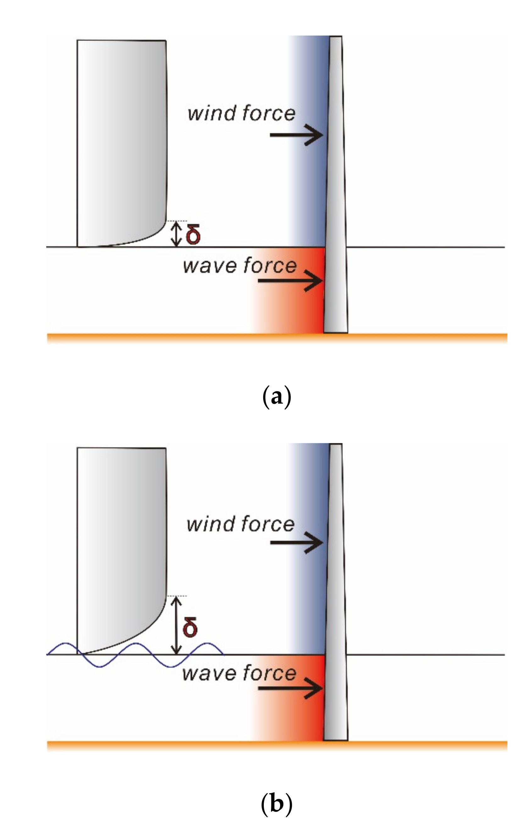
The dynamic load on the substructure of the offshore wind energy converter consists of an aerodynamic force, a hydrodynamic force, and the motion-dependent force that depends on the offshore wind energy converter’s behavior. Once the converter is deflected by aerodynamic force and hydrodynamic force, the flow field near the converter is disturbed, which results in an additional force and a consequent deflection. The aeroelastic instability during this process is called galloping, and the amplitude of structural vibration increases across the direction of the wind.

2.1. Wind Force

In the wake of the offshore wind energy converter’s circular substructure, very complex flows develop due to the sudden expansion of the flow area and its resultant adverse pressure gradient. Once the flow becomes complex, the pressure at the rear side of the offshore wind energy converter cannot fully recover because of the accompanying energy loss and remains significantly lower than that at the front. Due to the presence of these pressure differences, the offshore wind energy converter is exposed to the force that acts in the direction of the flow, and these forces are a form drag that can be written as follows:

$$F_D(t)=\frac{1}{2}{C}_D{\rho }_{air}{A}_S{U}_{air}^2$$

(1)

where $C_D$ is the drag coefficient that depends on the angle of attack, ${\rho }_{air}$ is the density of air, $A_S$ is the projected cross-sectional area, and $U_{air}$ is the wind velocity (see Figure 4).

Moreover, vortices are alternatively swept away from the left and right edges of the offshore wind energy converter’s circular substructure, which eventually leads to Von Karman’s vortex street formation. The instantaneous asymmetric pressure distribution with respect to the flow direction as the forgoing vortices are swept away introduces forces that act across the flow direction. Therefore, the offshore wind energy converter is exposed to regularly redirected lateral forces as well as the aforementioned form drag. The lateral forces can be written as:

$$F_L(t)=\frac{1}{2}{C}_L{\rho }_{air}{B}_S{U}_{air}^2$$

(2)

where $C_L$ is the lift coefficient that depends on the angle of attack, and $B_S$ is the projected cross-sectional area, respectively. The period of the lateral force $T_L$ depends on the Strouhal NO. S, which can be written as:

$$S=\frac{nD}{\overline{U}}$$

(3)

where $n$ is the frequency of the lateral force defined as $1/T_L$, $\overline{U}$ is the average wind velocity, and $D$ is the diameter of the monopile. Here, $T_L$ can be interpreted as the interval between the vortices detached from the monopile. Therefore, the frequency of the lateral drag is defined as $2n$.

When exposed to a periodic lateral force, the offshore wind energy converter can vibrate; in this case, the vibration’s amplitude does not surpass half the diameter of the monopile foundation. However, as the Strouhal period approaches the offshore wind energy converter’s natural period, the vibration is amplified and severely influences the nearby flow field.

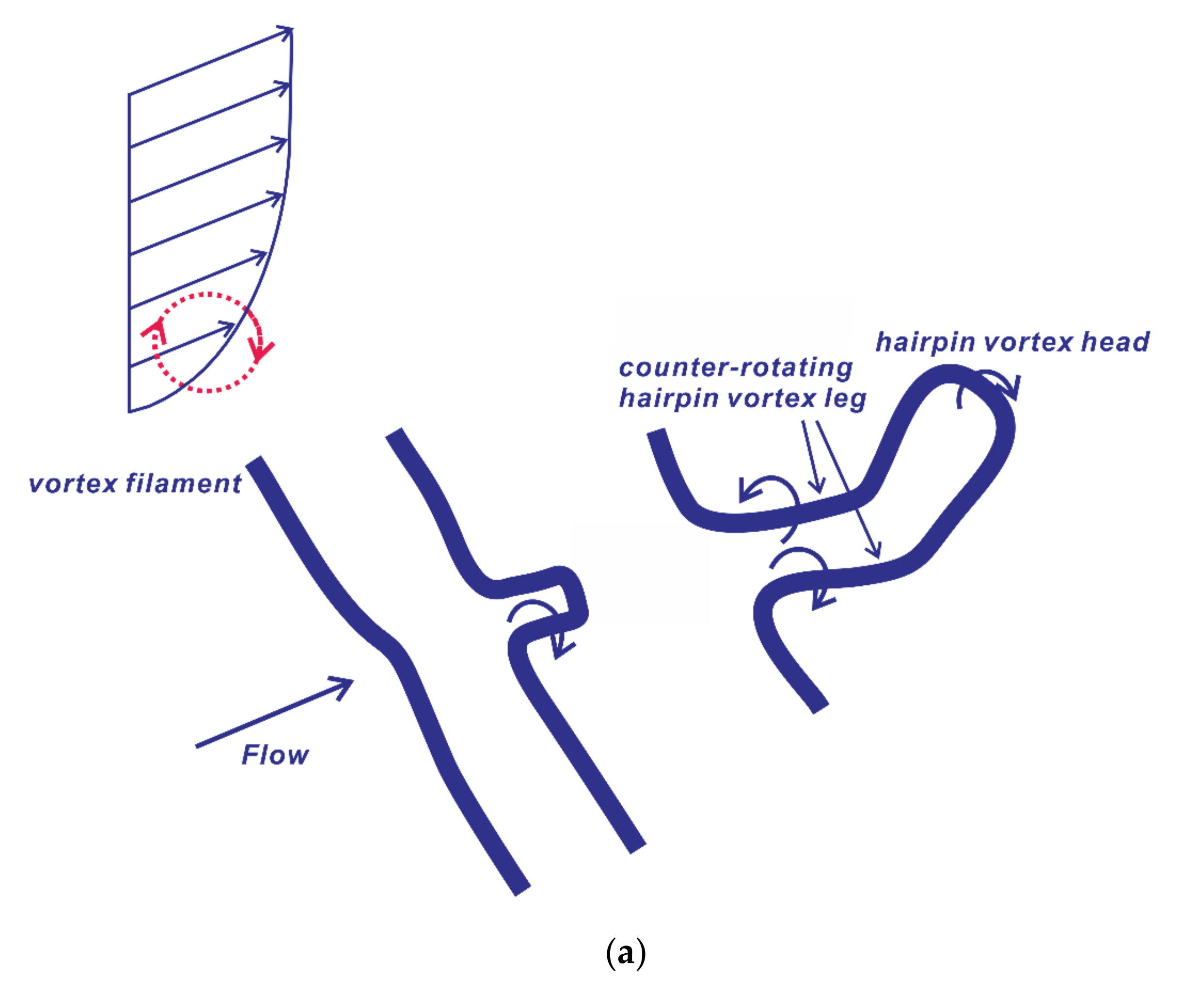
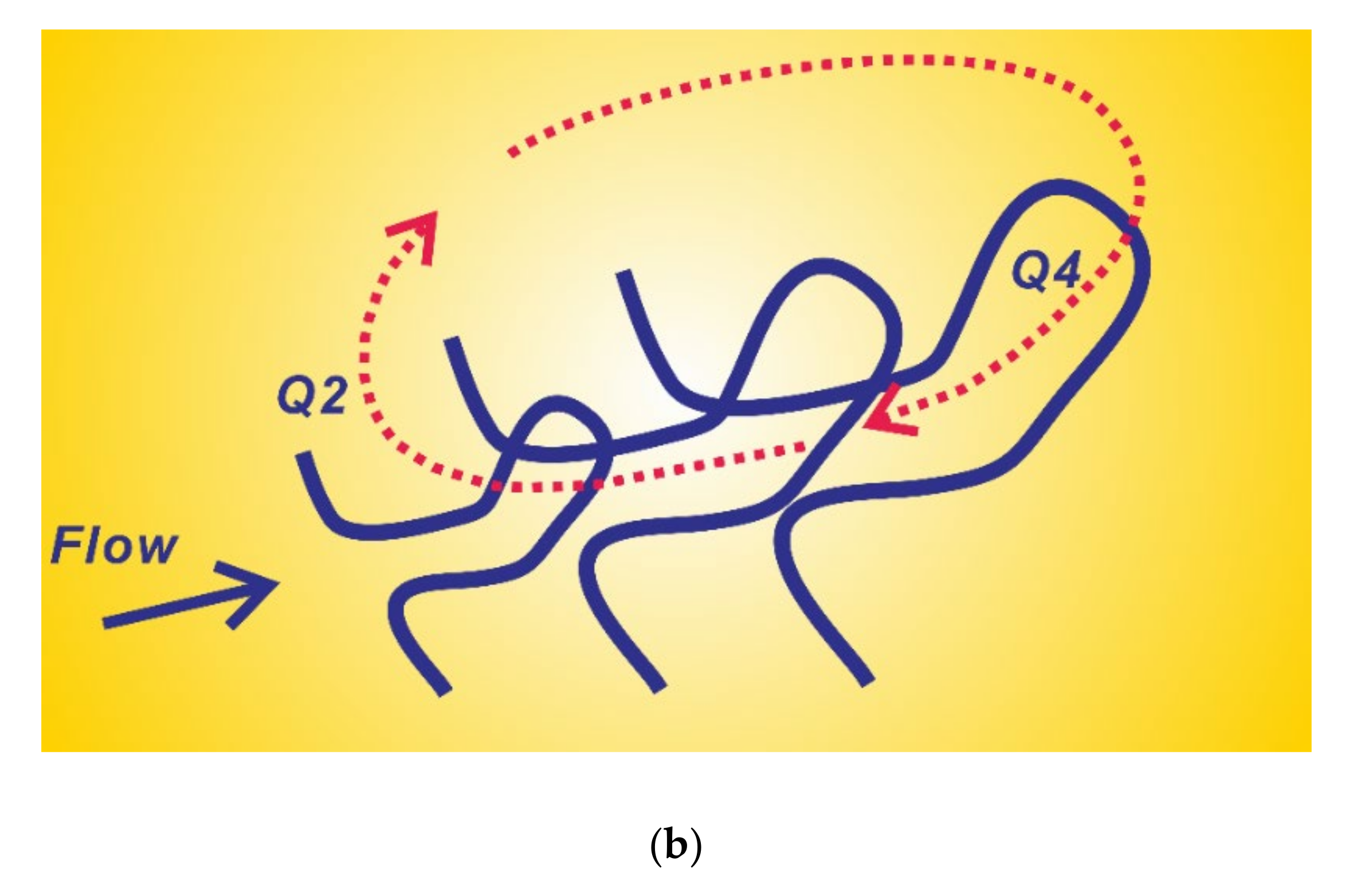
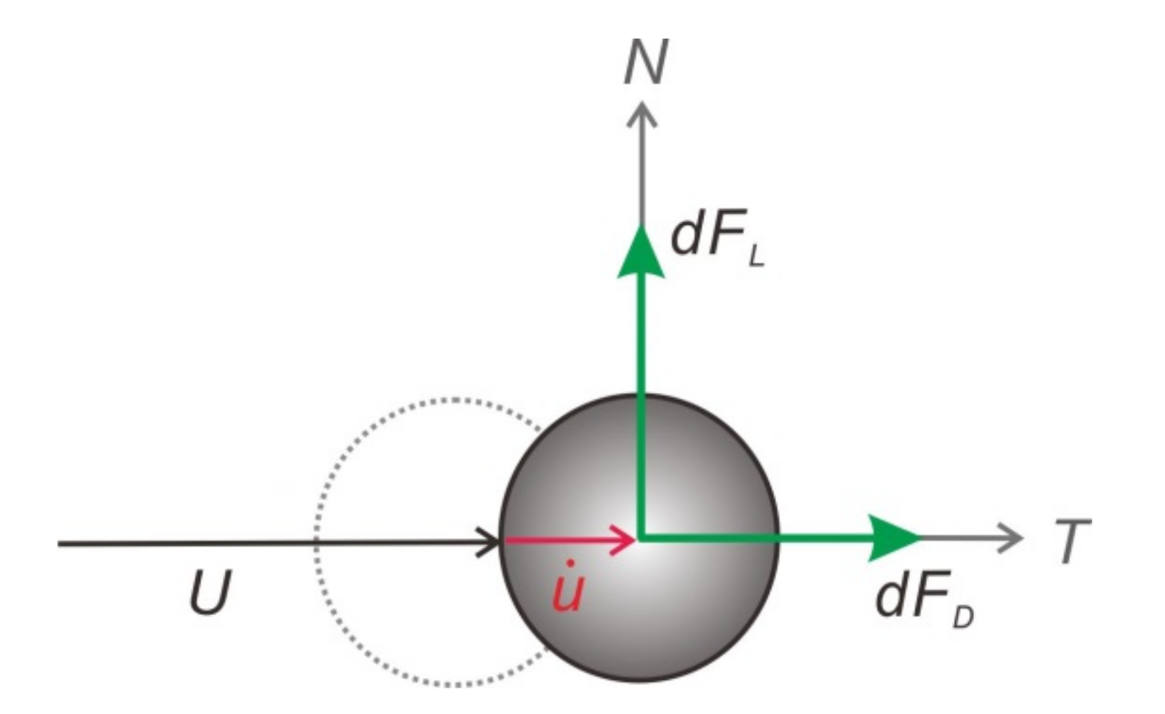
2.2. Aerodynamic Damping

If the offshore wind energy converter is deflected as $u$ due to the aerodynamic force along the direction of wind, the relative wind velocity $U_r$ with respect to the offshore wind energy converter can be defined as (see Figure 5):

$$U_r=U-\dot{u}$$

(4)

and the drag force per unit width can be written as:

$$F_D(t)=\frac{1}{2}{C}_D{\rho }_{air}{A}_S{(U_{air}-\dot{u})}^2$$

(5)

Assuming that $\dot{u}/U_{air}$ is small, the above expression can be approximated as:

$$F_D(t)\cong \frac{1}{2}{C}_D{\rho }_{air}{A}_S{U}_{air}^2\left(1-\frac{2\dot{u}}{U_{air}}\right)$$

(6)

Therefore, the aerodynamic damping $C_D{\rho }_{air}{A}_S{U}_{air}\dot{u}$ is additionally introduced.

2.3. Random Wave Force

The wave force acting on the substructure of the offshore wind energy converter can be classified as a small body and a large body according to the relative scale of the substructure over the wavelength. In the case of a small body, both the disturbance in waves owing to the presence of substructure and the diffraction due to the offshore wind energy converter can be neglected while they should be taken into full consideration in the case of a large body [8]. In the case of the monopile considered in this study, the diameter D is around 5 m, the design wave period T is around 10 s, and the water depth is 20 m. Therefore, this monopile can be classified as a small body since D/L is 0.04 where L is wavelength and has a value of 121 m. Following the Morrison formula [9], the wave force can be written as [5]:

$$p_{wave}\left(x,t\right)=\frac{1}{2}{C}_d\rho A_S{U}_f^2+C_m\rho V{\dot{U}}_f$$

(7)

where $C_d$ is the hydrodynamic drag coefficient, $C_m$ is the inertia force coefficient, $\rho$ is the density of water, $U_f$ and ${\dot{U}}_f$ are the water velocity and acceleration due to waves, respectively, and $V$ is a volume per unit length of the substructure [10].

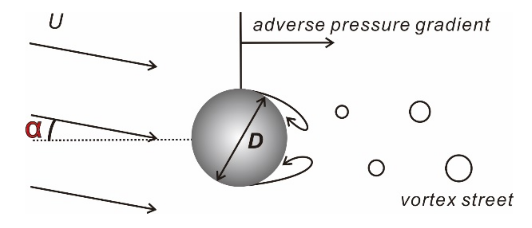
2.4. Hydrodynamic Damping

The offshore wind energy converter’s deflection within the water introduces the relative velocity between the water particle and the offshore wind energy converter. Eventually, hydrodynamic damping via the drag acts on the offshore wind energy converter. If the converter is installed in shallow water, the underwater substructure is generally composed of a highly rigid material. In this case, hydrodynamic damping is negligible since the deflection is relatively small.

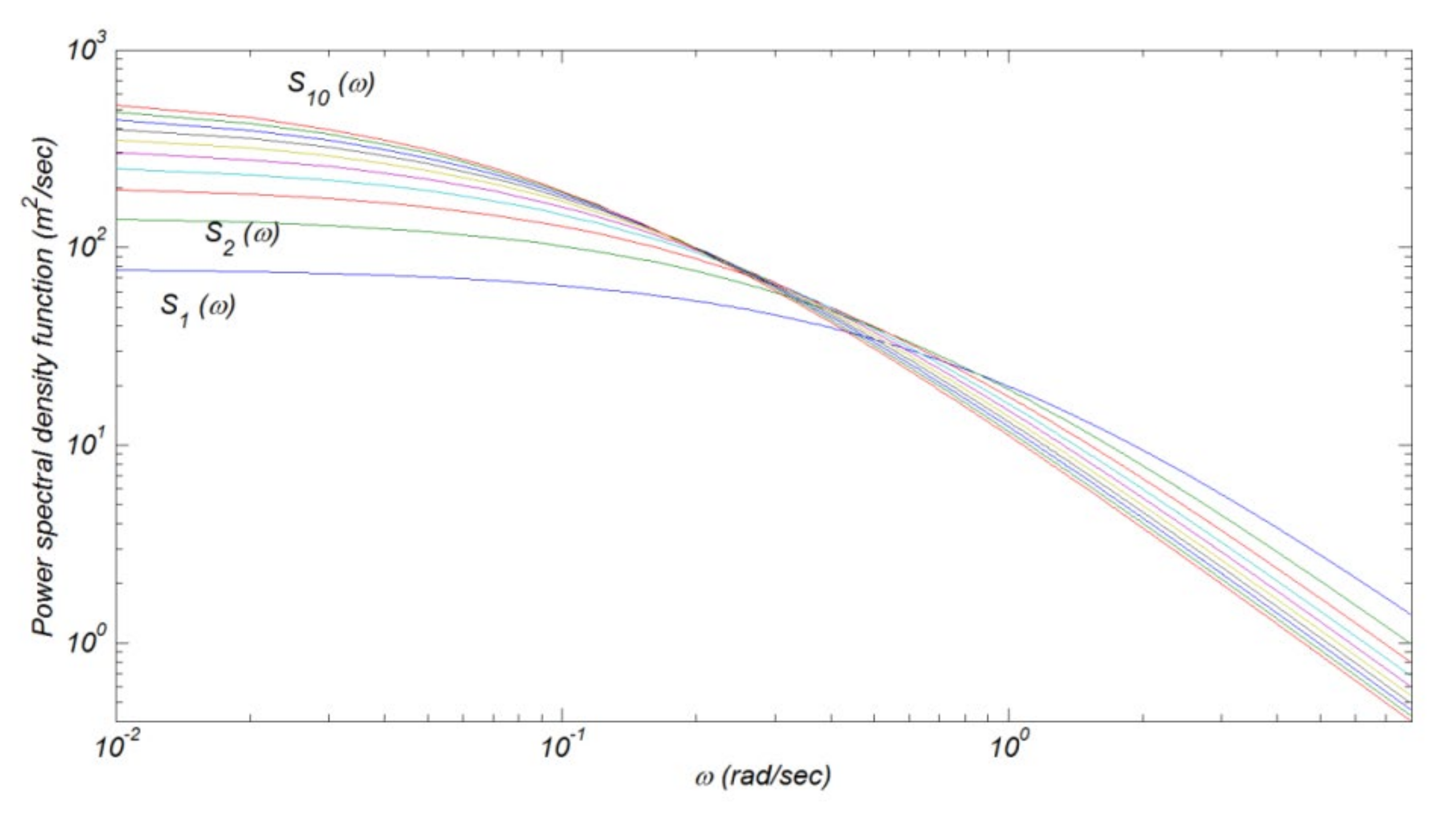
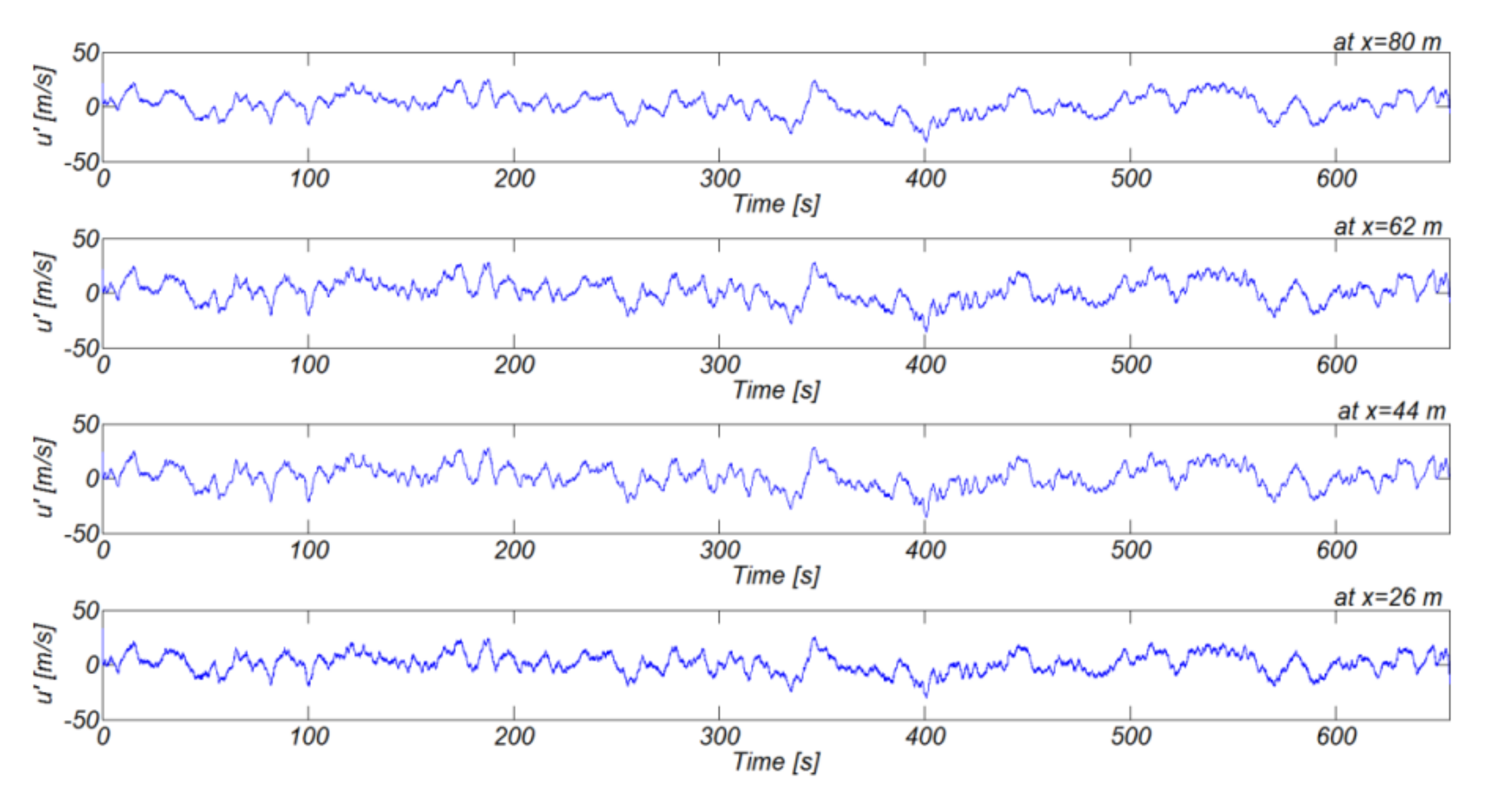
3. Monte Carlo Simulation of the Wind Velocity

3.1. Kaimal Spectrum and Cross-Spectrum

The weather conditions are classified as mild or storm and can be described in terms of the wind speed $U_{10}$ averaged over 10 min, the shear stress, and the turbulence intensity ${\sigma }_U/U_{10}$. Here, the shear stress is defined as the gradient of the vertical profile of longitudinal wind velocity, and the turbulence intensity ${\sigma }_U/U_{10}$ is defined as the standard deviation of the wind velocity around its mean value, based on the assumption that the wind velocity is sustained to be steady-state over a short period of about 10 min. The moderate wind is used to analyze the offshore wind energy converter’s fatigue behavior, and the storm is used as a design load for the offshore wind energy converter [11]. Because the wind over the short temporal and spatial domain of the limited scope is closely correlated, a numerical simulation of the turbulent wind velocity components along the offshore wind energy converter [12] has been implemented using the cross-spectrum. For the sake of self-containment, the numerical simulation procedure of instantaneous turbulent wind velocity using the cross-spectrum can be summarized as:

For brevity, the instantaneous wind speed $U_{air}\left(x,t\right)$ is decomposed into the mean velocity ${\overline{U}}_{air}\left(x\right)$ and the turbulent component $u^{\prime }\left(x,t\right)$, and can be written as (see Figure 6):

$$U_{air}\left(x,t\right)={\overline{U}}_{air}\left(x\right)+u^{\prime }\left(x,t\right)$$

(8)

Here, the mean wind velocity ${\overline{U}}_{air}\left(x\right)$ is known to follow a logarithmic distribution, which can be written as [10]:

$$\frac{{\overline{U}}_{air}\left(x\right)}{{\overline{U}}_{ref}}=\ln \left(\frac{x}{x_o}\right)$$

(9)

where ${\overline{U}}_{ref}$ is the reference wind velocity that is usually taken as the mean velocity at a height of 10 m, and $x_o$ is the roughness height. Under stormy weather conditions in open seas with ${\overline{U}}_{ref}$ at a 10 m height that ranges from 10 to 20 m/s, the roughness height is known to have a value of 1–10 cm [13]. ${\overline{U}}_{ref}$ is irregular due to the variability inherent in the marine environment [14,15,16] and is known to follow a Weibull distribution, which can be written as:

$$F_{{\overline{U}}_{ref}}\left({\overline{U}}_{ref}\right)=1-\exp \left[-{\left(\frac{{\overline{U}}_{ref}}{A_W}\right)}^k\right]$$

(10)

where the scale parameter $A_W$ and the shape parameter $k$ are site and height dependent [11]. On the other hand, the turbulence component $u^{\prime }\left(x,t\right)$ in Equation (8) has been perceived to follow a Gaussian stochastic process of a zero mean, the statistical characteristics of which can described by the cross spectrum between the turbulence components at $x$ and $x^{\prime }$ (see Figure 6). The cross-spectral density function $S_{u^{\prime }}\left(x,x^{\prime }\right)$ can be written as [17]:

$$S_{u^{\prime }}\left(x,x^{\prime }\right)=\sqrt{S_{u^{\prime }}\left(x\right)S_{u^{\prime }}\left(x^{\prime }\right)}Co{h}_{u^{\prime }}\left(x,x^{\prime }\right)$$

(11)

where $S_{u^{\prime }}\left(x\right)$ is a spectral density function of the turbulence velocity component $u^{\prime }\left(x,t\right)$, and $Co{h}_{u^{\prime }}\left(x,x^{\prime }\right)$ is the coherence function.

Following the Kaimal spectrum that has been the most preferred in the literature [18], $S_{u^{\prime }}\left(x\right)$ in Equation (11) can be written as:

$$S_{u^{\prime }}\left(x\right)=\frac{{\sigma }_{u^{\prime }}^2}{n}\frac{4F(x)}{{\left[1+70.8F^2(x)\right]}^{5/6}}$$

(12)

where

$${\sigma }_{u^{\prime }}^2=u_{*}^2\left[6-\frac{1.1}{\tan \left(\ln x_0+1.75\right)}\right]$$

(13)

$$u_{*}={(0.006)}^{1/2}{\overline{U}}_{air}(x=10)$$

(14)

where $n$ is a frequency, $u_{*}$ is a friction velocity, ${\overline{U}}_{air}\left(x=10\right)$ is the mean wind velocity at 10 m height, and $F(x)$ is the nondimensional frequency depending on the vertical position. $F(x)$ can be written as:

$$F(x)=\frac{n{L}_{u^{\prime }}(x)}{{\overline{U}}_{air}(x)}$$

(15)

where $L_{u^{\prime }}(x)$ denotes the characteristic length scale of the turbulence given as:

$$L_{u^{\prime }}(x)=300{\left(\frac{x}{200}\right)}^{\nu }$$

(16)

$$\nu =0.67+0.05\ln (x_o)$$

(17)

The coherence function $Co{h}_{u^{\prime }}\left(x,x^{\prime }\right)$ in Equation (11) can be written as:

$$Co{h}_{u^{\prime }}\left(x,x^{\prime }\right)=\exp \left(-\frac{\left|n\right|\sqrt{C_A{}^2\left|x-x^{\prime }\right|}}{2\pi \left[{\overline{U}}_{air}(x)+{\overline{U}}_{air}(x^{\prime })\right]}\right)$$

(18)

where $C_A$ is an attenuation coefficient that is inversely proportional to the degree of correlation of the turbulence velocity components at x and x’; it usually has a value of 10 [17,19].

3.2. Monte Carlo Simulation

After discretizing the monopile of the offshore wind energy converter with I nodes (see Figure 5), the turbulent velocity components $u_i{}^{\prime }$$\left[i=1,2,\cdots ,I\right]$ at each node can be written as using the cross spectral density function $S_{ij}$$\left[i,j=1,2,\cdots ,I,i\ne j\right]$ in Equation (11) and the self-spectral density function $S_{ii}$$\left[i=1,2,\cdots ,I\right]$ in Equation (12):

$$\left[\begin{array}{c}{u_1}^{\prime }\\ {u_2}^{\prime }\\ {u_3}^{\prime }\\ ·\\ ·\\ ·\\ ·\\ {u_I}^{\prime }\end{array}\right]=\left[\begin{array}{ccccccc}\int S_{11}^{1/2}& \int S_{12}^{1/2}& \int S_{13}^{1/2}& ·& ·& ·& \int S_{1I}^{1/2}\\ \int S_{21}^{1/2}& \int S_{22}^{1/2}& \int S_{23}^{1/2}& ·& ·& ·& \int S_{2I}^{1/2}\\ \int S_{31}^{1/2}& \int S_{32}^{1/2}& \int S_{33}^{1/2}& ·& ·& ·& \int S_{3I}^{1/2}\\ ·& ·& ·& ·& ·& ·& ·\\ ·& ·& ·& ·& ·& ·& ·\\ ·& ·& ·& ·& ·& ·& ·\\ ·& ·& ·& ·& ·& ·& ·\\ \int S_{I1}^{1/2}& \int S_{I2}^{1/2}& \int S_{I3}^{1/2}& ·& ·& ·& \int S_{II}^{1/2}\end{array}\right]\left[\begin{array}{c}{e}^{i\omega t}d\omega \\ e^{i\omega t}d\omega \\ e^{i\omega t}d\omega \\ ·\\ ·\\ ·\\ ·\\ e^{i\omega t}d\omega \end{array}\right]$$

(19)

The matrix in Equation (19) is always positive since it excludes an imaginary part that explains a lagging time for the air wave. Hence, Cholesky’s method can be utilized to decompose $S$ such as the following:

$$S=H(\omega )H^{T*}(\omega )$$

(20)

where the superscript ^T denotes the transpose of the matrix, and the superscript * denotes the complex conjugate. The lower triangular matrix $H(\omega )$ can be written as:

$$H(\omega )=\left[\begin{array}{ccccccc}{H}_{11}& & & & & & \\ H_{21}& H_{22}& & & & & \\ H_{31}& H_{32}& H_{33}& & & & \\ \cdot & \cdot & \cdot & \cdot & & & \\ \cdot & \cdot & \cdot & \cdot & \cdot & & \\ \cdot & \cdot & \cdot & \cdot & \cdot & \cdot & \\ H_{I1}& H_{I2}& H_{I3}& \cdot & \cdot & \cdot & H_{II}\end{array}\right]$$

(21)

and in terms of $H(\omega )$, the turbulent wind velocities $u_1{}^{\prime }(t)$, $u_2{}^{\prime }(t)$, and $u_3{}^{\prime }(t)$ at nodes 1, 2, and 3, respectively, can be written as:

$$u_j{}^{\prime }(t)=2{\displaystyle \sum _{m=1}^3{\displaystyle \sum _{l=1}^N\left|H_{jm}\left({\omega }_{ml}\right)\right|}\sqrt{\Delta \omega }\cos \left[{\omega }_{ml}t-{\theta }_{jm}\left({\omega }_{ml}\right)+{\mathsf{\Phi }}_{ml}\right]}$$

(22)

For the sake of clarity, we explicitly rewrite the above equation for I = 3 as:

$$u_1{}^{\prime }(t)=2{\displaystyle \sum _{l=1}^N\left|H_{11}\left({\omega }_{1l}\right)\right|\sqrt{\Delta \omega }}\cos \left[{\omega }_{1l}t-{\theta }_{11}\left({\omega }_{1l}\right)+{\mathsf{\Phi }}_{1l}\right]$$

(23)

$$u_2{}^{\prime }(t)=2\left({\displaystyle \sum _{l=1}^N\left|H_{21}\left({\omega }_{1l}\right)\right|\sqrt{\Delta \omega }}\cos \left[{\omega }_{1l}t-{\theta }_{21}\left({\omega }_{1l}\right)+{\mathsf{\Phi }}_{1l}\right]+{\displaystyle \sum _{l=1}^N\left|H_{22}\left({\omega }_{2l}\right)\right|\sqrt{\Delta \omega }}\cos \left[{\omega }_{2l}t-{\theta }_{22}\left({\omega }_{2l}\right)+{\mathsf{\Phi }}_{2l}\right]\right.\left.+{\displaystyle \sum _{l=1}^N\left|H_{23}\left({\omega }_{2l}\right)\right|\sqrt{\Delta \omega }}\cos \left[{\omega }_{3l}t-{\theta }_{23}\left({\omega }_{3l}\right)+{\mathsf{\Phi }}_{3l}\right]\right)$$

(24)

$$u_3{}^{\prime }(t)=2\left({\displaystyle \sum _{l=1}^N\left|H_{31}\left({\omega }_{1l}\right)\right|\sqrt{\Delta \omega }}\cos \left[{\omega }_{1l}t-{\theta }_{31}\left({\omega }_{1l}\right)+{\mathsf{\Phi }}_{1l}\right]\right.+{\displaystyle \sum _{l=1}^N\left|H_{32}\left({\omega }_{2l}\right)\right|\sqrt{\Delta \omega }}\cos \left[{\omega }_{2l}t-{\theta }_{32}\left({\omega }_{2l}\right)+{\mathsf{\Phi }}_{2l}\right]\left.+{\displaystyle \sum _{l=1}^N\left|H_{33}\left({\omega }_{3l}\right)\right|\sqrt{\Delta \omega }}\cos \left[{\omega }_{3l}t-{\theta }_{33}\left({\omega }_{3l}\right)+{\mathsf{\Phi }}_{3l}\right]\right)$$

(25)

where ${\mathsf{\Phi }}_{ij}$ is a random phase uniformly distributed over the interval $[0,2\pi ]$, and the angular frequency ${\omega }_{ml}$ [radian/s] with two subscripts is a measure to secure the stationary stochastic process of the turbulent wind velocity and can be written as [20]:

$${\omega }_{1l}=l\Delta \omega -\frac{2}{3}\Delta \omega ,l=1,2,\cdots ,N$$

(26)

$${\omega }_{2l}=l\Delta \omega -\frac{1}{3}\Delta \omega ,l=1,2,\cdots ,N$$

(27)

$${\omega }_{3l}=l\Delta \omega ,\hspace{1em}l=1,2,\cdots ,N$$

(28)

$${\theta }_{jm}\left({\omega }_{ml}\right)={\tan }^{-1}\frac{\mathrm{Im}\left[H_{jm}\left({\omega }_{ml}\right)\right]}{\mathrm{Re}\left[H_{jm}\left({\omega }_{ml}\right)\right]}$$

(29)

where $N$ is the total number of harmonic components used in the numerical simulation, and ${\omega }_u$ is the cut-off frequency.

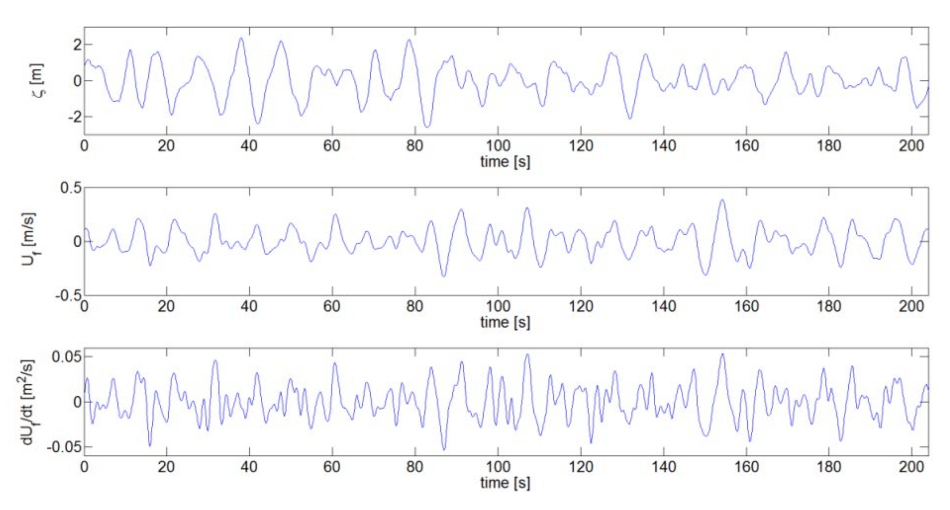
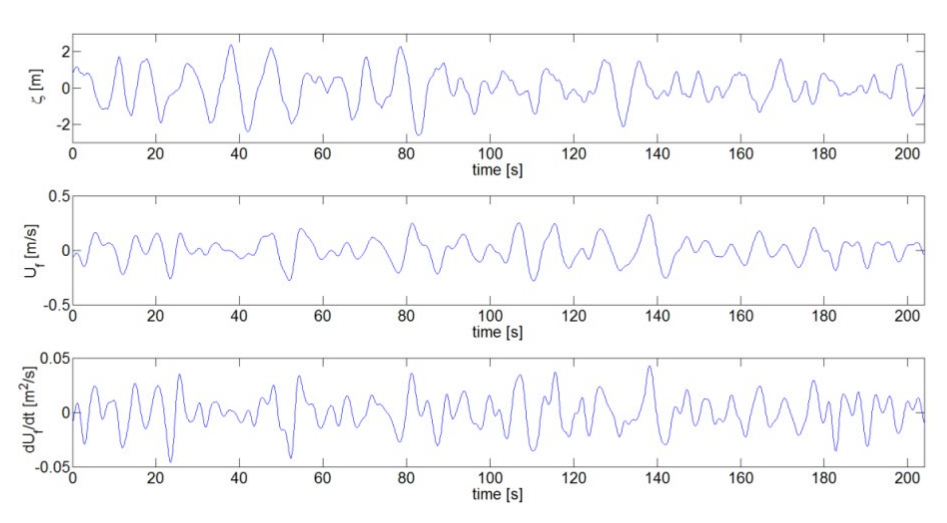
4. Numerical Simulation of Random Waves Using the Random Phase Method

The sample time series of the random waves and its induced velocity and acceleration are numerically simulated using the Random Phase Method based on the JONSWAP (Joint North Sea Wave Project) wave spectrum, its associated velocity spectrum, and acceleration spectrum. The JONSWAP spectral density function $S_{\zeta \zeta }(f)$, the velocity spectral density function $S_{U_f{U}_f}(f)$, and the acceleration spectral density function $S_{{\dot{U}}_f{\dot{U}}_f}(f)$ are given as [21]:

$$S_{\zeta \zeta }(f)=\frac{{\alpha }_p{g}^2}{f^5}\exp \left(-\frac{5}{4}\frac{f_p^4}{f^4}\right){\gamma }^{\exp \left[-\frac{{\left(f-f_p\right)}^2}{2{\sigma }^2{f}_p^2}\right]}$$

(30)

$$S_{U_f{U}_f}(f)={\omega }^2{S}_{\zeta \zeta }(\omega )\frac{{\cosh }^{2}k\left(z+h\right)}{{\sinh }^{2}kh}$$

(31)

$$S_{{\dot{U}}_f{\dot{U}}_f}(f)={\omega }^4{S}_{\zeta \zeta }(\omega )\frac{{\cosh }^{2}k\left(z+h\right)}{{\sinh }^{2}kh}$$

(32)

where $f$ is a frequency [Hz], $f_p$ is the peak frequency, $\gamma$ is the peak enhancement factor, and ${\alpha }_p$ is the frequency spectrum bandwidth factor [Phillips coefficient] given as:

$${\alpha }_p=5\left(\frac{H_s^2{f}_p^4}{g^2}\right)\left(1-0.287\ln \gamma \right){\pi }^4$$

(33)

$$\sigma =\left\{\begin{array}{ccc}0.07& IFF& f<f_p\\ 0.09& IFF& f>f_p\end{array}\right.$$

(34)

$$\gamma =\left\{\begin{array}{ccc}5& for& \frac{T_p}{\sqrt{H_s}}\le 3.6\\ e^{5.75-1.15\times \frac{T_p}{\sqrt{H_s}}}& for& 3.6\le \frac{T_p}{\sqrt{H_s}}\le 5\\ 1& for& 5\le \frac{T_p}{\sqrt{H_s}}\end{array}\right.$$

(35)

Here $\gamma$ is in the range from 1 to 6 for ocean waves, while ${\alpha }_p$ is in the range of 0.0081 to 0.1. The values $\gamma =1$ and ${\alpha }_p=0.081$ provide a spectrum of fully developed wind waves. We used $\gamma =3$, ${\alpha }_p=0.025$, and $\sigma =0.08$, which correspond to the underdeveloped wind waves as can be found on the west coast of the Korean Peninsula due to the limited fetch length [22].

In the process of simulating the design waves at the site of the structure, the wave height and the period are determined using a zero up-crossing method. The mean period $T_Z$ of the event where the water surface crosses the mean water level with a positive slope and the peak period $T_P$ satisfy the following relationship:

$$T_Z=T_P\sqrt{\frac{5+\gamma }{11+\gamma }}$$

(36)

In the case of fully developed waves with $\gamma =1$, the above relationship is reduced to:

$$T_P=1.414T_Z$$

(37)

We numerically generated random waves using the random phase method. In the random phase method, wave trains are generated by combining the discrete wave energy spectrum that corresponds to the target spectrum with a random phase synthesized from a random number generator. This yields the Fourier transform of the time series with the target wave energy spectrum. The corresponding time series can be obtained through an inverse Fourier transformation.

The steps to simulate the time series using a random phase method can be summarized as follows [21,23]:

• Define a target wave energy spectrum.
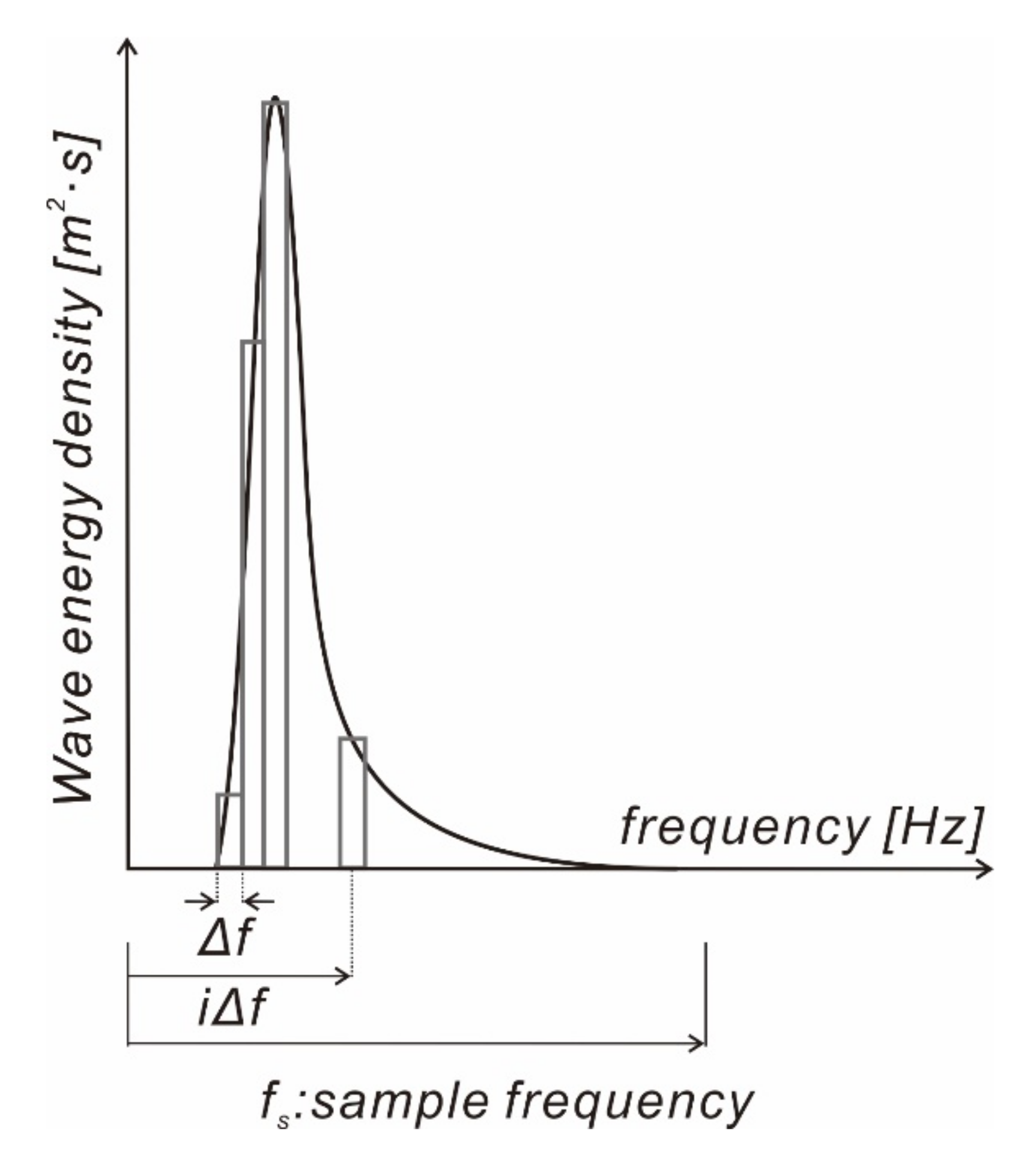
• Choose the sample frequency $f_s$ and the resolution of the spectrum (half the number of Fourier components) $N$. This yields a frequency domain resolution of $\Delta f=f_s/N$. The discrete wave energy spectrum ${\sigma }_{\varsigma }\left(f_i\right)$ can be written as (see Figure 7):

  $${\sigma }_{\varsigma }^2\left(f_i\right)=S_{\varsigma }\left(i\Delta f\right)\times \Delta f,f_i=i\Delta f,i=1,2,\dots ,N$$

  (38)
• Calculate the N complex Fourier coefficients $C\left(f_i\right)=A\left(f_i\right)+iB\left(f_i\right)$ by picking a random phase $\psi (f_i)$ between 0 and 2π for all frequencies smaller than the Nyquist frequency $f_N=f_s/2$. A and B are given by:

  $$A\left(f_i\right)=\sqrt{\frac{{\sigma }_x^2\left(f_i\right)}{2}}\cos \left(\psi \left(f_i\right)\right)$$

  (39)

  $$B\left(f_i\right)=\sqrt{\frac{{\sigma }_x^2\left(f_i\right)}{2}}\sin \left(\psi \left(f_i\right)\right)$$

  (40)
• Mirror the N Fourier components into the Nyquist frequency $f_N$ in order to obtain a Hermitian Fourier transform

  $$C_{N+i}=C_{N-i+1}^{\ast },i=1,2,\cdots ,N$$

  (41)

  where the superscript * denotes a complex conjugate.
• Apply the inverse Fourier transform to $C\left(f_i\right)$ and calculate the time series of the water surface displacement $\varsigma \left(t\right)$ as follows

  $$\varsigma \left(t\right)={\displaystyle \int C\left(f\right)e^{-i2\pi ft}df}$$

  (42)

5. Equations of Motion for the Offshore Wind Energy Converter

If the structure is slender like the monopile as a substructure of the offshore wind energy converter, among many structural member forces, the bending moment dominates. Following D’Alembert, the inertial force resulting from the deflection $z$ could be regarded as a kind of external force (see Figure 8). This external force is then balanced by the resistance bending moment that develops in the structural member. From the principle of virtual work (see Figure 9), we can obtain the following equation of motion [24]:

$$\tilde{m}\ddot{z}+\tilde{k}z=\widetilde{p(t)}$$

(43)

where

$$\tilde{m}={\displaystyle {\int }_0^{L}m{\mathsf{\Psi }}^2(x)dx}$$

(44)

$$\tilde{k}={\displaystyle {\int }_0^{L}EI{\mathsf{\Psi }}^2(x)dx}$$

(45)

$$\widetilde{p(t)}={\displaystyle {\int }_0^L{f}_E(x,t)\mathsf{\Psi }(x)dx}$$

(46)

In Equations (43)–(46), $\tilde{m}$ is the mass, $EI$ is the moment stiffness, $\mathsf{\Psi }(x)$ is the shape function, and $f_E(x,t)$ is the environmental load.

$f_E(x,t)$ consists of wind and a random wave force and can be written as:

$$f_E(x,t)=p_{wind}(x,t)+p_{wave}(x,t)$$

(47)

According to the Morrison formula, the wind and random wave forces can be written as:

$$p_{wind}(x,t)=\overline{p_{wind}}(x)+{p^{\prime }}_{wind}(x,t)$$

(48)

$$\overline{p_{wind}}(x)=\frac{1}{2}{C}_D{\rho }_{air}A{\overline{U}}_{air}{}^2$$

(49)

$${p^{\prime }}_{wind}(x,t)=\frac{1}{2}{C}_D{\rho }_{air}A\overline{U_{air}}{U}^{\prime }$$

(50)

$$p_{wave}(x,t)=\frac{1}{2}{C}_d\rho A{U}_f^2+C_m\rho V{\dot{U}}_f$$

(51)

In Equations (48)–(50), $\overline{\cdot }$ denotes the time average, which will be omitted hereafter for the sake of brevity.

In order for the aerodynamic and hydrodynamic damping to be unveiled, we first rewrite the drag terms of the random waves and the wind force in terms of the relative velocity $U_{air}-\dot{u}$. We can then obtain the following relationships.

$$p_{wind}={\displaystyle {\int }_h^L\frac{1}{2}{C}_D{\rho }_{air}A{\left(U_{air}-\dot{u}\right)}^2\mathsf{\Psi }dx}\cong {\displaystyle {\int }_h^L\frac{1}{2}{C}_D{\rho }_{air}A{U}_{{}^{air}}^2\mathsf{\Psi }dx-\dot{z}{\displaystyle {\int }_h^L{C}_D{\rho }_{air}A{U}_{air}{\mathsf{\Psi }}^{2}dx}}$$

(52)

$${p^{\prime }}_{wind}={\displaystyle {\int }_h^L\frac{1}{2}{C}_D{\rho }_{air}A\left(U_{air}-\dot{u}\right)U^{\prime }\mathsf{\Psi }dx}={\displaystyle {\int }_h^L\frac{1}{2}{C}_D{\rho }_{air}A{U}_{air}{U}^{\prime }\mathsf{\Psi }dx}-\dot{z}{\displaystyle {\int }_h^L\frac{1}{2}{C}_D{\rho }_{air}A{U}^{\prime }{\mathsf{\Psi }}^{2}dx}$$

(53)

$$p_{wave\_D}={\displaystyle {\int }_0^h\frac{1}{2}{C}_d\rho A{\left(U_f-\dot{u}\right)}^2\mathsf{\Psi }(x)dx}\cong {\displaystyle {\int }_0^h\frac{1}{2}{C}_d\rho A{U}_f^2\mathsf{\Psi }(x)dx}-\dot{z}{\displaystyle {\int }_0^h{C}_d\rho A{U}_f{\mathsf{\Psi }}^2(x)dx}$$

(54)

$$p_{wave\_i}={\displaystyle {\int }_0^h{C}_m\rho V{\left({\dot{U}}_f-\ddot{u}\right)}^2\mathsf{\Psi }dx}\cong {\displaystyle {\int }_0^h{C}_m\rho V{\dot{U}}_f\mathsf{\Psi }dx}-\ddot{Z}{\displaystyle {\int }_0^h{C}_m\rho V{\mathsf{\Psi }}^{2}dx}$$

(55)

In order for the physical meaning of the aerodynamic damping to become more visible, the damping term is moved to the left-hand side of the equation, and after some elaboration, the equation of motion can be rewritten as:

$$M\ddot{z}+C\dot{z}+Kz=P$$

(56)

where the mass $M$, the damping coefficient $C$, the spring coefficient $K$, and the external force $P$ are given as:

$$M={\displaystyle {\int }_0^{L}m{\psi }^2(x)dx+}{\displaystyle {\int }_0^L{C}_m\rho V{\psi }^{2}dx}$$

(57)

$$C={\displaystyle {\int }_0^{L}c{\psi }^{2}dx+}{\displaystyle {\int }_h^L{C}_D{\rho }_{air}A\left[U_{air}+\frac{1}{2}{U}^{\prime }\right]{\psi }^{2}dx}+{\displaystyle {\int }_0^h{C}_d\rho A{U}_f{\psi }^{2}dx}$$

(58)

$$K={\displaystyle {\int }_0^{L}EI{\mathsf{\Psi }}^2(x)dx}$$

(59)

$$\begin{gathered} P={\displaystyle {\int }_0^L\frac{1}{2}{C}_D{\rho }_{air}A{U}_{{}^{air}}^2\mathsf{\Psi }dx}+{\displaystyle {\int }_0^L\frac{1}{2}{C}_D{\rho }_{air}A{U}_{air}{U}^{\prime }\mathsf{\Psi }dx}+{\displaystyle {\int }_0^h\frac{1}{2}{C}_d\rho A{U}_f\left|U_f\right|\mathsf{\Psi }(x)dx} \\ +{\displaystyle {\int }_0^h{C}_m\rho V{\dot{U}}_f\mathsf{\Psi }(x)dx}+{\displaystyle {\int }_0^h\frac{1}{2}{C}_d\rho A{U}_f\left|U_f\right|\mathsf{\Psi }(x)dx}+{\displaystyle {\int }_0^h{C}_m\rho V{\dot{U}}_f\mathsf{\Psi }(x)dx} \end{gathered}$$

(60)

In Equation (58), the second term is the damping due to the mean wind velocity, the third term is the damping due to a gust, and the fourth term is the hydrodynamic damping.

In order to describe the motion in terms of the natural frequency ${\omega }_n$, after dividing Equation (56) by $M$ and some additional manipulation, we can rewrite the equation of motion as:

$$\ddot{z}+2\zeta {\omega }_{n}z+{\omega }_n^{2}z=\frac{P}{M}$$

(61)

where $\zeta$ is the damping coefficient, and ${\omega }_n$ is the natural frequency. $\zeta$ and ${\omega }_n$ are given as:

$$\zeta =\frac{C}{2M{\omega }_n}$$

(62)

$${\omega }_n^2=\frac{K}{M}$$

(63)

6. Numerical Simulation

6.1. Numerical Results

We numerically simulated the structural behavior of a 5 MW offshore wind energy converter subject to wind and random waves to quantitatively evaluate the nonlinear destructive interaction between wind and wave loads. In order to provide a more accurate analysis, the numerical simulation included an analysis of the buffeting of the converter due to gusts, which has been generally overlooked in the design practice for the offshore wind energy converters in South Korea. A monopile foundation was selected as the substructure for the converter because it is the easiest to deploy. The aero-elastic and hydro-elastic analyses that explain the interaction of the wind and wave forces with the offshore wind energy converter were implemented using the beam element method with a shape function of the first eigenmode in an effort to increase the accuracy of the numerical simulation (see Figure 10).

In doing so, a time series for the wind velocity at 10 different elevations [x = 26, 32, 38,…, 80 m] with a gust effect is therefore required during the buffeting analysis of the offshore wind energy converter. These were numerically simulated using a Monte Carlo technique with a cross spectrum based on the Kaimal spectrum. The weather conditions along the west coast of the Korean Peninsula where a pilot project for an offshore wind energy farm is planned were considered. At that site, the mean wind velocity and friction velocity are taken as ${\overline{U}}_{air}\left(x=10\right)=10.13\mathrm{m}/\mathrm{s}$ and $u_{*}=1.76\mathrm{m}/\mathrm{s}$, respectively. When stormy weather occurs, the roughness height $x_o$ is increased to 0.1 m in order to reflect the bumpy water surface and the ensuing large eddy due to the presence of waves. If the weather is calm, the roughness height $x_o$ is maintained to be at 1.266 mm [2]. The parameters used for numerical simulation are listed in

Table 1. A list of the model parameters used for the numerical simulation.

${\overline{U}}_{air}(x=10)[\mathsf{m}/\mathsf{s}]$	$E_{steel}[\mathsf{P}\mathsf{a}]$	${\rho }_{steel}[{\mathsf{kg}/\mathsf{m}}^3]$	${\rho }_{water}[{\mathsf{kg}/\mathsf{m}}^3]$	$C_d$	$C_m$	$C_D$
10.1314	2.059E + 11	7.980E + 3	1.024E + 3	1.05	1.0	0.5

.

Figure 11 shows the Kaimal spectra at different heights that are used in the numerical simulation. At a higher altitude, a low frequency gust prevails. On the other hand, at a lower altitude, a high frequency gust is dominant.

The maximum wind velocity due to gusts is short-lived, whereas wind waves usually last for three hours. As a result, an average wind speed is considered to be sustained over ten minutes for the design of the converter. When the wave load is considered, it is common for random waves to be simulated for three hours. Figure 12 and Figure 13 depict a numerically simulated sample time series of the turbulent wind velocity using a cross spectrum based on a Kaimal spectrum. Because the scale of the monopile (80 m) is much smaller than the thickness of the atmospheric boundary layer, which easily reaches several hundred meters, it seems that numerically simulated turbulent wind velocities along the monopile are highly correlated with each other. However, at a low height of 26 m, high-frequency components can also be observed. This phenomenon is partially due to the deployment of a coherence function that shows a poor correlation over the high frequency band. However, this trend can also be found in in situ data [3,16].

Figure 14 and Figure 15 depict a numerically simulated time series of the random water waves, its associated velocity, and acceleration at x = 19.0 m, x = 17.5 m. As expected, the water velocity and the acceleration both decrease as descending from the water surface. These observations are consistent with the small-amplitude wave theory. Furthermore, when a comparison is made with numerically simulated turbulent wind velocity, the velocity and the acceleration vary more smoothly. These trends result from the significantly smaller bandwidth for the velocity and acceleration spectrum than that of the Kaimal spectrum. As the size of the bandwidth increases, the irregularity also increases.

Table 2. Summary of wind and wave conditions used in the numerical simulation.

	Wind	Waves
RUN 1	Random Wind [U10 = 10.13 m/s]	Random Waves [Hs = 5 m, Tp = 10 s]
RUN 2	Random Wind [U10 = 10.13 m/s]	NO WAVES
RUN 3	Random Wind [U10 = 10.13 m/s]	Regular Waves [H = 5 m, T = 10 s]
RUN 4	Random Wind [U10 = 10.13 m/s]	Regular Waves [H = 10 m, T = 10 s]
RUN 5	Random Wind [U10 = 10.13 m/s]	Regular Waves [H = 5 m, T = 5 s]

summarizes the wave and wind conditions used for the numerical simulation. Figure 16 depicts the numerically simulated responses of the substructure of the offshore wind energy converter against various combinations of environmental loads. First, the numerical simulation was implemented for the case where the wind and wave load act simultaneously. The numerical simulation was then carried out for the case where only random wind is present. The upper panel corresponds to the case where the random wind and random wave loads act simultaneously, and the lower panel corresponds to the case where only random wind blows. When only random wind blows, the substructure’s response significantly increases. Figure 17 depicts the snapshots of the substructure of the converter when the deflection reaches its maxima. When the deflection reaches its maxima, the maximum displacement for the converter’s substructure is observed as [0.0845 m, −0.0401 m] for RUN1 and [0.1616 m, 0.0359 m] for RUN2.

In Figure 18, we plot the trajectories left behind by the substructure of the offshore wind energy converter in the phase space made with the velocity and the deformation. Here, it is shown that the amplitude of the trajectory significantly decreases along with the stabilizing effect of the waves when compared to the case where only random wind blows. Furthermore, the attractor was shown to move toward the direction of the wind, and these trends are more apparent for the case where only random wind blows. These phenomena are partially caused by the assumption that the mean wind velocity remains unchanged during the numerical simulation, but the deflection can be deduced to be significantly controlled by wavy motions at the water surface occurring as the wind blows. These waves’ stabilizing effects result from the bumpy water surface due to the presence of waves as the wind blows, which then generates a series of hairpin vortices. Later, each hairpin vortex’s solenoidal effects result in the formation of a large eddy circulating in the direction opposite to the incoming wind near the atmospheric boundary layer [1]. As a result, the vertical distribution of the longitudinal wind velocity is modified, and the accompanying energy loss drastically weakens the wind velocity, resulting in less deflection of the converter. In addition to the large eddy mentioned above, a reversal in the wave force’s direction in the third and fourth quadrants also contributes to the waves’ stabilizing effects.

In order to determine the attenuation ratio, the response spectra of the substructure of the offshore wind energy converter are evaluated for various combinations of environmental loads from numerically simulated time series, the results of which are shown in Figure 19. For any combination of external forces, the response spectrum reaches its peak at the natural frequency of the converter (0.78 Hz). For the case where random waves and random wind simultaneously approach the offshore wind energy converter, the response spectrum is reduced over the entire frequency range due to the stabilizing effects of the waves mentioned above, and the response at a natural frequency of 0.78 Hz is reduced by about 30%. For the case with monochromatic waves and random wind, the response spectrum at a natural frequency of 0.78 Hz is significantly reduced. In contrast, the response spectrum increases at a frequency of incoming waves of 10 s. According to variations in the wave period, the changes in the characteristics of the response spectrum were shown to be negligible (Figure 19b). Additionally, as the wave amplitude increases, the response spectrum changes at the natural frequency are invisible, but the response spectrum at the wave period increases as expected (Figure 19b).

6.2. Restriction on the Deflection of the Converter Caused by the Bumpy Water Surface and the Ensuing Large Eddy

In order to analyze the restriction on the deflection of the converter caused by the bumpy water surface and the following large eddy, the trajectory left behind by the drag and inertia forces, which constitute the wave force, are plotted in Figure 20, and the trajectory left behind by the wave and wind forces is depicted in Figure 21. Figure 20 and Figure 21 show that the main external force on the converter’s substructure is a wind with gusts. A pilot project for an offshore wind farm converter will be built on the west coast of the Korean Peninsula, and water depths at that location range from 10 to 20 m, so only 25% of the substructure for the offshore wind energy converter is exposed to incoming waves. Therefore, it is acceptable for wind with gusts to be the main external force on an offshore wind farm on the west coast. For clarity, the vertical distributions of the numerically simulated longitudinal gusts at t = 20 s, t = 137.77 s, t = 279.09 s, t = 479.09 s, and t = 579.09 s are plotted in Figure 22, and the vertical distributions of the mean wind velocity under calm and stormy weather conditions are plotted in Figure 23. Figure 22 and Figure 23 clearly show that under stormy weather conditions, the mean wind velocity is drastically weakened by the bumpy water surface due to waves and the accompanying energy loss. Moreover, the gust direction does not always correspond to the direction of the mean wind field, and during a significant portion of the total simulation period [640 s], the gust moves along the direction opposite to the mean wind field. As a result, the gust was frequently observed to surpass the mean wind velocity easily. Therefore, all of the results observed in this study indicate that the primary external force on the substructure of the offshore wind energy converter is a wind with gusts, and the random waves restrict the deformation of the substructure of the offshore wind energy converter. The randomly fluctuating water surface as the wind blows causes the atmospheric boundary layer to grow nonuniformly, leading to the development of a series of hairpin vortices. Later, each hairpin vortex’s solenoidal effect induces a large eddy swirling in the direction opposite to the incoming wind near the atmospheric boundary layer [5]. As a result, the vertical distribution of the longitudinal wind velocity is modified, the accompanying energy loss drastically weakens the wind velocity, and the deformation of the substructure of the offshore wind energy converter is decreased by 50% when compared with that in the case of wind with gusts over calm seas (Figure 24 and Figure 25). In addition to a large eddy, a reversal in the wave force’s direction in the third and fourth quadrants also contributes to the waves’ stabilizing effects mentioned above.

7. Conclusions

Despite its unlimited growth potential, the offshore wind industry is still suffering from problems, such as the large initial capital requirements. Even though one-third to one-half of the total costs come from installing the offshore wind energy converter, an excessively conservative design for the substructure of the converter exacerbates the problem due to a poor understanding of the nonlinear destructive interaction between wind and wave loads. Even though waves approach an offshore wind energy converter collinearly with the wind, waves and wind forces do not always cause the converter’s substructure to be deformed, and the environmental load can even intermittently exert a force of resistance against deformation. Hence, the excessive initial capital expenditures problem can be quickly addressed by accounting for the nonlinear destructive interaction between wind and wave loads, such as the stabilizing effects of the bumpy water surface on the deflection of the substructure at the design stage. Once these nonlinear destructive interactions are fully realized, the redundant rigidity in the offshore wind energy converter’s substructure can be removed, and extra ductility can be secured, leading to cost savings and improved durability against fatigue fractures. The nonlinear destructive interaction between wind and wave loads acting on the offshore wind energy converter consists of three different mechanisms that can be summarized as follows.

First, an atmospheric boundary layer near the water surface grows nonuniformly when the water surface randomly fluctuates as the wind blows, which then generates a series of hairpin vortices. Later, the solenoidal effects of each hairpin vortex are added, leading to the formation of a large eddy swirling in the direction opposite to the incoming wind near the atmospheric boundary layer [5]. As a result, the vertical distribution of the longitudinal wind velocity is modified, and the wind load on the offshore wind energy converter decreases. Second, the direction of the wave force in the 3rd and 4th quadrants, where the water surface turns into a trough, is eventually reversed and stands in the direction opposite to the wind, so the deflection of the offshore wind energy converter is restricted. Third, aerodynamic damping occurs whenever the offshore wind energy converter is deflected. These deflections cause the relative velocity of wind with respect to the offshore wind energy converter to undergo some changes, eventually introducing aerodynamic damping through a form of drag into the structural system.

In this study, we numerically simulated the structural behavior of a 5 MW offshore wind energy converter subject to various combinations of environmental loads in order to quantitatively evaluate the nonlinear destructive interaction between wind and wave load, which is a crucial step towards the optimal design of the converter achieved by removing the redundant rigidity from the support structure. In order to reflect the bumpy water surface and the subsequent large eddy, the roughness height $x_o$ is increased to 0.1 m when stormy weather appears. If the weather is calm, the roughness height $x_o$ is maintained at 1.266 mm [13]. In order to provide a more accurate analysis, the buffeting analysis of the converter was included in the numerical simulation, which has been generally overlooked in the design practice for the offshore wind energy converters in South Korea. A monopile foundation was selected as the substructure for the converter because it is the easiest to deploy. The aero- and hydro-elastic analyses were implemented using the beam element method with the shape function of the first eigenmode in an effort to increase the accuracy of the numerical simulation. The time series for the wind velocity with a gust effect for the buffeting analysis of the converter were numerically simulated using the Monte Carlo method with a cross spectrum based on the Kaimal spectrum.

The numerical results show that the main external forces on the offshore wind energy converter on the west coast of the Korean Peninsula are a result of wind with gusts because the converter is built in shallow waters. Hence, only 25% of the substructure of the converter is exposed to incoming waves. The numerical results also show that the bumpy water surface due to the presence of waves as the wind blows has stabilizing effects on the deflection of the substructure of the offshore converter. Under stormy weather conditions, the mean wind velocity is drastically reduced by the large eddy rising from a series of hairpin vortices boosted by the bumpy water surface due to the presence of waves as the wind blows, and the subsequent energy loss, which results in the decrease in the deflection of the substructure of the offshore converter by 50% when compared with that in the case of wind with gusts over calm seas. Apart from a large eddy, a reversal in the direction of the wave force in the 3rd and 4th quadrants also contributes to the stabilizing effects of the water waves mentioned above. In addition, the direction of the gust does not always correspond to the direction of the mean wind field, and during a significant portion of the total simulation period [640 s], the gust moves along in the direction opposite to the direction of the mean wind field. A gust was frequently observed to easily surpass the mean wind velocity.

References

1. Van Oord ACZ. Concept Study Bottom Protection Around Pile Foundation of 3MW Turbine; Van Oord ACZ: Rotterdam, The Netherlands, 2001. [Google Scholar]
2. Van Oord ACZ. Scour Protection for 6MW OWEC with Monopile Foundation in North Sea; Van Oord ACZ: Rotterdam, The Netherlands, 2003. [Google Scholar]
3. Cho, Y.J. Scour Controlling Effect of Hybrid Mono-Pile as a Substructure of Offshore Wind Turbine: A Numerical Study. J. Mar. Sci. Eng. 2020, 8, 637. [Google Scholar]
4. Manenti, S.; Petrini, F. Dynamic Analysis of an Offshore Wind Turbine: Wind-Waves Nonlinear Interaction. Earth Space 2010 2010. [Google Scholar] [CrossRef]
5. Adrian, R.J. Hairpin vortex organization in wall turbulence. Phys. Fluids 2007, 19, 041301. [Google Scholar] [CrossRef] [Green Version]
6. Adrezin, R.; Bar-Avi, P.; Benaroya, H. Dynamic Response of Compliant Offshore Structures—Review. J. Aerosp. Eng. 1996, 9, 114–131. [Google Scholar] [CrossRef]
7. Cho, Y.J.; Cho, Y.J. Analysis of Nonlinear Destructive Interaction between Wind and Wave Loads Acting on the Offshore Wind Energy Converter based on the Hydraulic Model Test. J. Korean Soc. Coast. Ocean Eng. 2015, 27, 281–294. [Google Scholar] [CrossRef]
8. Kim, C.H. Nonlinear Waves and Offshore Structures; World Scientific Pub Co. Pte Ltd.: Singapore, 2008. [Google Scholar]
9. Morison, J.; Johnson, J.; Schaaf, S. The Force Exerted by Surface Waves on Piles. J. Pet. Technol. 1950, 2, 149–154. [Google Scholar] [CrossRef]
10. Sarpkaya, T.S. Wave forces on offshore structures; Cambridge University Press: Cambridge, UK, 2010. [Google Scholar]
11. Wind effects on structures: Fundamentals and applications to design. Choice Rev. Online 1997, 34, 34. [CrossRef]
12. Papoulis, A. Probability, Random Variables and Stochastic Processes; McGraw-Hill book Co.: New York, NY, USA, 1965. [Google Scholar]
13. Banner, M.L.; Melville, W.K. On the separation of air flow over water waves. J. Fluid Mech. 1976, 77, 825–842. [Google Scholar] [CrossRef] [Green Version]
14. Cho, Y.J. Joint Distribution of the Wave Crest and Its Associated Period for Nonlinear Random Waves of Finite Bandwidth. J. Mar. Sci. Eng. 2020, 8, 654. [Google Scholar] [CrossRef]
15. Kim, Y.H.; Cho, Y.J. Numerical Analysis of Nonlinear Shoaling Process of Random Waves-Centered on the Evolution of Wave Height Distribution at the Varying Stages of Shoaling Process. J. Korean Soc. Coast. Ocean Eng. 2020, 32, 106–121. [Google Scholar] [CrossRef]
16. Park, S.H.; Cho, Y.J. Joint Distribution of Wave Crest and its Associated Period in Nonlinear Random Waves. J. Korean Soc. Coast. Ocean Eng. 2019, 31, 278–293. [Google Scholar] [CrossRef] [Green Version]
17. Deodatis, G. Simulation of Stochastic Processes and Fields to Model Loading and Material Uncertainties. In Dynamics of Underactuated Multibody Systems; Springer Science and Business Media LLC: Berlin, Germany, 1997; pp. 261–288. [Google Scholar]
18. Kaimal, J.C.; Wyngaard, J.C.; Izumi, Y.; Cote, O.R. Spectral characteristics of surface-layer turbulence. J. R. Meteorol. Soc. 1972, 98, 563–589. [Google Scholar] [CrossRef]
19. Deodatis, G. Simulation of ergodic multi variate stochastic processes. J. Eng. Mechan. 1996, 122. [Google Scholar]
20. Beliveau, J.G.; Shinozuka, M.; Vaicaitis, R. Motion of suspension bridge subjected to wind loads. J. Struct. Div. 1977, 103, 1189–1205. [Google Scholar]
21. Frigaard, P.; Andersen, T.L. Technical Background Material for the Wave Generation Software Awasys 5, DCE Technical Reports No. 64; Aalborg University: Aalborg, Denmark, 2010. [Google Scholar]
22. Cho, Y.J.; Kim, I.H. Preliminary study on the development of platform for the selection of an optimal beach stabilization measures against the beach erosion–centering on the yearly sediment budget of the Mang-Bang beach. J. Korean Soc. Coast. Ocean Eng. 2019, 31, 28–39. [Google Scholar] [CrossRef]
23. Cho, Y.J.; Bae, J.H. On the Feasibility of Freak Waves Formation within the Harbor Due to the Presence of Infra-Gravity Waves of Bound Mode Underlying the Ever-Present Swells. J. Korean Soc. Coast. Ocean Eng. 2019, 31, 17–27. [Google Scholar] [CrossRef]
24. Chopra, A.K. Dynamics of Structures; Prentice-Hall Inc.: Upper Saddle River, NJ, USA, 1995. [Google Scholar]
Figure 1. The formation of a large eddy due to the solenoidal effects of the hairpin vortex packets (a) development of the hairpin vortex, and (b) development of a large eddy out of the hairpin vortex packets (modified from Cho [3] and Adrian [5]).
Jmse 08 00999 g001aJmse 08 00999 g001b
Figure 2. Schematic sketch of thickened boundary layer owing to the presence of waves and definition sketch of boundary layer thickness ( δ ) (a) calm sea and (b) rough sea.
Jmse 08 00999 g002
Figure 3. Reversal in the direction of the wave force as the water surface turns into a trough (a) wave force in phase with wind force, and (b) wave force out of phase with wind force.
Jmse 08 00999 g003
Figure 4. Schematic sketch of Von Karman’s vortex street and angle of attack.
Jmse 08 00999 g004
Figure 5. Definition sketch of the positive aerodynamic damping along the wind direction.
Jmse 08 00999 g005
Figure 6. Discretization of the offshore wind energy turbine.
Jmse 08 00999 g006
Figure 7. Partition of target wave spectrum.
Jmse 08 00999 g007
Figure 8. Definition sketch of the offshore wind energy converter and the coordinate system.
Jmse 08 00999 g008
Figure 9. Offshore wind turbine substructure deflections and virtual displacement with fictitious inertia forces.
Jmse 08 00999 g009
Figure 10. First four eigen modes of a cantilever beam.
Jmse 08 00999 g010
Figure 11. Kaimal spectrum at varying heights.
Jmse 08 00999 g011
Figure 12. Time series for numerically simulated turbulent wind velocities at x = 80, 62, 44, and 26 m [calm sea].
Jmse 08 00999 g012
Figure 13. Time series for numerically simulated turbulent wind velocities at x = 80, 62, 44, and 26 m [rough sea].
Jmse 08 00999 g013
Figure 14. Numerically simulated water surface displacement, velocity, and acceleration at x = 19.0 m for Hs = 5 m, and Tp = 10 s.
Jmse 08 00999 g014
Figure 15. Numerically simulated water surface displacement, velocity, and acceleration at x = 17.5 m for Hs = 5 m, and Tp = 10 s.
Jmse 08 00999 g015
Figure 16. Numerically simulated response of the offshore wind turbine substructure against different combinations of external forces.
Jmse 08 00999 g016
Figure 17. Instantaneous snapshots of the deflection of the offshore wind turbine substructure at its extreme against different combinations of external forces.
Jmse 08 00999 g017
Figure 18. Trajectories of the offshore wind power substructure.
Jmse 08 00999 g018
Figure 19. Response spectrum of the offshore wind turbine substructure against different combinations of external forces (a) comparison of response spectrum against varying environmental loads and (b) against turbulent wind and monochromatic waves with varying wave period, and (c) against turbulent wind and monochromatic waves with varying wave height.
Jmse 08 00999 g019
Figure 20. Trajectories of the drag force and inertia force that comprise the wave force.
Jmse 08 00999 g020
Figure 21. Trajectories of the wave force and wind force.
Jmse 08 00999 g021
Figure 22. Vertical profile of randomly fluctuating wind velocity component at varying instants (a) calm seas and (b) rough seas.
Jmse 08 00999 g022aJmse 08 00999 g022b
Figure 23. Comparison of mean wind velocity over rough seas with the one over calm sea.
Jmse 08 00999 g023
Figure 24. Schematic sketch of the reduction in the mean velocity over rough seas due to a coherent large eddy in the turbulent wind field.
Jmse 08 00999 g024
Figure 25. Smoke visualization for the air flow over (a) a broken finite amplitude water wave and (b) a breaking water wave. The superimposed scale is in cm. The air flow is from left to right with U0 = 0.9 m/s. Smoke was introduced continuously at the far-right hand side (reproduced from Banner, and Melville [13]).
Jmse 08 00999 g025