Predicting External Influences to Ship’s Average Fuel Consumption Based on Non-Uniform Time Set

Abstract

Nowadays, the impact of the ships on the World economy is enormous, considering that every ship needs fuel to sail from source to destination. It requires a lot of fuel, and therefore, there is a need to monitor and predict a ship’s average fuel consumption. However, although there are much models available to predict a ship’s consumption, most of them rely on a uniform time set. Here we show the model of predicting external influences to ship’s average fuel consumption based on a non-uniform time set. The model is based on the numeric fitting of recorded data. The first set of recorded data was used to develop the model, while the second set was used for validation. Statistical quality measures have been used to choose the optimal fitting function for the model. According to statistical measures, the Gaussian 7, Fourier 8, and smoothing spline fitting functions were chosen as optimal algorithms for model development. In addition to extensive data analysis, there is an algorithm for filter length determination for the preprocessing of raw data. This research is of interest to corporate logistics departments in charge of ensuring adequate fuel for fleets when and where required.

1. Introduction

The effects of the marine environment and other causes on fuel consumption can be examined by various parameters and various approaches. Approaches could be model-based, which is usual in references or signal-based, which is considered in this paper. Model-based approaches tend to estimate the exact fuel consumption in the exact engine operating mode, examples of this are [1,2]. Such models are useful in, e.g., dual-fuel engines, when it is possible to calculate how much of fuels are being spent [1]. ANNs (Artificial Neural Network) in [2] need to be trained and re-trained for specific ships over time. However, there is no exact real-time monitoring of the hull status, which could be a problem that increases the error in the calculation during time between maintenances. Namely, during exploitation and over time, the ship hull is affected by fouling—a natural phenomenon where marine/aquatic vegetation and microorganisms attach to the hull, creating bio-layers that have an impact on the ship’s speed and fuel consumption. Other contributing factors may include weather conditions, cargo, propulsion, engine conditions, etc. Data trend analysis is a suitable approach for predicting fuel consumption, depending on the biofouling layers as environmental contributors. In light of current increased efforts to improve energy efficiency, the above-mentioned topic is current, especially since it includes the use of hybrid technologies [3,4]. As stated in [4], fuel consumption reduction cannot be established without first exploring standard fuel consumption prediction models.

Instead of focusing on a specific ship, there are a number of references to fuel demand prediction [5,6,7,8] in which the focus is on energy efficiency and ecology [9,10,11], or predicting global demand and port demand. The dependence of fuel consumption on vessel design was explored in [12,13], and on vessel speed in [14]. There are new trends in addressing the fuel consumption issue that could be divided into several research branches. While the effect of biofouling on ship resistance using CFD (Computational Fluid Dynamics) was the research topic in [15], vessel fuel consumption prediction was examined in [16], and the authors in [17] used a fuel consumption model based on the Vehicle Specific Power distribution. Traffic condition prediction was linked with the fuel consumption model to predict fuel consumption. “Fuel consumption data provided by the On-Board Diagnostic tool was used to verify the proposed application, with a prediction error under 20%” [17]. A statistical approach to the ship’s fuel consumption was presented in [18]. This research could be extended to a speculative approach—can the calculated consumption of the model be subtracted from the total consumption to obtain its environmental impact? Learning approaches to ship fuel consumption with ANNs are the most popular, and include [19,20,21,22,23]. On-line fuel consumption prediction was obtained by machine learning in [19]. Shalow and deep learning was combined in [22]. An outstanding result was the correlation matrix in [20], which correlated various causes of fuel consumption increase (e.g., wind, trim, currents, cargo, etc.). An interesting case study was published in [24], which explored AI (Artificial Intelligence) driven tools to identify fuel usage anomalies across the company’s entire fleet. The gray box model was applied to optimize trim and identify the possibility of decreasing fuel consumption [25]. It was shown that this optimization could decrease fuel consumption up to 2.3% [25].

The subject of this paper is to monitor the daily ships fuel consumption seasonal. The main variable used is the daily fuel consumption, which is the main indicator of fuel consumption. Concerning the previously mentioned research problem of ships fuel consumption, the following hypotheses is that the average daily consumption could be predicted seasonally and yearly. The aim of this paper is to find the fitting function to establish the dynamics of the ships daily fuel consumption, using a simple and processing cost-efficient model. The goal of the paper is to find the fitting function that approximates the ship’s daily fuel consumption.

The paper is organized as follows: the second section defines quality measures and fitting curves used in the research; the third section explains the methodology, while the fourth presents the results. The latter are obtained using the known data that do not pertain to consecutive days, but rather cover an irregular day sequence. The results are produced at yearly and seasonal levels, which is a novelty of the paper. Finally, the discussion and conclusions are presented.

2. Mathematical Background of Curve Fitting and Prediction

This section presents the mathematical foundations used in the paper, together with related references. There are several ways to fit the data. As the dataset in the paper is non-uniform, we used several fitting functions, Equations (1)–(20). First, the data were fitted using the Matlab function “linear fitting”, which can be described with the following equation [26]:

$$f_{LF}(x)=a·\sin (x-\pi )+b·{(x-10)}^2+c$$

(1)

where x is an independent variable, and $a$, $b$, and $c$ are constants that have to be determined. The next data fitting function is the so-called exponential of the 1st order, which can be defined as [26]:

$$f_{e1}(x)=a_{e1}·e^{b_{e1}·x}$$

(2)

where $x$ is an independent variable, $a_{e1}$ and $b_{e1}$ are constant coefficients. The data were tested using the so-called exponential of the 2nd order, defined as follows [26]:

$$f_{e2}(x)=a_{e2}·e^{{\mathrm{b}}_{e2}·x}{+\mathrm{c}}_{e2}·e^{{\mathrm{d}}_{e2}·x}$$

(3)

where $a_{e2}$, $b_{e2}$, $c_{e2}$, and $d_{e2}$ are coefficients. The next curve fitting functions considered for research are taken from the Fourier series [26]:

$$f_{F_{\infty }}(x)=a_0+{\displaystyle \sum _{i=1}^{\infty }\left[a_i·\cos (i·\omega ·x)+b_i·\sin (i·\omega ·x)\right]}$$

(4)

where coefficients from (4) are: $a_0=(\raisebox{1ex}{$2$}\!\left/ \!\raisebox{-1ex}{$T$}\right.)·{\int }_0^{T}f(x)·dt$, $a_i=(\raisebox{1ex}{$1$}\!\left/ \!\raisebox{-1ex}{$T$}\right.)·{\int }_0^{T}f(x)·\cos (i·\omega ·x)·dt$, and $b_i=(\raisebox{1ex}{$1$}\!\left/ \!\raisebox{-1ex}{$T$}\right.)·{\int }_0^{T}f(x)·\sin (i·\omega ·x)·dt$, $\omega =\raisebox{1ex}{$\left(2·\pi \right)$}\!\left/ \!\raisebox{-1ex}{$T$}\right.$, and T is the period or data width. In the analysis, the Fourier series of the 1st, 2nd, and 8th order were considered, presented with Equations (5)–(7) as follows:

Fourier series of the first order:

$$f_{F_1}(x)=a_0+a_1·\cos (\omega ·x)+b_1·\sin (\omega ·x)$$

(5)

Fourier series of the second order:

$$f_{F_2}(x)=a_0+{\displaystyle \sum _{i=1}^2\left[a_i·\cos (i·\omega ·x)+b_i·\sin (i·\omega ·x)\right]}$$

(6)

and Fourier series of the eighth order:

$$f_{F_8}(x)=a_0+{\displaystyle \sum _{i=1}^8\left[a_i·\cos (i·\omega ·x)+b_i·\sin (i·\omega ·x)\right]}$$

(7)

We likewise considered the Gaussian function [26], defined as:

$$f_G(x)={\displaystyle \sum _{i=1}^{\infty }{a}_i·e^{-{\left[\raisebox{1ex}{$(x-b_i)$}\!\left/ \!\raisebox{-1ex}{$c_i$}\right.\right]}^2}}$$

(8)

where $a_i$, $b_i$, and $c_i$ are Gaussian function coefficients. From (8), a Gaussian function with one term (defined in Matlab as Gaussian 1) was considered in the analysis, which could be defined with the following equation [26]:

$$f_{G1}(x)=a_{11}·e^{-{\left[\raisebox{1ex}{$(x-b_{11})$}\!\left/ \!\raisebox{-1ex}{$c_{11}$}\right.\right]}^2}$$

(9)

where $a_{11}$, $b_{11}$, and $c_{11}$ are coefficients of the Gaussian function with one term. Next, a Gaussian function with two terms (Gaussian 2 in Matlab) was considered, defined as [26]:

$$f_{G2}(x)=a_{12}·e^{-{\left[\raisebox{1ex}{$(x-b_{12})$}\!\left/ \!\raisebox{-1ex}{$c_{12}$}\right.\right]}^2}+a_{22}·e^{-{\left[\raisebox{1ex}{$(x-b_{22})$}\!\left/ \!\raisebox{-1ex}{$c_{22}$}\right.\right]}^2}$$

(10)

where $a_{12}$, $b_{12}$, $c_{12}$, $a_{22}$, $b_{22}$, and $c_{22}$ are coefficients of the Gaussian function with two terms. Polynomials-based fitting functions were also considered. First, the polynomial of the first order was defined as follows [26]:

$$f_{P1}(x)=p_{01}+p_{11}·x$$

(11)

where $p_{01}$ and $p_{11}$ are first-order polynomial coefficients. Next, the second-order polynomial was defined as [26]:

$$f_{P2}(x)=p_{02}+p_{12}·x+p_{22}·x^2$$

(12)

where $p_{02}$, $p_{12}$, and $p_{22}$ are second-order polynomial coefficients. Third-order polynomials were also used in the analysis, that could be defined as [26]:

$$f_{P3}(x)=p_{03}+p_{13}·x+p_{23}·x^2+p_{33}·x^3$$

(13)

where $p_{03}$, $p_{13}$, $p_{23}$, and $p_{33}$ are third-order polynomial coefficients. All coefficients from (11), (12), and (13) could be calculated by performing the least square method [26]. In the next two equations, (14) and (15), the so-called first and second power model fitting functions were used, which could be described with the following equations [26]:

$$f_{P1}={\alpha }_{11}·x^{{\beta }_{11}}$$

(14)

where ${\alpha }_{11}$ and ${\beta }_{11}$ are coefficients from the so-called first-order power model, and [26]:

$$f_{P2}={\delta }_{21}+{\alpha }_{21}·x^{{\beta }_{21}}$$

(15)

where ${\alpha }_{21}$, ${\beta }_{21}$, and ${\delta }_{21}$ are coefficients of the so-called second-order power model. Furthermore, Equations (16)–(20) use rational fitting functions, and can be defined as follows; the rational fitting function 1/1 could be expressed as [26]:

$$f_{1/1}(x)=\frac{z_{01}+z_{11}·x}{q_{01}+x}$$

(16)

where $z_{01}$, $z_{11}$, and $q_{01}$ are coefficients of the rational 1/1 fitting function. The rational fitting function 2/1 can be expressed as follows [26]:

$$f_{2/1}(x)=\frac{z_{02}+z_{12}·x+z_{22}·x^3}{q_{02}+x}$$

(17)

where $z_{02}$, $z_{12}$, $z_{22}$, and $q_{02}$ are coefficients of the rational 2/1 fitting function. The rational fitting function 3/1 could be expressed as [26]:

$$f_{3/1}(x)=\frac{z_{03}+z_{13}·x+z_{23}·x^3+z_{33}·x^4}{q_{04}+x}$$

(18)

where $z_{03}$, $z_{13}$, $z_{23}$, $z_{33}$, and $q_{03}$ are coefficients of the rational 2/1 fitting function. Equation (19) describes the 3/2 rational fitting function as follows [26]:

$$f_{3/2}(x)=\frac{z_{05}+z_{15}·x+z_{25}·x^3+z_{35}·x^4}{q_{05}+q_{15}·x+x^2}$$

(19)

where $z_{05}$, $z_{15}$, $z_{25}$, $z_{35}$, $q_{05}$, and $q_{15}$ are coefficients of the rational 3/2 fitting function. Finally, the rational 5/3 fitting function could be expressed as [26]:

$$f_{5/3}(x)=\frac{z_{08}+z_{18}·x+z_{28}·x^3+z_{38}·x^4+z_{48}·x^5}{q_{08}+q_{18}·x+q_{28}·x^2+x^3}$$

(20)

where $z_{08}$, $z_{18}$, $z_{28}$, $z_{38}$, $z_{48}$, $q_{08}$, $q_{18}$, and $q_{28}$ are coefficients of the rational 5/3 fitting function.

In the end, the data were fitted using the smoothing spline s, as in (21), for the specified smoothing parameter $p$ and specified weights $w_i$ [26]. The smoothing spline minimizes the expression:

$$p·{\displaystyle \sum _i{w}_i·{({\mathrm{y}}_i-\mathrm{s}({\mathrm{x}}_i))}^2}+(1-\mathrm{p})·{\displaystyle \int {\left(\frac{d^{2}s}{d{x}^2}\right)}^2·dx}$$

(21)

If the weights are not specified, they are assumed to be 1 for all the data points. Parameter p is defined between 0 and 1. For p = 0, a least-squares straight-line is produced that fits the data. For p = 1, a cubic spline interpolant is obtained.

The sheer multitude of fitting functions to be tested with the data requires them to be quantified, and quality measures to be introduced. The following quality measures have been used—the first quality measure is the root mean square error (RMSE)—a measure that determines the differences between samples or population values predicted by the fitting function—that can be described as follows [27,28]:

$$RMSE=\sqrt{\frac{{\Vert X-Y\Vert }^2}{N}}$$

(22)

where $X$ is the observed vector, $Y$ the predicted vector, and $N$ the number of data measured in the observed vector space.

The following three quality measures, as in (23), (24), and (25), are statistical measures that describe the number of variations in the dependent variable. The first quality measure is the sum of the squared estimate errors (SSE), which can be expressed as [27,28]:

$$SSE={\displaystyle {\sum }_{i=1}^N(y_i-}{\stackrel{⌢}{y}}_i{)}^2$$

(23)

where $y_i$ is the i-th value of the variable to be predicted, and ${\stackrel{⌢}{y}}_i$ the predicted value of $y_i$. SSE shows the measure of discrepancy between the data and the estimation model. The second quality measure is the total sum of squares (SST), that can be defined as [27,28,29]:

$$SST={\displaystyle {\sum }_{i=1}^N(y_i-}\overline{y}{)}^2$$

(24)

where $y_i$ is the i^th value of the variable to be predicted, and $\overline{y}$ the mean value. SST is defined as a quality measure that equals the sum of the squared differences between observations and their overall mean value. The third quality measure used here was the sum of squares due to regression, that could be defined as [27,28,29]:

$$SSR={\displaystyle {\sum }_{i=1}^N({\stackrel{⌢}{y}}_i-}\overline{y}{)}^2$$

(25)

The following expression is known to be true [27,28,29]:

$$SST=SSE+SSR$$

(26)

Furthermore, the R-square measure could be devised from (23), (24), (25), and (26), and defined as:

$$r^2=\frac{SSR}{SST}=1-\frac{SSE}{SST}$$

(27)

It is known in the literature [20,21,22] as the coefficient of determination that describes the proportion of dependent variable variance predictable from the independent variable. In addition, there is an adjusted R-square quality measure, which corrects the possible error in the R-square measure by increasing the number of samples, described as [27,28,29]:

$${\overline{r}}^2=1-(1-r^2)·\frac{N-1}{N-k-1}=1-(\frac{SSE}{SST})·\frac{N-1}{N-k-1}$$

(28)

where $N$ is the number of data samples, and $k$ is the number, which explains the independent variable.

In the next paragraph of this section, the random variable theory used throughout the paper will be presented. If we consider random variables $X_{su},X_a,X_w,X_{sp}$ in the vector notation:

$$\begin{array}{lll}{\mathbf{X}}_{\mathit{s}\mathit{u}}=\left[{\mathit{x}}_{\mathit{s}\mathit{u}1},{\mathit{x}}_{\mathit{s}\mathit{u}2},\dots ,{\mathit{x}}_{\mathit{s}\mathit{u}\mathit{i}}\right]& \mathit{s}\mathit{u}\mathit{i}=1,2,3,\dots ,\mathit{N}& \mathit{s}\mathit{u}\mathit{i}\in \mathit{N}\\ {\mathbf{X}}_{\mathit{a}}=\left[{\mathit{x}}_{\mathit{a}1},{\mathit{x}}_{\mathit{a}2},\dots ,{\mathit{x}}_{\mathit{a}\mathit{i}}\right]& \mathit{a}\mathit{i}=1,2,3,\dots ,\mathit{N}& \mathit{a}\mathit{i}\in \mathit{N}\\ {\mathbf{X}}_{\mathit{w}}=\left[{\mathit{x}}_{\mathit{w}1},{\mathit{x}}_{\mathit{w}2},\dots ,{\mathit{x}}_{\mathit{w}\mathit{i}}\right]& \mathit{w}\mathit{i}=1,2,3,\dots ,\mathit{N}& \mathit{w}\mathit{i}\in \mathit{N}\\ {\mathbf{X}}_{\mathit{s}\mathit{p}}=\left[{\mathit{x}}_{\mathit{s}\mathit{p}1},{\mathit{x}}_{\mathit{s}\mathit{p}2},\dots ,{\mathit{x}}_{\mathit{s}\mathit{p}\mathit{i}}\right]& \mathit{s}\mathit{p}\mathit{i}=1,2,3,\dots ,\mathit{N}& \mathit{s}\mathit{p}\mathit{i}\in \mathit{N}\end{array}$$

(29)

where ${\mathbf{X}}_{\mathit{s}\mathit{u}},{\mathbf{X}}_{\mathit{a}},{\mathbf{X}}_{\mathit{w}},{\mathbf{X}}_{\mathit{s}\mathit{p}}$ represent random variables with N data samples measured in the summer (su), autumn (a), winter (w), and spring (sp) for four years. Standard statistical metrics such as expectation or average value, standard deviation, standard error, and correlation coefficient were used to study random variables. The average value of the random variable x or expectation could be represented by equation [27,29]:

$$E\left[x\right]=\overline{x}=\frac{1}{N}·{\displaystyle \sum _{i=1}^N{x}_i=}\frac{1}{N}·(X\times X^T)$$

(30)

where E represents the expectation for a random variable, is the sign for random variable x, and N is the number of samples measured. The standard deviation of the random variable x could be represented by equation [27,28,29]:

$${\sigma }_x=\sqrt{\frac{1}{N-1}·{\displaystyle \sum _{i=1}^N{(x_i-\overline{x})}^2}}=\sqrt{E\left[x^2\right]-E{\left[x\right]}^2}$$

(31)

where ${\sigma }_x$ represents the standard deviation of the random variable $x$. The transformation of coordinates from one coordinate system to another is described by the following equation [27,28,29]:

$$\begin{array}{l}{x}_a^{*}=\frac{(x_{ia}-{\overline{x}}_a)}{{\sigma }_{xa}}=\frac{1}{{\sigma }_{xa}}·\left(\left(X_{ia}-{\overline{X}}_a\right)\times {\left(X_{ia}-{\overline{X}}_a\right)}^T\right)\\ x_w^{*}=\frac{(x_{iw}-{\overline{x}}_w)}{{\sigma }_{xw}}=\frac{1}{{\sigma }_{xw}}·\left(\left(X_{iw}-{\overline{X}}_w\right)\times {\left(X_{iw}-{\overline{X}}_w\right)}^T\right)\end{array}$$

(32)

where $x_a^{*}$ i $x_w^{*}$ are transformed coordinates of random variables. The statistical metric used to quantify the similarity and dependence between variables,$x_a$ and $x_w$ is the correlation coefficient between the random variables. The correlation coefficient could be calculated using the following equation [27,28,29]:

$$r=\frac{1}{N-1}·\frac{{\displaystyle \sum _{i=1}^N\left((x_{ia}-{\overline{x}}_a)·(x_{iw}-{\overline{x}}_w)\right)}}{{\sigma }_{xa}·{\sigma }_{xw}}=\frac{E\left[\left(x_a-E\left[x_a\right]\right)·\left(x_w-E\left[x_w\right]\right)\right]}{{\sigma }_{xa}·{\sigma }_{xw}}=\frac{1}{N-1}\times \left(X_a^{*}\times X_w^{*}{}^T\right)$$

(33)

where $r$ represents the correlation coefficient, $N$ is the number of measurements, while ${\sigma }_{xa}$ and ${\sigma }_{xw}$ represent standard deviations of the random variables $x_a$ and $x_w$. Furthermore, a model matrix $A$ could be created using the following equation:

$$A=\left[\begin{array}{c}{X}_{su}\\ X_a\\ X_w\\ X_{sp}\end{array}\right]={\left[\begin{array}{cccc}{x}_{su1}& x_{su2}& \cdots & x_{suN}\\ x_{a1}& x_{a2}& \cdots & x_{aN}\\ x_{w1}& x_{w2}& \cdots & x_{wN}\\ x_{sp1}& x_{sp2}& \cdots & x_{spN}\end{array}\right]}_{(4,N)}$$

(34)

where $X_{su},X_a,X_w,X_{sp}$ are vectors of random independent variables, together with Equations (29)–(33), transformed in the correlation matrix C_x into the equation:

$$C_X=\frac{1}{\mathit{N}-1}\times (A\times A^T)=\frac{1}{N-1}·({\left[\begin{array}{cccc}{x}_{su1}& x_{su2}& \cdots & x_{suN}\\ x_{a1}& x_{a2}& \cdots & x_{aN}\\ x_{w1}& x_{w2}& \cdots & x_{wN}\\ x_{sp1}& x_{sp2}& \cdots & x_{spN}\end{array}\right]}_{(4xN)}·{\left[\begin{array}{cccc}{x}_{su1}& x_{a1}& x_{w1}& x_{sp1}\\ x_{su2}& x_{a2}& x_{w2}& x_{sp2}\\ .& .& \cdots & .\\ .& .& \cdots & .\\ .& .& \cdots & .\\ x_{suN}& x_{aN}& x_{wN}& x_{spN}\end{array}\right]}_{(Nx4)})$$

(35)

In the example from Equation (29), the correlation matrix C_x has dimensions (4 × 4), as follows:

$$C_X={\left[\begin{array}{cccc}{c}_{x_{su},x_{su}}& c_{x_{su},x_a}& c_{x_{su},x_w}& c_{x_{su},x_{sp}}\\ c_{x_a,x_{su}}& c_{x_a,x_a}& c_{x_a,x_w}& c_{x_a,x_{sp}}\\ c_{x_w,x_{su}}& c_{x_w,x_a}& c_{x_w,x_w}& c_{x_w,x_{sp}}\\ c_{x_{sp},x_{su}}& c_{x_{sp},x_a}& c_{x_{sp},x_w}& c_{x_{sp},x_{sp}}\end{array}\right]}_{(4,4)}$$

(36)

The correlation matrix, C_x, shows correlations between variables.

To conclude, this section covers the mathematical background of the fitting functions, from (1) to (21) that will be used in the prediction. Equations from (22) to (28) describe the quality measures, which will be used to grade the fitting functions and determine which fitting function is best suited to predicting the average fuel consumption based on the non-uniform data time set. Finally, the theory of random variables is introduced in (29) to (36) that will be useful for identifying the optimal fitting function for prediction.

3. Methodology, Setup, and Preprocessing

This section will cover the data smoothing methodology, otherwise known as data preprocessing. Owing to the non-uniform set of data and the need to identify the best-suited fitting function, choosing the “right” window to perform the moving average operation or filtering is of paramount importance. There are a number of moving average algorithms available that can be used for smoothing, such as a simple moving average (SMA), a weighted moving average (WMA), an exponential moving average (EMA), and a weighted exponential moving average method (WEMA). All the mentioned moving average algorithms have their advantages and disadvantages, but they all require choosing optimal filter window size, i.e., the number of past and future points that will determine the current point. The preprocessing procedure can be explained in steps, as shown in Figure 1.

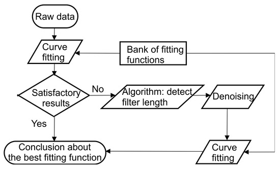
Figure 1. Preprocessing and overall process flow.

The first step in the signal processing is noise removal. Although the noise does not exist physically within the average daily fuel consumption data, it exists from the signal processing point of view. Namely, as there are sudden spikes in fuel consumption, comparing raw data would be somewhat misleading. Instead, the moving average or filtering operation is performed on raw data. The first step is to choose the size of the moving average filter (filter length). It has to be noted that ship data are not uniformly collected. Hence, there is no year, season, or month with an equal number of samples. Smoothing at the season level has been performed. The optimal filter length was identified by developing and performing an algorithm.

First, the R-square analysis of the raw data was performed. In the raw data, R-square is, e.g., 0.01636 for the Gauss 1 fitting function. As a low R-square measure implies a high noise level, raw data should be preprocessed by eliminating the noise. Since we failed to obtain satisfactory results, we proceeded according to the flow diagram given in Figure 1. First, we detected the filter length necessary for moving the average operation, and then performed the moving average to denoise the raw data and obtain enhanced input to the curve fitting operation.

The influence of filter length can be seen in the correlation matrix. The results for the length of 52 points over four years of the moving average filter are as follows (including trends):

$$\left[\begin{array}{cccc}1.0000& 0.3987& 0.3963& 0.4210\\ -0.3987& 1.0000& 0.3532& 0.3311\\ -0.3963& 0.3532& 1.0000& 0.6988\\ -0.4210& 0.3311& 0.6988& 0.9999\end{array}\right]$$

(37)

The results for the length of 12 points of the moving average filter are:

$$\left[\begin{array}{cccc}0.9999& -0.0235& -0.2615& -0.1486\\ -0.0235& 0.9999& 0.1758& 0.2552\\ -0.2615& 0.1758& 1.0000& 0.2785\\ -0.1486& 0.2552& 0.2785& 0.9999\end{array}\right]$$

(38)

The results for the length of 24 points of the moving average filter are:

$$\left[\begin{array}{cccc}1.0000& -0.2436& -0.4057& -0.2353\\ -0.2436& 1.0000& 0.2725& 0.4084\\ -0.4057& 0.2725& 1.0000& 0.5211\\ -0.2353& 0.4084& 0.5211& 1.0000\end{array}\right]$$

(39)

The closer the correlation is to 1, the higher the similarity, and the closer the correlation is to 0, the lower the similarity. As various results for the correlation matrix are obtained by using different moving average filter lengths, we implemented an algorithm for identifying the best solution (see below: Algorithm 1 for optimum moving average filter length identification).

Algorithm 1 for optimum moving average filter length identification.

for kk from 3 to 52

data1_filtered=movemean(data1,kk)

data2_filtered=movemean(data2,kk)

A = [data1(1:length(min(data1, data2)))’

data2(1:length(min(data1, data2)))’];

% alternatively zero padding can be used that all vectors have the same length.

d = (A*A’)/(N − 1);

e = d/max(max(d));

zb(k) = sum(sum(dist(e-ones(size(e)))));

end;

find(zb == min(zb))

where N = length(min(data1, data2)).

Different results were obtained for different seasons (years). An optimum filter length was used for corresponding data in further analysis.

Data are presented by years (in the first part of the research) and by seasons (in the second part of the research). Half of the data were used to generate the equation and the other half to test the prediction hypothesis.

All the calculations were performed in the Matlab application Curve fitting tool [26]. The variables of interest were input as y-data.

4. Results

The data obtained consist of 829-time samples that are not uniformly sampled. They are obtained from a single ship (5 October 2008–28 August 2012), and refer to fuel consumption in 24 h. We used the first 434 samples (two years) to obtain the fit function, while the remaining 395 samples (two years) were used for the identification of the fitting function best suited to predict future fuel consumption. Similar analysis was performed by seasons. The analysis was divided into two parts: analysis by years known as the vertical analysis and horizontal analysis, where one year was divided into four seasons, namely, summer, autumn, winter, and spring.

4.1. Analysis by Year

The correlation matrix for the first two years is:

$$\left[\begin{array}{cc}1.0000& 0.9661\\ 0.9661& 0.9361\end{array}\right]$$

(40)

From (40), it can be seen that the correlation between the first, and the second year was 96.61%. For four years, the smoothed data had the following correlation:

$$\left[\begin{array}{cccc}1.0000& 0.9600& 0.9595& 0.8379\\ 0.9600& 0.9237& 0.9231& 0.8064\\ 0.9595& 0.9231& 0.9235& 0.8064\\ 0.8379& 0.8064& 0.8064& 0.7048\end{array}\right]$$

(41)

As the lowest correlations were between the second and the fourth year, the third and the fourth, and within the fourth year itself, there was obviously a fundamental occurrence in the 4th year, as can be seen from (41). The results obtained suggest that denoised data are suitable for further research.

Table A1 indicates the coefficients obtained. As in the case of the fitting function called Rational 1/1 (16), the fit computation did not converge, Matlab stopped fitting, because the number of iterations or function evaluations exceeded the specified maximum. The results for the other fitting functions are presented in Table A2. Table A2 shows the results for years 1 and 2, where the fit was examined by SSE, R-square, RMSE, and the adjusted R-square. The table is sorted by R-square (the best on the top). Negative results denoted with “*” imply the invalidity of the model. It can be seen that the best fit (other than the smoothing spline curves) was obtained by Fourier 8. Table A3 shows the results of the prediction for various fitting functions. Table A3 is sorted by R-square in the prediction interval (the best on the top). The measure of quality is the R-square coefficient. The best result after smoothing splines was obtained by Gaussian 7.

Figure 2 and Figure 3 show examples of the results. The dots are real samples, and the full lines are the estimated curve. Since the data are obtained by non-uniform daily sampling, the x-axes are marked as “indexed time” in all figures in the Results section. Hence, the numbers on the x-axes are not time units, but the number of daily samples, which have no units. Figure 2a and Figure 3a present the first two years, denoised ($y_{12m}$), and the fitted data ($y_{\_years12\_fit}$). Figure 2b and Figure 3b show the same for years 3 and 4, and Figure 2c and Figure 3c the same for all data (four years).

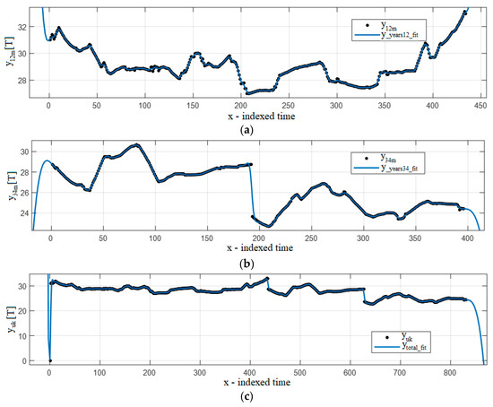
Figure 2. Smoothing spline for p = 0.309432: (a) years 1–2, (b) years 3–4, (c) years 1–4.

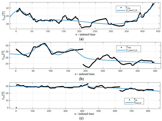
Figure 3. Gaussian 3 fitting function: (a) years 1–2, (b) years 3–4, (c) years 1–4.

4.2. Analysis by Seasons

Optimal filter length for the available data set in the summer is 21. By using the result from the algorithm, the correlation matrixes for summers 2 and 4 are:

$$\left[\begin{array}{cc}1.0000& 0.8915\\ 0.8915& 0.7984\end{array}\right],$$

(42)

$$\left[\begin{array}{cccc}1.0000& 0.9007& 0.9859& 0.8006\\ 0.9007& 0.8132& 0.8931& 0.7200\\ 0.9859& 0.8931& 0.9858& 0.7863\\ 0.8006& 0.7200& 0.7863& 0.6419\end{array}\right].$$

(43)

The obtained coefficients for the considered fitting functions are given in Table A4 (see Appendix A). As the fit computation for the Gaussian 7 function did not converge, the fitting was discontinued since the number of iterations or function evaluations exceeded the specified maximum.

The obtained measures of similarity with the fitting functions are given in Table A5, sorted by the R-square (the best on the top row). In spite of the calculation problems, Gaussian 7 yielded the best fit under the R-square criterion. Table A6 shows R-square results for the domain used to extrapolate the fitting function parameters, predicted curve, and total range, sorted by the predicted R-square domain. The Gaussian 7 fitting function could be observed to be the best fit in the prediction interval. Figure 4 and Figure 5 show examples of the results for the summer.

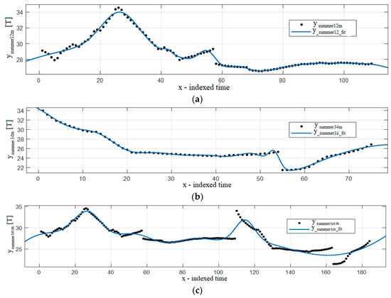
Figure 4. Gaussian 7 fitting function: (a) summers 1–2, (b) summers 3–4, (c) summers 1–4.

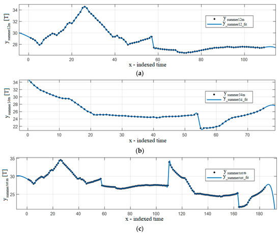
Figure 5. Smoothing spline for p = 0.9987: (a) summers 1–2, (b) summers 3–4, (c) summers 1–4.

After the summers, the analysis by season turned to autumns. The algorithm for the optimal length of the moving average filter gave the length of 42 in case of autumn. The correlation matrix for the first two autumns is:

$$\left[\begin{array}{cc}0.9734& 0.9828\\ 0.9828& 1.0000\end{array}\right]$$

(44)

In case of all four autumns, the correlation matrix is:

$$\left[\begin{array}{cccc}0.9734& 0.9828& 0.9432& 0.8338\\ 0.9828& 1.0000& 0.9557& 0.8436\\ 0.9432& 0.9557& 0.9155& 0.8088\\ 0.8338& 0.8436& 0.8088& 0.7147\end{array}\right]$$

(45)

The obtained coefficients are given in Table A7 (see Appendix A). There was a problem with the Gaussian 7 function, where the fit computation did not converge and Matlab stopped fitting because the number of iterations or function evaluations exceeded the specified maximum.

Table A8 shows the results for level of fit. Data were sorted by the R-square parameter. The best results (after the smoothing splines) were obtained by the Gaussian 8 and Fourier 7. Table A9 shows R-square for autumns 1 and 2, autumns 3 and 4, and autumns 1–4. Data are sorted by prediction interval, with the Gaussian 7 fitting function giving the best prediction (after the smoothing spline functions).

Figure 6 and Figure 7 show examples of the results, with real data illustrated with dots, and fitted curves with full lines. In this case, Gaussian 7 is chosen for Figure 6, and Rational 3/2 function for Figure 7. Figure 6b,c and Figure 7b,c show discontinuities in the middle of the graph.

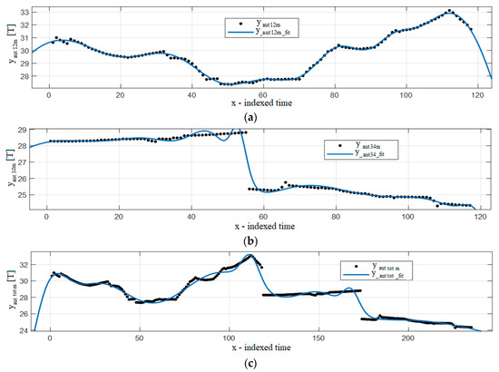
Figure 6. Gaussian 7 fitting function results: (a) autumns 1–2, (b) autumns 3–4, (c) autumns 1–4.

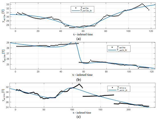
Figure 7. Rational3/2 fitting function results: (a) autumns 1–2, (b) autumns 3–4, (c) autumns 1–4.

Correlations for two winters are:

$$\left[\begin{array}{cc}1.0000& 0.9513\\ 0.9513& 0.9049\end{array}\right]$$

(46)

and for all winters:

$$\left[\begin{array}{cccc}1.0000& 0.9513& 0.9647& 0.8458\\ 0.9513& 0.9049& 0.9176& 0.8045\\ 0.9647& 0.9176& 0.9306& 0.8160\\ 0.8458& 0.8045& 0.8160& 0.7157\end{array}\right]$$

(47)

The obtained coefficients (for fitting functions) for winters 1 and 2 are given in Table A10 (see Appendix A). For the Gaussian 7 fitting function, the fit computation did not converge and the fitting was halted. The results in the table are the last obtained in this case.

Table A11, sorted by the R-square parameter, shows quality measures for winters 1 and 2. The best fit was obtained with Gaussian 7 (if the smoothing splines were excluded). Table A12, sorted by the predicted domain, shows R-squares for winters 1–2, 3–4, and 1–4. Gaussian 7 is the best for the prediction (when smoothing splines are excluded).

Figure 8 shows an example of the results in the case of the Gaussian 7 fitting function.

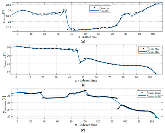
Figure 8. Gaussian 7 fitting function results: (a) winters 1–2, (b) winters 3–4, (c) winters 1–4.

In the case of the two springs, the optimal length for the moving average filter was 47. Correlations for the two springs are:

$$\left[\begin{array}{cc}0.9780& 0.9885\\ 0.9885& 1.0000\end{array}\right]$$

(48)

and for four springs:

$$\left[\begin{array}{cccc}0.8157& 0.8332& 0.9025& 0.6972\\ 0.8332& 0.8515& 0.9226& 0.7113\\ 0.9025& 0.9226& 1.0000& 0.7700\\ 0.6972& 0.7113& 0.7700& 0.5974\end{array}\right]$$

(49)

The results for two springs are given. The obtained coefficients for the fitting functions are presented in Table A13 (see Appendix A).

The results for quality measures in case of springs 1 and 2 are shown in Table A14, which is sorted by the best R-square. Better results are for rougher smoothing spline (p closer to 1), which is not favorable. On the contrary, smoother splines are welcome and the achieved results are not as good. Apart from the smoothing splines, the best result was obtained with Gaussian 7. Table A15, sorted by the best fits in the prediction interval, shows the results for springs 1–2, 3–4, 1–4. Fourier 8 was shown as the best for the prediction purposes in the case of springs.

Figure 9 and Figure 10 show examples of the results for springs. Fourier 8 clearly exhibits discontinuity around the middle of the dataset.

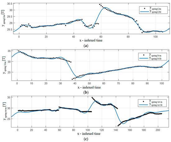
Figure 9. Fourier 8 fitting function results: (a) springs 1–2, (b) springs 3–4, (c) springs 1–4.

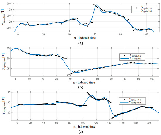
Figure 10. Gaussian 7 fitting function results: (a) springs 1–2, (b) springs 3–4, (c) springs 1–4.

5. Discussion and Conclusions

The paper presents a black-box approach to ship fuel consumption based on signal (daily fuel consumption) analysis. The real data were analyzed. The fitting function should enable the easy build in of the possible tools/software in the future, which is simple and requires low processor power. This fitting function should reflect the coupling between data and sources. Due to nonlinearities, various data were transformed to the same coordinates. This is important, because monthly, seasonally, or yearly data do not have the same length. The explored approach should include aspects of de-trending, coupling, nonlinearities, unreliable data, and different lengths of data within the same time period. Finally, the fitting function would enable the prediction of fuel consumption and differentiate it from the actual consumption. If an anomaly is detected, the company could investigate whether the cause is the weather, fouling, or even fraud. During the research, it was assumed that fuel consumption would grow linearly over time. Such dependence would make possible to use some linear regression methods (e.g., [20,29]). However, the results did not show that consumption had actually decreased, which could be associated with the following factors:

• non-uniform time sampling (leading to wrong curve angle between the interpolating points), and
• average (which depends on the route the ship was sailing at the time of data acquisition, and the sailing hours on a specific day).

It was obvious from the results of the R-square and the adjusted R-square measures that the data were not well conditioned for the correct analysis. Hence, different approaches were used. Firstly, the data were preprocessed with filters, which resulted in better R-square and adjusted R-square metrics. The next step was to use a bank of fitting functions to find the best match. Higher-order functions were observed to result in a better fit. The best functions to choose for the model were the smoothing splines, but in the so-called rougher (not smoother) versions (parameter p closer to 1), as rougher splines fit better sampling points, although they were not suitable for real-world applications. Instead, the Gaussian, Fourier or rational functions were chosen for the prediction model. In this case, the best fit of the predicted data (samples for 3rd and 4th year/season) was obtained by Gaussian, Fourier, and rational functions that generally tend to be represented by the first-order polynomial. Higher order functions tend to oscillate around the sampled data more tightly. That reduces the error, and it could lead to the conclusion that such functions (i.e., Gaussian 7) could be used in any ship by simply adjusting the function parameters, which is the advantage in our signal-based approach. The result was obtained easily and fast, which is an advantage over methods that attempt to estimate real fuel consumption by examining engine characteristics and parameters.

In the analysis, we explored comparisons between years, and comparisons between seasons. The worst correlations were obtained between the second and the fourth year, the third and the fourth, and within the fourth year itself, suggesting a relevant event of some sort in the fourth year. Likewise, the correlation between summers, autumns, and winters was above 80%. On the other hand, springs were less correlated, presumably due to the state of the ship’s hull after wintertime, and the great oscillations in weather conditions that typically occur in springtime.

Finally, there were two contributions of this paper. The main contribution, as far as the authors are aware, was that this was the first time that seasons (so called horizontal analysis) were considered for prediction purposes. A minor contribution of the paper was the algorithm for identifying the optimum moving average filter length.

The prediction formula takes into account environmental and biological influences, as well as cargo mass, and all other possible fuel consumption factors. We strongly believe that it could be used to detect potential frauds (fuel theft), which may be of interest to various authorities. Furthermore, the proposed prediction model is simple and fast to use, and can be used to check deviations in fuel consumption by comparing the predicted and deviated consumption. A deviation could be caused by fraud or by environmental factors such as fouling.

There are additional differences between this paper and references. For example, the results in [19] are obtained by excluding suspicious data in the preprocessing stage. We used all available data to obtain our results. Most of the references used a deep learning approach with ANNs [19,20,21,22,23]. On the other hand, it was not necessary to use ANNs always. It was popular, but not necessary. Hence, further research could include the identification of factors that cause unplanned fuel consumption and modeling fuel consumption by artificial neural networks (ANN) and hybrid models of velocity and fuel consumption.

References

- Marques, C.H.; Caprace, J.-D.; Belchior, C.R.P.; Martini, A. An Approach for Predicting the Specific Fuel Consumption of Dual-fuel Two-stroke Marine Engines. J. Mar. Sci. Eng. 2019, 7, 20. [Google Scholar] [CrossRef]
- Tran, T.A. Design the Prediction Model of Low-Sulfur-Content Fuel Oil Consumption for M/V NORD VENUS 80,000 DWT Sailing on Emission Control Areas by Artificial Neural Networks. In Proceedings of the Institution of Mechanical Engineers, Part M. J. Eng. Marit. Environ. 2019, 233, 345–362. [Google Scholar]
- Krčum, M.; Gudelj, A.; Tomas, V. Optimal Design of Ship’s Hybrid Power System for Efficient Energy. Trans. Marit. Sci. 2018, 7, 23–32. [Google Scholar] [CrossRef]
- Geertsma, R.D.; Visser, K.; Negenborn, R.R. Adaptive pitch control for ships with diesel mechanical and hybrid propulsion. Appl. Energy 2018, 228, 2490–2509. [Google Scholar] [CrossRef]
- Aronietis, R.; Sys, C.; van Hassel, E.; Vanelslander, T. Forecasting Port-level Demand for LNG as a Ship Fuel: The Case of the Port of Antwerp. J. Shipp. Trade 2016, 1, 2. [Google Scholar] [CrossRef]
- Tsujimoto, M.; Sogihara, N. Prediction of Fuel Consumption of Ships in Actual Seas. Available online: http://www.naoe.eng.osaka-u.ac.jp/kashi/SOEMeeting/PPT/SOE1_Tsujimoto.pdf (accessed on 5 November 2019).
- Górski, W.; Abramowicz-Gerigk, T.; Burciu, Z. The Influence of Ship Operational Parameters on Fuel Consumption. Zesz. Nauk. 2013, 36, 49–54. [Google Scholar]
- Bialystocki, N.; Konovessis, D. On the Estimation of Ship’s Fuel Consumption and Speed Curve: A Statistical Approach. J. Ocean Eng. Sci. 2016, 1, 157–166. [Google Scholar] [CrossRef]
- Lu, R.; Turan, O.; Boulougouris, E. Voyage Optimisation: Prediction of Ship Specific Fuel Consumption for Energy Efficient Shipping. In Proceedings of the 3rd International Conference on Technologies, Operations, Logistics and Modelling for Low Carbon Shipping, London, UK, 9–10 September 2013. [Google Scholar]
- Banawan, A.A.; Mosleh, M.; Seddiek, I.S. Prediction of the Fuel Saving and Emissions Reduction by Decreasing Speed of a Catamaran. J. Mar. Eng. Technol. 2014, 12, 40–48. [Google Scholar]
- Larsen, U.; Pierobon, L.; Baldi, F.; Haglind, F.; Ivarsson, A. Development of a Model for the Prediction of the Fuel Consumption and Nitrogen Oxides Emission Trade-off for Large Ships. Energy 2015, 80, 545–555. [Google Scholar] [CrossRef]
- Gheriani, E. Fuel Consumption Prediction Methodology for Early Stages of Naval Ship Design. Master’s Thesis, MIT, Massachusetts Institute of Technology, Cambridge, MA, USA, 2012. [Google Scholar]
- Pétursson, S. Predicting Optimal Trim Configuration of Marine Vessels with Respect to Fuel Usage. Master’s Thesis, University of Iceland, Reykjavik, Iceland, 2009. [Google Scholar]
- Borkowski, T.; Kasyk, L.; Kowalak, P. Assessment of Ship’s Engine Effective Power Fuel Consumption and Emission using the Vessel Speed. J. KONES Powertrain Transp. 2011, 18, 31–39. [Google Scholar]
- Demirel, A.K.; Turan, O.; Incecik, A. Predicting the effect of biofouling on ship resistance using CFD. Appl. Ocean Res. 2017, 62, 100–118. [Google Scholar] [CrossRef]
- Kan, Z.; Tang, L.; Kwan, M.P.; Zhang, X. Estimating Vehicle Fuel Consumption and Emissions Using GPS Big Data. Int. J. Environ. Res. Public Health 2018, 15, 566. [Google Scholar] [CrossRef] [PubMed]
- Zhao, Q.; Chen, Q.; Wang, L. Real-Time Prediction of Fuel Consumption Based on Digital Map API. Appl. Sci. 2019, 9, 1369. [Google Scholar] [CrossRef]
- Kee, K.K.; Simon, B.Y.L.; Renco, K.H.Y. Prediction of Ship Fuel Consumption and Speed Curve by Using Statistical Method. J. Comp. Sci. Comput. Math. 2018, 8, 19–24. [Google Scholar] [CrossRef]
- Hu, Z.; Jin, Y.; Hu, Q.; Sen, S.; Zhou, T.; Osman, M.T. Prediction of Fuel Consumption for Enroute Ship Based on Machine Learning. IEEE Access 2019, 7, 119497–119505. [Google Scholar] [CrossRef]
- Wang, S.; Ji, B.; Zhao, J.; Liu, W.; Xu, T. Predicting Ship Fuel Consumption based on LASSO Regression. Transp. Res. D Transp. Environ. 2018, 65, 817–824. [Google Scholar] [CrossRef]
- Ahlgren, F.; Mondejar, M.E.; Thern, M. Predicting Dynamic Fuel Oil Consumption on Ships with Automated Machine Learning. Energy Procedia 2019, 158, 6126–6131. [Google Scholar] [CrossRef]
- Panapakidis, I.; Sourtzi, V.-M.; Dagoumas, A. Forecasting the Fuel Consumption of Passenger Ships with a Combination of Shallow and Deep Learning. Electronics 2020, 9, 776. [Google Scholar] [CrossRef]
- Uyanik, T.; Arslanoglu, Y.; Kalenderli, O. Ship Fuel Consumption Prediction with Machine Learning. In Proceedings of the 4th International Mediterranean Science and Engineering Congress, Antalya, Turkey, 25–27 April 2019; pp. 757–759. [Google Scholar]
- Mosaic Data Science, Predicting Fuel Usage Anomalies, Case Study. Available online: http://www.mosaicdatascience.com/2018/05/11/predicting-fuel-usage-anomalies/ (accessed on 20 October 2019).
- Coraddu, A.; Oneto, L.; Baldi, F.; Anguita, D. Vessels Fuel Consumption: A Data Analytics Perspective to Sustainability. In Soft Computing for Sustainability Science; Studies in Fuzziness and Soft Computing; Cruz Corona, C., Ed.; Springer: Cham, Switzerland, 2018; pp. 11–48. [Google Scholar]
- MathWorks Inc. Curve Fitting Toolbox™ User’s Guide R2018b; MathWorks Inc.: Natick, MA, USA, 2018. [Google Scholar]
- Oppenheim, A.V.; Verghese, G.C. Signals, Systems and Inference; Pearson Education Limited: New York, NY, USA, 2016. [Google Scholar]
- Wang, Z.; Bovik, A.C. Mean Squared Error: Love It or Leave It? IEEE Signal Proc. Mag. 2009, 26, 98–117. [Google Scholar] [CrossRef]
- Botchkarev, A. A New Typology Design of Performance Metrics to Measure Errors in Machine Learning Regression Algorithms. Interdiscip. J. Inf. Knowl. Manag. 2019, 4, 45–76. [Google Scholar] [CrossRef]
© 2020 by the authors. Licensee MDPI, Basel, Switzerland. This article is an open access article distributed under the terms and conditions of the Creative Commons Attribution (CC BY) license (http://creativecommons.org/licenses/by/4.0/).