Article

A User-Oriented Local Coastal Flooding Early Warning System Using Metamodelling Techniques

1
BRGM, 45060 Orléans, France
2
Antea Group, 45160 Olivet, France
3
Institut de Mathématiques de Toulouse (IMT), 31400 Toulouse, France
*
Author to whom correspondence should be addressed.
Current address: Maître de Conférences, Université Polytechnique Haut-de-France, Céramaths, 59313 Valenciennes, France.
J. Mar. Sci. Eng. 2021, 9(11), 1191; https://doi.org/10.3390/jmse9111191
Submission received: 20 September 2021 / Revised: 21 October 2021 / Accepted: 22 October 2021 / Published: 27 October 2021
(This article belongs to the Section Coastal Engineering)

Abstract

:
Given recent scientific advances, coastal flooding events can be properly modelled. Nevertheless, such models are computationally expensive (requiring many hours), which prevents their use for forecasting and warning. In addition, there is a gap between the model outputs and information actually needed by decision makers. The present work aims to develop and test a method capable of forecasting coastal flood information adapted to users’ needs. The method must be robust and fast and must integrate the complexity of coastal flood processes. The explored solution relies on metamodels, i.e., mathematical functions that precisely and efficiently (within minutes) estimate the results that would provide the numerical model. While the principle of relying on metamodel solutions is not new, the originality of the present work is to tackle and validate the entire process from the identification of user needs to the establishment and validation of the rapid forecast and early warning system (FEWS) while relying on numerical modelling, metamodelling, the development of indicators, and information technologies. The development and validation are performed at the study site of Gâvres (France). This site is subject to wave overtopping, so the numerical phase-resolving SWASH model is used to build the learning dataset required for the metamodel setup. Gaussian process- and random forest classifier-based metamodels are used and post-processed to estimate 14 indicators of interest for FEWS users. These metamodelling and post-processing schemes are implemented in an FEWS prototype, which is employed by local users and exhibits good warning skills during the validation period. Based on this experience, we provide recommendations for the improvement and/or application of this methodology and individual steps to other sites.

1. Introduction

Approximately 600 million people live in coastal plain areas (i.e., coastal regions less than 10 m above mean sea level; [1]), which are broadly recognised as “at-risk” territories that could be subjected to significant hazards in the future, particularly with the increasing risk of coastal flooding due to sea-level rise. The flooding risk of low-lying coasts is expected to increase significantly by the end of this century (with very high confidence) in the absence of major additional adaptation efforts [2]. As highlighted by [3], effectively adapting to this rising flood risk requires a diversified approach of interventions, which may include structural flood protection measures, risk-informed land planning, nature-based solutions, social protection, risk financing instruments, and forecast and early warning systems (FEWSs).
Past flood events (e.g., Hurricane Katrina, which struck the USA in 2005, and Storm Xynthia, which impacted France in 2010) illustrate the complexity of coastal systems and the limits of traditional FEWSs and flood risk analyses. Indeed, coastal flooding is the consequence of a variety of processes (e.g., atmospheric circulations, waves, atmospheric surges, tides, river discharges) that are generated at and interact on different spatio-temporal scales; in general, local flooding, especially in urban areas, results from processes occurring at high spatial and temporal resolutions. Floods can be induced by overflow (when the total water level, including the wave setup, exceeds the coastal defence crests) and wave overtopping. Owing to the significant progress achieved in numerical hydrodynamic models (especially phase-resolving models, e.g., Simulating Waves till Shore (SWASH), [4]), it is now possible to precisely reproduce floods, even in the case of wave overtopping (see, e.g., [5,6,7]).
Focusing on coastal flood FEWSs, one of the main issues (in addition to the model skill and input data quality) of advanced flood models is the computational time. Indeed, the modelling of coastal flooding at the proper resolution (metric) to predict floods in urban areas and account precisely for processes such as wave overtopping is so time consuming (i.e., the computation time is hardly smaller than the real time) that forecasting efforts are greatly hindered. Four solutions are generally considered for this issue: (S1) high-performance computing (HPC), (S2) modelling with reduced process complexity, (S3) pre-calculated flooding scenarios, and (S4) expert judgement. For example, numerous FEWSs do not model floods and instead rely on expert judgement. Ref. [8] provides an example of such an approach. In France, the national FEWS (the Vigilance Vague Submersion (VVS) system operated by Météo-France) provides warnings at a department scale, relying on coastal hydrodynamic forecasts of different sources and a threshold decision matrix (wave height and still water level) calibrated on past flooding events (solution S4). However, this approach has limits when facing conditions that have never occurred or have never been observed and could lead to a significant number of false alarms, which could reduce the confidence in and reactivity to warnings if they are triggered too frequently (colloquially known as “crying wolf”). Even if 100% of all warnings are accurately predicted, such a system does not provide inland flood information, and whether a particular asset will still be operational or accessible during a flood event cannot be predicted.
In contrast, FEWSs relying on solutions S1, S2, or S3 provide model-based flooding information. For instance, the Coastal and Inland Flooding Observation and Warning (CI-FLOW) demonstration project for coastal North Carolina relies on models using the shallow-water equations [9]; nevertheless, while this approach is well-suited to overflow events, it is not adequate for overtopping. In the UK, employing some simplifications and expecting that HPC will allow their integration into operational systems, developments have allowed flood predictions to account for both overflow and overtopping [10]. In the Netherlands, the issuance of warnings by the operational FEWS is based on forecasted nearshore conditions (as in other FEWSs); in the case of a warning, the flood is estimated using a database of pre-calculated flooding scenarios for a pre-defined set of dike breach locations and water levels with a model resolution of approximately 10 m (personal communication). One of the limits of this approach is that it is limited to pre-defined scenarios. Furthermore, even in such advanced systems, the complexity of flooding processes and the variety of possible events are not fully taken into account. Other FEWSs predict flood-related information (e.g., the occurrence of overtopping events) but do not truly provide predictions for inland floods (see, e.g., [11,12] for overtopping forecasts). However, these FEWSs operate by modelling overtopping phenomena on cross-shore profiles; while this approach may be sufficient for warnings, it cannot deduce the spatial characteristics of inland floods, especially along non-uniform coasts, where the location of the modelled profile is critical when predicting inland floods.
At the same time, significant progress has been achieved in the use of artificial intelligence for flood prediction. For instance, data-driven machine learning techniques are widely used for continental flood prediction [13,14,15,16]. These approaches rely on observational datasets (typically from water-level sensors installed in rivers and others channels) that are relatively large (for instance, comprising hourly measurements at several locations over several months or years). However, the characteristics of coastal domains are quite different: inland sensors are typically lacking, with the exception of smart cities such as Macao [17], and while tide gauges are occasionally available, these types of measurements are not sufficient to deduce coastal flood information (e.g., the flood extent or inland water depth), especially on sites subject to wave overtopping. The alternative is to rely on hydrodynamic models to build learning datasets. However, the computation time of such models significantly limits the number of runs/scenarios; as a result, the statistical method being used must be adapted to the scarcity of the dataset. In recent years, metamodelling techniques have been explored for coastal hydrodynamics and coastal water level predictions and have shown promising results (e.g., [18,19]). Metamodels (also called surrogate or response models; for an introduction, see [20]) are functions that aim to reproduce the behaviour of a “true” model (e.g., a numerical hydrodynamic model) for given input variables (for instance, offshore conditions). In addition, as highlighted by [21], FEWSs should be user-centred and not designed following the linear paradigm of model-based FEWSs (i.e., a linear set of connections from observations to the generation of warnings and their transmission to users).
To better explore the potential of metamodelling techniques for coastal flood FEWSs, the ANR RISCOPE project was initiated in 2017 with the aim of establishing a user-centred FEWS by relying on metamodelling techniques. This project led to the development and exploration of metamodels and their ability to predict information regarding inland floods [22,23,24]. Within this project, Ref. [25] provided a preliminary overview of the FEWS setup methodology, from the identification of user needs to the FEWS interface.
Building on the results of these previous investigations, the present manuscript describes the establishment of a local FEWS that can predict coastal floods up to 3 days in advance while relying on the metamodelling solution whose goal is to directly predict the information of interest for local users. The novelty of the present work is to tackle the entire process, from the identification of user needs to the deployment of the fast-running FEWS and its validation. A side objective is to investigate whether the needed elements (data, models, etc.) are adequately mature to allow the prediction of local floods with good confidence. The FEWS is developed in Gâvres, France. We first describe the materials and methods (site, indicators, numerical model, metamodel, and FEWS elements). Then, we present and discuss the results (learning dataset, metamodel skills, and FEWS skills). Finally, we discuss future challenges and provide some recommendations. All the abbreviations and acronyms used in the present manuscript are listed in Acronyms and Abbreviations.

2. Materials and Methods

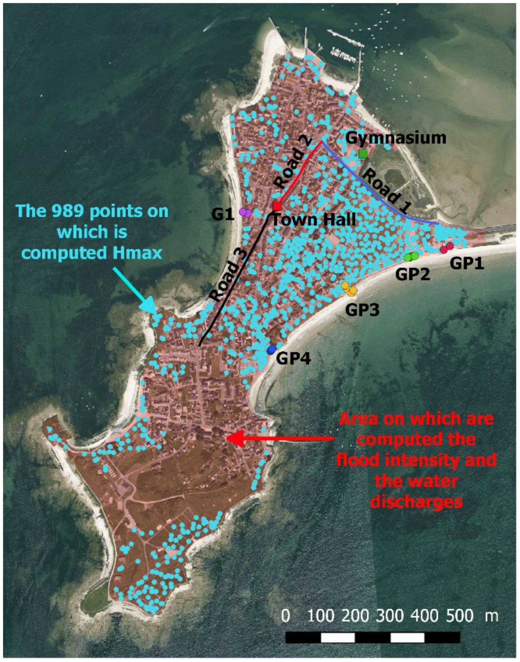
2.1. Site Description: Physical Setting, User Practices and Needs

The site of Gâvres, located on the French Atlantic coast (Figure 1a), was selected as the demonstration site for the following reasons. First, this site experienced 5 significant past flood events since 1900 (see [7] for a detailed analysis over the period 1900–2010). The last major flood occurred on 10 March 2008 (Windstorm Johanna). This implies that the local actors in coastal flood risk management have a minimum level of risk awareness, knowledge, and practice. During this last major flooding event, approximately 120 houses were flooded (Appendix A, Figure A1, purple dots). This flood was mainly related to wave overtopping processes [5,26]. Keeping in mind that the precise modelling of wave overtopping is more complex and computationally time consuming than that of overflow, Gâvres makes for a very challenging demonstration site but is representative of all the towns presently subject to wave overtopping. Finally, Gâvres (with a surface area of only 2 km2) is a small territory; hence, within our exploratory work, the interactions with the potential users of the FEWS are more manageable, and coastal flood modelling can account for wave overtopping phenomena (see Section 4.2 for further details).
In brief, Gâvres is located in a macro-tidal environment (mean spring tidal range: 4.2 m) and is subject to significant infragravity waves [27]. The coastal waves in this region are affected by the presence of an offshore island (Groix) located west of the study site (Figure 1a); as a consequence, the offshore wave conditions between the site and Groix are strongly non-uniform. Some wave modelling tests (not shown) show that the local non-uniform wave conditions result mainly from the propagation of wave conditions observed south of Groix (Figure 1a, grey star).
To identify the local practices and user needs, two user workshops were organised in 2017 and 2019 for representatives of the municipality of Gâvres, the emergency services of the department (SDIS56), the Lorient Agglomeration to which Gâvres belongs, and the Departmental Directorate of Territories and the Sea (DDTM56). The workshops indicated that the local practice is to (1) rely on official flood warnings (i.e., the VVS warnings issued by Météo-France at the department scale) and (2) conduct a local survey at 5 locations as soon as forecasted storms originating from the southwest coincide with a high spring tide. One of the participants also used wind, wave, and water level forecasts provided by the windguru (https://www.windguru.cz/, accessed on 15 July 2021) and Modelling and Analysis for Coast Research (MARC)-Physical and Space Oceanography Laboratory (Laboratoire d’Océanographie Physique et Spatiale, LOPS) (https://marc.ifremer.fr/, accessed on 25 July 2021) platforms. Table 1 lists the main local needs (identified during the workshops) that our FEWS prototype aims to address.

2.2. Methodology

The FEWS prototype aims to provide flood information for the next 6 tides by focusing on what happens between 3 h before and 3 h after each high tide. A longer lead time (e.g., 5 days) would exhibit significantly larger uncertainties because the quality of meteorological forecasts significantly decreases for lead times exceeding 3 days (see, e.g., [28]).
Based on our knowledge of the local needs (Table 1), the methodology we used to build this FEWS relies on the following steps:
Define the indicators (Ij, with j = 1:N) (Section 2.3);
Set up the process-based model that will be used to build the learning dataset for the metamodels (Section 2.4);
Build (and validate) the metamodels Yi = fi(X) (with i = 1:M) that are needed to estimate the indicators Ij (j = 1:N) (Section 2.5);
Implement the post-processing of the metamodel outputs (including the computation of Zk indicators) to estimate the indicators Ij (Section 2.6); and
Deploy the FEWS, which downloads the forecasted conditions X and returns the indicators Ij (j = 1:N) for the next 6 tides (Section 2.7).

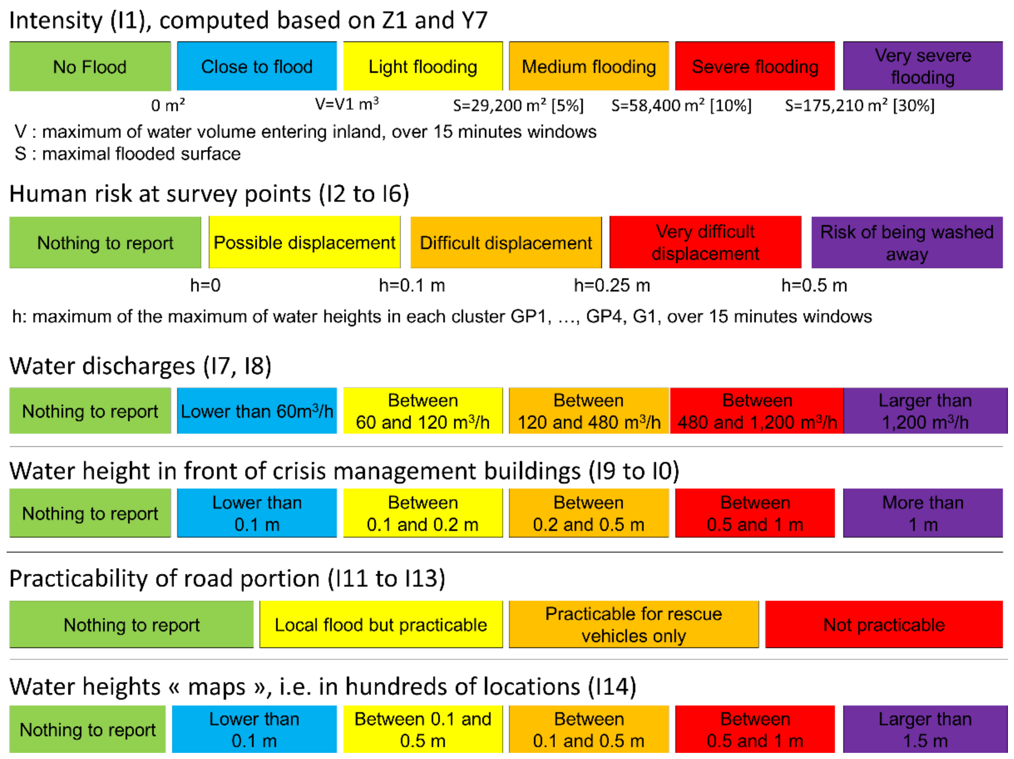
2.3. Indicators and Classes

Table 1 shows the conversion of the user needs into 14 indicators Ij, with j = 1:14. Other indicators may have been considered, such as the trafficability on every road or the water depth at each building. However, in the present research work, we first aim to test the skills of the entire process in predicting different types of information. Thus, we focus on the most critical indicators for each type of need (e.g., for the roads, the parts affecting crisis management buildings; for the buildings, only the crisis management buildings). In the list of Table 1, some indicators have no units, and others are physical quantities. Regardless of the type of indicator, one important issue when building an FEWS is that the provided information can be directly interpreted. Thus, even for indicators referring to physical quantities, instead of providing a quantitative value, we provide the class in which the indicator falls. These classes are defined in different ways depending on the indicators. Figure 2 and Figure 3 show the locations of the physical quantities on which each indicator is based and the associated classes, respectively.
Most of the classes (denoted C) of the indicators have been defined beforehand based on the literature, national recommendations, and local specific requests. For instance, for the human risk at survey points (I2–I6), we rely on studies of the loss of human stability as a function of the water depth and velocity (see, e.g., [30]); moreover, as these survey points are located either on coastal defences or on the upper beach, we assume that the velocity is greater than 1 m/s when water is present. This assumption is confirmed by analysing the results obtained with the numerical model presented in the next section. For the classes of the maximal water height (I14) over the tide, at the 989 points, we rely mainly on the national flood hazard recommendations [31], and we include the 0.1 m class, as this threshold of 0.1 m is important for emergency services. This approach allows us to provide information with which the users are familiar, as they are used to seeing flood hazard maps. For the water discharge (I7 and I8), the classes are built based on the capacities of the available pumping engines of the emergency service (SDIS56, which is located outside Gâvres) to help them plan which types of engines they should bring to the site before the flood. For the intensity (I1), 6 classes are defined based on thresholds of the flooded surface (percentage of the area: 5%, 10%, 30%), thereby ensuring that the Johanna-induced flood (10 March 2008), the last major flooding event to affect the demonstrate site (see Figure A1 in Appendix A), falls in the high-intensity class. An additional class is included to distinguish events where only few waves overtopped the coastal defences from real flood events. It is important to note that the colour scale in Figure 3 is indicator specific, i.e., that just because indicator I2 would fall in the higher (purple) class does not mean that the other indicators should fall in their higher classes. Indeed, I2–I6 focus on human risks, while the water discharge classes are designed based on the pumping engine capacities, and I1 focuses on the intensity of the flood over the entire territory.
Finally, to compute each indicator, we rely on the computation of quantities (called Yi, with i = 1:N) predicted with metamodels. Table 2 provides a list of these metamodels and for which indicator Ij they are used. Metamodels Y7 to Y18 are designed to use functional inputs (i.e., time-varying forcing conditions), while metamodels Y1 to Y6 use scalar inputs (i.e., steady forcing conditions). Indeed, metamodels Y1 to Y6 aim mainly to predict whether water will enter inland (Y1) or to predict the water depth on the upper part of the beach/coastal defence (Y2 to Y6); hence, we can use these metamodels to make quasi-steady computations, i.e., discretise the time window of interest (here, (HT − 3 h:HT + 3 h), with HT referring to high tide) in smaller windows and perform computations with steady forcing conditions in each sub-window. For the road practicability (I11–I13), a decision tree is used, where the threshold is defined by the fording depths of the considered cars (e.g., 0.3 m for passenger cars and 0.6 m for emergency vehicles; [29]).

2.4. Process-Based Model Setup and Validation

In the present study, the model has to account for both wave overtopping and wave overflow processes. Several coastal flood modelling approaches have been developed to include such processes (for a review, see [32]). One approach is to use empirical (e.g., Eurotop; [33]) formulas to estimate the wave overtopping volume along 1D cross-shore profiles based on the water level and wave conditions at the toe of the coastal defence and to use these volumes as the forcing conditions for the shallow-water models, for instance, to compute the inland flood propagation. However, these formulas have some limits, including the fact that they were designed for specific hard defences and thus are not adapted to the natural environment or nonclassical coastal defences [33]. In these cases, one solution is to use phase-resolving wave models (see, e.g., [4,34]) to compute the wave overtopping volumes along a limited number of 1D cross-shore profiles (see, e.g., [35]). However, this approach is sensitive to the locations of the profiles along which the wave overtopping discharges/volumes are computed. An alternative, albeit one that is much more computationally intensive but better accounts for the complexity of the processes (especially at a site such as Gâvres, which is not uniform in the alongshore direction), is to use the same type of phase-revolving models in 2D or 3D mode on a spatial grid covering the nearshore and inland domains (e.g., the domain illustrated in Figure 1b).
In the framework of the present study, we follow the last approach mentioned above and use the non-hydrostatic phase-resolving model SWASH [4,36] to model floods at the study site (Figure 1b). The modelling chain was previously set up by [6,7]. We briefly summarise the key elements here. First, the wave conditions off the shore of Groix (the significant wave height Hs, peak period Tp, and peak direction Dp) are downscaled to the boundaries of the SWASH model (Figure 1b) using the WW3 spectral wave model [37] by adopting the Jonswap wave spectrum with a directional spread of 30° and taking into account the local wind (wind intensity U and wind direction Du) and still water level (SWL; including the mean sea level (MSL), tide (T), and atmospheric surge (S)). The WW3 computation domain is shown in Figure 1a (in black). SWASH is run with non-uniform wave boundary conditions and spatially uniform still water levels (spatially uniform mean sea level, tides, and atmospheric surges) and local wind. The spatial and temporal resolutions of SWASH are 3 m and >10 Hz, respectively. In the vertical direction, a discretisation of two layers is used. This model chain has been validated in terms of the flooded area during the 10 March 2008 event [6]; for this validation, the model was run for a DEM representative of the 2008 period (denoted DEM2008). Appendix A shows the reasonable agreement between the modelled maximal inland water depth during the event and the observed flood extent (flooded houses). In addition, a validation of the simulated nearshore high-frequency (f > 1 Hz) water levels has been performed under more moderate conditions, showing good agreement with in situ measurements for both gravity and infragravity bands [27]. The spatial changes in the bottom roughness (related to land use) are also taken into account following the same approach as in [5].
For the present study, as the topo-bathymetry has significantly changed since 2008 due to the heightening of some coastal defences. We use the above-mentioned model chain, but we include a DEM that is as representative of the present-day configuration as possible. From the available bathymetric surveys (SHOM, DHI), lidar data (the public RGE ALTI IGN product and limited access data of the Lorient Agglomeration), and Global Positioning System (GPS) survey of the coastal defences, we have constructed a DEM (denoted DEM2015–2018) that is representative of the 2015 bathymetry (winter) and 2018 coastal defences.
In addition, Ref. [6] highlights the significant effect of the stochastic character of waves on floods at the study site, i.e., that the same offshore wave spectrum leads to different instantaneous waves and to different volumes of water entering inland. This effect is shown to be important, especially under conditions close to overflow or for events leading only to minor floods. This implies that in an FEWS where we aim not only to provide inland flood information but also to detect flood events (i.e., to distinguish floods from non-flood events) and estimate human risks on the upper beach (the survey points), it is crucial to account for this stochastic character of waves. For a given still water level, in the SWASH model, the generation of instantaneous (i.e., high-frequency) water level time series from a single wave spectrum is based on the modification of the phases of the components in the Fourier space; this is feasible owing to the user parameter named seed. Replicating simulations with different seed values allows the generation of different time series. Thus, it is possible to account for the effects of the stochastic character of waves on floods by randomly selecting the seed number in each simulation and repeating this simulation several times. However, accounting for this effect in metamodels (1) leads to an exponential increase in the number of numerical simulations and (2) requires some specific techniques. Thus, to tackle this issue, two types of metamodels are built: (1) one accounting for the effects of this stochastic character of waves (this concerns Y1–Y6) and (2) another focused more on estimating the inland impact. To support the learning of these two types of metamodels, two types of numerical simulations are performed: (Sim1) simulations on 15 min (+spin up) with scalar (i.e., steady) forcing conditions X that are repeated 20 times each with randomly selected seed values and (Sim2) simulations on 6 h (+spin up) with functional (i.e., unsteady) forcing conditions X and a constant seed value. These two types of simulations are performed for hundreds of scenarios (see Section 2.5.2). Then, the numerical results (spatio-temporal fields of the water height and velocity) are post-processed to provide the Yi values. It should be noted that except for Y2–Y6, which are computed using a 1 s sampling (numerical) model output, all the other Yi values are computed based on 1 min sampling outputs.

2.5. Metamodels

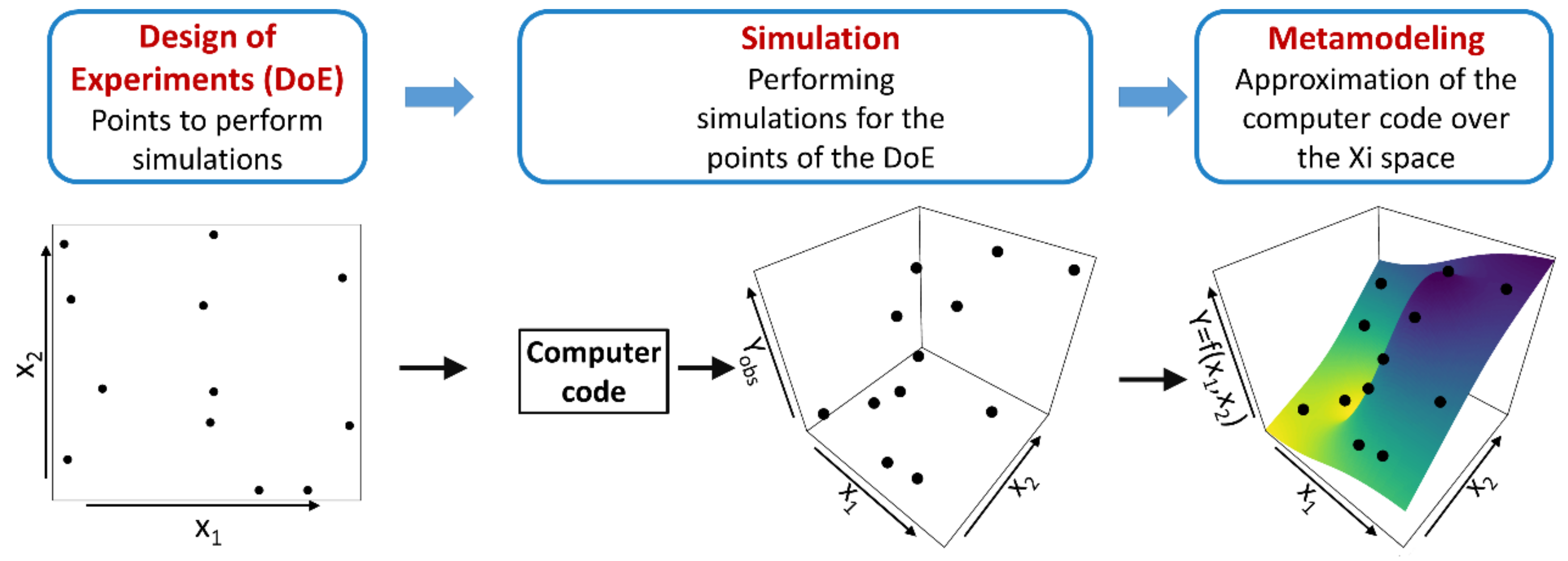
2.5.1. Principles of Metamodelling

Metamodels (also called surrogate or response models; for an introduction, see [20]) are functions that aim to reproduce the behaviour of a “true” model function f of a vector X of input variables (for instance, offshore conditions). In the present case, the “true” model is the numerical hydrodynamic model. Figure 4 illustrates the main steps involved in the construction of a metamodel. When constructing a metamodel function, first, a set of input vectors X1,…, Xn (a design of experiments) is obtained. Second, the corresponding set of output values f (X1),…,   f (Xn) is computed. The second step requires the “true” model to be evaluated n times, so n may be limited to a small value (10 to 100, for instance). Finally, the metamodel is a function f ^ of X defined on the input space covered by X1,…, Xn and learns from f (X1),…,   f (Xn). There are many standard methods for constructing a metamodel, such as linear or polynomial regression, polynomial chaos expansion [38], Gaussian processes (GPs) [39], random forests (RFs) [40], and kernel smoothing [41]. The common desirable feature among these methods is that evaluating f ^ (X) does not require calling the “true” model and has a negligible computational cost (within a few minutes). Hence, analyses that would be too costly to apply directly to the “true” model (for instance, the Monte Carlo propagation of uncertainty studies or the estimation of sensitivity indices, both of which typically require thousands of function calls to yield meaningful results) may be applied to the metamodel function instead.

2.5.2. Design of Experiments

We start by selecting a limited number n = 100 of offshore meteo-oceanic scalar conditions X = (SWL, Hs, Tp, Dp, U, Du), as was performed by [22]. This selection (S1) is designed by applying the clustering procedure described by [42] to a large dataset of extreme conditions (here, ≈150,000). This database is constructed through a combination of Monte Carlo random sampling and multivariate extreme value analysis performed on the database of hindcast conditions constructed by [7] over the period 1900–2016. This approach ensures that the selected X input conditions are sufficiently extreme to lead to flooding but are also realistic.
Then, using this first selection S1 (n = 100) and the 1900–2016 hydro-meteorological dataset [7], a probabilistic classifier is used to locate the time instants of these maximum values (based on quadratic discriminant analysis; [43]), and a multivariate Gaussian Monte Carlo-based sampling procedure is applied to generate 94 time series (S2), i.e., functional inputs X = (NMR(t), T(t), S(t), Hs(t), Tp(t), Dp(t), U(t), Du(t)) over 6 h, with 10-minute time steps. This functional input dataset is complete with 21 historical events (9 flood events and 12 non-flood events; see [7], for more details on the historical floods) and 16 scenarios simulated from small variations of the 9 historical flood events. Thus, the final grid experiment of time-varying forcing conditions contains 174 scenarios.
Regarding the scenarios of the offshore meteo-oceanic scalar conditions, the initial S1 selection is complete with 44 high tide conditions extracted from the S2 selection such that the design of experiments for the steady forcing conditions (i.e., the scalar inputs for simulation type Sim1) now contains n = 144 offshore meteo-oceanic scalar conditions X = (SWL, Hs, Tp, Dp, U, Du).

2.5.3. Metamodelling Technique

In principle, many approaches can be utilised to set up a metamodel (for an overview, see [40]), including GPs, neural networks, or support vector regression. For the present work, we select GP metamodels because they have shown very high predictive capabilities in previous applications for coastal flood assessments (among others, see [44], for applications to overflow-induced marine flooding; see [19,45], for applications to hurricanes; and see [46], for an application to San Francisco Bay). In particular, high performance was shown by the extensive comparison exercise conducted by [47]. The authors benchmarked GPs, neural networks, and support vector regression and showed that the GP outperforms the alternatives because of its lower sensitivity to the training set size. From an operational perspective, the advantage of the GP is that it acts as an exact interpolator of the simulation results and provides an estimate of the metamodel error; moreover, the GP method is parameterised by a covariance function (or kernel), which makes it flexible and allows the exploitation of expert knowledge related to the physical processes.
In the present work, for the scalar inputs, we follow the approach of [22]. A GP-based metamodel is used to predict Y1–Y6. To improve the prediction of the cases without flooding (i.e., Y1 = 0), the GP-based metamodel (see, e.g., [39]) is combined with a classification RF model [48], which aims at predicting the probability of flooding Pf (i.e., Y1 > 0). When Pf is predicted to be below 50%, the predicted value of Y1 is set to zero. Further details are provided by [22], who applied this approach using the same numerical modelling chain but with a different grid experiment and DEM2008 instead of DEM2015–2018.
A GP-based metamodel is also used for metamodels forced by functional inputs but provide scalar outputs (i.e., Y7–Y18). To reduce both the memory and the processing requirements of the metamodel, we implement the B-spline [49] and principal component analysis (PCA) [50] dimension reduction techniques, as thoroughly explained in [23], who tested this method using a simplified flood model (relying on the use of an overtopping formula over a single cross-shore profile). Compared to alternative dimension reduction approaches such as the polynomial or Fourier bases of functions, one advantage is that the basis functions from PCA are orthogonal, and those from B-splines have many zero scalar products, which can be beneficial for least square procedures when the decomposition dimension is large. In many studies, the structural characteristics of the metamodels are chosen beforehand (e.g., PCA decomposition in [51], B-spline decomposition in [52], the Matérn 5/2 covariance function in [53]) without a specific sensitivity analysis or benchmarking. In the present work, we use the ant colony-based optimisation algorithm ACO-Gp proposed in [54] to fix several structural characteristics of each metamodel, such as the set of inputs to use for prediction and the type of kernel function of the model. This algorithm helps to efficiently explore the space of potential metamodel configurations while optimising the prediction quality. Implementations for functional input GP-based metamodelling and structural optimisation supported on ACO-Gp are available through the R [55] funGp package [56], which is freely accessible from CRAN at https://cran.r-project.org/package=funGp and GitHub at https://github.com/djbetancourt-gh/funGp, accessed on 25 July 2021. Alternatives to ant colony-based optimisation could be other methods for combinatorial optimisation, such as simulated annealing or genetic algorithms. Here, ant colony-based optimisation is adapted to the tree structure of the decision space (see [54]). For instance, whether a functional input is active affects the dimension of the rest of the decision parameter to be selected. This tree structure is naturally exploitable with the pheromone paths of ant colony-based optimisation, whereas it is much less clear how to exploit this tree structure with simulated annealing or genetic algorithms.
Finally, to account for spatial outputs (as for metamodel Y18), we rely on the work of [24], the method of which is summarised as follows. Y(X,s) depends on both hydro-meteorological conditions (functional inputs) X and spatial coordinates s = (longitude, latitude). For the GP-based metamodel, we place a (zero-mean) GP prior on Y, where (1) the covariance function k is given by the separable kernel k((X,s), (X′,s′)) = kX(X,X′)ks(s,s′) and (2) the sub-kernels kX and ks evaluate the correlation between the functional inputs (X,X′) and that between the spatial coordinates (s,s′), respectively. Since k is attenuated by the spatial correlation, nearby values X and X’ can result in small correlations for distant values of s and s′, and vice versa. As Y is GP-distributed, the predictions can be performed then for classical GP-based metamodels (see, e.g., [39]). Furthermore, using a separable kernel considerably eases the implementation. As shown by [24], the resulting GP model can also be written as a multi-output model where the outputs are driven by a given set of functions. Implementations in both Python and R are freely available at https://github.com/anfelopera/spatfGPs, accessed on 25 July 2021. In the present work, we use 1003 spatially designed points. Those points are selected based on a dedicated k-means-based methodology accounting for both the spatial locations (i.e., longitude, latitude) and the flood ratios (see Section 3.1 and [24], for a further discussion). For a comparison with the more classic multi-output GP method based on linear models of coregionalisation, see also [24].

2.6. Requirements, Combination Rules of the Metamodel-Based Predictions, Optimisation, and Validation Procedure

The main requirements of the flood forecasts and warnings in our FEWS are that the system properly detects/predicts the major flooding events and minimises false alarms (i.e., properly discriminates between flood and non-flood events).
In this work, two complementary metamodelling approaches are used: one based on classification (and accounting for the effect of the stochastic character of waves) and the other based on GPs. Such a strategy allows the advantages of both approaches to be combined, especially in tackling the problem encountered by GP metamodels close to 0 (they hardly capture exact 0 values; see, e.g., [57]). Thus, to predict the indicators, the classification-based Y1 metamodel is used to force the indicators relying on the GP-based metamodels to 0 (i.e., class 1) when Z1 = 0, with Z1 being the maximum of Y1 over the tide. In addition, Z1 is used to discriminate between events at the flood limit (i.e., few wave overtopping events may occur; Z1 < V1) and events corresponding to minor flooding (Z1 ≥ V1) such that if Z1 < V1, then the intensity (I1) falls in the second class (Figure 3). At this stage, the threshold V1 is not defined; this is accomplished by optimising the numbers of true and false alarms (Section 3.3). For this optimisation step, we employ a damage database covering the period 1900–2010 together with the oceanographic forcing database [7]. These corrections can be seen as hierarchical constraints (Figure 5). In addition, some physically logical constraints are considered. For instance, the locations of indicators I9 (town hall), I10 (gymnasium), and I12 (road2) are such that they cannot be flooded if the intensity of the flood is too small (typically for Z7 < S1 with S1 = 29,200 m2, S1 corresponding to the upper limit of class no. 3 of intensity indicator I1, Figure 3). This has been checked by analysing the numerical model results for the grid experiment (see Section 3.1). Thus, an additional constraint based on Z7 is imposed to improve the prediction of indicators I9, I10, and I12. For I9 and I10, an additional constraint is imposed: if Z10 < H1 (with H1 = 0.01 m), then C(I9) = 1 considering that 1 cm of water is included in the model uncertainties. We also have knowledge of some physical relationships between a few indicators. This knowledge is taken into account, again relying on the reliability of Z1 (Figure 5, bottom-left insert). Finally, in terms of visualisation in the FEWS, indicators I7, I8, and I14 are shown only if the flood intensity triggers a flood alarm, i.e., only if C(I1) ≥ 3. The predicted indicators Ij are validated for the period from September 2019 to March 2021 (Section 3.4).

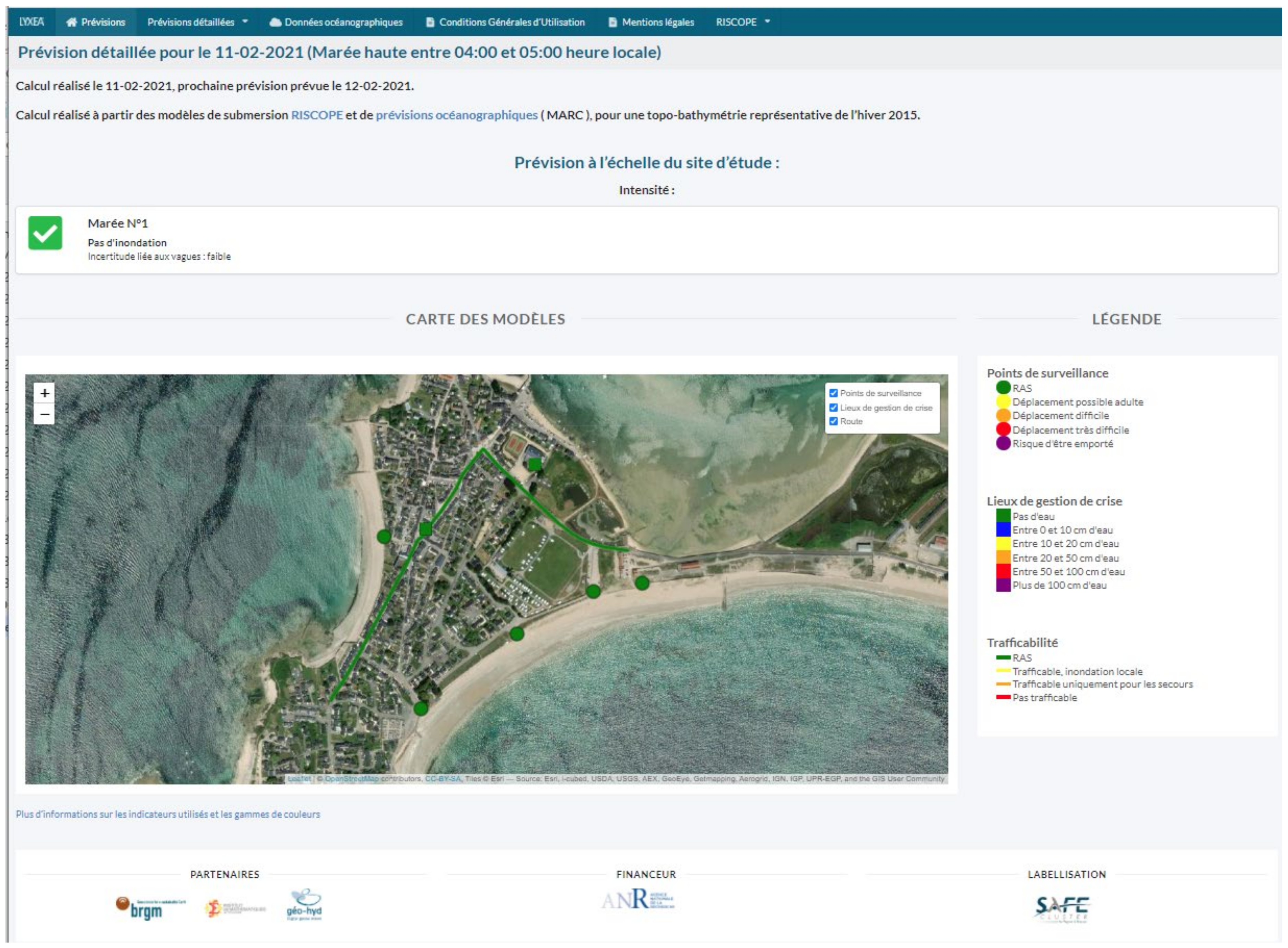
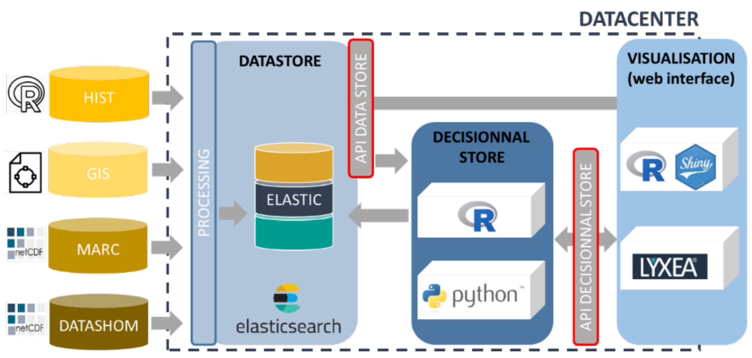
2.7. Implementation in an FEWS

The main objective of an FEWS is to provide flood information on specific targets in the area (i.e., the classes in which each indicator Ii falls) over the next six tides. This requires the use of forecasted data X. The FEWS relies on the X forecasted data provided by the MARC (https://marc.ifremer.fr/, accessed on 15 July 2021) and DATASHOM (https://data.shom.fr/, accessed on 15 July 2021) platforms. These X data are pre-processed by extracting the data at the location of interest (Figure 1a), harmonising the time steps between the different variables originating from the data suppliers (the tide T, atmospheric surge S, wave height Hs, wave peak period Tp, wave direction Dp, wind speed U, and wind direction Du). A unified time step of 10 min is used to properly account for the tide-induced sea-level variations. In a second step, the automatic detection of high tides is performed on the dataset, and then, the X data are extracted over the 6 h windows centred on the high tides for the 6 next tides. Then, the metamodels (Yi,i=1:18) are run, providing the 18 outputs for each tide. These outputs are post-processed (providing Zi,i=1:15) and aggregated into the specific indicators (Ii,1:14). Finally, the Ii indicators are published through the FEWS.
Another related objective was to provide simple figures and outputs through the FEWS. This ambition is fulfilled not only by showing the classes in which each indicator falls rather than the indicator values but also by designing an interface as simple as possible (based on user feedback).
From a technical point of view, the FEWS relies on open-source technologies, while the predictions and complementary information are provided through a website (Figure 6). The background of the FEWS is based on big data technologies that allow the storage of a large amount of data and increase the speed at which data can be visualised. More precisely, the FEWS relies on the Elasticsearch engine [58], which is a highly scalable open-source full-text search and analytics engine that allows the rapid and near-real-time storage, search, and analysis of large volumes of data. The computational aspect of the FEWS relies on Python and R (the metamodels are built using R), and R Shiny [59] is utilised to visualise the predictions. Finally, the Lyxea© software suite supports the FEWS web platform. To guarantee the scalability and shareability of the system, dedicated application programming interfaces (APIs) have been developed for the data processing chain. Finally, the accessibility of the FEWS is restricted to the members of the consortium and the final beneficiaries (the local user group) via secured access.

3. Results

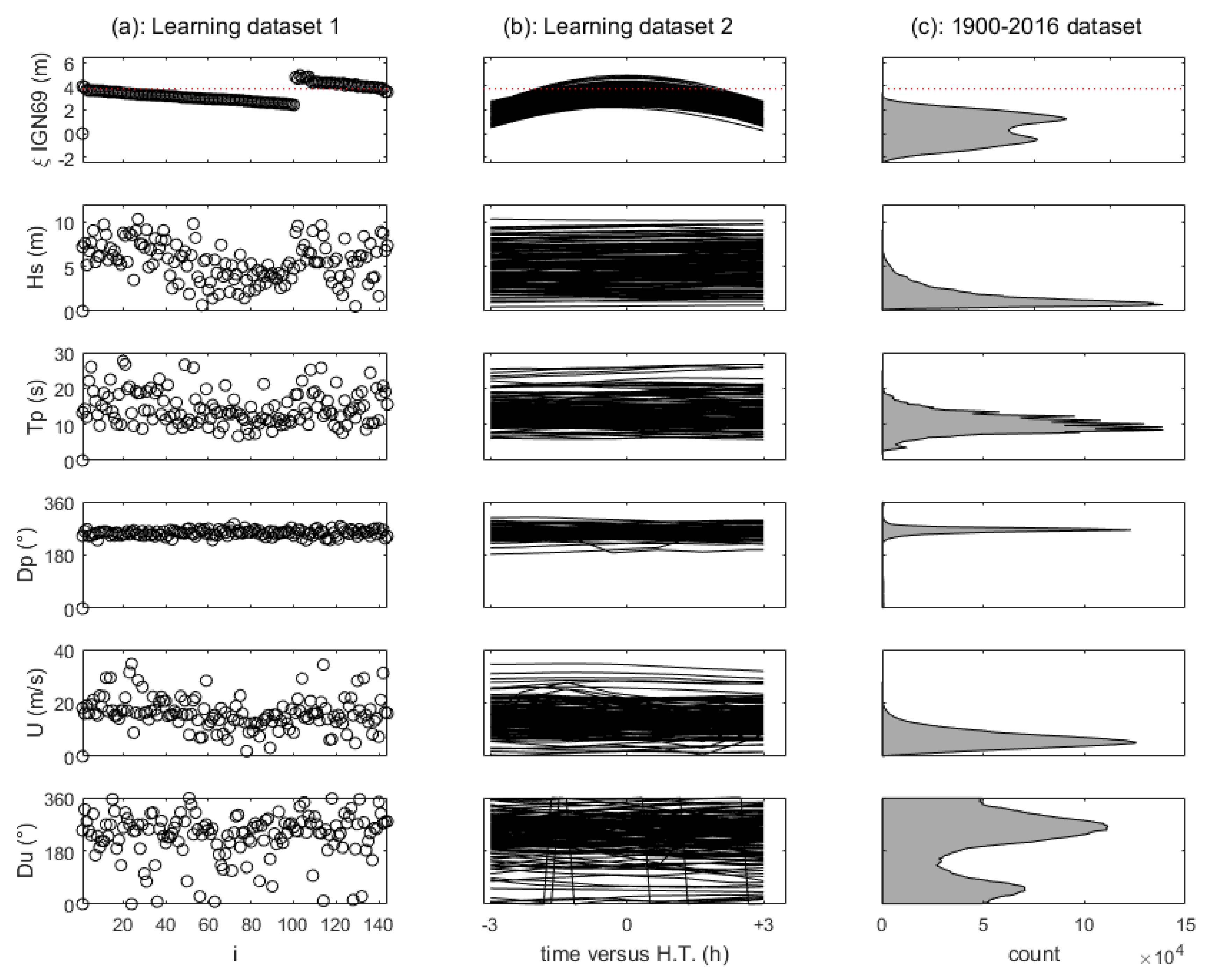
3.1. Grid Experiment and Numerical Modelling Results: Preliminary Analysis

Figure 7 illustrates the scenarios (learning dataset) that were run with the numerical model to build the scalar input metamodels (panel a) and the functional input metamodels (panel b) in comparison with the distribution of the continuous time series of X over 1900–2016 (panel c). This comparison illustrates how the grid experiment covers the X input space, which covers the distribution of the 1900–2016 X hindcast and includes past extreme events. Figure 7 further shows that the learning dataset effectively incorporates more extreme events than those observed.
From the numerical modelling, the “Y” values are extracted (denoted YNum for the Y values extracted directly from the numerical results, i.e., to avoid misunderstanding with the Y metamodels); these are the (X,YNum) datasets used to build the metamodels. The cross-validation figures provided in the next section illustrate the domain covered by YNum in comparison with the defined indicator classes. As a preliminary analysis of the numerical results, for the scalar (functional) input grid experiments Sim1 and Sim2 defined in Section 2.5.2, numerical modelling indicates that floods occur (i.e., water enters into the inland domain of analysis) in 105 (155) scenarios out of the total number of scenarios, i.e., 144 (174). Thus, the functional inputs include fewer cases without floods than the scalar inputs. Regarding the numerical results obtained from the functional input grid experiment, the ratio of the number of scenarios where the pixel is flooded to the total number of scenarios is mapped (Figure 8), illustrating the range of flood events (in terms of the flooded area) covered by the numerical simulations: from non-flood events to severe flooding (with a computed maximal flooded surface area of 312 309 m2, i.e., 55% of the studied area).

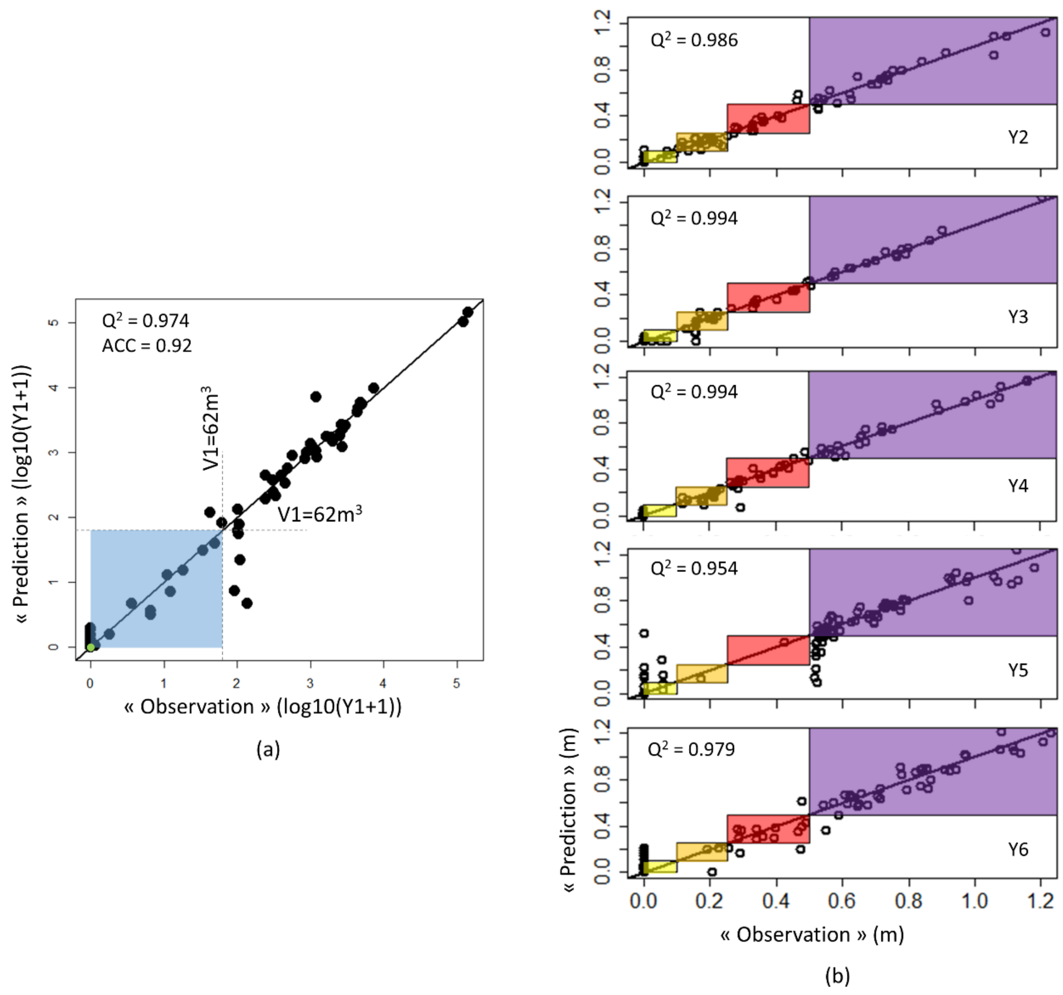
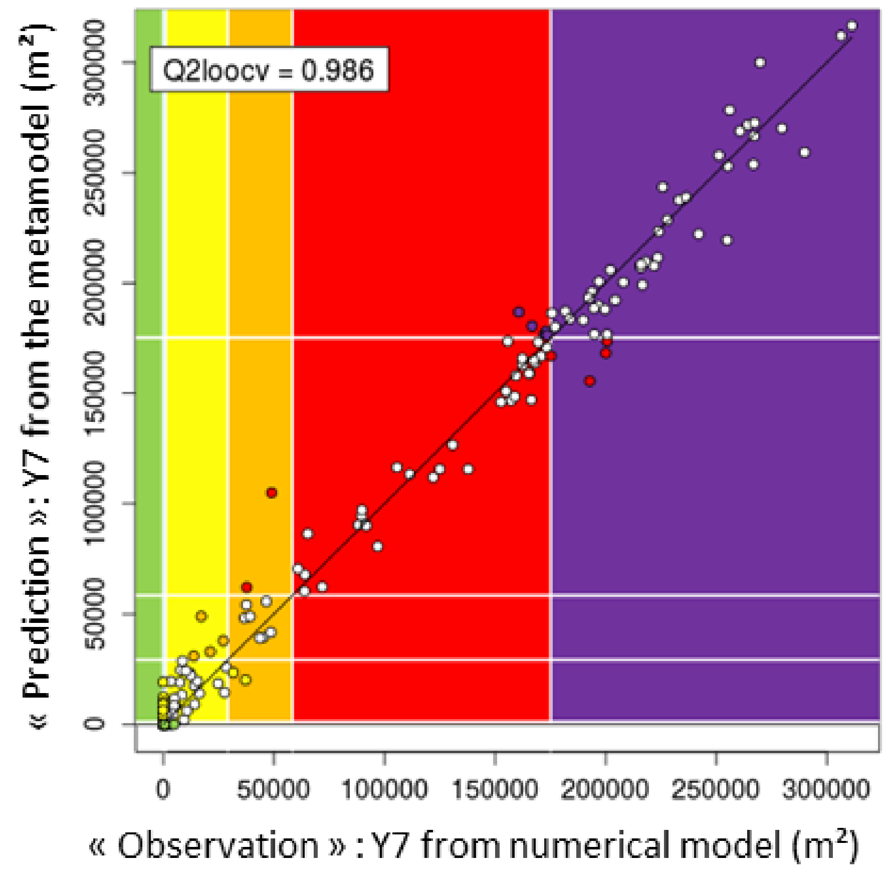
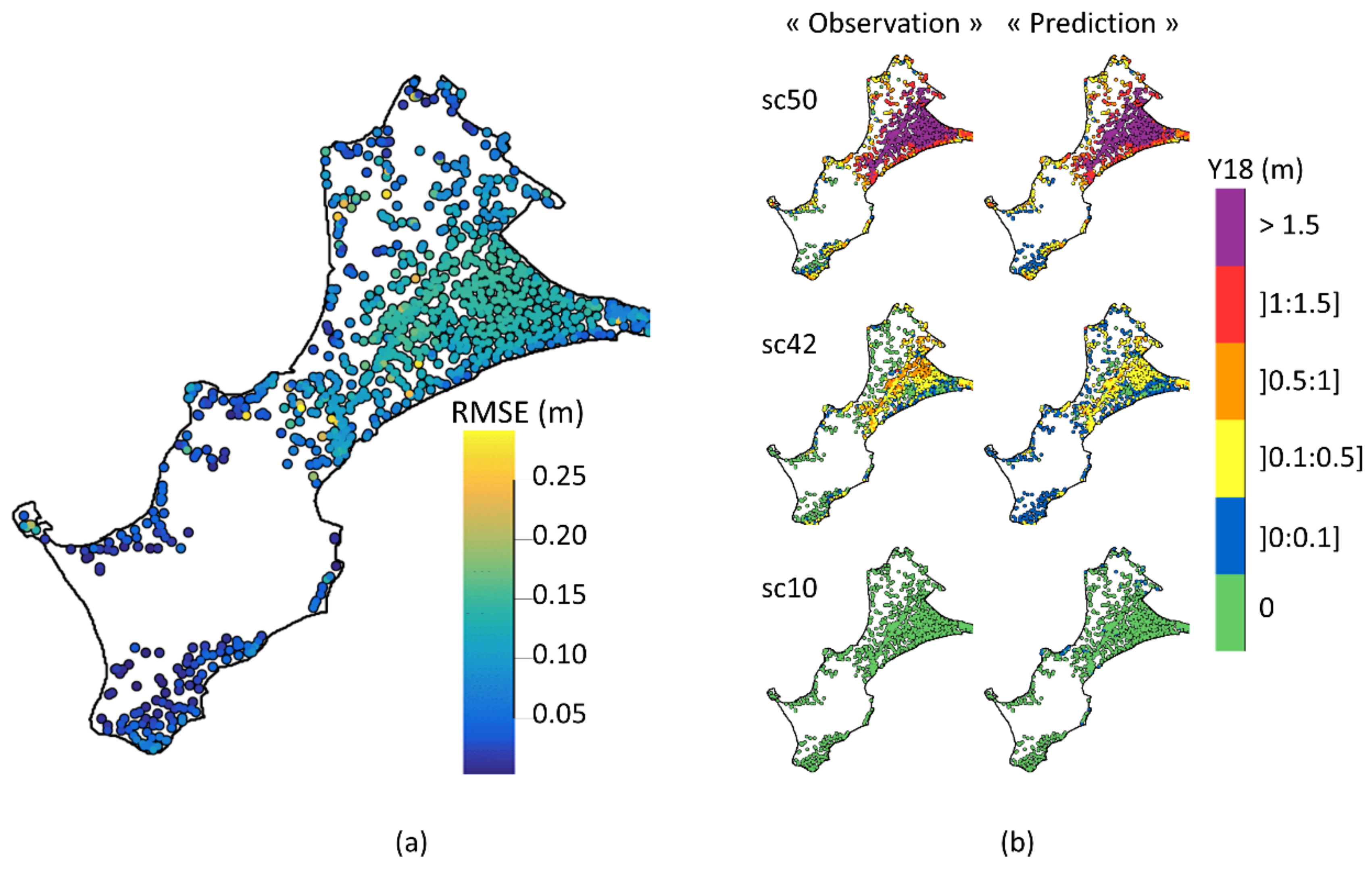
3.2. Metamodel Cross-Validation

The predictive capabilities of the different metamodels are assessed by applying the cross-validation procedure [40].
For the metamodels with scalar inputs (Y1 to Y6), the widely used 10-fold cross-validation method is performed (see [40]). Figure 9 provides a comparison between the observations (the numerically calculated Ynum values) and the predictions of the GP-based metamodels; their agreement reflects a highly satisfactory prediction quality. This consistency is further confirmed by the high coefficient of determination Q2 calculated using the residuals derived from the cross-validation procedure. The closer Q2 is to one, the more satisfactory the capability of the GP-based metamodel to predict the considered Y. In our case, Q2 is not lower than 95%, and hence, it is considered satisfactory. The predictive capability of the RF model for Y1 is measured by the accuracy of the classification (denoted ACC), which is defined as the ratio of the number of events correctly classified by the RF model to the total number of events. In our case, ACC reaches 92%, which can be considered satisfactory.
The functional input, scalar output metamodels (for the prediction of Y7Y17), are validated using a leave-one-out (LOO) cross-validation procedure. Here, using LOO cross-validation enables us to benefit from explicit virtual LOO formulas (Bachoc et al., 2013; Zhang and Wang, 2010). Figure 10 illustrates the performance of the metamodels on the prediction of the maximal flooded surface (Y7). The metamodelling quality is assessed by comparing the LOO predictions with the values obtained by the numerical model. As in the case of the scalar input metamodels, the results show a satisfactory prediction quality, which is further supported by a fairly high Q2 value. In addition, the class is correctly predicted for the vast majority of the points (white dots). However, at this stage, we note that Y7num values equal to 0 are overestimated. Appendix B presents the validation plots for the metamodels for the prediction of Y8 to Y17.
To assess the predictability of the spatial GP-based model, we again perform LOO cross-validation where each flood scenario from the dataset is predicted using data from the other scenarios. First, we compute the root mean square error (RMSE) for the 1003 designed points, i.e., the RMSE over the 174 LOO predictions. For the purposes of our FEWS, we remove the points for which the RMSE is larger than 0.3 m, leading to the removal of 14 points from the 1003 initial points. Figure 11 shows the RMSE values obtained for the remaining 989 points. Using the colour scale in Figure 3, Figure 11b shows the predictions for scenarios 50, 42, and 10. The model globally captures the category of those scenarios. One must note that a misclassification between consecutive flood categories (e.g., between the green and blue categories) results mainly from overestimation or underestimation around the given threshold that defines the limit between the two categories. Appendix C shows additional figures regarding the cross-validation for learning scenarios 50, 42, and 10 together with their confidence intervals, revealing non-negligible confidence intervals (e.g., ±40 cm) in comparison with the water height classes (Figure 3).

3.3. Indicator Predictions: Raw Results, Optimisation, Hindcast, and Reinforced Hindcast

To estimate the quality of the metamodel predictions, we consider the period 1900–2010. From the analysis of historical information, five major flooding events occurred during this period, while another four events led to a sparse number of overtopping phenomena [7]. We do not have knowledge of the historical values of each indicator, but we do know whether each scenario was a non-flood, minor flooding (few instances of overtopping, equivalent of the class-2 intensity indicator), or major flooding event. We also attribute a confidence index to each event within the damage event database [7]. Indeed, for some of the damage events, it is not possible to be fully certain that either there was no flood or there were few instances of wave overtopping. In addition, it is important to note that the territory of Gâvres is now more protected from floods than it was during 1900–2010. This implies that the predicted indicators following our method can be considered satisfactory if they fulfil the following conditions: (1) if the historical database indicates no submersion, then the prediction should be a non-flood event; (2) if the historical database indicates minor flooding, then the prediction should provide either a minor flooding or a non-flood event; and (3) if the historical database indicates major flooding, then the prediction should provide at least a minor flooding event.
Our main calibration parameter is V1 (threshold of the water volume entering inland in 15 min; see Section 2.6). Thus, we optimise the V1 values to minimise (maximise) the number of false (true) alarms over the 48 events within the damage events database. Figure 12 shows the Z1 predictions over the continuous forcing conditions from 1900 to 2010 and the 48 damage events, together with the optimisation curve of V1, leading to V1 = 62 m3. With this value, considering that 0 < Z1 < V1 leads to a simple warning and Z1 ≥ V1 leads to a real flood alarm, we obtain four true flood event alarms and two false alarms. Over the entire 110-year period, this threshold leads to the prediction of only nine flood events and 102 “warning” events, implying that for DEM2015–2018, there is an empirical probability of 1 “warning” (few instances of overtopping) per year and 1 “alarm” per decade. Regarding the two false alarms (1948 and 1957), it should be noted that for both events, the confidence level of the classification between no flooding and minor flooding is moderate [7] such that it is possible that minor flooding did not occur on either date. The 1904 event is classified with moderate confidence as a major flood from an analysis of the historical information [7] such that this event may have been a minor flood instead of a major flood, but we are sure that there was a flood. Thus, the number of false alarms (i.e., two) should be considered as the upper limit of the real number of false alarms. Finally, two events are not clearly identified in the damage event database: those on 18 December 1945 and 19 December 1945. However, after [60], strong erosive events may have occurred in December 1945. Focusing on the four remaining flood events of the damage database, (1) consistent with our validation assumption, Z1 = 0 for two past minor flooding events and 0 < Z1 < V1 for one past major flooding event (considering the less protective topo-bathymetry during the studied period), and (2) Z1 = 0 for the past major flooding event on 10 January 2001. The result for this last event is not inconsistent. Indeed, in comparison to the other major flooding events, the water level, wave, and wind conditions are not exceptional (with a joint exceedance return period of the water level and significant wave height of less than 1 year); in fact, this event was caused by a coastal defence failure, which led to significant flooding [7]. The failure of coastal defences is not accounted for in our method/FEWS (see Section 4.1 for a more detailed discussion).
Applying the optimised value V1 = 62 m3 and the constraint scheme shown in Figure 5, we obtain predictions for all the indicators Ij over the period 1900–2010. Figure 13 shows the results only for the events where Z1 > 0 (i.e., the intensity indicator I1 falling in a class larger or equal to 2) or Z1 > V1 (i.e., such that C(I1) ≥ 3) for the sake of readability. First, we note the consistency of the predictions between the indicators: only minor flooding events are predicted, while neither the roads nor the crisis management buildings are flooded (I9 to I13). The predictions indicate that the riskiest survey points are GP4 (I5) and G1 (I6). This is consistent with Figure 8 and with local knowledge, which indicates that the preferential pathway of flooding is in front of the cemetery (i.e., GP4). Furthermore, significant human risk (C(I5) and C(I6) reaching up to 4, in red) is predicted for these survey clusters (corresponding to I5 and I6), while the intensity (I1) is small (C(I1) = 2 most of the time, in blue). This can physically be explained by the fact that both survey clusters are located in areas more subject to wave overtopping, i.e., locations where individual waves overtop the defences. Due to the stochastic behaviour of waves, in the (HT − 3 h:HT + 3 h) time window, only a single wave (or a few waves) may overtop the defences, leading to a local instantaneous water depth of a few tens of centimetres (i.e., C(I5) or C(I6) = 3 (0.1 to 0.25 m, in orange) or 4 (0.25 to 0.5 m, in red)), but they may move only a limited volume of water onto land (e.g., <V1, with V1 = 62 m3); consequently, the flood intensity remains small (C(I1) = 2, blue class, Figure 3).
To compare the skills of the more inland indicators (I1, I7 through I13), numerical simulations are performed for the nine events where the predicted class of indicator I1 is larger than or equal to 3 (Figure 14). The comparison with the predicted values (Figure 13) shows that our predictions are relatively coherent with the “truth” (here, the direct numerical results Ynum), even for these “on the edge” events, i.e., events that are difficult to properly predict with metamodels. For this hindcast, there are no cases where the intensity I1 is large enough to fulfil the visualisation conditions of the I14 indicator.
However, we note that we would produce many more predicted flood events using a less protective bathymetry. The methods used to construct the scalar input metamodels have previously been used with a smaller learning dataset and with numerical modelling relying on a topo-bathymetry representative of 2008 (i.e., DEM2008, less protective). These metamodels exhibit good prediction skills compared to the historical flood events over 1900–2016 and yield much larger predicted quantities than those obtained with the (more protective) 2015–2018 topo-bathymetry.

3.4. FEWS: Operational Use of the FEWS and First Feedbacks

Appendix D provides screen captures of the FEWS web interface, which allows the visualisation of all the indicators for the next six high tides, except indicators I7, I8, and I14, which are provided only when a flood event (alarm) is predicted (C(I1) ≥ 3). In addition, for I14, the cross-validation reveals a non-negligible confidence interval (e.g., ±40 cm, Figure A4 in Appendix C); in comparison with the water height classes (Figure 3), we stipulate that the I14 predictions are of low confidence. Access to the FEWS interface was provided to the local users in December 2020. According to the users’ first feedback, they found it very easy to use and to understand.
Even though access to the FEWS was given to the local users in December 2020, the FEWS existed (i.e., was in development) beforehand, as forecasted forcing data were downloaded since September 2019. This allows us to evaluate the prediction quality from September 2019 until March 2021 (Table 3). During this period, the town hall did not report any flooding in the study area. It may happen that the events with only a few wave overtopping episodes were not observed (as overtopping is a highly local phenomenon in time and space), which implies that during the study period, the maximum value of C(I1) should be 2. Over the study period, the FEWS predicts C(I1) = 1 most of the time. Table 3 lists all the events for which either the FEWS predicted C(I1) > 1 or an official VVS warning was issued by Meteo-France at the department scale. With XMARC (XDATASHOM), the FEWS predicts eight (1) events “close to flood” (C(I1) = 2); i.e., the FEWS issued only warnings but no alarms for flooding events. Such predictions (i.e., usually C(I1) = 1, a few cases with C(I1) = 2, and no cases where C(I1) > 2) are in fair agreement with the information provided by the town hall. To complement the town hall information, photos were gathered on the internet. For the events for which we found photos (Table 3), they allowed the identification of high water levels in the study area and a few instances of overtopping events either within or near the study area. These photos confirm the good agreement between the predictions and observations. The only “discrepancy” is discovered for the last event (30 January 2021), where few instances of overtopping were captured in a photograph, while the FEWS predicts C(I1) = 1. As the numerical modelling with the XMARC input provides C(I1) = 2, this finding implies that improved metamodels for such types of events could lead to C(I1) = 2.
Regarding the sensitivity to the time horizon (1, 2, or 3 days), the FEWS predictions are not very sensitive (the prediction of I1 performed 3 days in advance is, for most events, equal to that performed 1 day in advance); consequently, we can trust the predictions obtained 3 days in advance for the validation period. Table 3 also includes the VVS warnings over the study period. The FEWS issues more warnings than the VVS, albeit with a lower level (blue level, “close to flood” events) than those issued by the VVS (orange level). The VVS has four warning levels (in increasing severity: green, yellow, orange, red). The recommendation associated with the orange level is that dangerous phenomena are expected and that the population should be very vigilant, stay up to date with developments, and follow the safety advice issued by authorities. Thus, our FEWS predictions seem closer to what happens locally (either nothing or only a few instances of overtopping), at least over the investigated time span from September 2019 to March 2021.
Finally, it should be noted that in the FEWS version provided to the local users, by default, the XMARC data are used; if these data are not available, the XDATASHOM (which are always available) are used. This allows a small security margin to be adopted but still limits the number of false alarms (as highlighted in the validation for the period 2019–2021 where the FEWS, even with the XMARC data, provided no alarms and only a few blue warnings).

4. Discussion and Recommendations

4.1. Discussion

The FEWS prototype exhibits good prediction skills and relies on a simple interface satisfying the local users. However, we report two main issues.
First, regarding the prediction skills of the metamodels, to address the lower skills of the GP-based metamodels (Y7:18) close to 0, we adopt a pragmatic approach of using the classification metamodel (Y1) outputs and combining them with the GP-based metamodel outputs. However, from a theoretical point of view, this is not fully satisfactory. One way to improve the indicators relying on the GP-based metamodels close to 0 is to increase the number of learning scenarios providing Y = 0 values. We tested this strategy by adding 40 non-flood event scenarios to the existing 174 scenarios used in the learning dataset; no significant improvement was found. A more promising perspective of improvement is to use refinements of GP models that are tailored for modelling positive functions and may provide more accurate metamodel predictions of output values close to zero. Two main examples of these refinements are truncated GP models [57] and constrained GP models [61,62]. If metamodels other than GPs are considered, then it would also be possible to have an interaction between the classification problem of zero outputs and the regression problem of non-zero outputs. Possibilities that would warrant investigation are to tailor the loss function for metamodels relying on empirical risk minimisation (see [40]) or to use nearest-neighbour methods. In the latter case, the rationale is that the averages of the observed outputs are non-negative and are exactly zero when all outputs are zero.
Building such an FEWS requires considerable amounts of human and computational effort (thousands of hours of computation). The FEWS discussed herein was built for a given topo-bathymetry (DEM). If the beach morphology changes or coastal defences are modified (or damaged, as was the case during the 10 January 2001 flood event), then the prediction skills of the FEWS are expected to decrease. In the case of significant changes, we may need to redo all the steps (numerical modelling, metamodelling, validation of metamodel outputs and indicators, and update) to re-establish the FEWS. A more flexible approach would be to add one level of complexity to the metamodels by allowing them to account for the topo-bathymetry as spatial (functional) inputs of the metamodels themselves. This would require methodological and mathematical developments together with the optimisation of the numerical computation. Relevant starting points for adding the topo-bathymetry as an input to the GP-based metamodels are the developments of [52,63], which address functional inputs and positive map inputs, respectively. Other promising approaches have also been investigated, such as stochastic partial differential equations combined with integrated nested Laplace approximation, as described by [64], for handling complex spatially varying inputs for tsunamis.
In this paper, by combining historical data, extreme value analysis, advanced numerical modelling, metamodelling, and pragmatic post-processing, we show how it is possible to predict coastal flood information (including the prediction of inland flooding) with fair quality and negligible computation times (typically within 1 min for one scenario). This methodology may have several potential implications in flood management and/or decision processes that are not limited to the improvement of FEWSs and to raising awareness. For instance, the rapid models developed in our approach may be able to directly contribute to the real estimation of coastal risks; in theory, the risk estimate should be based on a fully probabilistic analysis in which all possible scenarios and their consequences are included [65] and not on a limited number of scenarios. This approach also provides fresh perspective with regard to preparing for climate change and sea-level rise. For instance, the metamodel providing the water volumes entering inland may be used to estimate the present-day and future probabilities of exceedance while accounting for uncertainties in future sea-level rise and thus to identify when (at the earliest and latest) tipping points may be reached [66]. Finally, our methodology may be of indirect use for the design of coastal defences (structural measures to reduce flood risks). Indeed, additional developments in metamodelling techniques to allow treating the DEM as an input variable (see the discussion above) would allow us to investigate a large number of coastal defence configurations, estimate the associated flood risks, and define the most acceptable coastal defence plan that minimises the risk (see [67] for an example of optimising floodgate operations for river flood management).
Model-based FEWSs may also benefit from citizen science. Within the CoastSnap global citizen science project, which aims to capture changing coastlines [68], a station was recently installed at the Gâvres site. Even if this station was not designed for coastal flood purposes, it still captures the coastal defences in front of the cemetery (the preferential water pathway) and thus may provide very valuable information in terms of validating our coastal FEWS. From a broader perspective, citizen science (e.g., through crowdsourced observations, [69]) can deliver a level of spatial granularity often not possible with conventional research [70] such that it is also used in crisis management (see, e.g., [71,72]). As an example, the Virtual Operations Support Team (VOST or VISOV for the French speaking part) inspired by the American model of utilising social media in emergency management helps operational emergency organisations by collecting information on social networks and by quickly providing analysed and verified information from the field. During crises, such crowdsourced information may be of use, for instance, to better qualify forecasted data.

4.2. Recommendations

The presented method, which has been developed and tested at the Gâvres study site, presents real potential for many other locales subject to marine flooding. However, the proposed method requires both on-site knowledge and numerical modelling methods that need to be adapted to each considered site. Indeed, the choice of the model used depends on the size of the site and on the flooding process. For the FEWS prototype at Gâvres, the SWASH model was chosen to precisely model the wave overtopping processes and the resulting flood. The entire modelling chain (WW3-SWASH) requires a significant computation time (3 days to model 6 h on 48 cores, with SWASH representing 97% of the computation), so the use of metamodelling is a relevant solution to tackle the excessive computation time. However, this may not always be the case depending on the site dimensions and characteristics. For instance, if a particular site is not affected by wave overtopping, other process-based models instead of a phase-resolving model such as SWASH may be chosen to compute the flood by relying, for instance, on mass conservation schemes (e.g., LISFLOOD-FP, [73]) and simple inertial formulations of the shallow-water equations (e.g., [74]); other alternatives include hydrodynamic models such as TELEMAC2D or MIKE FLOOD, which solve the full 2D shallow-water equations. Such models have much smaller computation times, and thus, their use may be fully compatible with requirements of FEWSs; in this case, then, there would be no need to implement metamodelling techniques. To adapt the proposed methodology to a new site, local knowledge also needs to be acquired, including the identification of past flood events at the site and their forcing hydro-meteorological conditions. Recent efforts to build historical flood databases at national scales (see, e.g., [75,76]) may support this work. In addition, users’ needs and the selected targets have to be defined together with local stakeholders even if there are similarities with the Gâvres site.
Once a model is chosen according to the previously mentioned parameters (the site dimensions and flooding processes), the model can be fed the DEM of the area (including the coastal defences) and validated on at least one reference flooding event. A key issue is the availability of sufficiently precise topo-bathymetric data; moreover, especially if significant coastal changes have recently occurred, these data should be relatively fresh. At least for the topography, the vertical precision should be on the order of a few centimetres, especially if high local prediction skills are to be expected. Such precision can be reached, for instance, by using lidar technologies or performing differential GPS (DGPS) surveys. Then, the numerical model can be set up and validated, preferably via comparisons with past flood events.
If the computation time of the hydrodynamic model chain is too long for forecast purposes, then a metamodel should be established. To construct the metamodel, the maximum number of possible numerical simulations should be estimated regarding the available computational resources. As a recommendation, rather than directly defining all the scenarios X, we advise designing the scenarios in a stepwise (iterative) fashion: define the first set of scenarios (smaller than the maximum number of possible simulations), analyse the numerical results, set up the metamodels, and validate; then, identify the X domain of lower skills and define a new set of scenarios, perform the complementary numerical simulations, and rebuild the metamodel. This step could benefit from advances in the sequential design of computer experiments (e.g., [77]). Using the resulting metamodels, the metamodel must be validated once again against the numerical model; in addition, the historical and contemporary events must be compared (i.e., to truly assess the FEWS output quality). Depending on the metamodel skills, the pragmatic approach we used for Gâvres of combining the metamodels (Figure 5) may be of use to compute the final indicators of interest for the site.
Thus, the adaptation of the method we applied at Gâvres to construct the FEWS prototype would require skills in history, statistics, modelling, computing, and decision making and would require both a significant number of staff members and considerable computational efforts depending on the existing knowledge, data, and local flood processes.

5. Conclusions

In the present work, we establish an FEWS prototype to predict local coastal flooding using the metamodelling approach to tackle the excessive computation time required by numerical models. We show that both numerical models and metamodels are sufficiently mature to provide fresh perspectives for forecasting local coastal flooding, even in locations where wave overtopping is the main flood driver. The pragmatic approach of correcting the metamodel outputs allows the weaknesses of some of the metamodels (mainly those with functional inputs) to be overcome. Even if metamodel developments are still needed, we demonstrate that metamodelling techniques (some being available in the literature and others specifically dedicated to handling functional inputs/outputs) can be employed to forecast coastal floods at local complex sites given that the predictions are carefully validated. One of the key future challenges is probably to develop metamodelling techniques that allow the topo-bathymetry to be treated as an input variable while maintaining good prediction skills. This would drastically ease the requirement for the users to update the FEWS themselves.

Author Contributions

Conceptualisation, A.A., D.I., F.G., J.R.; Methodology, A.A., A.F.L.-L., D.I., F.B., J.B., J.R., F.G., R.P., T.K.; Software, A.F.L.-L., A.T., D.I., J.B., J.R., R.P.; Validation, A.F.L.-L., A.T., D.I., J.B., J.R.; Data Curation, A.T., D.I.; Writing—original draft, A.B., A.F.L.-L., D.I., F.B., J.B., J.R.; Writing—review and editing, D.I., F.B., J.R.; Visualisation, A.A., A.F.L.-L., D.I., F.B., J.B., J.R.; Supervision, D.I.; Project administration, A.A., D.I., F.G.; Funding acquisition, A.A., D.I., F.G. All authors have read and agreed to the published version of the manuscript.

Funding

This research was funded by Agence National de la Recherche (ANR) grant ANR-16-CE04-0011 (RISCOPE project), BRGM, Antea Group and IMT.

Data Availability Statement

The data produced in this study are available on request from the corresponding author, at the exception of data provided by a 3rd party.

Acknowledgments

The following data providers are acknowledged: LEGOS, NOAA, LOPS-IF REMER, SHOM, and Météo-France. The authors are also grateful to the Lorient Agglomeration for providing lidar survey data, to D. Paradis for providing VVS information, to S. Le Roy for his participation to the user’s workshops, to G. Le Cozannet for his contribution to the revision of the present manuscript, and to the user committee and advisory committee members of the RISCOPE project. Finally, the reviewers thank the two reviewers of this manuscript for their constructive comments.

Conflicts of Interest

The authors declare no conflict of interest. The funders had no role in the design of the study; in the collection, analyses, or interpretation of the data; in the writing of the manuscript; or in the decision to publish the results.

Acronyms and Abbreviations

ACO-GpAnt colony-based algorithm for the structural optimisation of Gaussian process models with scalar and/or functional inputs
CRANComprehensive R Archive Network
DDTM56Direction Départementale des Territoires et de la Mer (translation: Departmental Directorate of Territories and the Sea) of French department 56 (Morbihan)
DEMDigital elevation model
DGPSDifferential Global Positioning System
DHIDanish Hydraulic Institute
FEWSForecast and early warning system
GPGaussian process
HTHigh tide
HPCHigh-performance computing
IGNInstitut National de l’Information Géographique et Forestière (translation: National Institute of Geographic and Forestry Information)
LOOLeave one out
LOPSLaboratoire d’Océanographie Physique et Spatiale (translation: Physical and Space Oceanography Laboratory)
MARCModélisation et Analyse pour la Recherche Côtière (translation: Modelling and Analysis for Coastal Research)
MEDDTLMinistère de l’Écologie, du Développement Durable des Transports et du Logement (translation: Ministry of Ecology, Sustainable Development, Transport and Housing)
MIKE21software package for the 2D modelling of hydrodynamics, waves, sediment dynamics, water quality and ecology; for more details, see https://www.mikepoweredbydhi.com/products/mike-21-3, accessed on 25 July 2021
PCAPrincipal component analysis
RFRandom forest
RGERéférentiel à grande echelle (translation: large-scale reference system)
TELEMAC2Dmodule of the TELEMAC system for solving the Saint-Venant equations using The finite-element or finite-volume method and a computational mesh of triangular elements; for more details, see http://www.opentelemac.org, accessed on 25 July 2021
SDIS56Service Départemental d’Incendie et de Secours (translation: Departmental Fire and Rescue Service) of French department 56 (Morbihan)
SHOMService Hydrographique et Océanographique de la Marine (translation: French Navy Hydrographic and Oceanographic Service)
SWASHSimulating Waves till Shore. SWASH is a general-purpose numerical tool for simulating unsteady, non-hydrostatic, free-surface, rotational flow and transport phenomena in coastal waters driven by waves, tides, buoyancy and wind forces. It provides a general basis for describing wave transformations from deep water to a beach, port, or harbour, complex changes to rapidly varied flows, and density-driven flows in coastal seas, estuaries, lakes and rivers. For more details, see https://swash.sourceforge.io/, accessed on 25 July 2021
VISOVVolontaires Internationaux et Soutien Opérationnel Virtuel (translation: International Volunteers and Virtual Operational Support)
VOSTVirtual Operations Support Team
VVSVigilance Vague Submersion (translation: wave-flood warning)
WW3WAVEWATCH III®, a community wave modelling framework that includes the latest scientific advancements in the field of wind-wave modelling and dynamics

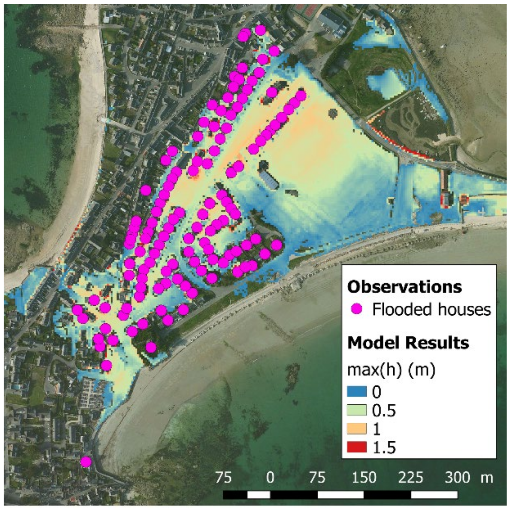
Appendix A. The Flood Event on 10 March 2008 (Observations and Model Results)

To validate the modelling chain for the 10 March 2008 flood event, the chain was run for 6 h centred on the high tide using the following forcing conditions: the still water level modelled in Le Roy et al. (2015), the wave conditions coming from Norgasug [78], and the wind extracted from the Climate Forecast System Reanalysis (CFSR) hindcast [79]. For the time series of forcing conditions, see [6].
Figure A1. Model validation: maximal simulated water depth and observed flooded houses during the Johanna event. Source: [6].
Jmse 09 01191 g0a1

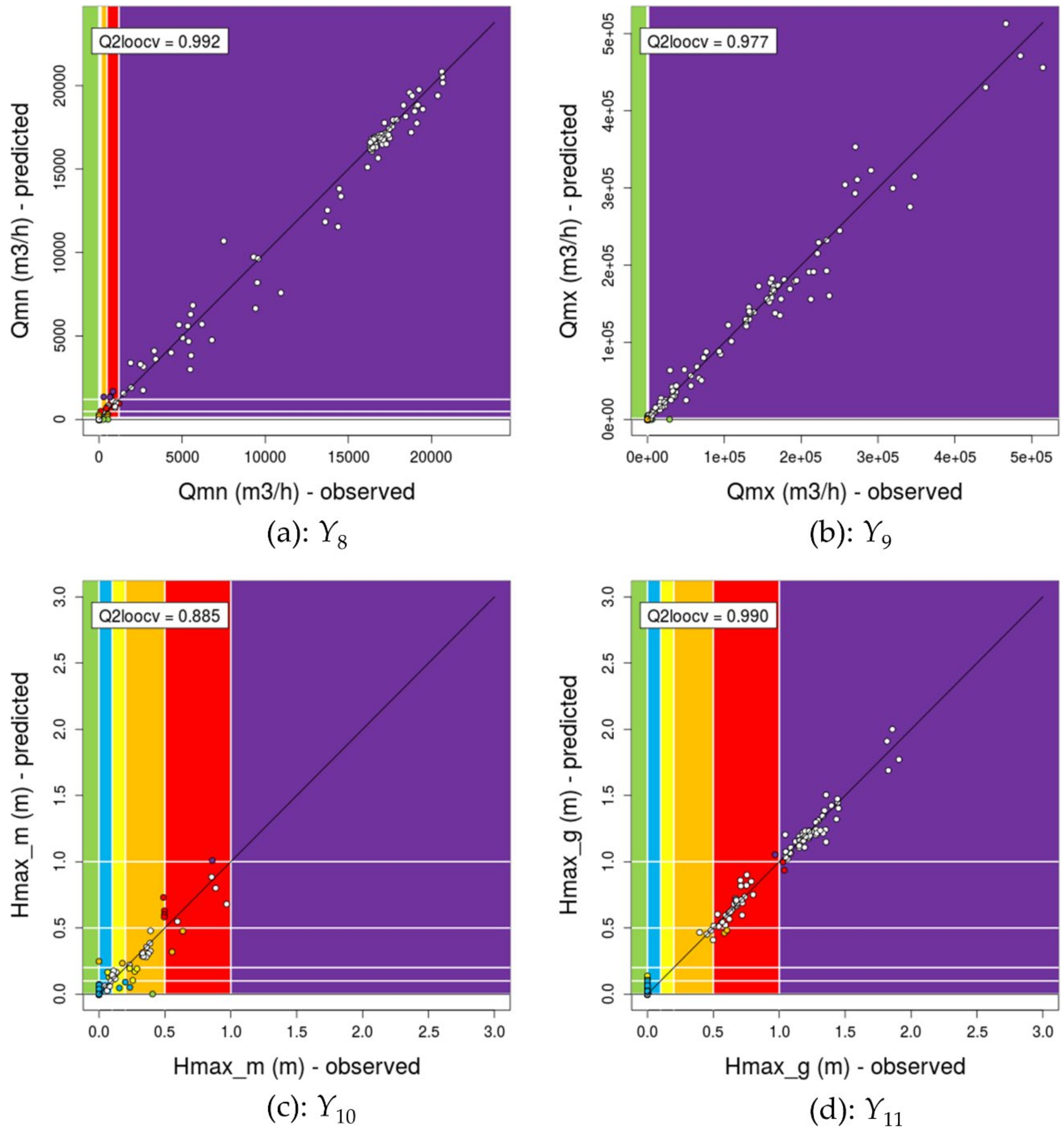
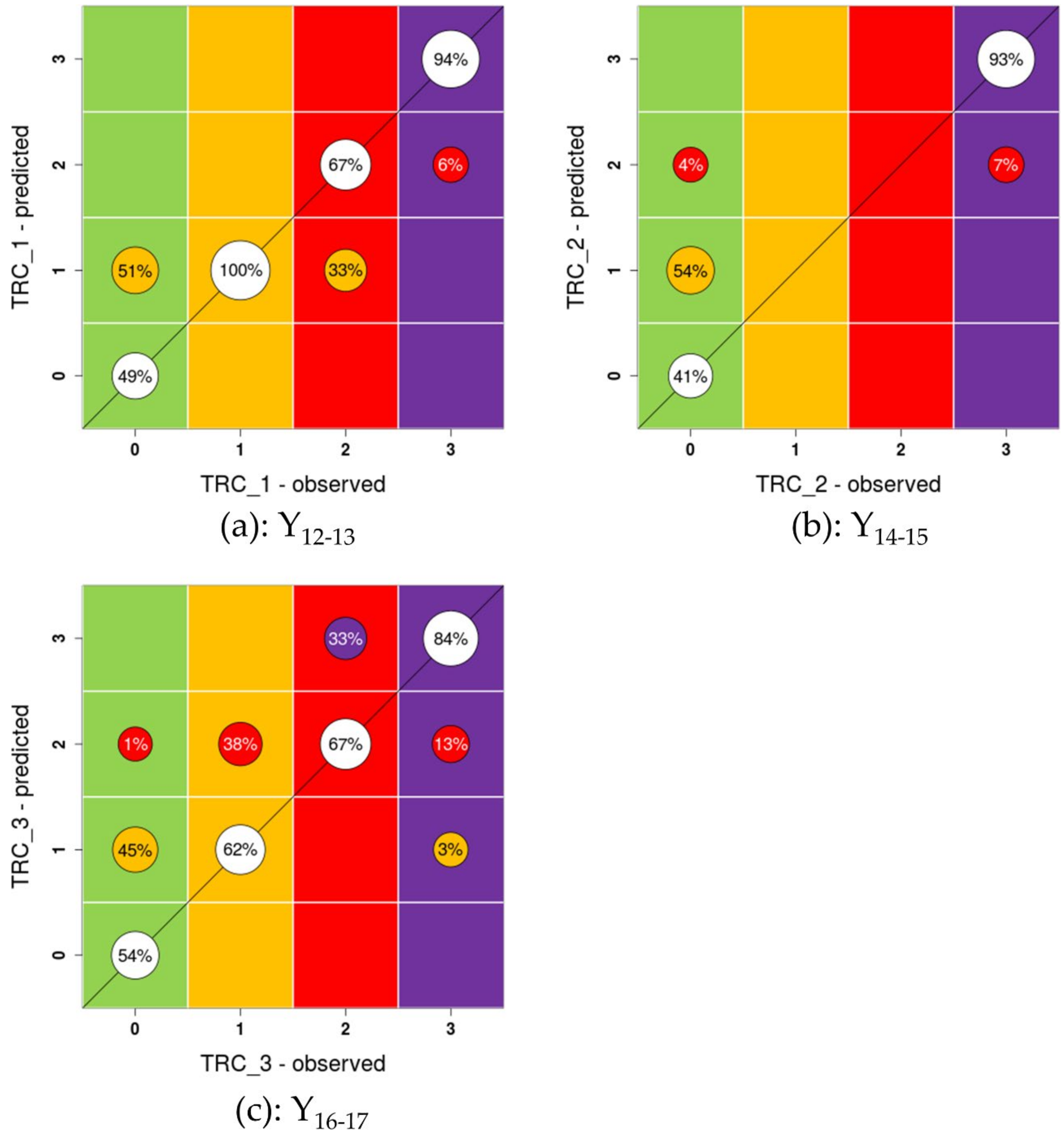
Appendix B. Cross-Validation Plots for Metamodels Y8 to Y13

This appendix is a complement for Figure 10, showing the validation plots for the remaining functional input, scalar output metamodels. Note that panels (d) to (f) present confusion plots instead of regular calibration plots since these plots correspond to the categorical trafficability of the three main roads. For each observed class (i.e., each column of the figure), we provide both the percentage of points correctly classified and the percentage of those classified in wrong classes. The overall performance of each metamodel is satisfactory, with high Q2 values for the continuous outputs and a high percentage of hits for the categorical outputs.
Figure A2. Cross-validation of the Y8–Y11 metamodels: comparison between the observations (the numerically calculated Y values) and the predictions of the GP-based metamodels. The colour scales correspond to the colour scales of the indicators using these metamodels (see Figure 3 and Table 1).
Jmse 09 01191 g0a2
Figure A3. Cross-validation of the Y12–Y17 metamodels: comparison between the observations (the numerically calculated Y values) and the predictions of the GP-based metamodels. The colour scales correspond to the colour scales of the indicators using these metamodels (see Figure 3 and Table 1).
Jmse 09 01191 g0a3

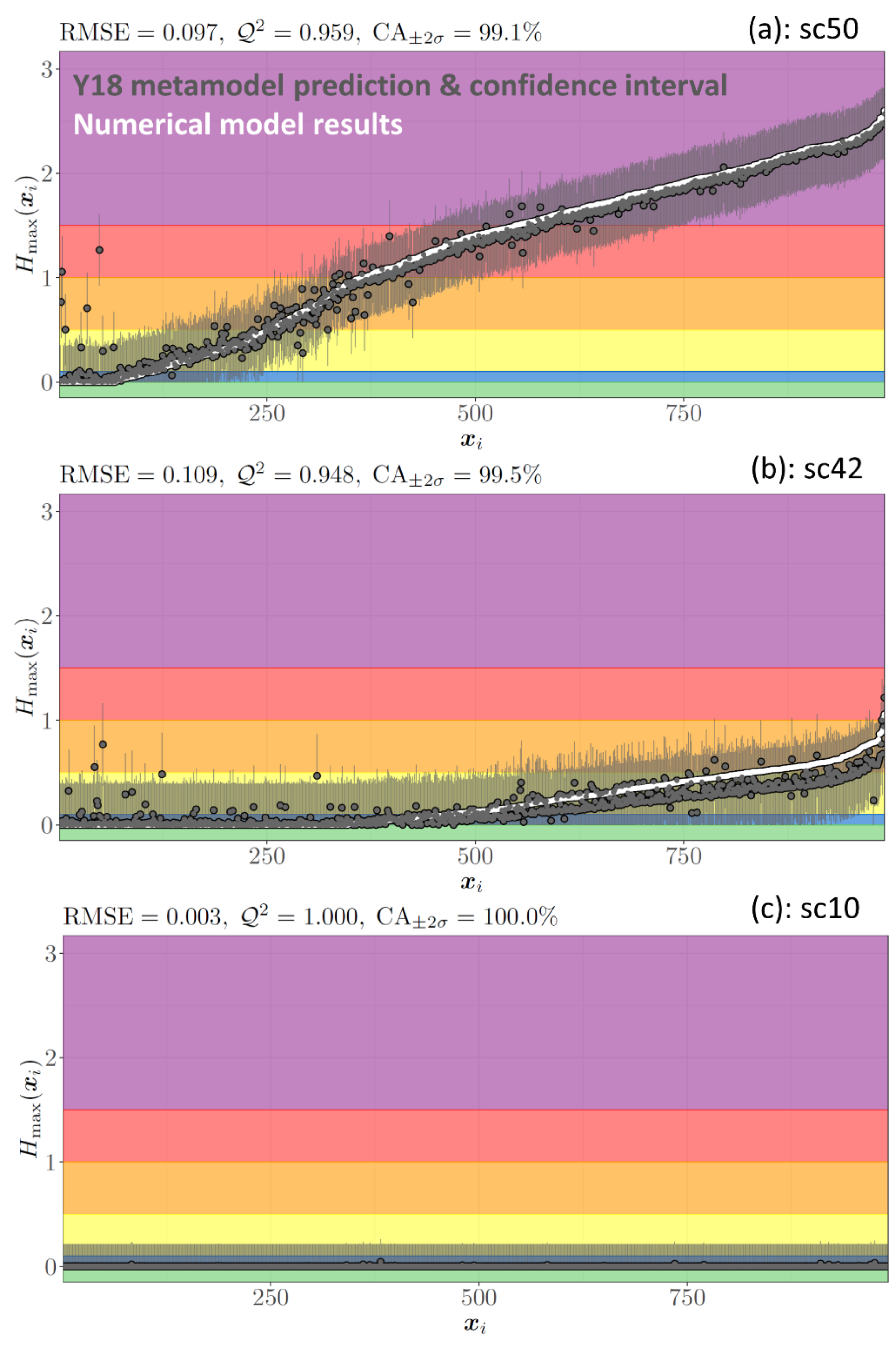
Appendix C. Cross-Validation Plots for Metamodel YI8

This appendix completes Figure 11 regarding the cross-validation for learning flood scenarios 50, 42, and 10. The figure shows the predicted and observed values of the (maximal) water height level at the 889 spatial design points used in Figure 10 together with two standard-deviation confidence intervals.
Figure A4. Cross-validation of the maximal water heights predicted by metamodel Y18 and provided by the numerical model for scenarios 50, 42, and 10 among the 174 learning scenarios. Xi is the index of the spatial points (from 1 to 889, sorted in increasing order using the numerical results for each scenario). The panels show the RMSE, Q2, and CA (coverage accuracy) indicators. The CA indicator quantifies how many test points are contained in the two standard-deviation (denoted σ) confidence interval.
Jmse 09 01191 g0a4

Appendix D. Screen Captures of the FEWS User Interface

Figure A5. Screen capture of the FEWS webpage synthesising predictions for the six next high tides. The left panel shows the results of the I1 indicator (shown in green here, as no flood is predicted).
Jmse 09 01191 g0a5
Figure A6. Screen capture of the FEWS webpage showing indicators I1 to I6 and I9 to I13. The other indicators are shown only when C(I1) > 2, which is not the case for the present prediction.
Jmse 09 01191 g0a6
Figure A7. Screen capture of the FEWS webpage showing the forcing conditions X (here, X = XMARC). The forcing conditions in orange correspond to the last major flooding event (10 March 2008, Windstorm Johanna).
Jmse 09 01191 g0a7

References

  1. McGranahan, G.; Balk, D.; Anderson, B. The rising tide: Assessing the risks of climate change and human settlements in low elevation coastal zones. Environ. Urban. 2007, 19, 17–37. [Google Scholar] [CrossRef]
  2. Oppenheimer, M.; Glavovic, B.C.; Hinkel, J.; van de Wal, R.; Magnan, A.K.; Abd-Elgawad, A.; Cai, R.; Cifuentes-Jara, M.; DeConto, R.M.; Ghosh, T.; et al. Sea Level Rise and Implications for Low-Lying Islands, Coasts and Communities. In IPCC Special Report on the Ocean and Cryosphere in a Changing Climate; Pörtner, H.-O., Roberts, D.C., Masson-Delmotte, V., Zhai, P., Tignor, M., Poloczanska, E., Mintenbeck, K., Alegría, A., Nicolai, M., Okem, A., et al., Eds.; IPCC: Geneva, Switzerland, 2019. [Google Scholar]
  3. Jongman, B. Effective adaptation to rising flood risk. Nat. Commun. 2018, 9, 1–3. [Google Scholar] [CrossRef] [Green Version]
  4. Zijlema, M.; Stelling, G.; Smit, P. SWASH: An operational public domain code for simulating wave fields and rapidly varied flows in coastal waters. Coast Eng. 2011, 58, 992–1012. [Google Scholar] [CrossRef]
  5. Le Roy, S.; Pedreros, R.; André, C.; Paris, F.; Lecacheux, S.; Marche, F.; Vinchon, C. Coastal flooding of urban areas by overtopping: Dynamic modelling application to the Johanna storm (2008) in Gâvres (France). Nat. Hazards Earth Syst. Sci. 2015, 15, 2497–2510. [Google Scholar] [CrossRef] [Green Version]
  6. Idier, D.; Pedreros, R.; Rohmer, J.; Le Cozannet, G. The Effect of Stochasticity of Waves on Coastal Flood and Its Variations with Sea-level Rise. J. Mar. Sci. Eng. 2020, 8, 798. [Google Scholar] [CrossRef]
  7. Idier, D.; Rohmer, J.; Pedreros, R.; Le Roy, S.; Lambert, J.; Louisor, J.; Le Cozannet, G.; Le Cornec, E. Coastal flood: A composite method for past events characterisation providing insights in past, present and future hazards—joining historical, statistical and modelling approaches. Nat. Hazards 2020, 101, 465–501. [Google Scholar] [CrossRef] [Green Version]
  8. Doong, D.-J.; Chuang, L.Z.-H.; Wu, L.-C.; Fan, Y.-M.; Kao, C.C.; Wang, J.-H. Development of an operational coastal flooding early warning system. Nat. Hazards Earth Syst. Sci. 2012, 12, 379–390. [Google Scholar] [CrossRef]
  9. Tromble, E.; Kolar, R.; Dresback, K.; Hong, Y.; Vieux, B.; Luettich, R.; Gourley, J.; Kelleher, K.; Van Cooten, S. Aspects of Coupled Hydrologic-Hydrodynamic Modeling for Coastal Flood Inundation. In Proceedings of the Eleventh International Conference on Estuarine and Coastal Modeling, Seattle, WA, USA, 4–6 November 2009; pp. 724–743. [Google Scholar]
  10. Stansby, P.; Chini, N.; Apsley, D.; Borthwick, A.G.L.; Bricheno, L.M.; Horrillo-Caraballo, J.M.; McCabe, M.; Reeve, D.E.; Rogers, B.; Saulter, A.; et al. An integrated model system for coastal flood prediction with a case history for Walcott, UK, on 9 November 2007. J. Flood Risk Manag. 2013, 6, 229–252. [Google Scholar] [CrossRef] [Green Version]
  11. Stokes, K.; Poate, T.; Masselink, G.; King, E.; Saulter, A.; Ely, N. Forecasting coastal overtopping at engineered and naturally defended coastlines. Coast. Eng. 2020, 164, 103827. [Google Scholar] [CrossRef]
  12. Merrifield, M.A.; Johnson, M.; Guza, R.T.; Fiedler, J.W.; Young, A.P.; Henderson, C.S.; Lange, A.M.Z.; O’Reilly, W.C.; Ludka, B.C.; Okihiro, M.; et al. An early warning system for wave-driven coastal flooding at Imperial Beach, CA. Nat. Hazards 2021, 108, 2591–2612. [Google Scholar] [CrossRef]
  13. Mosavi, A.; Ozturk, P.; Chau, K.-W. Flood Prediction Using Machine Learning Models: Literature Review. Water 2018, 10, 1536. [Google Scholar] [CrossRef] [Green Version]
  14. Fotovatikhah, F.; Herrera, M.; Shamshirband, S.; Chau, K.-W.; Ardabili, S.F.; Piran, J. Survey of computational intelligence as basis to big flood management: Challenges, research directions and future work. Eng. Appl. Comput. Fluid Mech. 2018, 12, 411–437. [Google Scholar] [CrossRef] [Green Version]
  15. Kaya, C.M.; Tayfur, G.; Gungor, O. Predicting flood plain inundation for natural channels having no upstream gauged stations. J. Water Clim. Chang. 2017, 10, 360–372. [Google Scholar] [CrossRef]
  16. Dong, S.; Yu, T.; Farahmand, H.; Mostafavi, A. A hybrid deep learning model for predictive flood warning and situation awareness using channel network sensors data. Comput. Civ. Infrastruct. Eng. 2020, 36, 402–420. [Google Scholar] [CrossRef]
  17. Dai, W.; Tang, Y.; Zhang, Z.; Cai, Z. Ensemble Learning Technology for Coastal Flood Forecasting in Internet-of-Things-Enabled Smart City. Int. J. Comput. Intell Syst 2021, 14, 166. [Google Scholar] [CrossRef]
  18. Rohmer, J.; Idier, D. A meta-modelling strategy to identify the critical offshore conditions for coastal flooding. Nat. Hazards Earth Syst. Sci. 2012, 12, 2943–2955. [Google Scholar] [CrossRef]
  19. Jia, G.; Taflanidis, A.A. Kriging metamodeling for approximation of high-dimensional wave and surge responses in real-time storm/hurricane risk assessment. Comput. Methods Appl. Mech. Eng. 2013, 261–262, 24–38. [Google Scholar] [CrossRef]
  20. Simpson, T.; Poplinski, J.; Koch, P.N.; Allen, J. Metamodels for Computer-based Engineering Design: Survey and recommendations. Eng. Comput. 2001, 17, 129–150. [Google Scholar] [CrossRef] [Green Version]
  21. Basher, R. Global early warning systems for natural hazards: Systematic and people centred. Philos. Trans. R. Soc. A: Math. Phys. Eng. Sci. 2006, 364, 2167–2182. [Google Scholar] [CrossRef]
  22. Rohmer, J.; Idier, D.; Pedreros, R. A nuanced quantile random forest approach for fast prediction of a stochastic marine flooding simulator applied to a macrotidal coastal site. Stoch. Environ. Res. Risk Assess. 2020, 34, 867–890. [Google Scholar] [CrossRef]
  23. Betancourt, J.; Bachoc, F.; Klein, T.; Idier, D.; Pedreros, R.; Rohmer, J. Gaussian process metamodeling of functional-input code for coastal flood hazard assessment. Reliab. Eng. Syst. Saf. 2020, 198, 106870. [Google Scholar] [CrossRef] [Green Version]
  24. López-Lopera, A.F.; Idier, D.; Rohmer, J.; Bachoc, F. Multioutput Gaussian processes with functional data: A study on coastal flood hazard assessment. arXiv. 2020. Available online: https://arxiv.org/abs/2007.14052 (accessed on 25 July 2021).
  25. Idier, D.; Aurouet, A.; Bachoc, F.; Baills, A.; Betancourt, J.; Durand, J.; Mouche, R.; Rohmer, J.; Gamboa, F.; Klein, T.; et al. Toward a User-Based, Robust and Fast Running Method for Coastal Flooding Forecast, Early Warning, and Risk Prevention. J. Coast. Res. 2020, 95, 1111–1116. [Google Scholar] [CrossRef]
  26. Cariolet, J.M. Inondation des Côtes Basses et Risques Associés en Bretagne: Vers une Redéfinition des Processus Hydrodynamiques Liés aux Conditions Météo-Océaniques et des Paramètres Morphosédimentaires. Océan, Atmosphère. Ph.D. Thesis, Université de Bretagne Occidentale, Brest, France, 2011. [Google Scholar]
  27. Pedreros, R.; Idier, D.; Le Roy, S.; David, A.; Schaeffer, C.; Durand, J.; Desmazes, F. Infragravity Waves in a Complex Macro-tidal Environment: High Frequency Hydrodynamic Measurements and Modelling. J. Coast. Res. 2020, 95, 1235–1239. [Google Scholar] [CrossRef]
  28. Haiden, T.; Janousek, M.; Vitart, F.; Ben-Bouallegue, Z.; Ferranti, L.; Prates, F. Evaluation of ECMWF Forecasts, Including the 2021 Upgrade. Available online: https://www.ecmwf.int/en/elibrary/20142-evaluation-ecmwf-forecasts-including-2021-upgrade (accessed on 8 October 2021).
  29. Kramer, M.; Terheiden, K.; Wieprecht, S. Safety criteria for the trafficability of inundated roads in urban floodings. Int. J. Disaster Risk Reduct. 2016, 17, 77–84. [Google Scholar] [CrossRef] [Green Version]
  30. Jonkman, S.; Penningrowsell, E.C. Human Instability in Flood Flows1. JAWRA J. Am. Water Resour. Assoc. 2008, 44, 1208–1218. [Google Scholar] [CrossRef]
  31. MEDDTL. Guide Méthodologique Plans de Prévention des Risques Littoraux, 2014. Available online: https://www.ecologie.gouv.fr/sites/default/files/Guide%20PPRL%20-%20version%20finale%20mai%202014.pdf (accessed on 25 July 2021).
  32. Gallien, T.W.; Kalligeris, N.; Delisle, M.-P.C.; Tang, B.-X.; Lucey, J.T.D.; Winters, M.A. Coastal Flood Modeling Challenges in Defended Urban Backshores. Geosciences 2018, 8, 450. [Google Scholar] [CrossRef] [Green Version]
  33. Van der Meer, J.W.; Allsop, N.W.H.; Bruce, T.; De Rouck, J.; Kortenhaus, A.; Pullen, T.; Schüttrumpf, H.; Troch, P.; Zanuttigh, B. Manual on Wave Overtopping of Sea Defences and Related Structures. An Overtopping Manual Largely Based on European Research, but for Worldwide Application. EurOtop. 2018. Available online: www.overtopping-manual.com (accessed on 12 October 2020).
  34. Grilli, A.R.; Westcott, G.; Grilli, S.T.; Spaulding, M.L.; Shi, F.; Kirby, J.T. Assessing Coastal Hazard from Extreme Storms with a Phase Resolving Wave Model: Case Study of Narragansett, RI, USA. Coast. Eng. 2020, 160, 103735. [Google Scholar] [CrossRef]
  35. Nicolae-Lerma, A.; Bulteau, T.; Elineau, S.; Paris, F.; Durand, P.; Anselme, B.; Pedreros, R. High-resolution marine flood modelling coupling overflow and overtopping processes: Framing the hazard based on historical and statistical approaches. Nat. Hazards Earth Syst. Sci. 2018, 18, 207–229. [Google Scholar] [CrossRef] [Green Version]
  36. SWASH Team. Swash User Manual, Swash Version 6.01, TU Delft. 2019. Available online: http://www.tudelft.nl/swash (accessed on 25 July 2021).
  37. Ardhuin, F.; Rogers, W.E.; Babanin, A.V.; Filipot, J.; Magne, R.; Roland, A.; Van der Westhuysen, A.; Queffeulou, P.; Lefevre, J.; Aouf, L.; et al. Semiempirical dissipation source functions for ocean waves. Part I: Definition, calibration, and validation. J. Phys. Oceanogr. 2010, 40, 917–941. [Google Scholar] [CrossRef] [Green Version]
  38. Le Maître, O.P.; Knio, O.M. Spectral Methods for Uncertainty Quantification: With Applications to Computational Fluid Dynamics; Springer: Berlin/Heidelberg, Germany, 2010; ISBN 978-90-481-3520-2. [Google Scholar]
  39. Rasmussen, C.E.; Williams, C.K.I. Gaussian Processes for Machine Learning (Adaptive Computation and Machine Learning); The MIT Press: Cambridge, MA, USA, 2005. [Google Scholar]
  40. Hastie, T.; Tibshirani, R.; Friedman, J. The Elements of Statistical Learning: Data Mining, Inference, and Prediction; Springer: Berlin/Heidelberg, Germany, 2009; ISBN 978-0-387-84858-7. [Google Scholar]
  41. Wasserman, L. All of Nonparametric Statistics; Springer: Berlin/Heidelberg, Germany, 2006; ISBN 10 0387251456. [Google Scholar]
  42. Gouldby, B.; Méndez, F.J.; Guanche, Y.; Rueda, A.; Mínguez, R. A methodology for deriving extreme nearshore sea conditions for structural design and flood risk analysis. Coast Eng. 2014, 88, 15–26. [Google Scholar] [CrossRef] [Green Version]
  43. Tharwat, A. Linear vs. quadratic discriminant analysis classifier: A tutorial. Int. J. Appl. Pattern Recognit. 2016, 3, 145–180. [Google Scholar] [CrossRef]
  44. Perrin, T.; Roustant, O.; Rohmer, J.; Alata, O.; Naulin, J.; Idier, D.; Pedreros, R.; Moncoulon, D.; Tinard, P. Functional principal component analysis for global sensitivity analysis of model with spatial output. Reliab. Eng. Syst. Saf. 2021, 211, 107522. [Google Scholar] [CrossRef]
  45. Rohmer, J.; Lecacheux, S.; Pedreros, R.; Quetelard, H.; Bonnardot, F.; Idier, D. Dynamic parameter sensitivity in numerical modelling of cyclone-induced waves: A multi-look approach using advanced meta-modelling techniques. Nat. Hazards 2016, 84, 1765–1792. [Google Scholar] [CrossRef]
  46. Li, M.; Wang, R.-Q.; Jia, G. Efficient dimension reduction and surrogate-based sensitivity analysis for expensive models with high-dimensional outputs. Reliab. Eng. Syst. Saf. 2020, 195, 106725. [Google Scholar] [CrossRef]
  47. Al Kajbaf, A.; Bensi, M. Application of surrogate models in estimation of storm surge:A comparative assessment. Appl. Soft Comput. 2020, 91, 106184. [Google Scholar] [CrossRef]
  48. Breiman, L. Random forests. Mach. Learn. 2001, 45, 5–32. [Google Scholar] [CrossRef] [Green Version]
  49. De Boor, C. A Practical Guide to Splines. Applied Mathematical Sciences; Springer: New York, NY, USA, 1978; p. 348. [Google Scholar]
  50. Jolliffe, I. Principal Component Analysis; Springer: Berlin/Heidelberg, Germany, 2011. [Google Scholar]
  51. Antoniadis, A.; Helbert, C.; Prieur, C.; Viry, L. Spatio-temporal metamodeling for West African monsoon. Environmetrics 2012, 23, 24–36. [Google Scholar] [CrossRef] [Green Version]
  52. Muehlenstaedt, T.; Fruth, J.; Roustant, O. Computer experiments with functional inputs and scalar outputs by a norm-based approach. Stat. Comput. 2016, 27, 1083–1097. [Google Scholar] [CrossRef] [Green Version]
  53. Nanty, S.; Helbert, C.; Marrel, A.; Pérot, N.; Prieur, C. Sampling, Metamodeling, and Sensitivity Analysis of Numerical Simulators with Functional Stochastic Inputs. SIAM/ASA J. Uncertain. Quantif. 2016, 4, 636–659. [Google Scholar] [CrossRef]
  54. Betancourt, J.; Bachoc, F.; Klein, T.; Gamboa, F. Ant Colony Based Model Selection for Functional-Input Gaussian Process Regression. 2020. Available online: https://hal.archives-ouvertes.fr/hal-02532713v2 (accessed on 25 July 2021).
  55. R Core Team. R: A Language and Environment for Statistical Computing; R Foundation for Statistical Computing: Vienna, Austria. Available online: https://www.R-project.org/ (accessed on 25 July 2021).
  56. Betancourt, J.; Bachoc, F.; Klein, T.R. Package Manual: Gaussian Process Regression for Scalar and Functional Inputs with funGp-The In-Depth Tour. RISCOPE Project. 2020. Available online: https://hal.archives-ouvertes.fr/hal-02536624 (accessed on 25 July 2021).
  57. Stein, M.L. Prediction and inference for truncated spatial data. J. Comput. Graph. Stat. 1992, 1, 91–110. [Google Scholar]
  58. Gormley, C.; Tong, Z. Elasticsearch: The Definitive Guide: A Distributed Real-Time Search and Analytics Engine; O’Reilly Media: Sebastopol, CA, USA, 2015; ISBN 9781449358525. [Google Scholar]
  59. Chang, W.; Cheng, J.; Allaire, J.; Xie, Y.; McPherson, J. Shiny: Web Application Framework for R. R Package Version 1.5.0. 2020. Available online: https://CRAN.R-project.org/package=shiny (accessed on 25 July 2021).
  60. Le Cornec, E.; Le Bris, E.; Van Lierde, M. Atlas des Risques Littoraux sur le Département du Morbihan. Phase 1: Recensement et Conséquences des Tempêtes et Coups de Vent Majeurs; Rapport d’étude GEOS-DHI; Direction Départementales des Territoires et de la Mer du Morbihan: Vannes, France, 2012. [Google Scholar]
  61. Vanhatalo, J.; Vehtari, A. Sparse log Gaussian processes via MCMC for spatial epidemiology. Proc. Mach. Learn. Res. 2007, 1, 73–89. [Google Scholar]
  62. López-Lopera, A.F.; Bachoc, F.; Durrande, N.; Roustant, O. Finite-dimensional Gaussian approximation with linear inequality constraints. SIAM/ASA J. Uncertain. Quantif. 2018, 6, 1224–1255. [Google Scholar] [CrossRef]
  63. Bachoc, F.; Suvorikova, A.; Ginsbourger, D.; Loubes, J.-M.; Spokoiny, V. Gaussian processes with multidimensional distribution inputs via optimal transport and Hilbertian embedding. Electron. J. Stat. 2020, 14, 2742–2772. [Google Scholar] [CrossRef]
  64. Liu, X.; Guillas, S. Dimension reduction for Gaussian process emulation: An application to the influence of bathymetry on tsunami heights. SIAM/ASA J. Uncertain. Quantif. 2017, 5, 787–812. [Google Scholar] [CrossRef]
  65. Jonkman, S.N.; Kok, M.; Vrijling, J.K. Flood Risk Assessment in the Netherlands: A Case Study for Dike Ring South Holland. Risk Anal. 2008, 28, 1357–1374. [Google Scholar] [CrossRef]
  66. Kwadijk, J.C.J.; Haasnoot, M.; Mulder, J.P.M.; Hoogvliet, M.M.C.; Jeuken, A.B.M.; van der Krogt, R.A.A.; van Oostrom, N.G.C.; Schelfhout, H.A.; van Velzen, E.H.; van Waveren, H.; et al. Using adaptation tipping points to prepare for climate change and sea level rise: A case study in the Netherlands. Wiley Interdiscip. Rev. Clim. Chang. 2010, 1, 729–740. [Google Scholar] [CrossRef]
  67. Mel, R.A.; Viero, D.P.; Carniello, L.; D’Alpaos, L. Optimal floodgate operation for river flood management: The case study of Padova (Italy). J. Hydrol. Reg. Stud. 2020, 30, 100702. [Google Scholar] [CrossRef]
  68. Harley, M.D.; Kinsela, M.A.; Sánchez-García, E.; Vos, K. Shoreline change mapping using crowd-sourced smartphone images. Coast. Eng. 2019, 150, 175–189. [Google Scholar] [CrossRef]
  69. Silvertown, J. A new dawn for citizen science. Trends Ecol. Evol. 2009, 24, 467–471. [Google Scholar] [CrossRef]
  70. Roger, E.; Tegart, P.; Dowsett, R.; Kinsela, M.A.; Harley, M.D.; Ortac, G. Maximising the potential for citizen science in New South Wales. Aust. Zoöl. 2020, 40, 449–461. [Google Scholar] [CrossRef]
  71. Liu, S.B. Crisis Crowdsourcing Framework: Designing Strategic Configurations of Crowdsourcing for the Emergency Management Domain. Comput. Support. Cooperative Work. (CSCW) 2014, 23, 389–443. [Google Scholar] [CrossRef]
  72. Kankanamge, N.; Yigitcanlar, T.; Goonetilleke, A. Kamruzzaman Can volunteer crowdsourcing reduce disaster risk? A systematic review of the literature. Int. J. Disaster Risk Reduct. 2019, 35, 101097. [Google Scholar] [CrossRef]
  73. Bates, P.D.; Dawson, R.J.; Hall, J.W.; Horritt, M.S.; Nicholls, R.J.; Wicks, J.; Hassan, M.A.A.M. Simplified two-dimensional numerical modelling of coastal flooding and example applications. Coast. Eng. 2005, 52, 793–810. [Google Scholar] [CrossRef]
  74. Bates, P.D.; Horritt, M.S.; Fewtrell, T.J. A simple inertial formulation of the shallow water equations for efficient two-dimensional flood inundation modelling. J. Hydrol. 2010, 387, 33–45. [Google Scholar] [CrossRef]
  75. Haigh, I.D.; Ozsoy, O.; Wadey, M.P.; Nicholls, R.; Gallop, S.L.; Wahl, T.; Brown, J. An improved database of coastal flooding in the United Kingdom from 1915 to 2016. Sci. Data 2017, 4, 170100. [Google Scholar] [CrossRef] [Green Version]
  76. Tavares, A.O.; Barros, J.L.; Freire, P.; Santos, P.P.; Perdiz, L.; Fortunato, A.B. A coastal flooding database from 1980 to 2018 for the continental Portuguese coastal zone. Appl. Geogr. 2021, 135, 102534. [Google Scholar] [CrossRef]
  77. Azzimonti, D.; Ginsbourger, D.; Chevalier, C.; Bect, J.; Richet, Y. Adaptive design of experiments for conservative estimation of excursion sets. Technometrics 2021, 63, 13–26. [Google Scholar] [CrossRef] [Green Version]
  78. Boudière, E.; Maisondieu, C.; Ardhuin, F.; Accensi, M.; Pineau-Guillou, L.; Lepesqueur, J. A suitable metocean hindcast database for the design of Marine energy converters. Int. J. Mar. Energy 2013, 3–4, e40–e52. [Google Scholar] [CrossRef] [Green Version]
  79. Dee, D.P.; Balmaseda, M.; Balsamo, G.; Engelen, R.; Simmons, A.J.; Thépaut, J.-N. Toward a consistent reanalysis of the climate system. Bull. Am. Meteor. Soc. 2014, 95, 1235–1248. [Google Scholar] [CrossRef]
Figure 1. Location and topo-bathymetry of the study site (a,b) and computational domains of the models (WW3 and SWASH) in the modelling chain (a). The star indicates the location of the offshore wave forcing. Panel (b) is adapted from Idier et al. (2020c) and updated (the local DEM, DEM2008, was replaced by DEM2015–2018, see Section 2.4).
Jmse 09 01191 g001
Figure 2. Localisation of the predicted physical quantities Yi (listed in Table 2) used to estimate the indicators Ij (listed in Table 1).
Jmse 09 01191 g002
Figure 3. Colour scale for each indicator Ij. For each indicator, the number of classes differs, ranging from 1 to 4, 1 to 5, or 1 to 6, depending on the indicator.
Jmse 09 01191 g003
Figure 4. Three main steps in the construction of a metamodel. Here, the “true” model is a function f of the input vector X = (x1,x2). First, a design of experiments is created, consisting of 12 pairs of input values (left plot). Second, the corresponding 12 computations of the “true” model are carried out (centre plot), providing the 12 input/output pairs constituting the data points needed to construct the metamodel (third plot from the left). Third, the metamodel is a function of the full input domain (here, a square) that interpolates (or approximates) the 12 input/output pairs (right plot).
Jmse 09 01191 g004
Figure 5. Logic tree to combine the different metamodel outputs Zk and construct the indicators Ij, with C corresponding to the classification shown in Figure 3. The star symbol (*) indicates that a post-processing based on logical quantitative relations (see the box bottom left) is applied.
Jmse 09 01191 g005
Figure 6. Simplified backend architecture of the FEWS. The MARC (https://marc.ifremer.fr/, accessed on 15 July 2021) and DATASHOM (https://data.shom.fr/, accessed on 15 July 2021) platforms provide the X forecasted data.
Jmse 09 01191 g006
Figure 7. X dataset: (a) learning dataset used for the scalar input metamodels (i is the scenario index from 1 to 144), (b) learning dataset used for the functional input metamodels (174 curves for the 174 scenarios), and (c) distribution of the data from the historical hydro-meteorological database (1900–2016, data from [7]). ξ IGN69 (top panel) is the water level resulting from the mean sea level, tide, and atmospheric storm surge referenced to the IGN69 vertical datum. The horizontal dotted red line (top panel) indicates the threshold for which land is flooded only under the action of the mean sea level, tide, and atmospheric storm surge.
Jmse 09 01191 g007
Figure 8. Ratio of the number of scenarios where the pixel is flooded to the total number of scenarios for the functional input grid experiment.
Jmse 09 01191 g008
Figure 9. Cross-validation of the Y1 to Y6 metamodels: comparison between the observations (the numerically calculated Ynum values) and the predictions of the GP-based metamodels. The predictive capability is measured by the coefficient of determination Q2 (the closer Q2 is to one, the higher the prediction quality) and the accuracy (ACC) for the classifier associated with Y1 (see Section 2.5.3 for details) The colour scales in panels (a,b) correspond to the colour scales of indicators I1 (classes 1 and 2) and indicators I2 through I6, respectively.
Jmse 09 01191 g009
Figure 10. Cross-validation of the Y7 metamodel: comparison between the observations (numerically calculated Ynum values) and the predictions of the GP-based metamodels. The predictive capability is measured by Q2 (the closer Q2 is to one, the higher the prediction quality). The colour scale corresponds to the colour scale of indicator I1 (except that there is no “blue” class here). White dots indicate a correct class prediction; the remaining points are coloured according to the predicted class.
Jmse 09 01191 g010
Figure 11. Cross-validation of the Y18 metamodel. (a) RMSE over the 174 scenarios of the learning dataset computed by LOO cross-validation. (b) Y18 “predictions” obtained with the metamodel for three of the 174 scenarios by LOO cross-validation compared with the “observations” Ynum obtained directly from the numerical model outputs. The colour scale in panel (b) corresponds to the colour scale of indicator I14.
Jmse 09 01191 g011
Figure 12. Prediction of Z1 over the period 1900–2010 (a) and the numbers of true and false alarms over the 48 damage database events versus the V1 threshold on Z1 (b). In (a,b), the dashed line indicates the selected threshold after optimisation (V1 = 62 m3). In (a), the bolded dates correspond to highly confident information in the damage event database, while italicised dates correspond to moderately confident information in the damage event database, i.e., meaning that there is damage but that we are not fully certain of our classification. In (b), a true (false) alarm corresponds to case where Z1 ≥ V1 (Z1 < V1) and a (no) historical flood has been reported.
Jmse 09 01191 g012
Figure 13. Hindcasts of indicators I1 to I13 for cases where (a) there are at least a few instances of overtopping (i.e., C(I1) ≥ 2) and (b) the flood is at least of minor intensity (i.e., C(I1) ≥ 3). The colour bars correspond to the colour code defined for each indicator (see Figure 3). The dates corresponding to events 1 through 9 in panel (b) are (in order) 2 February 1904, 9 January 1924, 18 December 1945, 19 December 1945, 27 January 1948, 29 January 1948, 15 February 1957, 10 March 2008, and 28 February 2010.
Jmse 09 01191 g013
Figure 14. Results from the numerical simulations of the nine events identified in Figure 13b (such that C(I1) ≥ 3 based on the meta-models and post-processing outputs). (a) Indicators directly computed from the numerical hydrodynamic simulations without any post-processing; (b) maximal water height (m) computed from the numerical output over 6 h with a time step of 1 min. The respective flood surface areas (m2) in panel (b) are 5589, 12,006, 13,860, 3465, 8208, 2070, 2088, 4167, and 1215.
Jmse 09 01191 g014
Table 1. Selected user needs and associated indicators.
NeedsIndicator Ijj
Flood event or not
Flood intensity, e.g., whether a flood is larger than the one induced by Johanna
Flood intensity1
Ensure the safety of Gâvres municipality and emergency service employees during flood survey operations
Trigger surveys by Gâvres municipality and emergency services
Human risk at survey point GP12
Human risk at survey point GP23
Human risk at survey point GP34
Human risk at survey point GP45
Human risk at survey point G16
Knowing how many and which type of relevant pumping engines to bring to the territory
Mean water discharge7
Maximal water discharge8
Accessibility and functioning of crisis management buildings
Water height in front of the town hall9
Water height in front of the gymnasium10
Practicability of roads (yes or no) for passenger car and rescue vehicles
Emergency operation triggering
Practicability of road portion 111
Practicability of road portion 212
Practicability of road portion 313
Rescue operation triggering (e.g., as soon as the water depth exceeds 0.1 m in residential areas, emergency services must intervene)
Houses whose inhabitants should be evacuated
Water height in hundreds of pre-selected locations14
Table 2. Computed quantities Yi, intermediate variables Zk, and correspondence with the indicators Ij. The input column indicates that the inputs of the metamodels are either scalar (S), i.e., steady, or functional (F), i.e., unsteady.
ISignificance of YiUnitInputZk = f(Yi)No. j of the Indicator Ij for Which
Zi Is the Main InputZi Is a Secondary Input
1Volume of water entering inland over 15 minm3SZ1 = Maxt(Y1)N.C.1 to 13
2Maximal water height over the cluster of points GP1, GP2, GP3, GP4, and G1 over 15 minmSZ2 = Maxt(Y2)2
3Z3 = Maxt(Y3)3
4Z4 = Maxt(Y4)4
5Z5 = Maxt(Y5)5
6Z6 = Maxt(Y6)6
7Maximal flooded surfacem2FZ7 = Y7110, 11, 13
8Mean (Y8) and maximal (Y9) water discharge entering inlandm3/hFZ8 = Y87
9Z9 = Y98
10Maximal water height over the event in front of the town hall (Y10) and the gymnasium (Y10)mFZ10 = Y109
11Z11 = Y1110
12For each road, Section 1, Section 2 and Section 3: total head (as defined in [29]) for the entire road (Y12,14,16) and the highest track of the road (Y13,15,17)mFFor k = 12,13,14Zk(Yk = 0) = 0, elseZk(Yk+1 < hE11) = 1Zk(hE1 < Yk+1 &#; hE2) = 2Zk (hE2 < Yk+1) = 311
13
1412
15
1613
17
18Maximal water height in NP locations (NP = 989)mFZ15 (n = 1:NP) = Y18 (n = 1:NP)14
Table 3. C(I1) values (the colour scale is in accordance with Figure 3: green for “nothing to report” and blue for “close to flood”) for the events where either the FEWS predicts C(I1) ≥ 2 or a regional official warning was emitted (VVS) from December 2018 to March 2021. NTR: Nothing to report. *: sources of photos: https://www.ouest-france.fr/bretagne/gavres-56680/gavres-avec-la-forte-houle-les-engins-ont-du-etre-deplaces-6544164 (accessed on 25 July 2021), https://observatoire-littoral-morbihan.fr/coastsnap-morbihan-2-2/ (accessed on 25 July 2021), https://hanslucas.com/vbelloni/photo/42304 (accessed on 25 July 2021).
DateI1 Prediction
with X=, N Days in
Advance (1 to 3)
I1 from the Numerical Modelling with X=, One Day in AdvanceVVS WarningsObservations
[Town Hall Information; Photos] → Evaluation of I1
XmarcXdatashomXmarcXdatashom
12312311
29 September 201922211221NTR[NTR; wave overtopping on the tombolo but outside the study area *] → 1 to 2
30 September 201922211121NTR
14 January 202011111111Orange[NTR; water level close to the coastal defence crests at GP4 *] → 1 to 2
10 February 202022211121Orange
11 March 202022211121NTR[NTR; No photo] → 1 to 2
9 April 202022211111NTR[NTR; No photo] → 1 to 2
17 October 20202 11111NTR[NTR; No photo] → 1 to 2
15 November 20202 21 121NTR[NTR; No photo] → 1 to 2
16 December 202022211122NTR[NTR; No photo] → 1 to 2
30 January 202111111121Orange[small overtopping/overflow on the tombolo, but outside the study area; small overtopping *] → 2
Publisher’s Note: MDPI stays neutral with regard to jurisdictional claims in published maps and institutional affiliations.

