Abstract
Image classification is one of the most important tasks in the digital era. In terms of cultural heritage, it is important to develop classification methods that obtain good accuracy, but also are less computationally intensive, as image classification usually uses very large sets of data. This study aims to train and test four classification algorithms: (i) the multilayer perceptron, (ii) averaged one dependence estimators, (iii) forest by penalizing attributes, and (iv) the k-nearest neighbor rough sets and analogy based reasoning, and compares these with the results obtained from the Convolutional Neural Network (CNN). Three types of features were extracted from the images: (i) the edge histogram, (ii) the color layout, and (iii) the JPEG coefficients. The algorithms were tested before and after applying the attribute selection, and the results indicated that the best classification performance was obtained for the multilayer perceptron in both cases.
1. Introduction
Cultural heritage represents a set of unique practices, objects, places, values, and artistic works that are formed throughout history in different countries and regions. Each society has its own cultural heritage that is usually passed on from generation to generation, thus enabling sharing and learning. Various types of cultural heritage can be found worldwide including archaeological sites, documents, photographs, historical monuments, and other elements. In particular, cultural heritage can be grouped into two main categories: (i) tangible and (ii) intangible, according to UNESCO [1]. Tangible cultural heritage can further be grouped into movable and unmovable cultural heritage. Movable cultural heritage involves physical objects and artifacts such as paintings, sculptures and furniture, while immovable heritage includes buildings, monuments, and archaeological sites [1]. Furthermore, intangible cultural heritage includes intellectual property such as the oral traditions, expressions, skills, knowledge, and language. Some examples of intangible cultural heritage include rituals, folklore, customs, and beliefs.
As digital technologies are being developed all the time, the opportunities they offer are also increasing and expending. In the context of cultural heritage, by using digital technologies, cultural heritage can not only be easily accessed and preserved, but also recreated. Three pillars of digital cultural heritage can be defined: (i) digitization that involves the conversion of objects into digital form, (ii) access to digital heritage, and (iii) long term preservation of digital objects [2]. In order to perform all three of these tasks, classification methods play a critical role.
Classification represents the method of building the classification model that will sort instances into categories, based on the provided set of data. It is a supervised learning approach (i.e., learning based on examples) where the model learns from a provided dataset and uses the obtained knowledge to perform classification on unseen data.
Classification of cultural heritage is important due to the fact that humanity needs to collect, manage, and preserve the heritage for future generations. Through digitization, the efforts to conserve and promote cultural heritage are being supported, as online accessibility to cultural heritage fuels the promotion of countries and regions, while at the same time maintaining and contributing to cultural diversity.
Many authors have developed and applied different techniques in order to classify cultural heritage and simplify web indexing. In a paper by [3], the authors used the deep learning techniques to classify cultural heritage images. In particular, two types of convolutional neural networks (CNN) were used, AlexNet and Inception V3, as well as two residual networks, ResNet and Inception-ResNet-v2, and stochastic gradient descent was used to train the optimization convolutional networks. The dataset included more than 10,000 images divided into 10 categories, i.e., types of architectural cultural heritage such as columns, domes, gargoyles, vaults, etc. The obtained results were compared in terms of their accuracy on a full training set of data and after fine tuning. In terms of full training, the best accuracy was achieved by ResNet on a 64 × 64 pixel image size. In terms of fine tuning, the highest accuracy was obtained for 128 × 128 pixel image size for the Inception-ResNet-v2 algorithm. The research concluded that, based on the obtained results, deep learning methods achieved better accuracy when dealing with complex problems such as image classification, compared to other state-of-the-art techniques.
In [4], convolutional and Recurrent Neural Networks (RNN) were used to classify Indonesian cultural heritage. In particular, CNN were used for image, audio, and video classification, while RNN were used to classify text. The algorithms were applied to the dataset containing 100 images, 100 audio files, 100 video files, and 100 text files divided into five categories each. The results showed that, in terms of accuracy, RNN achieved the highest performance, classifying 92% of the text data accurately. In terms of CNN, the best accuracy was achieved for image and video classification (76% each), while audio classification obtained only 57% accuracy.
The classification of the cultural heritage images was performed by using the k-nearest neighbor (kNN) classification in [5]. The experiment was performed on a dataset consisting of 1227 images of 12 cultural heritage monuments and landmarks in Pisa. The feature extraction was performed using SIFT (Scale Invariant Feature Transform), SURF (Speed up Robust Feature), ORB (Oriented FAST and Rotated BRIEF), and BRISK (Binary Robust Invariant Scalable Keypoints), while the performance of the algorithms was evaluated based on accuracy, precision, recall, and F1 scores. The results showed that the local feature based classifier performed the best, while in terms of features, the best performance was achieved using SIFT.
In [6], the authors classified 3D cultural heritage models by using WEKA software in combination with the Fiji image distribution. Several decision tree classifiers were tested, in particular J48, random tree, RepTREE, LogitBoost, random forest, fast random forest (16), and fast random forest (40), with fast random forest achieving the highest accuracy of 69%.
In [7], the k-nearest neighbor algorithm was used for classification and detection of alterations on historical buildings. The method proved to be efficient with the obtained classification accuracy of 92%.
Multimodal image classification was performed in [8] using Dense SURF, spectral information and support vector machine. The dataset was comprised of 100 cultural heritage wall painting images of reflected visible light, reflected infrared light, reflected ultraviolet light, and UV induced visible fluorescence used for classification. The results showed that the best accuracy was achieved in reflected ultraviolet light, followed by the visible image, reflected infrared light, and lastly, the fluorescence image. Furthermore, the research concluded that the combination of Dense SURF and spectral information achieved the best accuracy, compared to using them separately.
In [9], some of the most relevant cultural heritage image classification techniques were described and reviewed from the perspective of different types of cultural heritage. In terms of tangible and movable cultural heritage, naive Bayes and Support Vector Machine (SVM) algorithms are mostly used for image classification, but also rule based and genetic based algorithms can be found in the literature. Furthermore, for tangible and immovable cultural heritage, the most commonly used are CNN, which are perceived as accurate and able to deal with big sets of data. Lastly, intangible cultural heritage is mostly classified using SVM, kNN, CNN, decision trees, and CRF-GMM (Conditional Random Fields - Gaussian Mixture Model) algorithms.
Previous research was focused on classifying images by using decision tree based algorithms such as J48, Hoeffding tree, random tree, and random forest, in WEKA [10]. Feature extraction was performed using fuzzy and texture histogram, edge histogram, and JPEG coefficients, and the dataset included 150 cultural heritage images, divided into three classes (50 images per class): archaeological sites, frescoes, and monasteries. The results showed that the best performance was obtained by the random forest algorithm, followed by the Hoeffding tree, J48, and random tree.
The aim of this paper is to compare several classification algorithms from the perspective of cultural heritage. Four different classification algorithms were trained and tested before and after applying the attribute selection filter in order to obtain better accuracy of classification, and the results were compared. Moreover, the Convolutional Neural Network (CNN) was also developed for comparison purposes, as deep learning represents some of the most popular state-of-the-art models as observed from the literature [3,4]. There are several contributions of this paper, in particular: (i) all algorithms were tested with the same parameter configuration before and after applying the attribute selection, except for CNN, and (ii) Averaged One Dependence Estimators (AODE) and Forest by Penalizing Attributes (Forest PA) were used for the first time for cultural heritage image classification. In addition, K-Nearest Neighbor Rough Sets and analogy-based reasoning (RSeslibKnn) and the Multilayer Perceptron (MLP) algorithm were also applied to the dataset, in order to compare the performances to the other algorithms.
2. Materials and Methods
2.1. Materials
The cultural heritage image classification was performed on a public dataset created by [3] and obtained from Datahub (https://old.datahub.io/dataset/architectural-heritage-elements-image-dataset). The initial dataset consisted of 10,235 images with a size of 128 × 128 pixels, classified into 10 cultural heritage categories. For the purpose of this research, 4000 images classified into 5 categories were randomly chosen from the dataset. The categories with image samples are shown in Figure 1. The categories included images representing (a) altars, (b) gargoyles, (c) domes, (d) columns, and (e) vaults.
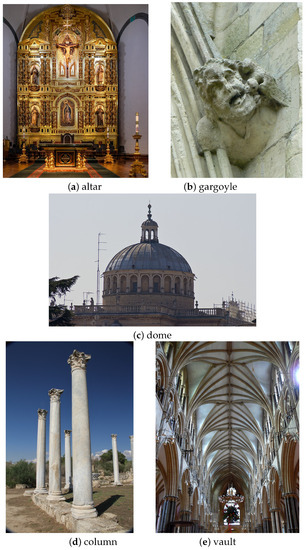
Figure 1.
Examples of images used for each of the five classes, in particular: (a) the altar, (b) the gargoyle, (c) the outer dome, (d) the column, and (e) the vault.
2.2. Methods
All experiments were performed in WEKA (Waikato Environment for Knowledge Analysis) [11], which is a free data mining software based on Java. Additionally, the CNN model was developed in Python v.3.7 with the use of the Keras library. The experiments were performed on a Windows machine with a 2.3 GHz processor and 8 GB of RAM.
Before applying the algorithms on the dataset, the feature extraction was performed using the imageFilters package, which contains different filters for image processing and is based on LIRE (Lucene Image REtrieval), a Java library for image retrieval. Three filters were applied on the dataset in order to extract feature descriptors from images, in particular the edge histogram filter, the color Layout filter, and the JPEG coefficients filter.
The edge histogram filter extracts the MPEG7 edge features from the images. Histograms are very useful in image processing, as they represent the composition of the image, regardless of the image rotation [12]. An edge histogram shows the directions of edges in an image, based on the frequency and brightness changes [12]. The edge histogram considers 5 types of edges in each local area (i.e., sub-image), including: vertical, horizontal, 45-degree diagonal, 135-degree diagonal, and non-directional edges [12,13] (Figure 2). Each sub-image consisted of 4 × 4 blocks totaling 16 blocks regardless of the image size; hence, the edge histogram was generated for each of these blocks, representing the distribution of the aforementioned edges in the observed sub-image [12,13].
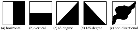
Figure 2.
Types of edge directions in the edge histogram, in particular (a) the horizontal edge, (b) the vertical edge, (c) the 45-degree edge, (d) the 135-degree edge, and (e) the non-directional edge.
The color layout features can be extracted from images by using the color layout filter in WEKA, where the image (on RGB color space) was divided into 64 blocks and the average color for each block was calculated. The features were computed based on the calculated average color. The color layout features represented the spatial distribution of colors [14], and were extracted from the images in two steps: (1) the selection of the representative color by partitioning the image and selecting the color and (2) the discrete cosine transform followed by the zigzag scanning and weighting [14].
The JPEG coefficients filter was used to extract JPEG coefficients from images. Feature extraction was performed by discarding information from images that was unnoticeable by humans. The image was split into parts of different frequencies based on the discrete cosine transform, after which the less important frequencies were excluded [15].
After the extraction of the features from the images, the dataset consisted of 307 attributes. The dataset was divided into 70% of images for training and 30% for testing the algorithms. This research tested and compared four algorithms for image classification: (i) MLP, (ii) Forest PA, (iii) AODE, and (iv) RSeslibKnn, followed by the additionally developed CNN model as a representation of the state-of-the-art techniques used in image classification.
Because the dataset consisted of 4000 images and 307 attributes, in order to improve performance in WEKA, the feature selection using the AttributeSelection filter was applied to extract the most important attributes from the set. The same attribute selection configuration was applied to all the algorithms. In particular, attribute search was performed using the best first method, while attribute evaluation was performed using CFS subset evaluator. In total, 89 attributes were extracted from the set and passed to the algorithm.
The MLP consists of a minimum of three layers: an input layer, a hidden layer, and an output layer, where each layer consists of neurons (nodes). It is an Artificial Neural Network (ANN) that uses a nonlinear activation function; hence, it is suitable for solving different types of problems. The neurons in each layer are connected to the neurons in the next layer, but at the same time, the neurons are not interconnected [16]. Furthermore, the nodes are connected by weights, and MLP uses backpropagation for training. One of the main advantages of MLP is that it does not make any assumptions regarding the distribution of data; hence, it can be used to model non-linear functions [17].
AODE is a classification method that was developed in order to slacken the naive Bayes independence assumptions, while at the same time obtaining good prediction accuracy with lower computational costs [18]. It estimates the probability of each class and creates a set of one dependence probability distribution estimators. These estimators are classifiers in which the probability of each value of the attribute is determined by other attributes and by the class to which the attribute belongs [19].
Forest PA is an algorithm developed in 2017 by [20]. It is a decision forest algorithm that is developed in order to overcome some of the shortcomings of the random forest algorithm and achieve better prediction power. Forest PA uses the full set of attributes, but at the same time, it assigns weights (i.e., penalties) to the attributes that already participated in the previous decision tree [20]. This algorithm uses the bootstrap sample by generating it from the training set, after which it develops a decision tree from that bootstrap sample using the attribute weights. The weights of the attributes used in the previous tree are, then, updated, and in the final step, the weights of the attributes that are not present in the previous tree are updated [20]. Forest PA is highly dependent on SimpleCart, which allows for minimal cost complexity pruning [21].
RSeslibKnn is the k-nearest neighbor classifier that uses a k optimization and is adequate for large sets of data, as it employs a fast neighbor search [22]. The algorithm first calculates a distance measure based on the weighted sum of distances and then creates an indexing tree. The weights can be calculated using three different methods: the distance based method, the accuracy based method, and a perceptron based method [22]. Classification is made by finding the k nearest neighbors in the set and voting for the decision. Three voting methods are supported, in particular the equally weighted method, the inverse distance weights, and the inverse square distance weights [22].
CNN is a neural network composed of the convolution and pooling layers, along with the standard type of layers that are used in different types of neural networks such as the fully connected layers. This type of neural network is mostly used for image processing, as it takes images as inputs and automatically extracts features from those images. The CNN usually consists of convolutional layers (each consisting of a predefined number of filters or nodes and kernel size). The convolutional layer is followed by the pooling layer, which is used to reduce the data dimensionality. Two types of pooling can be performed: max-pooling and average pooling. Max-pooling finds the maximum value from the image corresponding to the predefined kernel size, while average pooling finds the average of all the values. After image processing is done through these layers, the features from a two-dimensional matrix are transformed into a vector with the use of a flatten layer, and the obtained output is sent to the fully connected layer, which is the dense layer.
In terms of the parameter configuration, MLP used one hidden layer with 50 neurons and a learning rate set to 0.5, a momentum of 0.6, and the number of epochs set to 500. The batch size was set to 32, and the sigmoid activation function was used for both hidden and output layers. All attributes, including the target, were standardized. This configuration was chosen because it provided the best performance in terms of errors and accuracy.
AODE used the default WEKA parameters, while Forest PA included developing 30 trees in the forest. Furthermore, RSeslibKnn used the city and simple value difference as a distance measure, the inverse square distance as the voting method, and the distance based weighting method.
Lastly, the CNN architecture included four convolutional layers with 32 neurons in the first two layers, 64 neurons in the last two convolutional layers, one hidden layer with 128 neurons, and an output layer with 5 neurons corresponding to five classes. All convolutional and hidden layers used the hyperbolic tangent (tanh) activation function, which had an output in the range between −1 and 1, while the output layer used the softmax activation function. The kernel size of the convolutional layers was set to 3 × 3, while the pooling size in the pooling layer was set to 2 × 2. All pooling layers included max-pooling. Rmsprop was used as an optimizer, as it solves the problem with varying magnitudes of the gradient. The network used a dropout of 0.2. Lastly, in order to avoid overfitting, the early stopping regularization parameter was used with patience set to 3. The number of epochs was set to 50, but the training stopped after 18 epochs because there was no further improvement in the accuracy. The model used 80% of data for training and the rest of the data for validation.
2.3. Evaluation Metrics
In order to access the classification potential of each of the tested algorithms, several evaluation metrics were obtained. In particular, the percentage of correctly classified instances, precision, recall, F-score, kappa statistics, and ROC area were used to choose the best model.
The percentage of correctly classified instances represents the instances that are correctly classified by the algorithm, i.e., the accuracy. Precision is the proportion of instances that belong to the observed class and the total instances that are classified by the algorithm to that class, while recall presents the true positive rate of prediction [23]. The F-measure represents the classification accuracy based on the average of precision and recall values. The F-measure values closer to 1 indicate a better classification accuracy. This measure is calculated as follows:
Kappa is the measure of agreement and can be computed as [24]:
where represents the proportion of observed agreements and is the proportion of agreements by chance [24]. The agreement can be in an interval of 0–1, where the values in the range 0.81–1 represent almost perfect agreement, while values close to 0 represent poor agreement [24].
The area under the ROC curve represents the ratio of the true positives and the false positives. This value should be close to 1, indicating a perfect prediction, while the values under 0.5 indicate a random guess [25].
3. Results
The algorithms used in this study were first tested on the full set of data consisting of 307 attributes. The performance for each algorithm can be observed in Table 1. Based on the results, it can be observed that the MLP algorithm performed the best with 85% of correctly classified instances, followed by RSeslibKnn with 82% of correctly classified instances, AODE with 79%, and Forest PA with 78%. It can be also observed that the values of the kappa statistics, precision, recall, and the F-measure were better for the MLP algorithm, compared to the other tested algorithms.

Table 1.
The performance for each of the applied algorithms before attribute selection.
After applying the attribute selection, the algorithms were again trained and tested, and the obtained results for each algorithm are shown in Table 2. In general, considering each of the performance measures, the algorithm that obtained the best results was the MLP algorithm. In particular, MLP correctly classified 98.9% of instances, followed by AODE with 80.83%, RSeslibKnn with 80.67%, and Forest PA with 78.67% of correctly classified instances. In terms of the kappa statistics, MLP also obtained the best value of 0.986, which can be interpreted as an almost perfect agreement [24], followed by AODE (0.760), RSeslibKnn (0.758), and Forest PA (0.733), indicating a substantial agreement [24]. Furthermore, in terms of the F-measure, the best value was obtained for MLP (0.986), followed by RSeslibKnn (0.811), AODE (0.807), and Forest PA (0.797). Lastly, the values of the area under the ROC curve indicated an almost perfect prediction for the MLP (0.996), followed by AODE (0.965), Forest PA (0.959), and RSeslibKnn (0.879). All of these values demonstrated a strong classification power of each of the applied algorithms, with MLP and AODE performing the best in terms of different performance measures.
Table 2.
The performance for each of the applied algorithms after attribute selection.
In order to observe which of the classes the model classified wrongly, the confusion matrices were generated. The numbers in the diagonal represent the correctly classified instances, while other numbers in rows represent the misclassifications. Table 3 and Table 4 present the confusion matrices before and after applying the attribute selection. It was observed that the MLP and the Forest PA algorithms most correctly classified the dome images, while AODE and the RSeslibKnn most correctly classified the altar images (Table 3). In terms of misclassifications, MLP mostly misclassified the vault images, while AODE, Forest PA, and RSeslibKnn misclassified mainly the column images.
Table 3.
The confusion matrices for each algorithm, before attribute selection.
Table 4.
The confusion matrices for each algorithm, after attribute selection.
After applying the attribute selection, the confusion matrix in Table 4 was generated. It can be observed that the MLP algorithm mostly misclassified the column images, with 19 images in total being wrongly classified. The AODE algorithm mostly misclassified the column images, Forest PA mostly misclassified images belonging to the column and vault classes, while the RSeslibKnn algorithm mostly misclassified the vault images. Furthermore, in terms of the correctly classified images, the MLP, Forest PA, and RSeslibKnn algorithms most often correctly classified the dome images, while AODE most often correctly classified the altar and dome images.
Lastly, in order to fully observe the performance of these algorithms, the CNN model was developed in Python, and the obtained results are presented in Figure 3.
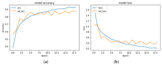
Figure 3.
The (a) accuracy and (b) loss results for the CNN model.
As observed, the CNN model performed well with an accuracy of 92.91%. Both training and validation loss had a decreasing trend achieving the value of 0.21 for training and 0.42 for validation in the last epoch.
4. Discussion
This study aimed to test and compare different algorithms for cultural heritage image classification tasks. In particular, a large dataset comprised of 4000 images classified into five categories was used, and several key findings were derived from the study: (i) the neural network based algorithms performed much better when classifying images compared to the other algorithms (both MLP and CNN obtained a relatively good accuracy); (ii) the k-nearest neighbor classifier performed better than the decision tree based classifier; (iii) all classifiers performed better after reducing the attribute number, except for the k-nearest neighbor classifier, which lost its prediction accuracy; and (iv) images of columns were most frequently misclassified, while images representing the dome were most frequently correctly classified by these algorithms.
As observed in the previous section, the MLP algorithm performed the best in terms of all performance measures. It achieved the highest classification accuracy, compared to the other tested algorithms, and performed the best in terms of the other performance measures, such as MAE, kappa statistics, and the ROC area. The results showed almost perfect classification agreement and accuracy. Moreover, the developed CNN model showed very good classification accuracy, confirming some of the findings from the literature. In particular, neural networks mostly perform better than other non-neural network algorithms used for classification tasks [26,27,28], especially when classifying images [29,30]. Furthermore, neural networks are more suitable for large sets of data due to the overfitting problems that can occur more often with small datasets. Even though the neural networks are more computationally intensive, they achieve better performances and allow extensive hyperparameter tuning. MLP was able to improve its classification accuracy after the attribute selection, hence confirming its flexibility, while CNN obtained very good accuracy without using any additional algorithm for performance improvement.
The RSeslibKnn algorithm performed slightly better than the Forest PA algorithm, which was used for the first time for image classification tasks. These findings supported some of the findings from the literature, as the k-nearest neighbor classification algorithm mostly performed better than decision tree based algorithms [31,32]. On the contrary, this was the only one from the tested algorithms that did not improve its performance after the attribute selection. This showed that RSeslibKnn was indeed better to use with larger sets of data, as its performance degraded with the decreased number of data in the dataset.
Forest PA achieved the lowest accuracy of classification, both before and after applying the attribute selection. In particular, the algorithm performed slightly better in the second case, but still maintained the accuracy below 80%. In terms of the ROC area value, it performed better than the k-nearest neighbor algorithm, indicating a good prediction potential. These results demonstrated the potential of the algorithm and its suitability for larger sets of data, particularly in terms of the attribute number.
Before the attribute selection, the AODE algorithm performed better than Forest PA, in terms of the percentage of correctly classified instances, but worse than MLP and RSeslibKnn. After selecting the attributes, AODE performed better than both Forest PA and RSeslibKnn. The algorithm mostly misclassified the column images, followed by the vault images.
The comparison of the tested algorithms in terms of the obtained accuracy is shown in Table 5. As observed, the best performance after the attribute selection was obtained for the MLP algorithm, while the lowest performance was obtained for the RSeslibKnn algorithm. The other two algorithms obtained a very small decrease in accuracy, after the attribute selection. As deep neural networks automatically scan images and extract features from them, no attribute selection was applied to this model; hence, CNN was compared to the accuracy of the applied algorithms both before and after the attribute selection. In these terms, the CNN achieved much better accuracy (92.91%) than all other models (before attribute selection), but it obtained a lower accuracy than the MLP model (after attribute selection).
Table 5.
The accuracy of each of the applied algorithms.
The results of this study can be used for developing new cultural heritage image classification models that will be more efficient and computationally compact. As image classification usually involves large sets of data, this task needs to be performed correctly and in a timely manner. Furthermore, image classification requires large computational resources; hence, working towards developing optimized models and classification methods is extremely important for future work.
5. Conclusions
This paper compared several classification algorithms for the purpose of cultural heritage image classification. In particular, MLP, AODE, Forest PA, and RSeslibKnn were tested before and after the attribute selection, in WEKA, while CNN was tested in Python on the full dataset with automatically extracted features. Overall, the best performance was achieved by the CNN algorithm, but considering the attribute selection, the MLP algorithm obtained the best classification accuracy. Other tested algorithms obtained no more than 82% accuracy.
This work confirmed that CNN are a much better choice for image classification, as they do not require manually extracting features from images, are easy to use, and can be thoroughly configured.
Funding
This research was supported by the Mathematical Institute of the Serbian Academy of Sciences and Arts (Project III44006).
Conflicts of Interest
The author declares no conflict of interest.
References
- Kurniawan, H.; Salim, A.; Suhartanto, H.; Hasibuan, Z.A. E-cultural heritage and natural history framework: An integrated approach to digital preservation. In Proceedings of the International Conference on Telecommunication Technology and Applications, St. Maarten, The Netherlands, 20–25 March 2011; pp. 177–182. [Google Scholar]
- Ivanova, K.; Dobreva, M.; Stanchev, P.; Totkov, G. Access to Digital Cultural Heritage: Innovative Applications of Automated Metadata Generation; Plovdiv University Publishing House “Paisii Hilendarski”: Plovdiv, Bulgaria, 2012. [Google Scholar]
- Llamas, J.; Lerones, P.M.; Medina, R.; Zalama, E.; Gómez-García-Bermejo, J. Classification of architectural heritage images using deep learning techniques. Appl. Sci. 2017, 7, 992. [Google Scholar] [CrossRef]
- Kambau, R.A.; Hasibuan, Z.A.; Pratama, M.O. Classification for Multiformat Object of Cultural Heritage using Deep Learning. In Proceedings of the 2018 IEEE Third International Conference on Informatics and Computing(ICIC), Palembang, Indonesia, 17–18 October 2018; pp. 1–7. [Google Scholar]
- Amato, G.; Falchi, F.; Gennaro, C. Fast image classification for monument recognition. J. Comput. Cult. Herit. (JOCCH). 2015, 8, 18. [Google Scholar] [CrossRef]
- Grilli, E.; Dininno, D.; Petrucci, G.; Remondino, F. From 2D to 3D supervised segmentation and classification for cultural heritage applications. Int. Arch. Photogramm. Remote Sens. Spat. Inf. Sci. 2018, 42, 399–406. [Google Scholar] [CrossRef]
- Meroño, J.E.; Perea, A.J.; Aguilera, M.J.; Laguna, A.M. Recognition of materials and damage on historical buildings using digital image classification. S. Afr. J. Sci. 2015, 111, 1–9. [Google Scholar] [CrossRef]
- Anzid, H.; Le Goic, G.; Bekkari, A.; Mansouri, A.; Mammass, D. Multimodal Images Classification using Dense SURF, Spectral Information and Support Vector Machine. Procedia Comput. Sci. 2019, 148, 107–115. [Google Scholar] [CrossRef]
- Ćosović, M.; Amelio, A.; Junuz, E. Classification Methods in Cultural heritage. In Proceedings of the 1st International Workshop on Visual Pattern Extraction and Recognition for Cultural Heritage Understanding Co-Located with 15th Italian Research Conference on Digital Libraries (IRCDL 2019), Pisa, Italy, 30 January 2019. [Google Scholar]
- Jankovic, R. Classifying Cultural Heritage Images by Using Decision Tree Classifiers in WEKA. In Proceedings of the 1st International Workshop on Visual Pattern Extraction and Recognition for Cultural Heritage Understanding Co-Located with 15th Italian Research Conference on Digital Libraries (IRCDL 2019), Pisa, Italy, 30 January 2019; pp. 119–127. [Google Scholar]
- Witten, I.H.; Frank, E.; Hall, M.A.; Pal, C.J. Data Mining: Practical Machine Learning Tools and Techniques; Morgan Kaufmann: Burlington, MA, USA, 2016. [Google Scholar]
- Won, C.S.; Park, D.K.; Park, S.J. Efficient Use of MPEG-7 Edge Histogram Descriptor. ETRI J. 2002, 24, 23–30. [Google Scholar] [CrossRef]
- Prajapati, N.; Nandanwar, A.K.; Prajapati, G. Edge histogram descriptor, geometric moment and Sobel edge detector combined features based object recognition and retrieval system. Int. J. Comput. Sci. Inf. Technol. 2016, 7, 0975–9646. [Google Scholar]
- Jalab, H.A. Image retrieval system based on color layout descriptor and Gabor filters. In Proceedings of the 2011 IEEE Conference on Open Systems, Langkawi, Malaysia, 25–28 September 2011; pp. 32–36. [Google Scholar]
- More, N.K.; Dubey, S. JPEG Picture Compression Using Discrete Cosine Transform. Int. J. Sci. Res. (IJSR) 2013, 2, 134–138. [Google Scholar]
- Pal, S.K.; Mitra, S. Multilayer perceptron, fuzzy sets, and classification. IEEE. Trans. Neural Netw. 1992, 3, 683–697. [Google Scholar] [CrossRef] [PubMed]
- Gardner, M.W.; Dorling, S. Artificial neural networks (the multilayer perceptron)—A review of applications in the atmospheric sciences. Atmos. Environ. 1998, 32, 2627–2636. [Google Scholar] [CrossRef]
- Webb, G.I.; Boughton, J.R.; Wang, Z. Not so naive Bayes: aggregating one-dependence estimators. Mach. Learn. 2005, 58, 5–24. [Google Scholar] [CrossRef]
- Cerquides, J.; De Mántaras, R.L. Robust Bayesian linear classifier ensembles. In Proceedings of the European Conference on Machine Learning, Porto, Portugal, 3–7 October 2005; Volume 3720, pp. 72–83. [Google Scholar]
- Adnan, M.N.; Islam, M.Z. Forest PA: Constructing a decision forest by penalizing attributes used in previous trees. Expert Syst. Appl. 2017, 89, 389–403. [Google Scholar] [CrossRef]
- Breiman, L.; Friedman, J.H.; Olshen, R.A.; Stone, C.J. Classification and Regression Trees; Wadsworth International Group: Belmont, CA, USA, 1984. [Google Scholar]
- Wojna, A.; Latkowski, R. Rseslib 3: Library of rough set and machine learning methods with extensible architecture. In Transactions on Rough Sets XXI; Springer: Berlin/Heidelberg, Germany, 2019; Volume 10810, pp. 301–323. [Google Scholar]
- Kumari, M.; Godara, S. Comparative Study of Data Mining Classification Methods in Cardiovascular Disease Prediction 1; CiteSeer: Princeton, NJ, USA, 2011. [Google Scholar]
- Sim, J.; Wright, C.C. The kappa statistic in reliability studies: Use, interpretation, and sample size requirements. Phys. Ther. 2005, 85, 257–268. [Google Scholar] [PubMed]
- Fan, J.; Upadhye, S.; Worster, A. Understanding receiver operating characteristic (ROC) curves. Can. J. Emerg. Med. 2006, 8, 19–20. [Google Scholar] [CrossRef] [PubMed]
- Ture, M.; Kurt, I.; Kurum, A.T.; Ozdamar, K. Comparing classification techniques for predicting essential hypertension. Expert Syst. Appl. 2005, 29, 583–588. [Google Scholar] [CrossRef]
- Kurt, I.; Ture, M.; Kurum, A.T. Comparing performances of logistic regression, classification and regression tree, and neural networks for predicting coronary artery disease. Expert Syst. Appl. 2008, 34, 366–374. [Google Scholar] [CrossRef]
- Tsoi, A.C.; Pearson, R. Comparison of three classification techniques: CART, C4.5 and Multi-Layer Perceptrons. In Proceedings of the Advances in Neural Information Processing Systems, Denver, CO, USA, 2–5 December 1991; pp. 963–969. [Google Scholar]
- Yogaswara, R.D.; Wibawa, A.D. Comparison of Supervised Learning Image Classification Algorithms for Food and Non-Food Objects. In Proceedings of the IEEE 2018 International Conference on Computer Engineering, Network and Intelligent Multimedia (CENIM), Surabaya, Indonesia, 26–27 November 2018; pp. 317–324. [Google Scholar]
- Siraj, F.; Salahuddin, M.A.; Yusof, S.A.M. Digital image classification for malaysian blooming flower. In Proceedings of the IEEE 2010 Second International Conference on Computational Intelligence, Modelling and Simulation, Tuban, Indonesia, 28–30 September 2010; pp. 33–38. [Google Scholar]
- Al Zorgani, M.; Ugail, H. Comparative Study of Image Classification using Machine Learning Algorithms; Technical Report; EasyChair: New York, NY, USA, 2018. [Google Scholar]
- Liu, H.; Cocea, M.; Ding, W. Decision tree learning based feature evaluation and selection for image classification. In Proceedings of the 2017 International Conference on Machine Learning and Cybernetics (ICMLC), Ningbo, China, 9–12 July 2017; Volume 2, pp. 569–574. [Google Scholar]


© 2019 by the author. Licensee MDPI, Basel, Switzerland. This article is an open access article distributed under the terms and conditions of the Creative Commons Attribution (CC BY) license (http://creativecommons.org/licenses/by/4.0/).