A Different Look at Polynomials within Man-Machine Interaction

Abstract

Undoubtedly, one of the most powerful applications that allow symbolic computations is Wolfram Mathematica. However, it turns out that sometimes Mathematica does not give the desired result despite its continuous improvement. Moreover, these gaps are not filled by many authors of books and tutorials. For example, our attempts to obtain a compact symbolic description of the roots of polynomials or coefficients of a polynomial with known roots using Mathematica have often failed and they still fail. Years of our work with theory, computations, and different kinds of applications in the area of polynomials indicate that an application ‘offering’ the user alternative methods of solving a given problem would be extremely useful. Such an application would be valuable not only for people who look for solutions to very specific problems but also for people who need different descriptions of solutions to known problems than those given by classical methods. Therefore, we propose the development of an application that would be not only a program doing calculations but also containing an interactive database about polynomials. In this paper, we present examples of methods and information which could be included in the described project.

1. Introduction

Computer-aided research has become very common in recent decades among many scientists in various fields of science. The use of computers has also been well-received by mathematicians. Many applications supporting and accelerating human work have been developed—mainly in the case of numerical and symbolic computations. Undoubtedly, one of the most powerful applications that allow symbolic computations is Wolfram Mathematica. However, it turns out that sometimes Mathematica does not give the desired result despite its continuous improvement (We used mainly version 8. Neither version 10 nor 12.1 gives more accessible forms of solutions to considered problems.). Moreover, many authors of books and tutorials do not fill the gaps. Our attempts to obtain a compact symbolic description of the roots of polynomials or coefficients of a polynomial with known roots (especially ones of trigonometric nature) using Mathematica have often failed and they still fail. Indeed, as users of this program, we are simply forced to do manual calculations. Still, we wrote ‘often’ before, since there are also some ‘computationally lucky’ or partially profitable cases.

To illustrate, let us consider finding roots of polynomials of the third degree. We believe that Mathematica uses almost exclusively Cardano formulae, i.e., it uses neither the trigonometric nor the hyperbolic formulae. We will illustrate the operation of Mathematica application on selected examples.

Let us first recall trigonometric formulae for roots of cubic polynomials. Let $\alpha ,\phi \in \mathbb{C}$ ( $\alpha ,\phi \in \mathbb{R}$, respectively). The complex (real, respectively) roots of the following polynomial

$$p\left(z\right)=z^3-3{\alpha }^{2}z+\left(2\cos \phi \right){\alpha }^3$$

(1)

are

$$z_1:=-2\alpha \cos \frac{\phi }{3},z_{2,3}:=\alpha \left(\cos \frac{\phi }{3}\pm \sqrt{3}\sin \frac{\phi }{3}\right).$$

Moreover, note that we have

$$\begin{array}{cc}\hfill p(z-\alpha )& =z^3-3\alpha z^2+3{\alpha }^{2}z-{\alpha }^3-3{\alpha }^{2}z+3{\alpha }^3+\left(2\cos \phi \right){\alpha }^3\hfill \\ \hfill & =z^3-3\alpha z^2+2(1+\cos \phi ){\alpha }^3=z^3-3\alpha z^2+4{\cos }^2\frac{\phi }{2}{\alpha }^3,\hfill \end{array}$$

and then the roots of this polynomial are $\alpha +z_{1,2,3}.$

Now, consider the following examples:

• In the case of polynomial $x^3-12x+11$ Mathematica gives us three roots in the following forms

  $$1,\frac{1}{2}\left(-1\pm 3\sqrt{5}\right).$$
  Meanwhile, the program we have implemented for determining roots in trigonometric form generates the following values

  $$-4\cos \left(\frac{1}{3}\arctan \frac{3\sqrt{15}}{11}\right),4\sin \left(\frac{\pi }{6}\pm \frac{1}{3}\arctan \frac{3\sqrt{15}}{11}\right).$$
  Surprisingly, that means that the following identity holds

  $$1=4\sin \left(\frac{\pi }{6}-\frac{1}{3}\arctan \frac{3\sqrt{15}}{11}\right)$$

  which was numerically checked by Mathematica.
• However, Mathematica cannot cope with the next polynomial $x^3-12x+13$. The roots given by Mathematica are as follows

  $$\begin{array}{cc}\hfill x_1& =-\frac{2\left(1+i\sqrt{3}\right)}{\sqrt[3]{\frac{1}{2}\left(-13+i\sqrt{87}\right)}}-\frac{1}{2}\left(1-i\sqrt{3}\right)\sqrt[3]{\frac{1}{2}\left(-13+i\sqrt{87}\right)},\hfill \end{array}$$

  (2)

  $$\begin{array}{cc}\hfill x_2& =-\frac{2\left(1-i\sqrt{3}\right)}{\sqrt[3]{\frac{1}{2}\left(-13+i\sqrt{87}\right)}}-\frac{1}{2}\left(1+i\sqrt{3}\right)\sqrt[3]{\frac{1}{2}\left(-13+i\sqrt{87}\right)},\hfill \end{array}$$

  (3)

  $$\begin{array}{cc}\hfill x_3& =\frac{4}{\sqrt[3]{\frac{1}{2}\left(-13+i\sqrt{87}\right)}}+\sqrt[3]{\frac{1}{2}\left(-13+i\sqrt{87}\right)}.\hfill \end{array}$$

  (4)
  Vaules of the roots obtained by our method are

  $$4\cos \left(\frac{1}{3}\arctan \frac{\sqrt{87}}{13}\right),4\sin \left(\frac{\pi }{6}\pm \frac{1}{3}\arctan \frac{\sqrt{87}}{13}\right).$$

  (5)
  Please note that to get them it was sufficient to write the complex numbers given in (2)–(4) in exponential form, namely

  $$\frac{1}{2}\left(-13+i\sqrt{87}\right)=-8e^{-i\arctan \frac{\sqrt{87}}{13}}.$$
  Now, since $-2e^{-\frac{i}{3}\arctan \frac{\sqrt{87}}{13}}$ is one of complex roots of $\sqrt[3]{\frac{1}{2}\left(-13+i\sqrt{87}\right)}$ we obtain:

  $$\begin{array}{cc}\hfill \frac{4}{\sqrt[3]{\frac{1}{2}\left(-13+i\sqrt{87}\right)}}+\sqrt[3]{\frac{1}{2}\left(-13+i\sqrt{87}\right)}& =-2e^{\frac{i}{3}\arctan \frac{\sqrt{87}}{13}}-2e^{-\frac{i}{3}\arctan \frac{\sqrt{87}}{13}}\hfill \\ \hfill & =-4\cos \left(\frac{1}{3}\arctan \frac{\sqrt{87}}{13}\right).\hfill \end{array}$$
  Let us notice that using Maple application we obtain the following relation between roots of discussed polynomial $x^3-12x+13$

  $$\begin{array}{c}-2\sin \left(\frac{1}{6}\arctan \left(\frac{13\sqrt{87}}{41}\right)+\frac{\pi }{6}\right)-2\sqrt{3}\cos \left(\frac{1}{6}\arctan \left(\frac{13\sqrt{87}}{41}\right)+\frac{\pi }{6}\right)\hfill \\ \hfill =-4\cos \left(\frac{1}{3}\arctan \left(\frac{\sqrt{87}}{13}\right)\right).\end{array}$$

  (6)
  The above follows from (5) and the fact that the sum of these roots is equal to zero. It is enough to notice that we have

  $$\begin{array}{c}4\left(\sin \left(\frac{\pi }{6}+t\right)+\sin \left(\frac{\pi }{6}-t\right)\right)=4\left(\sin \left(\frac{\pi }{6}+t\right)+\sin \left(\frac{\pi }{3}-\left(\frac{\pi }{6}+t\right)\right)\right)\hfill \\ \hspace{1em}\hspace{1em}\hspace{1em}\hspace{1em}=4\left(\sin \left(\frac{\pi }{6}+t\right)+\sin \frac{\pi }{3}\cos \left(\frac{\pi }{6}+t\right)-\cos \frac{\pi }{3}\sin \left(\frac{\pi }{6}+t\right)\right)\\ \hspace{1em}\hspace{1em}\hspace{1em}\hspace{1em}\hspace{1em}\hspace{1em}\hspace{1em}\hspace{1em}\hspace{1em}\hspace{1em}\hspace{1em}\hspace{1em}\hspace{1em}\hspace{1em}\hspace{1em}\hspace{1em}\hspace{1em}\hspace{1em}\hspace{1em}\hspace{1em}\hspace{1em}\hspace{1em}\hspace{1em}=2\sin \left(\frac{\pi }{6}+t\right)+2\sqrt{3}\cos \left(\frac{\pi }{6}+t\right),\end{array}$$

  where $t=\frac{1}{3}\arctan \frac{\sqrt{87}}{13}=\frac{1}{6}\arctan \frac{13\sqrt{87}}{41}$ by the following well-known formula for $x\in \mathbb{R}$

  $$\begin{array}{c}\hfill \arctan x=2\arctan \left(\frac{x}{1+\sqrt{1+x^2}}\right).\end{array}$$
• For the Perrin’s polynomial

  $$\mathrm{Per}\left(z\right)=z^3-z-1=\left(z-z_0^{-1}\right)\left(z-i\sqrt{z_0}{e}^{i\phi }\right)\left(z+i\sqrt{z_0}{e}^{-i\phi }\right),$$

  which is important in the theory of polynomials [1], we have the following description of its roots

  $$\begin{array}{cc}\hfill \sqrt[3]{18}{z}_0^{-1}& =\sqrt[3]{9+\sqrt{69}}+\sqrt[3]{9-\sqrt{69}},\hfill \\ \hfill i2\sqrt[3]{18}\sqrt{z_0}{e}^{i\phi }& =-\left(\sqrt[3]{9+\sqrt{69}}+\sqrt[3]{9-\sqrt{69}}\right)+\hfill \\ \hfill & +i\sqrt{3}\left(\sqrt[3]{9+\sqrt{69}}-\sqrt[3]{9-\sqrt{69}}\right),\hfill \end{array}$$

  obtained by manual calculations using Cardano formulae. This result is almost compatible with the one given by Mathematica

$$\begin{array}{cc}\hfill z_1& =\frac{\sqrt[3]{9-\sqrt{69}}+\sqrt[3]{9+\sqrt{69}}}{\sqrt[3]{2}{3}^{2/3}},\hfill \\ \hfill z_2& =\frac{i\left(\sqrt{3}+i\right)\sqrt[3]{9-\sqrt{69}}+\left(-1-i\sqrt{3}\right)\sqrt[3]{9+\sqrt{69}}}{2\sqrt[3]{2}{3}^{2/3}},\hfill \\ \hfill z_3& =\frac{\left(-1-i\sqrt{3}\right)\sqrt[3]{9-\sqrt{69}}+i\left(\sqrt{3}+i\right)\sqrt[3]{9+\sqrt{69}}}{2\sqrt[3]{2}{3}^{2/3}}.\hfill \end{array}$$

Based on examples (1)–(3) we conclude that Mathematica does not simplify symbolic forms of the roots of a given polynomial of a third degree enough to use them freely in further considerations. Usually, the description of the roots given by Mathematica demands additional action of the user.

A similar situation takes place in the case of finding coefficients of a polynomial with known roots. Mathematica computes only numerical approximations of the searched values. Because of that, all calculations have to be done manually, also these confirming the numerical results of Mathematica suggesting for example integer coefficients.

For example, factorization of the polynomial

$$\left(z-\tan \frac{2\pi }{9}\right)\left(z+\tan \frac{4\pi }{9}\right)\left(z-\tan \frac{8\pi }{9}\right)=z^3+3\sqrt{3}{z}^2-3z-\sqrt{3},$$

and identities

$$\tan \frac{2^k\pi }{9}=4\sin \frac{2^k\pi }{9}+{(-1)}^k\sqrt{3}$$

for $k=1,2,3$ were verified manually.

Remark 1.

As we already mentioned, many authors of books [2] and tutorials (available on-line) suggest using the classical Cardano formulae. The most popular argument is referring to classical books and great mathematicians (examples given by Leonhard Euler are still very popular). As an example let us consider the equation (This example is derived from Euler’s book Vollständige Anleitung zur Algebra, new edition, Lipsk, Ph. Reclam, p. 303—see [2].)

$$x^3-6x-40=0.$$

Since coefficients of the polynomial are integers then it is easy to see that $x=4$ is its root. We find the remaining roots by solving the equation of second order

$$x^2+4x+10=0,$$

which gives us $x=-2\pm i\sqrt{6}$. Without a doubt, in this case, Cardano formulae should not be used. The algorithm for finding solutions should take into account known tests (e.g., Eisenstein criterion for rational numbers).

Note also that, polynomials with rational roots can posses integer roots, for example the following equation

$$x^3+6.4x-1064=0$$

has integer solutions. Searching for the roots among integers is almost reflexive and is usually associated with the deep faith in the success of such research.

Years of work with theory, computations, and different kinds of applications in the area of polynomials confirmed our conviction that an application ‘offering’ the user alternative methods of solving a given problem would be extremely useful. Such an application would be valuable not only for people who look for solutions to very specific problems but also for people who need different descriptions of solutions to known problems than those given by classical methods. Therefore, we propose the development of the application which would be not only a program doing calculations but also containing an interactive database about polynomials. We want ‘human-computer’ interaction to play an important role in this project. This application should recognize and indicate the proper section in the database and even suggest calculations or next steps of research. Simultaneously, such an application should include less popular methods and algorithms described in the database to give the user not only theoretical but also practical knowledge. We plan to undertake such a project and we hope that users will be able to test the demo version of this application soon. At this moment we are waiting for receiving a web address at polsl.pl domain.

In this paper, we present examples of methods and information which could be included in the described project. We would like to stress the usefulness of computer-aided calculations on this topic.

2. Polynomials of a Fourth Degree

2.1. Lagrange’s Algorithm

The following algorithm for determining the roots of the polynomial Q is called Lagrange’s algorithm for polynomials of a fourth degree (see [3,4,5]). In our opinion, this is the most effective algebraic method for determining roots of polynomial of a fourth degree for giving the desired symbolic description of these roots.

Let us consider the following polynomial of a fourth degree

$$Q\left(x\right):=x^4+m{x}^3+n{x}^2+px+q.$$

(7)

We construct the resolvent cubic of $Q\left(x\right)$:

$$z^3+\alpha z^2+\beta z+\gamma ,$$

where:

$$\begin{array}{cc}\hfill \alpha & :=8n-3m^2,\hfill \\ \hfill \beta & :=3(m^4-16m^{2}n-16n^2+16mp-64q),\hfill \\ \hfill \gamma & :=-{(m^2-4m+8p)}^2.\hfill \end{array}$$

We find the complex roots $z_1$, $z_2$, $z_3$ of this polynomial. Then the complex roots of Q are as follows (see [4,6]):

$$x_k:=\frac{1}{4}\left(-m+\left\{\begin{array}{c}+\hfill \\ +\hfill \\ -\hfill \\ -\hfill \end{array}\right\}\sqrt{z_1}+{(-1)}^{k+1}\sqrt{z_2}+\left\{\begin{array}{c}+\hfill \\ -\hfill \\ -\hfill \\ +\hfill \end{array}\right\}\sqrt{z_3}\right)$$

for each $k=1,2,3,4$, where we choose respectively pairs of signs in brackets and we find the square roots of $z_1$, $z_2$, $z_3$ using the following algorithm:

—

if all the numbers $z_1$, $z_2$, $z_3$ are reals, then

$$\sqrt{z_k}:=\sqrt{|z_k|}\left(\frac{\mathrm{sgn}\left(z_k\right)+1}{2}+i\left|\frac{\mathrm{sgn}\left(z_k\right)-1}{2}\right|\right),$$

for every $k=1,2,3$;

—

if $z_1\in \mathbb{R}$, $z_2\in \mathbb{C}\backslash \mathbb{R}$ and $z_3=\overline{z_2}$, then

$$\begin{array}{cc}\hfill \sqrt{z_1}& :=\sqrt{|z_1|}\left(\frac{\mathrm{sgn}{z}_k+1}{2}+i\left|\frac{\mathrm{sgn}{z}_k-1}{2}\right|\right),\hfill \\ \hfill \sqrt{z_2}& :=\sqrt{|z_2|}\left(\cos \phi +i\sin \phi \right),\hfill \\ \hfill \sqrt{z_3}& :=\sqrt{|z_3|}\left(\cos \phi -i\sin \phi \right),\hfill \end{array}$$

where $\phi :=2\arctan \left(\frac{\Im z_2}{|z_2|+\Re z_2}\right)$.

Now, we present a few examples of the use of Algorithm 1.

Algorithm 1 Lagrange’s algorithm for polynomials of a fourth degree.

Input:$m,n,p,q$—coefficients of a given polynomial Q

1: Compute:

$\alpha :=8n-3m^2$

$\beta :=3(m^4-16m^{2}n-16n^2+16mp-64q)$

$\gamma :=-{(m^2-4m+8p)}^2$

2: Find roots $z_1,z_2,z_3$ of polynomial $z^3+\alpha z^2+\beta z+\gamma$, e.g., by Cardano formulae.

3: if $z_1,z_2,z_3\in \mathbb{R}$ then

4:  for $1\le k\le 3$ do

${\displaystyle r_k:=\sqrt{|z_k|}\left(\frac{\mathrm{sgn}\left(z_k\right)+1}{2}+i\left|\frac{\mathrm{sgn}\left(z_k\right)-1}{2}\right|\right)}$

5:  end for

6: else

7:  if $z_1\in \mathbb{R},z_2\in \mathbb{C}\backslash \mathbb{R},z_3=\overline{z_2}$  then

${\displaystyle \phi :=2\arctan \left(\frac{\Im \left(z_2\right)}{|z_2|+\Re \left(z_2\right)}\right)}$

${\displaystyle r_1:=\sqrt{|z_1|}\left(\frac{\mathrm{sgn}\left(z_1\right)+1}{2}+i\left|\frac{\mathrm{sgn}\left(z_1\right)-1}{2}\right|\right)}$

${\displaystyle r_2:=\sqrt{|z_2|}\left(\cos \phi +i\sin \phi \right)}$

${\displaystyle r_3:=\sqrt{|z_3|}\left(\cos \phi -i\sin \phi \right)}$

8:  end if

9: end if

10: ${\displaystyle x_1:=\frac{1}{4}\left(-m+r_1+r_2+r_3\right)}$

11: ${\displaystyle x_2:=\frac{1}{4}\left(-m+r_1-r_2-r_3\right)}$

12: ${\displaystyle x_3:=\frac{1}{4}\left(-m-r_1+r_2-r_3\right)}$

13: ${\displaystyle x_4:=\frac{1}{4}\left(-m-r_1-r_2+r_3\right)}$

Output:$x_1,x_2,x_3,x_4$—the roots of polynomial Q

2.1.1. Angle $\frac{\pi }{20}$

First, let us consider the polynomial

$$\begin{array}{cc}\hfill p\left(x\right)& =\left(x-2\cos \frac{\pi }{20}\right)\left(x-2\cos \frac{3\pi }{20}\right)\left(x-2\cos \frac{9\pi }{20}\right)\left(x+2\cos \frac{7\pi }{20}\right)\hfill \\ \hfill & =\prod _{k=0}^3\left(x-2\cos \frac{3^k\pi }{20}\right)=x^4-\sqrt{10}{x}^3+x^2+\sqrt{10}x-1,\hfill \end{array}$$

(8)

where

$$\left\{\begin{array}{c}+\hfill \\ +\hfill \\ -\hfill \\ +\hfill \end{array}\right\}2\cos \frac{3^k\pi }{20}=\sqrt{2+\left\{\begin{array}{c}+\\ +\\ -\\ -\end{array}\right\}\sqrt{\frac{5+{(-1)}^k\sqrt{5}}{2}}},$$

(9)

for each $k=0,1,2,3$ and respectively chosen pairs of signs. Please note that

$$p\left(x\right)-{\left(x^2-\sqrt{\frac{5}{2}}x-\frac{3}{4}\right)}^2=-\frac{25}{16}+\frac{1}{2}\sqrt{\frac{5}{2}}x,$$

which implies (after substituting $2\cos \frac{3^k\pi }{20}$ for x, $k=0,1,2,3$)

$$\begin{array}{cc}\hfill \sqrt{\frac{25}{16}-\sqrt{\frac{5}{2}}\cos \frac{\pi }{20}}& +\sqrt{\frac{25}{16}+\sqrt{\frac{5}{2}}\cos \frac{7\pi }{20}}\hfill \\ \hfill & =\sqrt{\frac{25}{16}-\sqrt{\frac{5}{2}}\cos \frac{3\pi }{20}}+\sqrt{\frac{25}{16}-\sqrt{\frac{5}{2}}\cos \frac{9\pi }{20}}.\hfill \end{array}$$

(10)

Let us also notice that ${\displaystyle \sum _{k=0}^3}\cos \frac{3^k\pi }{20}=\frac{\sqrt{10}}{2}$. Moreover, we have

$$\begin{array}{cc}\hfill \sqrt{\frac{25}{16}+\sqrt{\frac{5}{2}}\cos \frac{7\pi }{20}}& -\sqrt{\frac{25}{16}-\sqrt{\frac{5}{2}}\cos \frac{3\pi }{20}}\hfill \\ \hfill & =\sqrt{\frac{25}{16}-\sqrt{\frac{5}{2}}\cos \frac{9\pi }{20}}-\sqrt{\frac{25}{16}-\sqrt{\frac{5}{2}}\cos \frac{\pi }{20}}=\frac{\sqrt{5}}{2},\hfill \end{array}$$

which follows from the following identity (easy to obtain e.g., from (9))

$$\sqrt{5-8\sqrt{\frac{2}{5}}\cos \frac{3^k\pi }{20}}=\sqrt{\frac{2}{\sqrt{5}}-{(-1)}^{k}2}+{(-1)}^{\frac{1}{2}(k+1)(k+2)}$$

for every $k=0,1,2,3$. Using Lagrange’s algorithm for the polynomial $p\left(x\right)$ we get the following description of its roots:

$$\begin{array}{cccc}\hfill 24\cos \frac{\pi }{20}& =3a_1+b-c,\hfill & \hfill \hspace{1em}\hspace{1em}\hspace{1em}24\cos \frac{3\pi }{20}& =3a_1-b+c,\hfill \\ \hfill 24\cos \frac{9\pi }{20}& =3a_2+b+c,\hfill & \hfill \hspace{1em}\hspace{1em}\hspace{1em}24\cos \frac{7\pi }{20}& =-3a_2+b+c,\hfill \end{array}$$

where

$$\begin{array}{cc}\hfill a_1& =\sqrt{10}+\sqrt{10+4\sqrt{5}},a_2=2\sqrt{10}-a_1,\hfill \\ \hfill b& =\sqrt{66-24\sqrt{19}\sin \left(\frac{\pi }{6}-\frac{1}{3}\arctan \frac{3\sqrt{15}}{82}\right)},\hfill \\ \hfill c& =\sqrt{66-24\sqrt{19}\sin \left(\frac{\pi }{6}+\frac{1}{3}\arctan \frac{3\sqrt{15}}{82}\right)}.\hfill \end{array}$$

This implies the following set of original equalities

$$\begin{array}{cc}\hfill \frac{66-b^2}{24}& =\sqrt{19}\sin \left(\frac{\pi }{6}-\frac{1}{3}\arctan \frac{3\sqrt{15}}{82}\right)=2,\hfill \\ \hfill \sqrt{5-2\sqrt{5}}& =\frac{c}{3\sqrt{2}}=\sqrt{\frac{11}{3}-\frac{4}{3}\sqrt{19}\sin \left(\frac{\pi }{6}+\frac{1}{3}\arctan \frac{3\sqrt{15}}{82}\right)}\hfill \end{array}$$

and

$$\begin{array}{cc}\hfill \frac{66-c^2}{12}=2\sqrt{19}\sin \left(\frac{\pi }{6}+\frac{1}{3}\arctan \frac{3\sqrt{15}}{82}\right)& =3\sqrt{5}-2,\hfill \end{array}$$

$$\begin{array}{cc}\hfill 2\sqrt{19}\cos \left(\frac{1}{3}\arctan \frac{3\sqrt{15}}{82}\right)=3\sqrt{5}+2,& 2\sqrt{57}\sin \left(\frac{1}{3}\arctan \frac{3\sqrt{15}}{82}\right)=3(\sqrt{5}-2),\hfill \\ \hfill \sqrt{5+2\sqrt{5}}+\sqrt{5-2\sqrt{5}}=\sqrt{2(5+\sqrt{5})}& =1-\sqrt{5}+4\sqrt{1+\frac{1}{2}\sqrt{\frac{5-\sqrt{5}}{2}}}.\hfill \end{array}$$

(11)

2.1.2. Polynomial Connected with a Pisot Number

Another interesting polynomial we tested is as follows

$$\begin{array}{cc}\hfill Q\left(x\right)& =x^4-2x^3+x-1={(x^2-x)}^2-(x^2-x)-1=\left(x^2-x-\phi \right)\left(x^2-x+\frac{1}{\phi }\right)\hfill \\ \hfill & =\left(x-\frac{1-\sqrt{3+2\sqrt{5}}}{2}\right)\left(x-\frac{1+\sqrt{3+2\sqrt{5}}}{2}\right)\times \hfill \\ \hfill & \times \left(x-\frac{1-i\sqrt{-3+2\sqrt{5}}}{2}\right)\left(x-\frac{1+i\sqrt{-3+2\sqrt{5}}}{2}\right).\hfill \end{array}$$

In this case, we obtained the same factorization (i.e., the same formula) by using Lagrange’s algorithm as well as using Mathematica. Let us note that the following notable result was proved in [1]: the number $\left(1+\sqrt{3+2\sqrt{5}}\right)/2$ (the polynomial Q is its minimal polynomial) is the only Pisot number such that its four different conjugations ${\alpha }_1$, ${\alpha }_2$, ${\alpha }_3$, ${\alpha }_4$ satisfy the relation ${\alpha }_1+{\alpha }_2={\alpha }_3+{\alpha }_4$. Suppose that $z_0\in \mathbb{C}$ is an algebraic number and $Q\in \mathbb{C}\left[z\right]$ is the minimal polynomial of $z_0$. Then all roots of the polynomial Q are called conjugations of $z_0$. It is assumed that $z_0$ itself is included in the set of conjugates of $z_0$. Let us recall that the Pisot number $\alpha >1$ is an integer algebraic number such that all its conjugations over Q, except itself, are contained in the complex unit circle $\left|z\right|<1$. See also [7].

3. Polynomials of a Fifth Degree

3.1. Spearman-Williams Theorem on the Factorization of Polynomials $x^5+ax+b$, $a,b\in \mathbb{Q}\backslash \left\{0\right\}$

This section is based on the following papers [8,9,10], see also [11,12]. The following theorem holds.

Theorem 1

(B.K. Spearman, K.S. Williams [8]). Let $a,b\in \mathbb{Q}\backslash \left\{0\right\}$ and suppose that $x^5+ax+b$ is irreducible over $\mathbb{Q}\left[x\right]$. Then the following equation

$$x^5+ax+b=0$$

(12)

is solvable by radicals if and only if there exist rational numbers $\epsilon =\pm 1$, $c\ge 0$ and $e\ne 0$ such that

$$a=\frac{5e^4(3-4\epsilon c)}{c^2+1},b=\frac{-4e^5(11\epsilon +2c)}{c^2+1}.$$

(13)

In this case, the following numbers are solutions to the Equation (12)

$$x_j=e\left({\omega }^j{u}_1+{\omega }^{2j}{u}_2+{\omega }^{3j}{u}_3+{\omega }^{4j}{u}_4\right),j=0,1,2,3,4,$$

(14)

where $\omega :=\exp \frac{2\pi i}{5}$ and

$$u_1={\left(\frac{v_1^2{v}_3}{D^2}\right)}^{1/5},u_2={\left(\frac{v_3^2{v}_4}{D^2}\right)}^{1/5},u_3={\left(\frac{v_2^2{v}_1}{D^2}\right)}^{1/5},u_4={\left(\frac{v_4^2{v}_2}{D^2}\right)}^{1/5},$$

where

$$\begin{array}{cccc}\hfill v_1& =\sqrt{D}+\sqrt{D-\epsilon \sqrt{D}},\hfill & \hfill \hspace{1em}\hspace{1em}\hspace{1em}{v}_2& =-\sqrt{D}-\sqrt{D+\epsilon \sqrt{D}},\hfill \\ \hfill v_3& =-\sqrt{D}+\sqrt{D+\epsilon \sqrt{D}},\hfill & \hfill \hspace{1em}\hspace{1em}\hspace{1em}{v}_4& =\sqrt{D}-\sqrt{D-\epsilon \sqrt{D}},\hfill \end{array}$$

and

$$D=c^2+1.$$

Remark 2.

The Formula (14) can be reformulated (after simple calculations) as follows

$$x_j=e\left({\omega }^j{u}_1+\frac{{\omega }^{2j}{u}_1^2\sqrt{D}\sqrt[5]{\epsilon }}{v_1}+\frac{{\omega }^{3j}{u}_1^{3}D}{v_1{v}_3}-\frac{{\omega }^{4j}{u}_1^4\sqrt{D^3}}{v_1^2{v}_3}\sqrt[5]{\frac{\epsilon }{D}}\right)$$

for $j=0,1,2,3,4$.

Notice that from the Formula (13) we immediately obtain the following corollary.

Corollary 1.

Let $a\in \mathbb{Q}\backslash \left\{0\right\}$ and let b be a positive rational number. If the polynomial $x^5+ax+b$ is irreducible over $\mathbb{Q}\left[x\right]$ and the equation $x^5+ax+b=0$ is solvable by radicals then the polynomial $x^5+ax-b$ is also irreducible over $\mathbb{Q}\left[x\right]$ as well and the equation $x^5+ax-b=0$ is solvable by radicals.

As an example of the application of Algorithm 2, we find complex roots of the polynomial generated for $\epsilon =1$, $c=\frac{2}{11}$ and $e=-1$, that is the polynomial

$$x^5+11x+44.$$

The roots are (we used Mathematica for calculations):

$$\begin{array}{cc}\hfill x_0& =\lambda ({\xi }_1-{\xi }_2-{\xi }_3-{\xi }_4)\approx -1.87775,\hfill \\ \hfill x_1& =-\lambda \left(e^{\frac{3\pi i}{5}}{\xi }_1+e^{\frac{2\pi i}{5}}{\xi }_2+e^{\frac{4\pi i}{5}}{\xi }_3-e^{\frac{\pi i}{5}}{\xi }_4\right)\approx 1.80012-1.44746i,\hfill \\ \hfill x_2& =-\lambda \left(e^{\frac{\pi i}{5}}{\xi }_1+e^{\frac{4\pi i}{5}}{\xi }_2-e^{\frac{3\pi i}{5}}{\xi }_3+e^{\frac{2\pi i}{5}}{\xi }_4\right)\approx -0.861241-1.9105i,\hfill \\ \hfill x_3& ={\overline{x}}_2,x_4={\overline{x}}_1,\hfill \end{array}$$

where $\lambda =-\sqrt[5]{11/5^4}$ and

$$\begin{array}{cc}\hfill {\xi }_k& :={\left({(-1)}^{k+1}(50\sqrt{5}-75)+\sqrt{18125-6169\sqrt{5}}\right)}^{1/5},\hfill \\ \hfill {\xi }_l& :={\left(50\sqrt{5}+75+{(-1)}^l\sqrt{18125+6169\sqrt{5}}\right)}^{1/5},\hfill \end{array}$$

for $k=1,2$ and $l=3,4$.

Algorithm 2 An algorithm generating polynomials that satisfy the assumptions of Theorem 1 and calculating their roots.

Input:c—a non-negative rational number, e—a rational number not equal to 0, $\epsilon$—is equal to 1 or $-1$

1: Compute:

${\displaystyle a:=\frac{5e^4(3-4\epsilon c)}{c^2+1},b:=\frac{-4e^5(11\epsilon +2c)}{c^2+1}}$

$\omega :=\exp \frac{2\pi i}{5}$

$D:=c^2+1$

${\displaystyle v_1:=\sqrt{D}+\sqrt{D-\epsilon \sqrt{D}},v_2:=-\sqrt{D}-\sqrt{D+\epsilon \sqrt{D}},}$

${\displaystyle v_3:=-\sqrt{D}+\sqrt{D+\epsilon \sqrt{D}},v_4:=\sqrt{D}-\sqrt{D-\epsilon \sqrt{D}},}$

${\displaystyle u_1:={\left(\frac{v_1^2{v}_3}{D^2}\right)}^{1/5},u_2:={\left(\frac{v_3^2{v}_4}{D^2}\right)}^{1/5},u_3:={\left(\frac{v_2^2{v}_1}{D^2}\right)}^{1/5},u_4:={\left(\frac{v_4^2{v}_2}{D^2}\right)}^{1/5}}$

2: for $0\le j\le 4$  do

${\displaystyle x_j:=e\left({\omega }^j{u}_1+{\omega }^{2j}{u}_2+{\omega }^{3j}{u}_3+{\omega }^{4j}{u}_4\right)}$

3: end for

4: function Q(x)       ▹ Symbolically: ${\displaystyle Q\left(x\right):=x^5+ax+b}$

return $x^5+ax+b$  and $x_1,x_2,x_3,x_4$

5: end function

Output:Q—a polynomial satisfying the assumptions of Theorem 1, $x_0,x_1,x_2,x_3,x_4$—the roots of polynomial Q

3.2. Basically Different, Irreducible, Solvable, Spearman-Williams Trinomials of a Fifth Degree: $x^5+a{x}^2+b$, $a,b\in \mathbb{Q}\backslash \left\{0\right\}$

Let $f\in \mathbb{Q}\left[x\right]$ be an irreducible polynomial. If the equation $f\left(x\right)=0$ is solvable by radicals then the polynomial f is called solvable. B.K. Spearman and K.S. Williams in [9] (see also [10]) proved that there exist only five substantially different, irreducible, and solvable trinomials of a fifth degree of the form $x^5+a{x}^2+b$, where $a,b\in \mathbb{Q}$. They are as follows, see also [8,13]

$$\begin{array}{cc}\hfill x^5+5& x^2+3,x^5+5x^2-15,x^5+25x^2+300,\hfill \\ \hfill & x^5+100x^2+1000,x^5+250x^2+625.\hfill \end{array}$$

As an example, we present here the roots of three of the above polynomials. These roots are described by the following formula

$$x_j={\omega }^j{u}_1+{\omega }^{2j}{u}_2+{\omega }^{3j}{u}_3+{\omega }^{4j}{u}_{4}j=0,1,2,3,4,$$

where $\omega$ is a complex fifth root of unity and $u_1,u_2,u_3,u_4$ are given as follows:

• $(a,b)=(5,3)$

  $$\begin{array}{cc}\hfill u_1& ={\left(-\frac{1}{4}+\frac{1}{20}\sqrt{5}-\frac{1}{100}\sqrt{150+30\sqrt{5}}+\frac{1}{50}\sqrt{150-30\sqrt{5}}\right)}^{\frac{1}{5}},\hfill \\ \hfill u_2& ={\left(-\frac{1}{4}-\frac{1}{20}\sqrt{5}-\frac{1}{50}\sqrt{150+30\sqrt{5}}-\frac{1}{100}\sqrt{150-30\sqrt{5}}\right)}^{\frac{1}{5}},\hfill \\ \hfill u_3& ={\left(-\frac{1}{4}-\frac{1}{20}\sqrt{5}+\frac{1}{50}\sqrt{150+30\sqrt{5}}+\frac{1}{100}\sqrt{150-30\sqrt{5}}\right)}^{\frac{1}{5}},\hfill \\ \hfill u_4& ={\left(-\frac{1}{4}+\frac{1}{20}\sqrt{5}+\frac{1}{100}\sqrt{150+30\sqrt{5}}-\frac{1}{50}\sqrt{150-30\sqrt{5}}\right)}^{\frac{1}{5}};\hfill \end{array}$$
• $(a,b)=(5,-15)$

  $$\begin{array}{c}\hfill u_1={\left(\frac{5}{4}+\frac{13}{20}\sqrt{5}-\frac{7}{100}\sqrt{750+330\sqrt{5}}\right)}^{\frac{1}{5}},\\ \hfill u_2={\left(\frac{5}{4}-\frac{13}{20}\sqrt{5}-\frac{7}{100}\sqrt{750-330\sqrt{5}}\right)}^{\frac{1}{5}},\\ \hfill u_3={\left(\frac{5}{4}-\frac{13}{20}\sqrt{5}+\frac{7}{100}\sqrt{750-330\sqrt{5}}\right)}^{\frac{1}{5}},\\ \hfill u_4={\left(\frac{5}{4}+\frac{13}{20}\sqrt{5}+\frac{7}{100}\sqrt{750+330\sqrt{5}}\right)}^{\frac{1}{5}};\end{array}$$
• $(a,b)=(100,1000)$

  $$\begin{array}{c}\hfill u_1=-2^{\frac{6}{5}},u_2=-2^{\frac{7}{5}},u_3=2^{\frac{3}{5}},u_4=-2^{\frac{4}{5}}.\end{array}$$

4. Polynomials of a Sixth Degree

We want the new application to contain also a database of factorizations including only the polynomials of a special form. In such situations, general methods are often not effective enough or we obtain the results in undesirable forms. However, our application would ‘encourage’ the user to individually choose of the method of solving a given problem. Below we present a few examples of such special polynomials.

4.1. A Product of Two Polynomials of a Third Degree

4.1.1. Factorization of the Polynomials of Sine-Type for the Angle $\frac{2\pi }{21}$

We have the following factorization

$$\begin{array}{cc}\hfill & \left(x^3+\frac{\sqrt{a}-\sqrt{b}}{2}{x}^2+\frac{-a-\sqrt{ab}}{2}x+\frac{\sqrt{a}+\sqrt{b}}{2}\right)\left(x^3+\frac{-\sqrt{a}-\sqrt{b}}{2}{x}^2+\frac{-a+\sqrt{ab}}{2}x+\frac{-\sqrt{a}+\sqrt{b}}{2}\right)\hfill \\ \hfill & =x^6-\sqrt{b}{x}^5+\frac{b-5a}{4}{x}^4+(a+1)\sqrt{b}{x}^3+\frac{(a-2)(a+b)}{4}{x}^2+\frac{b-a}{4},\hfill \end{array}$$

where $a,b\in \mathbb{C};$ e.g., for $a=3$, $b=7$ we get

$$\begin{array}{cc}\hfill & x^6-\sqrt{7}{x}^5-2x^4+4\sqrt{7}{x}^3-8x^2+1\hfill \\ \hfill & =\left(x^3+\frac{\sqrt{3}-\sqrt{7}}{2}{x}^2-\frac{3+\sqrt{21}}{2}x+\frac{\sqrt{3}+\sqrt{7}}{2}\right)\left(x^3-\frac{\sqrt{3}+\sqrt{7}}{2}{x}^2+\frac{-3+\sqrt{21}}{2}x+\frac{-\sqrt{3}+\sqrt{7}}{2}\right)\hfill \\ \hfill & =\left(\left(x-2\sin \frac{2\pi }{21}\right)\left(x-2\sin \frac{8\pi }{21}\right)\left(x-2\sin \frac{32\pi }{21}\right)\right)\times \hfill \\ \hfill & \times \left(\left(x-2\sin \frac{4\pi }{21}\right)\left(x-2\sin \frac{16\pi }{21}\right)\left(x-2\sin \frac{64\pi }{21}\right)\right)\hfill \\ \hfill & =\left(\prod _{k=0}^2\left(x-2\sin \frac{2·4^k\pi }{21}\right)\right)\left(\prod _{k=1}^3\left(x-2\sin \frac{4^k\pi }{21}\right)\right)=\prod _{k=1}^6\left(x-2\sin \frac{2^k\pi }{21}\right).\hfill \end{array}$$

4.1.2. Factorization of the Polynomials of Cosine-Type for the Angle $\frac{2\pi }{21}$

We have the following factorization

$$\begin{array}{cc}\hfill & \left(x^3-\frac{1+\sqrt{a}}{2}{x}^2-\frac{1-\sqrt{a}}{2}x-\frac{c-\sqrt{a}}{2}\right)\left(x^3-\frac{1-\sqrt{a}}{2}{x}^2-\frac{1+\sqrt{a}}{2}x-\frac{c+\sqrt{a}}{2}\right)\hfill \\ \hfill & =x^6-x^5-\frac{3+a}{4}{x}^4+\left(\frac{a+1}{2}-c\right)x^3+\frac{1+a+2c}{4}{x}^4+\frac{c-a}{2}x+\frac{c^2-a}{4}\hfill \end{array}$$

for every $a,c\in \mathbb{C}$. If $c=\sqrt{a+4}$ then $\frac{c^2-a}{4}=1$, e.g., for $a=21$, $b=4$ we obtain

$$\begin{array}{cc}\hfill & \prod _{k=1}^6\left(x-2\cos \frac{2^k\pi }{21}\right)\hfill \\ & =\left(x^3-\frac{1+\sqrt{21}}{2}{x}^2-\frac{1-\sqrt{21}}{2}x-\frac{5-\sqrt{21}}{2}\right)\left(x^3-\frac{1-\sqrt{21}}{2}{x}^2-\frac{1+\sqrt{21}}{2}x-\frac{5+\sqrt{21}}{2}\right)\hfill \\ \hfill & =x^6-x^5-6x^4+6x^3+8x^2-8x+1.\hfill \end{array}$$

Let us mention that the above polynomial is a minimal polynomial for $2\cos \frac{2\pi }{21}$.

4.1.3. Factorization of the Polynomials of Cosine-Type for the Angle $\frac{2\pi }{13}$

We have the following factorization

$$\begin{array}{cc}\hfill & \left(z^3+\frac{b-\sqrt{a}}{2}{z}^2-z+\frac{\sqrt{a}+c}{2}\right)\left(z^3+\frac{b+\sqrt{a}}{2}{z}^2-z-\frac{\sqrt{a}+c}{2}\right)\hfill \\ \hfill & ={\left(z^3+\frac{b}{2}{z}^2-z\right)}^2-{\left(\frac{\sqrt{a}+c}{2}-\frac{\sqrt{a}}{2}{z}^2\right)}^2\hfill \\ \hfill & =z^6+b{z}^5+\left(\frac{b^2-a}{4}-2\right)z^4-b{z}^3+\left(1+\frac{a+c\sqrt{a}}{2}\right)z^2-{\left(\frac{\sqrt{a}+c}{2}\right)}^2,\hfill \end{array}$$

where $a,b,c\in \mathbb{C}$; e.g., for $a=13$, $b=1$, $c=3$ we get

$$\begin{array}{cc}\hfill \prod _{k=1}^6& \left(z-2\cos \frac{2^k\pi }{13}\right)=\left(z^3+\frac{1-\sqrt{13}}{2}{z}^2-z+\frac{\sqrt{13}+3}{2}\right)\left(z^3+\frac{1+\sqrt{13}}{2}{z}^2-z-\frac{\sqrt{13}+3}{2}\right)\hfill \\ \hfill & =z^6+z^5-5z^4-z^3+\left(1+\frac{13+3\sqrt{13}}{2}\right)z^2-{\left(\frac{3+\sqrt{13}}{2}\right)}^2.\hfill \end{array}$$

4.2. Trinomials of a Sixth Degree

First, let us recall an important definition.

Definition 1.

If the polynomial $p\in \mathbb{Q}\left[x\right]$ is a product of r irreducible polynomials over $\mathbb{Q}$ of degrees $n_1,n_2,\dots ,n_r$, respectively, $n_1\le n_2\le \dots \le n_r$, then we say that the polynomial $p\in \mathbb{Q}\left[x\right]$ has reducibility type $(n_1,n_2,\dots ,n_r)$.

Now we present three main theorems (which come from [14]) on trinomials of a sixth degree with certain reducibility types.

Theorem 2.

There are infinitely many trinomials $x^6+Ax+B\in \mathbb{Q}\left[x\right]$ with reducibility type $(1,2,3)$. There are no trinomials $x^6+Ax+B\in \mathbb{Q}\left[x\right]$ with reducibility type $(1,1,1,3)$ or $(1,1,2,2)$ or $(2,2,2)$.

Theorem 3.

1. 

There is no trinomial $x^6+A{x}^2+B\in \mathbb{Q}\left[x\right]$ with reducibility type $(1,2,3)$.

2. 

If the trinomial $x^6+A{x}^2+B\in \mathbb{Q}\left[x\right]$ has reducibility type $(2,2,2)$ then either

(a) 

$${\displaystyle (A,B)=\left(-s^2-sv-v^2,-sv(s+v)\right)}$$

where $s,v\in \mathbb{Q}$, $sv(s+v)\ne 0$, which implies factorization

$$x^6+A{x}^2+B=\left(x^2+s\right)\left(x^2+v\right)\left(x^2-s-v\right),$$

(b) 

or (up to scaling of a variable) we have

$$(A,B)=\left(-(v-1)(3v-1),-v^2(2v-1)\right),$$

where $v\in \mathbb{Q}\backslash \left\{0,1,\frac{1}{2},\frac{1}{3}\right\}$, which implies factorization

$$x^6+A{x}^2+B=\left(x^2+x+v\right)\left(x^2-x+v\right)\left(x^2-2v+1\right).$$

Theorem 4.

1. 

If the trinomial $x^6+A{x}^3+B\in \mathbb{Q}\left[x\right]$ has reducibility type $(2,2,2)$ then (up to scaling of a variable) we have

$$A=-27u(u+1),B=27\left(u^2+u+1\right),$$

where $u\in \mathbb{Q}\backslash \left\{0,-1,-\frac{1}{2}\right\}$, which implies factorization

$$\begin{array}{cc}\hfill x^6-27u& (u+1)x^3+27{\left(u^2+u+1\right)}^3=\left(x^2+3x+3\left(u^2+u+1\right)\right)\times \hfill \\ \hfill & \times \left(x^2-3(u+1)x+3\left(u^2+u+1\right)\right)\left(x^2+3ux+3\left(u^2+u+1\right)\right).\hfill \end{array}$$

2. 

If the trinomial $x^6+A{x}^3+B\in \mathbb{Q}\left[x\right]$ has reducibility type $(1,1,2,2)$ then (up to scaling of a variable) we have

$$A=-u^3-1,B=u^3,$$

where $u\in \mathbb{Q}\backslash \left\{0,-1\right\}$, which implies factorization

$$x^6+A{x}^3+B=(x-1)(x-u)\left(x^2+x+1\right)\left(x^2+ux+u^2\right).$$

3. 

There is no trinomial $x^6+A{x}^3+B\in \mathbb{Q}\left[x\right]$ with reducibility type $(1,1,1,1,2)$.

4. 

If the trinomial $x^6+A{x}^3+B\in \mathbb{Q}\left[x\right]$ has reducibility type $(1,2,3)$ then (up to scaling of a variable) we have

$$(A,B)=(t-1,-t),$$

where $t\in \mathbb{Q}$ and t is not a third power of a rational number. This provides the factorization

$$x^6+(t-1)x^3-t=(x-1)\left(x^2+x+1\right)\left(x^3+t\right).$$

Bremner Factorization

The following Bremner factorization holds (see [15,16]):

$$x^6+\left(4{\mu }^4-4\mu \right)x^2-1=\left(x^3+2\mu x^2+2{\mu }^{2}x+1\right)\left(x^3-2\mu x^2+2{\mu }^{2}x-1\right)$$

(15)

and its Schinzel’s generalization [16]

$$\left(x^3+2t{x}^2+2t^{2}x+b\right)\left(x^3-2t{x}^2+2t^{2}x-b\right)=x^6+4t\left(t^3-b\right)x^2-b^2,$$

where $\mu ,t,b\in \mathbb{C}$.

There is an interesting connection between the factorization (15) and the following Schinzel’s result ([16] Theorems 8 and 9, Corollary 1):

Theorem 5.

For every $d\in \mathbb{N}$ there exist finitely many trinomials $x^n+b{x}^m\pm 1$ with $b\in \mathbb{Z}$, $\left|b\right|>2$, $\frac{n}{\mathrm{GCD}(m,n)}>d$ such that all their divisors have degree d. All these trinomials can be determined effectively since they satisfy two important conditions:

$$n\ll d\log dandb\ll d^2\log d.$$

From the factorization (15) it follows that the condition $\frac{n}{\mathrm{GCD}(m,n)}>d$ is important.

4.3. Polynomials of a Twelfth Degree

The only values of $A\in \mathbb{R}$ for which the polynomial

$$p_A\left(x\right)=x^{12}+A{x}^6+1$$

is reducible to two polynomials of a sixth degree with rational coefficients are numbers of the form

$$R+R^{-1}(R\ne 0),2-R^2,-2-R^2,$$

where R is any rational number. Then the decompositions of trinomial $p_A$ is, respectively

$$\begin{array}{cc}\hfill p_A\left(x\right)& =\left(x^6+R\right)\left(x^6+R^{-1}\right),\hfill \\ \hfill p_A\left(x\right)& =\left(x^6+R{x}^3+1\right)\left(x^6-R{x}^3+1\right)\hfill \end{array}$$

and

$$p_A\left(x\right)=\left(x^6+R{x}^3-1\right)\left(x^6-R{x}^3-1\right),$$

see also [17].

5. The Other Families of Polynomials

5.1. Littlewood’s Polynomials and Barker’s Polynomials

5.1.1. Basic Notion and Properties of Barker’s Polynomials

Definition 2.

If each coefficient of the polynomial

$$p\left(z\right)=a_n{z}^n+a_{n-1}{z}^{n-1}+\dots +a_{1}z+a_0$$

is equal to $\pm 1$, i.e., $a_k=\pm 1$ for each $k=0,1,\dots ,n$, then the polynomial p is called a Littlewood’s polynomial.

Suppose that p is a Littlewood’s polynomial and let

$$p\left(z\right)p\left(\frac{1}{z}\right)=c_n{z}^n+c_{n-1}{z}^{n-1}+\dots +c_{1-n}{z}^{1-n}+c_{-n}{z}^{-n}.$$

The coefficients $c_k$ of the above meromorfic function are called aperiodic autocorrelation coefficients (or acyclic autocorrelation coefficients). It is easy to prove that $c_0=n+1$. If $|c_k|\le 1$ for $k\ne 0$, i.e., $c_k\in \{-1,0,1\}$ for $k\ne 0$, then the polynomial p is called Barker’s polynomial. Hence if p is a Barker’s polynomial, then every polynomial $\pm p(\pm z)$ (with any assignment of signs) is also a Barker’s polynomial. There are only 8 known Barker’s polynomials (all satisfying the condition $a_n=a_{n-1}=1$)

$$\begin{array}{cc}\hfill & z+1,\hfill \\ \hfill & z^2+z+1,\hfill \\ \hfill & z^3+z^2-z+1,\hfill \\ \hfill & z^3+z^2+z+1,\hfill \\ \hfill & z^4+z^3+z^2-z+1,\hfill \\ \hfill & z^6+z^5+z^4-z^3-z^2+z-1,\hfill \\ \hfill & z^{10}+z^9+z^8-z^7-z^6-z^5+z^4-z^3-z^2+z-1,\hfill \\ \hfill & z^{12}+z^{11}+z^{10}+z^9+z^8-z^7-z^6+z^5+z^4-z^3+z^2-z+1.\hfill \end{array}$$

Finding a new Barker’s polynomial or proving that there are no more such polynomials is a very interesting challenge. A lot of results concerning existence or non-existence of Barker’s polynomials for any degrees were published. Non-trivial result is fact that if a new Barker’s polynomial exists, then its degree is equal to $n=4N^2-1$, where N is odd and $N\ge 55$ (see e.g., [18]).

5.1.2. The Roots of Littlewood’s Polynomials

The definition of a Littlewood’s polynomial was given in Section 5.1.1.

Now let us recall a definition of of self-reciprocal polynomials (called also palindromic).

Definition 3.

The polynomial $p\in \mathbb{C}\left[z\right]$ is called a self-reciprocal if the following condition is satisfied

$$p\left(z\right)=z^{\mathrm{deg}p}p\left(\frac{1}{z}\right).$$

We have the following facts (see [19]).

Theorem 6.

If p is a self-reciprocal polynomial of the form

$$p\left(z\right)=z^{2n}+z^{2n-1}+\dots +z^{n+1}-z^n+z^{n-1}+\dots +1,$$

then p has at least $\frac{2n-8}{3}$ complex roots on the unit circle.

Theorem 7.

Every self-reciprocal Littlewood’s polynomial of an odd degree $m\ge 3$ has at least three complex roots on the unit circle. Wherein every self-reciprocal Littlewood’s polynomial of an even degree $m\ge 14$ has at least four complex roots on the unit circle.

The following example shows that the lower bound for even degrees in the Theorem cannot be improved. The polynomial

$$\begin{array}{cc}\hfill R\left(z\right)& =z^{12}+z^{11}+\dots +z^7-z^6+z^5+\dots +z+1\hfill \\ \hfill & =\left(z^7+1\right)\left(z^5+\dots +z+1\right)-z^6=\frac{\left(z^7+1\right)\left(z^6-1\right)}{z-1}-z^6\hfill \end{array}$$

has only two complex roots on the unit circle because

$$\begin{array}{cc}\hfill \Re \left(e^{i\phi }\right)=0& ⟺\left(1+e^{i7\phi }\right)\left(e^{i6\phi }-1\right)=e^{i6\phi }\left(e^{i\phi }-1\right)\hfill \\ \hfill & ⟺4\cos \frac{7}{2}\phi \cos \left(3\phi -\frac{\pi }{2}\right)e^{\left(\frac{13}{2}\phi +\frac{\pi }{2}\right)i}=2e^{\left(\frac{13}{2}\phi +\frac{\pi }{2}\right)i}\cos \left(\frac{\phi }{2}-\frac{\pi }{2}\right)\hfill \\ \hfill & ⟺2\cos \frac{7}{2}\phi \sin 3\phi =\sin \frac{\phi }{2}\hfill \\ \hfill & ⟺2\cos \left(3\phi +\frac{\phi }{2}\right)\sin 3\phi =\sin \frac{\phi }{2}\hfill \\ \hfill & ⟺\sin 6\phi cot\frac{\phi }{2}-2{\sin }^{2}3\phi =1\hfill \\ \hfill & ⟺\sin 6\phi cot\frac{\phi }{2}=1+2{\sin }^{2}3\phi =2-\cos 6\phi \hfill \\ \hfill & ⟺cot\frac{\phi }{2}=\frac{2-\cos 6\phi }{\sin 6\phi }.\hfill \end{array}$$

Considering the last equation in the intervals $\left(\frac{k\pi }{6},\frac{(k+1)\pi }{6}\right)$, $k=0,1,\dots ,11$ it is easy to notice that there exist only two solutions (in the first and last interval that is for $k=0$ and $k=11$, respectively), symmetrical with respect to $x=\pi$.

6. Chebyshev-Type Polynomials

We think that the project proposed by us should also contain information that is not directly connected with the main topic, i.e., with the factorizations of polynomials. In this project, some curiosities connected with certain types of polynomials should appear which could interest the user or even motivate him to undertake some research. An example of such information is so-called white curves connected with Chebyshev’s polynomials. First, we give some basic information about Chebyshev’s polynomials.

We have four basic families of Chebyshev’s polynomials

• 1st kind

  $$T_n\left(\cos \theta \right)=\cos \left(n\theta \right),\theta \in \mathbb{R},$$
• 2nd kind

  $$U_n\left(\cos \theta \right)=\frac{\sin \left(\right(n+1\left)\theta \right)}{\sin \theta },\theta \in \mathbb{R}\backslash \pi \mathbb{Z},$$
• 3rd kind

  $${\mathsf{\Phi }}_n\left(\cos \theta \right)=\frac{\cos \left(\left(n+\frac{1}{2}\right)\theta \right)}{\cos \frac{\theta }{2}},\theta \in \mathbb{R}\backslash \pi (2\mathbb{Z}+1),$$
• 4th kind

  $${\mathsf{\Psi }}_n\left(\cos \theta \right)=\frac{\sin \left(\left(n+\frac{1}{2}\right)\theta \right)}{\sin \frac{\theta }{2}},\theta \in \mathbb{R}\backslash 2\pi \mathbb{Z}.$$

The history of these polynomials starts in 1854 when the great Russian mathematician Pafnuty Lvovich Chebyshev described them in Théorie des mécanismes connus sous le nom de parallélogrammes. Polynomials $\frac{1}{2^{n-1}}{T}_n\left(x\right)$ (Chebyshev took as $T_n\left(x\right)$ the functions $\cos \left(n\arccos x\right)$, $x\in [-1,1]$) were described as unimodular polynomials of degree n with the smallest deviation from 0 in the interval $[-1,1]$, i.e., with the smallest value of

$$\underset{x\in [-1,1]}{\max }\left\{\right|F\left(x\right)\left|\right\}$$

in the given class of polynomials $F\left(x\right)$. Of course all the polynomials $T_n$, $U_n$, ${\Phi }_n$, ${\Psi }_n$ are named in honour of Pafnuty Lvovich Chebyshev.

Chebyshev’s polynomials have many interesting algebraic and analytic properties as well as a lot of numerical application—see e.g., [20,21,22,23,24,25].

White Curves

White curves are curves on the plane which appear during plotting successive Chebyshev’s polynomials on the one common drawing. Let us consider the part of the plots of each Chebyshev’s polynomial of the first kind $T_n$ lying in the square

$$\left\{\right(x,y):-1\le x,y\le 1\}.$$

Plot all of these polynomials on the one picture (see Figure 1a with first 35 polynomials $T_n$). Thanks to computer applications for drawing the plots it was noticed that the number of samples used to interpolate the shape of white curves should be sufficiently large. White curves are curves that which arise when we take a limit with the number of these plots increasing to infinity. In Figure 1 the first 6 white curves are coloured blue and plots of Chebyshev’s polynomials $T_{1÷35}$ are coloured black. In Figure 2 the first 7 white curves are presented, each in different colour. In Figure 3 the first 9 white curves are presented. In general, white curves are described by the following equation (see [26])

$$T_2\left(y\right)=T_n\left(x\right),n\in {\mathbb{N}}_0,x\in [-1,1],$$

that is ${\displaystyle y=\pm \sqrt{\frac{T_n\left(x\right)+1}{2}}}$, $n\in {\mathbb{N}}_0,x\in [-1,1]$ or in parametric way

$$\left\{\begin{array}{c}x=\cos \left(2t\right),\hfill \\ y=\pm \cos \left(nt\right),\hfill \end{array}\right.t\in [0,2\pi ].$$

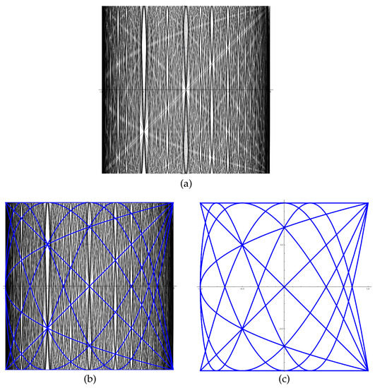
Figure 1. The first 6 white curves. Figure (a) shows the original version—the white curves are visible in the background of the plot of the first 35 Chebyshev’s polynomials. On (b) the white curves are coloured blue, on (c)—extracted.

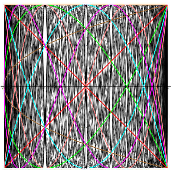
Figure 2. The first seven white curves, each in different colour.

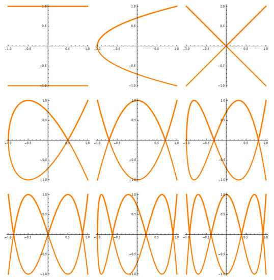
Figure 3. The first 9 white curves.

The first white curve consists of two line segments

$$\left\{\right(x,y):y=\pm 1\wedge -1\le x\le 1\}.$$

The second white curve is the following parabola

$$x=2y^2-1,y\in [-1,1].$$

The third white curve is a pair of the line segments

$$y=\pm x,x\in [-1,1].$$

The fourth white curve is Descartes’s curve

$$4x^3-3x+1=2y^2.$$

In the article of J.C. Merino [27] this curve is called Tschirnhausen’s cubic curve. Do not confuse with folium of Descartes, i.e., with the curve given by formula $x^3+y^3-3axy=0$. Descartes’s curve is a curve with a loop and has an axis of symmetry. The folium of Descartes has also an asymptote—see more in ([28] Subsection 3.9).

The fifth white curve is a pair of the parabolas

$$y=\pm \left(2x^2-1\right),x\in [-1,1]$$

and so on.

7. New Application—Our Expectations

We would like our application to be an answer for many different needs. We would like our application to give some tips on problems with a more complicated nature as well. As an example, let us consider positive-semi-definite polynomials factorization into the sum of squares of two polynomials of nonzero degrees. Recall that the $f\in \mathbb{R}[x_1,\dots ,x_n]$ is called positive-semi-definite if $f(x_1,\dots ,x_n)\ge 0$ for any $x_1,\dots ,x_n\in \mathbb{R}$. After rescaling variable, this problem in the case of quadratic trinomial reduces to the factorization of the following polynomial

$$x^2+2ax+b$$

where $a^2\le b$. Notice that

$$\begin{array}{cc}\hfill {\left(\cos \alpha x+\sqrt{b}\sin \beta \right)}^2+{\left(\sin \alpha x-\sqrt{b}\cos \beta \right)}^2& =x^2+2\sqrt{b}\sin (\beta -\alpha )x+b=\hfill \\ \hfill & =x^2+2ax+b,\hfill \end{array}$$

where

$$\sin (\beta -\alpha ):=\frac{a}{\sqrt{b}}.$$

It is easy to see that there exist infinitely many possibilities of realizing this factorization. For example, we have

$$\begin{array}{cc}\hfill x^2-x+1& ={\left(\cos \frac{\pi }{12}x-\sin \frac{\pi }{12}\right)}^2+{\left(\sin \frac{\pi }{12}x-\cos \frac{\pi }{12}\right)}^2=\hfill \\ \hfill & ={\left(\frac{\sqrt{2}}{2}x+\sin \frac{\pi }{12}\right)}^2+{\left(\frac{\sqrt{2}}{2}x-\cos \frac{\pi }{12}\right)}^2=\dots \hfill \end{array}$$

In the case of the higher degree polynomials, such factorization is more complex and requires the help of a computer.

Remark 3.

A first example of a positive-semi-definite polynomial of many variables which is not a sum of two or more squares of a nonzero polynomials was given by Motzkin [29], namely we have

$$M(x,y,z)=z^6+x^4{y}^2+x^2{y}^4-3x^2{y}^2{z}^2,$$

where

$$M\left(\frac{y^2}{x},\frac{x^2}{y},z\right)=F\left(x^2,y^2,z^2\right),$$

wherein F is a Cardano polynomial of a third degree

$$F(x,y,z)=x^3+y^3+z^3-3xyz=(x+y+z)\left(x+\epsilon y+{\epsilon }^{2}z\right)\left(x+{\epsilon }^{2}y+\epsilon z\right),$$

with $\epsilon :=\exp \left(i\frac{2}{3}\pi \right)$. Let us notice that positive-semi-definity of polynomial $M(x,y,z)$ follows from the inequality between arithmetic and geometric means.

Let us recall two fundamental theorems regarding the topic under consideration.

Theorem 8

(Artin, 1927). Let $f\in \mathbb{R}[x_1,\dots ,x_n]$ be a positive-semi-definite polynomial. Then f is a sum of squares of finitely many functions from the ring of rational functions $\mathbb{R}(x_1,\dots ,x_n)$.

Theorem 9

(Pfister, 1967). Let $f\in \mathbb{R}[x_1,\dots ,x_n]$ be a positive-semi-definite polynomial. Then f is a sum of squares of $2^n$ functions from the ring $\mathbb{R}(x_1,\dots ,x_n)$.

For example we have

$$M(x_1,x_2,1)=\frac{{\left(x_1^3{x}_2+x_2^3{x}_1-2x_1{x}_2\right)}^2\left(1+x_1^2+x_2^2\right)+{\left(x_1^2-x_2^2\right)}^2}{{\left(x_1^2+x_2^2\right)}^2}$$

(easy verification of this equality is left as an exercise to the Readers and Users).

More details about positive-semi-definite polynomials can be found in Olivier Benoist’s paper [30] (see also references of this paper; especially an interesting paper of Walter Rudin [31]).

Remark 4.

Cardano polynomial $F(x,y,z)$ described above is very useful in many areas of mathematics. For example, in planimetry, if $x,y,z$ are complex numbers on the complex plane, then these numbers form an equilateral triangle if and only if

$$\left(x+\epsilon y+{\epsilon }^{2}z\right)\left(x+{\epsilon }^{2}y+\epsilon z\right)=0,$$

which is equivalent to the following statement (see [32,33]).

‘the equality $F(x,y,z)=0$ holds if and only if the triangle $▵(x,y,z)$ is equilateral or its center of gravity is at 0 (in the complex plane)’.

Remark 5

(One more property of the polynomial M). In [34] it was noticed that the following polynomials

$$M_{\lambda }(x,y,z)=z^6+x^4{y}^2+x^2{y}^4-3\lambda x^2{y}^2{z}^2\mathrm{in}{\mathbb{R}}^3$$

and

$$L_{\lambda }(x,y,z,w)=w^4+x^2{y}^2+y^2{z}^2+z^2{x}^2-4\lambda xyzw\mathrm{in}{\mathbb{R}}^3,$$

which are nonnegative for any parameters $\lambda \in [0,1]$ and which cannot be described as a finite sum of squares of polynomials for any $\lambda \in (0,1]$, have one more interesting property:

• there is no set $\mathcal{M}$ of functions $\phi \in C^3$ in some neighbourhood of zero in ${\mathbb{R}}^3$ such that

  $$M_{\lambda }=\sum _{\phi \in \mathcal{M}}{\phi }^{2}insomeneighbourhoodofzeroin{\mathbb{R}}^3,$$
• there is no finite set $\mathcal{L}$ of functions $\psi \in C^3$ in some neighbourhood of zero in ${\mathbb{R}}^4$ such that

  $$L_{\lambda }=\sum _{\psi \in \mathcal{L}}{\psi }^{2}insomeneighbourhoodofzeroin{\mathbb{R}}^4.$$

Sketch of Proof.

Let $p\in \mathbb{R}[x_1,\dots ,x_n]$ be a homogeneous non-negative polynomial of degree $2d$ which cannot be described as a finite sum of squares of polynomials. Then this polynomial cannot be written as a finite sum of squares of functions ${\phi }_i$ of class $C^d$ in some neighbourhood of zero in ${\mathbb{R}}^n$. Otherwise, based on Taylor’s formula, each ${\phi }_i$ could be written in the following form ${\phi }_i=q_i+o\left({\left|x\right|}^d\right)$ where $q_i$ are a homogeneous polynomials of degree d. It would imply that p is a finite sum of squares of such polynomials $q_i$ in some neighbourhood of zero in ${\mathbb{R}}^n$, a contradiction. □

Remark 6.

An important area of applications of the positive polynomials is differential equations [35,36]. One of basic problems in this topic that still remains open is ‘how to determine the positivity of higher-order multivariate polynomials, which is a further problem of Hilbert’s 17th problem?’ [36,37]. W. X. Ma and Y. Zhou proved in ([36] Theorem 3.2) that if a quadratic function f is positive on ${\mathbb{R}}^M$, i.e., $f\left(x\right)>0$ for all $x\in {\mathbb{R}}^M$, then there is a positive constant d such that $f\left(x\right)\ge d$ for all $x\in {\mathbb{R}}^M$. It is quite surprising but this fact is not true for higher-order multivariate polynomials. Indeed, consider the following counterexamples:

$$\begin{array}{cc}\hfill f_{m,n}(x,y)& =x^{2m}+{\left(x^n{y}^n-1\right)}^2,m,n\in \mathbb{N},\hfill \\ \hfill g_{k,m,n}(x,y)& =\left(y^{2n}+{(y+1)}^{2n}\right)x^{2m}+{\left(x^k{y}^k-1\right)}^2,k,m,n\in \mathbb{N},m>n\hfill \end{array}$$

for which we have

$$f_{m,n}(x,y)>0$$

since $f_{m,n}(0,y)=1$ and $f_{m,n}(x,y)\ge x^{2m}>0$ whenever $x\ne 0$, and

$$g_{k,m,n}(x,y)>0$$

since $g_{k,m,n}(0,y)=1$ and $g_{k,m,n}(x,y)\ge \left(y^{2n}+{(y+1)}^{2n}\right)x^{2m}>0$ whenever $x\ne 0$.

Moreover we have:

$$\underset{r\to \infty }{\lim }{f}_{m,n}\left(r^{-1},r\right)=\underset{r\to \infty }{\lim }g\left(r^{-1},r\right)=0.$$

This implies immediately that both $f_{m,n}$ and $g_{k,m,n}$ cannot be bounded from below by any positive constant.

8. Final Remark

Let us go back to our expectations. We hope that our readers (and future users) will actively support us and that we will able to develop our application to include more detailed information which we have not considered yet.

We are very grateful for all remarks made by referees which allowed us to improve the presentation of this article. Thanks to them we supplemented our paper with Remark 6 above and Formula (6).

References

- Dubickas, A.; Hare, K.G.; Jankauskas, J. There are no two non-real conjugates of a Pisot number with the same imaginary part. Math. Comput. 2017, 86, 935–950. [Google Scholar] [CrossRef]
- Mostowski, A.; Stark, M. Introduction to Higher Algebra; PWN: Warsaw, Poland, 1972. [Google Scholar]
- Auckly, D. Solving the Quartic with a pencil. Am. Math. Mon. 2007, 114, 29–39. [Google Scholar] [CrossRef]
- Delone, B.N. Algebra (Theory of algebraic equations). In Mathematics, Its Subject, Methods and Significance, Part I; Academy of Science Press: Moscow, Russia, 1956. (In Russian) [Google Scholar]
- Stewart, I. Cooking the Classics. Math. Intell. 2011, 33, 61–71. [Google Scholar] [CrossRef]
- Olver, F.W.I.; Lozier, D.W.; Boisvert, R.F.; Clark, C.W. NIST Handbook of Mathematical Functions; Cambridge University Press: Cambridge, UK, 2010. [Google Scholar]
- Dubickas, A.; Jankauskas, J. Linear relations with conjugates of a Salem number. J. Théorie Nombres Bordx. 2020, 32, 179–191. [Google Scholar] [CrossRef]
- Spearman, B.K.; Williams, K.S. Characterization of solvable quintics x5 + ax + b. Am. Math. Mon. 1994, 101, 986–992. [Google Scholar] [CrossRef]
- Spearman, B.K.; Williams, K.S. On solvable quintics x5 + ax + b and x5 + ax2 + b. Rocky Mt. J. Math. 1996, 26, 753–772. [Google Scholar] [CrossRef]
- Spearman, B.K.; Williams, K.S. The factorization of x5 ± xa + n. Fibonacci Q. 1998, 36, 158–170. [Google Scholar]
- Johnstone, J.A.; Spearman, B.K. On a sequence of nonsolvable quintic polynomials. J. Integer Seq. 2009, 12, 3. [Google Scholar]
- Adamchik, V.; Trott, M.; Bonadies, J.; Lofgren, J.; Beck, G.; Gray, T.; Buck, J.; Ice, D.; Wolfram, S. Solving the Quintic with Mathematica—Poster; Wolfram Research Inc.: Champaign, IL, USA, 1995. [Google Scholar]
- Berndt, B.C.; Spearman, B.K.; Williams, K.S. Commentary on an unpublished lecture by G.N. Watson on solving the quintic. Math. Intell. 2002, 24, 15–33. [Google Scholar] [CrossRef]
- Bremner, A.; Ulas, M. On the reducibility type of trinomials. Acta Arith. 2012, 153, 349–372. [Google Scholar] [CrossRef][Green Version]
- Bremner, A. On trinomials of type xn + Axm + 1. Math. Scand. 1981, 49, 145–155. [Google Scholar] [CrossRef]
- Schinzel, A. On Reducible Trinomials. Available online: http://pldml.icm.edu.pl/pldml/element/bwmeta1.element.zamlynska-aa3b2a30-9a73-456e-be32-024a741a26ec/c/rm32901.pdf (accessed on 16 December 2020).
- Alekseev, V.M. (red.) Selected Problems from ‘American Mathematical Monthly’; Mir: Moscow, Russia, 1977. (In Russian) [Google Scholar]
- Drungilas, P.; Jankauskas, J.; Junevičius, G.; Klebonas, L.; Šiurys, J. On certain multiples of Littlewood and Newman polynomials. Bull. Korean Math. Soc. 2018, 58, 1491–1501. [Google Scholar]
- Baradaran, J.; Taghavi, M. Polynomials with coefficients from a finite set. Math. Slovaca 2014, 64, 1397–1408. [Google Scholar] [CrossRef][Green Version]
- Länger, H. On the dynamic behaviour of Chebyshev polynomials. Elemente der Mathematik 1995, 50, 28–30. [Google Scholar]
- Paszkowski, S. Numerical Applications of Chebyshev’s Polynomials and Series; PWN: Warsaw, Poland, 1975. (In Polish) [Google Scholar]
- Piessens, R. Computing integral transforms and solving integral equations using Chebyshev polynomial approximations. J. Comp. Appl. Math. 2000, 121, 113–124. [Google Scholar] [CrossRef]
- Rivlin, T. Chebyshev Polynomial from Approximation Theory to Algebra and Number Theory, 2nd ed.; Wiley: New York, NY, USA, 1990. [Google Scholar]
- Mason, J.C.; Handscomb, D.C. Chebyshev Polynomials; Chapman & Hall/CRC: Boca Raton, FL, USA, 2003. [Google Scholar]
- Prudnikov, A.P.; Bryczkov, A.J.; Mariczev, O.I. Integrals and Series, Elementary Functions; Nauka: Moscow, Russia, 1981. (In Russian) [Google Scholar]
- Ortiz, E.L.; Rivlin, T.J. Another look at the Chebyshev polynomials. Am. Math. Mon. 1983, 90, 3–11. [Google Scholar] [CrossRef]
- Merino, J.C. Lissajous Figures and Chebyshev Polynomials. Coll. Math. J. 2003, 34, 122–127. [Google Scholar] [CrossRef]
- Niczyporowicz, E. Plane Curves—Selected Topics in Analytic and Differential Geometry; PWN: Warsaw, Poland, 1991. (In Polish) [Google Scholar]
- Motzkin, T.S. The arithmetic-geometric inequality. In 1967 Inequalities (Proc. Sympos. Wright-Patterson Air Force Base, Ohio, 1965); Academic Press: New York, NY, USA, 1967; pp. 205–224. [Google Scholar]
- Benoist, O. Writing positive polynomials as sums of (few) squares. EMS Newsl. 2017, 8–13. [Google Scholar] [CrossRef]
- Rudin, W. Sums of squares of polynomials. Am. Math. Mon. 2000, 107, 813–821. [Google Scholar] [CrossRef]
- Abu-Saymeh, S.; Hajja, M. Equicevian points on the altitudes of a triangles. Elem. Math. 2012, 67, 187–195. [Google Scholar] [CrossRef]
- Wituła, R. Complex Numbers, Polynomials and Partial Fraction Decomposition Part 1, 2 and 3; Silesian University of Technology Press: Gliwice, Poland, 2010. (In Polish) [Google Scholar]
- Bony, J.-M.; Broglia, F.; Colombini, F.; Pernazza, L. Nonnegative functions as squares or sums of squares. J. Funct. Anal. 2006, 232, 137–147. [Google Scholar] [CrossRef][Green Version]
- Ma, W.-X.; Zhang, Y.; Tang, Y. Symbolic Computation of Lump Solutions to a Combined Equation Involving Three Types of Nonlinear Terms. East Asian J. Appl. Math. 2020, 10, 732–745. [Google Scholar] [CrossRef]
- Ma, W.-X.; Zhou, Y. Lump solutions to nonlinear partial differential equations via Hirota bilinear forms. J. Differ. Equ. 2018, 264, 2633–2659. [Google Scholar] [CrossRef]
- Fernando, J.F.; Gamboa, J.M. Real Algebra from Hilbert’s 17’th Problem. Available online: http://www.mat.ucm.es/~josefer/articulos/rgh17.pdf (accessed on 16 December 2020).
Publisher’s Note: MDPI stays neutral with regard to jurisdictional claims in published maps and institutional affiliations. |
© 2020 by the authors. Licensee MDPI, Basel, Switzerland. This article is an open access article distributed under the terms and conditions of the Creative Commons Attribution (CC BY) license (http://creativecommons.org/licenses/by/4.0/).