Abstract
Community search is a basic problem in graph analysis. In many applications, network nodes have certain properties that are important for the community to make sense of the application; hence, attributes are associated with nodes to capture their properties. Community influence is an important community property that can be used to rank communities in a network based on the relevance/importance of a particular attribute. Unfortunately, most of the community search algorithms introduced previously in attributed networks research work ignored the community influence. When searching for influential communities, two potential data sources can be used: network attributes and nodes. Dealing with structure-related attributes is a challenge. Recently, the graph neural network (GNN) has completely changed the field of graph representation learning by effectively learning node embedding and has achieved the most advanced results in tasks such as node classification and connection prediction. In this paper, we investigate the problem of searching for the influential communities in attributed networks. We propose an efficient algorithm for retrieving the influential communities in a large attributed network. The proposed approach contains two main steps: (1) Community detection using a graph convolutional network in a semi-supervised learning setting considering the correlation between attributes and the overall graph information, and (2) constructing the influential communities resulting from step 1. The proposed approach is evaluated on various real datasets. The experimental results show the efficiency and effectiveness of the proposed implementations.
1. Introduction
Graphs have played a critical role in big data analysis in recent years [1]. Graphs are a simple and efficient way to represent and manage information from different domains. Due to the extraordinary rise in the volume of data, it is crucial to design a method to efficiently detect hidden patterns among a group of users. A community can be defined as a set of vertices (nodes) that probably share common features, where the nodes in the same communities have more dense connections with each other than those that exist in other communities [2,3]. For example, in protein interaction networks, communities are functional modules of interacting proteins [4]; in co-authorship networks, communities correspond to scientific disciplines [5]. Two main problems have been investigated in network analysis: (1) community detection, and (2) community search. Community detection is widely used to derive a set of nodes closely interacting and having a strong relationship with each other. Detecting the strongest community among a large network (graph) has become a critical and important task in graph analysis. Different techniques for detecting communities in large networks are outlined in [2,6,7,8,9,10,11,12]. A similar problem is community search which is a query-dependent variant of the community detection problem. Community search aims to find the densely connected components that satisfy the query conditions [13]. Recently, much attention has been paid to attributed community search which aims to find query-dependent communities where the community members are closely related and have homogeneous attribute values.
Despite the studies that have been conducted to solve community detection and community search problems, previous attempts have ignored the community influence dimension. Community influence is a crucial community property that may be used to order communities in a network depending on the relevance/importance of specific attributes. Recently, detecting influential communities was studied in a few research works. It was first addressed by Li et al. in [14]; later it was investigated in [15,16,17,18]. Different community search models have been proposed based on k-core [19,20,21], k-truss [22,23,24,25], and clique or quasi-clique [26,27].
In this paper, we consider large attributed graphs where vertices are associated with attributes and propose a novel and efficient solution for finding influential communities that address the following drawbacks in the traditional community search research works:
- 1.
- A query vertex is needed as an input and then we find a group of neighboring vertices whose attributes are highly similar to those of the query vertex. The main limitation of these CS techniques is that the user has to define the query vertices. This may not be possible or appropriate for many application domains.
- 2.
- Another type of community search solution is to find related communities that share many similarities with query attributes. However, the influence (impact) of the community is not taken into account.
- 3.
- The other type of community search solution only works on non-attributed graphs and considers the influence of the community as the minimum weight of its nodes, where the weight denotes the influence (importance) of the node. However, this assumption ignores the relationship between nodes. Moreover, it fails to express the actual influence of the nodes in a community with respect to its associated attributes.
By recasting the problem of detecting communities in large graphs as a node classification problem on graphs, it can be studied from a learning perspective. Graph representation learning is the task of representing the graph or its nodes and edges by a vector space to facilitate downstream graph mining tasks [28]. In recent years, there has been a surge of interest in the development of graph neural networks (GNNs). GNNs are general deep learning architectures that can work on graph-structured data, such as data from social networks [29] or graph-based representations of molecules [30]. These properties allow you to use the GNN model to solve some complex network tasks. The basic idea of GNN is to represent the original graph as a computational graph and learn neural network primitives that generate embeddings of each node of the graph by bypassing, transforming, and aggregating node feature information throughout the graph [31]. After k aggregation iterations, a node is represented by a feature vector that has been transformed to capture the structural information of the node’s k-hop neighborhood. The representation of the original graph can be obtained through pooling, for example, by summing the vectors that represent all nodes in the graph. Different GNN solutions have been proposed with different neighborhood aggregation and graph-level pooling schemes. Then, the generated node embeddings can be used as input to any differentiable prediction layer for different tasks such as node classification [32] or link prediction [33].
In this work, we propose a semi-supervised model, named Influential Attributed Communities via Graph Convolutional Network (InfACom-GCN) which finds the top-r k-influential communities in large attributed networks. InfACom-GCN detects a tightly connected group of nodes (vertices) that dominate other nodes (vertices) in a graph for a particular domain. First, GCN is employed to decompose the graph into different partitions considering the correlation between the attributes and the overall graph information. Then, the influential communities are constructed based on these partitions. To the best of our knowledge, this is the first work that employs the GCN to find the top-r k-influential communities in attributed networks.
The rest of this paper is organized as follows: Section 2 presents the needed preliminaries and some related concepts. Section 3 presents related work. In Section 4, we discuss the influential attributed community approach. Section 5 shows the experimental results. Finally, Section 6 gives a brief summary, discusses the findings, and proposes directions for future works.
2. Preliminaries
This section presents some related concepts that will be used in the rest of this paper. Graph neural network is discussed in Section 2.1. Section 2.2 presents a different level of the graph-based task. Finally, in Section 2.3, the graph-based learning methods are introduced.
2.1. Graph Neural Networks
Graph Neural Network (GNN) is a deep learning-based method that extends the existing neural network methods to process data represented in the graph domain [31,34,35,36,37,38,39,40]. The node features and the graph structure are used by GNNs to learn a vector representation of a node, , or the entire graph, . GNNs follow a neighborhood aggregation strategy in which the representation of a node is iteratively updated by aggregating representations of its neighbors. After k aggregation iterations, the node’s representation captures structural information within its neighborhood of the k-hop network. Officially, the layer k of a GNN is:
where is the vector that contains features of node v at layer k, , and is a set of nodes adjacent to v. There are different architectures that have been proposed for AGGREGATE. In node classification, the node representation of the last iteration is employed for prediction. In graph classification, the READOUT function is responsible for aggregating all node features from the last iteration to obtain the entire graph’s representation :
where READOUT can be a simple permutation invariant function, such as a summation or a more complex graph-level pooling function.
2.2. Classification of Graph-Based Tasks
Graph-based data has knowledge embedded at various levels of the structure. At the node level, different node-based tasks are defined. Moreover, edge-level tasks are defined. In addition, graph-level tasks that cover the entire graph or subgraphs are also defined according to different applications.
- 1.
- Node-level task. This focuses on tasks such as node classification, node clustering, and node regression. Node classification classifies nodes into different groups, whereas the node regression task predicts an accurate value for each node. Node clustering is used to divide a node into different classes and group-related nodes. An example of a node-level task is the problem of protein folding. In this problem, amino acids in a protein sequence are treated as nodes and the proximity between amino acids as the edges. Using convolutional GNNs can extract high-level node representations.
- 2.
- Edge-level task: Edge classification and link prediction are considered edge-level tasks. Edge classification and link prediction are the tasks where the model needs to predict if there is an edge between two nodes or classify edge types. One important example of edge-level tasks is the recommendation system where items and users represent the nodes and user–item interactions represent the edges. The biomedical graph link prediction is another example where drugs and proteins represent the nodes, and the interactions between them represent the edges. The task is to find out what is the probability that Simvastatin and Ciprofloxacin will break down muscle tissue. It uses the hidden representation of the two nodes of the GNN as input and uses the similarity function to determine the connection strength of the edges.
- 3.
- Graph-level task: Graph-level representation is required for graph classification, regression, and matching tasks to be modeled. Drug discovery is an example of a graph-level task; atoms represent nodes and chemical bonds between them represent edges. Physics simulation is another example of graph-based tasks where particles can be represented as nodes and interaction between particles can be represented as edges. Moreover, subgraph-level tasks are considered. Traffic prediction is an example of subgraph-level tasks considering the road network as a graph; road segments represent the nodes and connectivity between road segments as the edges. GNNs are often combined with pooling and readout operations to obtain a compact representation on the graph level.
2.3. Graph-Based Learning Methods
The graph-based learning methods are divided into different training settings from the perspective of supervision: (1) supervised learning, (2) unsupervised learning, and (3) semi-supervised learning [41]. Supervised learning is a machine learning task that learns a function that maps an input to an output based on sample input–output pairs [42]. It uses the labeled data to train the model to accurately predict data that has never been seen before such as classification and regression. Unsupervised learning analyzes unlabeled datasets without human intervention [42]. It is often used to extract common features, identify meaningful trends and structures, and group them into results for exploratory purposes. The most common unsupervised learning tasks are feature learning, clustering, density estimation, dimensionality reduction, anomaly detection, and finding association rules. Semi-supervised learning can be defined as a hybrid of both supervised and unsupervised methods. It operates on both labeled and unlabeled data [42]. Therefore, it lies between unsupervised learning and supervised learning. In the real world, labeled data are rare in several contexts, and unlabeled data are common, where semi-supervised learning is useful [41,43]. The goal of the semi-supervised learning model is to provide a better output for prediction than those generated using only the model’s labeled data.
3. Related Work
This paper classifies the related work into the following two main categories: influential community search, and community detection with graph neural networks.
3.1. Influential Community Search
The problem of identifying the most influential communities was first formulated by Li et al. [14]. A formal definition of the influence of an individual (node) and a community was developed. An index called the ICP Index has also been proposed to speed up search algorithms for influential communities. It supports efficient searching of top-r k-influential communities in optimal time. The ICP Index is based on the inclusion relationship form of the k-influential communities. Based on such an inclusion relationship, all the k-influential communities can be organized using a tree-shape (or a forest-shape) structure. In [18], a new community model was proposed that reveals the communities with the highest outer influences. Moreover, a tree-based index structure and different algorithms were developed to improve the search performance. In [15], an instance optimization algorithm was proposed to retrieve the top-k influential communities without using an index. The authors in [44], propose a new Skyline community model that recognizes the community in a multivalued network where each node has d numeric attributes. Finally, the authors in [45] discussed the major factors that affect the influence of the community. Moreover, they proposed two techniques for retrieving the top-r k-influential communities one for sequential implementation with three variations and one for parallel implementation.
3.2. Community Detection via GNN
In recent years, various models of graph neural network (GNN) have been proposed [46,47,48,49,50]. The authors in [47] introduced a special neural network approach suitable for learning network communities and node semantics at the same time. This approach is based on GCN for unsupervised community detection in attribute networks and is called GUCD. GUCD consists of three main parts: (1) the encoder which contains three convolutional layers, where the first two layers were to learn a deep representation of the attribute network, and the third layer was to model and derive node community membership using both the deep representation and network information, (2) a dual decoder which uses the derived communities to separately reconstruct network topology and node attributes, and (3) a local enhancement part that utilizes local information to enhance communities from a local view. Moreover, the authors in [48] proposed a new approach for solving community detection problems in a supervised learning setting based on GNNs. A change to the GNN architecture is proposed to expose edge adjacency information by including a non-backtracking operator for graphs. This operator is defined through the edges of the graph, allowing a directed flow of information even when the original graph is undirected. In [49], the authors proposed a new community detection algorithm called Self-Expressive Community detection in a graph (SEComm). SEComm combined the principle of self-expressiveness with the framework of a self-supervised graph neural network and generates node communities from the embeddings obtained. In [50], the authors introduced a high-order graph convolution approach for obtaining smooth node embeddings that represent the global cluster structure. Then, spectral clustering uses node embeddings to detect communities. Finally, the authors in [46] proposed the Query-Driven Graph Convolutional Networks (QD-GCN) framework. QD-GCN is used for finding query-dependent communities with cohesive structure and homogeneous attributes w.r.t. the query vertices and query attributes.
4. Influential Attributed Communities via Graph Convolutional Network (InfACom-GCN)
In this section, we propose a new approach that finds top-r k-influential communities for a specific attribute(s). Figure 1 shows the architecture of the – approach. This approach contains two main steps: (1) Community detection using GCN [51] in a semi-supervised learning setting, and (2) constructing the top-r k-influential communities from the partitions that result from step 1.
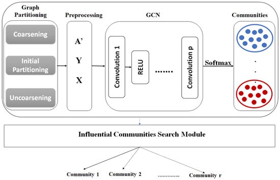
Figure 1.
InfACom-GCN architecture.
4.1. Community Detection Using GCN
Consider an undirected attributed network G = (A, X), where A is an adjacency matrix of n nodes and X is an attribute matrix of m attributes per node. The network G is partially labeled. The communities of some nodes are known, and are indexed by a set of k labels . The problem of semi-supervised community detection is then to label the remaining unlabeled nodes in G, and as a result form k communities of nodes.
This section aims to use GCN to decompose the given graph into different partitions such that the final partitions should satisfy two properties: (1) Topology similarity: Nodes that belong to the same community have more connections to each other than nodes outside the community. (2) Attribute homogeneity: Nodes whose attribute vectors are close to each other are most likely assigned to the same community.
In GCN, the graph convolution operator needs to propagate embeddings using the interactions between nodes in the graph. The classification loss on a single node depends on a huge number of other nodes. Due to this node dependence, backpropagation needs to store all the embeddings, which makes the training of GCN very slow and require lots of memory. The current algorithms have two problems: (1) high computational cost where the cost increases exponentially with the number of GCN layers, and (2) large space requirements to keep the whole graph and embeddings of each node of the graph in memory. In order to overcome these problems and avoid heavy neighborhood searches, there is a need to divide the original graph into different partitions and focus on the neighbors within each partition.
4.1.1. Graph Partitioning
The idea is that neighboring nodes with similar feature representations tend to be in the same partition. In this section, the goal is to divide the graph into subgraphs with the lowest number of edges that cross partitions (edge-cut). The multilevel graph partitioning paradigm in [52] is employed. In this paper, the multilevel k-way partitioning algorithm is employed to partition the graph into different subgraphs to ensure the number of edges between vertices in distinct partitions is kept to a minimum.
Given an undirected graph , . G is decomposed into k partitions {} such that for , , , and the number of edges that link between nodes in different partitions (edge-cut) is minimized. The algorithm for partitioning the graph contains three main phases:
- 1.
- Graph coarsening: In this phase, a sequence of smaller graphs such that is constructed. Each graph is constructed from the preceding graph by collapsing together a maximal size set of adjacent pairs of vertices and a multinode consisting of these vertices is created. This process continues until the size of the graph has been decreased to just a few hundred vertices.Let be the set of vertices of combined to form vertex s of . The weight of the vertex s is equal to the sum of the weights of all vertices in . The edges of s are the union of all edges of the vertices in . The idea of edge collapse can be formally defined in terms of matching. Graph matching is a set of edges where no two edges share the same vertex. Discovering a matching of and reducing the vertices being matched into multinodes produces a coarser next-level graph from . The match must be maximal because the purpose of the vertex match is to reduce the size of the graph . Matching is called maximal if there are no more edges that can be added. In this paper, the heavy-edge matching in [53] is used which finds a maximal matching that contains edges with large weight.
- 2.
- Initial partitioning: In this phase, k-way partitioning of the coarse graph is computed such that each partition contains roughly vertex weight of the original graph. The weights of the vertices and edges of the coarser graph can be used to apply the balanced partitioning and the minimum edge-cut.
- 3.
- Uncoarsening: the partitioning of the smallest graph is projected to larger graphs by assigning the pairs of vertices that were collapsed together to the same partition. The vertices are frequently transferred between partitions after each projection step to increase the partitioning solution’s quality.
Finally, the adjacent matrix of each subgraph is obtained.
4.1.2. The Graph Convolution Network
GCN uses the graph convolution operation to obtain the node embeddings layer by layer. At each layer, node embedding is obtained by collecting the embeddings of its neighbors, followed by one or a series of layers of linear transformations and nonlinear activations. The last layer embedding is then used for some end tasks. In the node classification problem, the last layer embedding is passed to a classifier to predict node labels, so GCN parameters can be trained end to end.
Consider a graph , where V represents the set of n vertices, E represents the set of edges, and A is the adjacency matrix with (i, j) entry equaling 1 if there is an edge between vertices and and 0 otherwise. is the feature matrix of all nodes where f is the number of features. A multi-layer Graph Convolutional Network (GCN) [32] is considered with the following layer-wise propagation rule:
where is the embedding at the l-th layer for all the n nodes, is the adjacency matrix of G with self-connections where I is the identity matrix, is the degree matrix where , W is the trainable weight matrix, and is the activation function, such as the ReLU.
The node classification assumes that each node is associated with a label , and the goal of the graph representation learning for it is to learn a representation vector such that s label can be predicted as . Then, the fully connected neural network takes the node representation from the final layer as its input and makes label predictions. Semi-supervised node classification evaluates the training loss function of all labeled nodes, assuming that only a small portion of the nodes in the graph have label information. The goal is to learn the weight matrix by minimizing the loss function:
where contains all the labels for the labeled nodes; is the i-th row of with the ground-truth label denoting the predicted final layer of node i.
The partitioning technique is used, and we only pay attention to the neighbors inside each partition in order to avoid conducting a thorough neighborhood search. By applying the partition module on G, the original graph G is decomposed into p partitions such that , where is the set of nodes in the i-th partition, and is the set of edges between nodes in . Moreover, the links between partitions are removed and the adjacency matrix A is changed by △ where . In addition, the feature matrix X and labels Y should be partitioned into and corresponding to the new subgraph where and are features and labels of the nodes of , respectively. As a result, the final embedding matrix’s i-th row is as follows [51],
Usually, each node and its neighbors exist in the same partition, so all nodes of the same partition are put in the same batch. Consequently, there is a need to store only the node embeddings within the current batch. To reduce the error, the links between partitions should be minimal.
Training the model: As semi-supervised classification is used, the dataset is split into training, validation, and test. We use a random distribution of training, validation, and test sets. The GCN model uses the non-linear activation function ReLU [54] for the propagation rule. The ReLU function is applied row-wise on the last layer in the GCN. The cross-entropy loss is performed on known node labels. The loss is backpropagated and the weight matrices are updated in each layer. The model is trained with a specified number of epochs where the loss is calculated at each training instance and the error is backpropagated. The Adam optimizer [55] was used to fully train the model. Details are given in Algorithm 1.
| Algorithm 1: GCN based on graph partitioning. |
 |
4.1.3. Influential Community Construction
This section aims to retrieve the influential communities from the communities detected in the previous step and introduces how to construct communities from the space. The influential community is defined as a closely connected group of vertices having some dominance over other groups of vertices with the expertise (a set of keywords) matching with the query terms.
The main idea is to group data points together that have high density [56] given the radius of the area and the minimum number of data points required to form a dense region. Low-density regions are called outliers.
R and k represent the radius of the region and the minimum number of data points to consider. First, the algorithm starts by randomly selecting a point (P) from the data points and finding all adjacent points within its radius R. If the number of adjacent points is k or more, P is considered as a core point and P forms the first community with its neighbors. After creating the first community, all its members are checked to see if they can find their neighbors in R. If a member has at least k neighbors, the first community is expanded by adding those neighbors to the community. This process continues until no more points could be added to that community. When this point is reached, a new community is initiated for a unvisited point that has not been assigned to a community yet. Then, for each point, find and assign all connected points recursively. Iterate through all unvisited points from the data points and assign them to the closest community at distance R. If any point does not match any available community, assign it as an outlier point.
Details are given in Algorithm 2, which is described below.
For each point P, the algorithm finds its community members by returning its neighbors within region R (step 3). Then, it checks that the size of the community members should be ≥k (the density condition). If the condition is satisfied, each community member receives a community ID and P is marked as visited and removed from the points (steps 5–9). Otherwise, P is assigned as an outlier. Next, the algorithm tries to extend the generated community by checking each member of the generated community and its neighbors within a region R (steps 11–20). This process is repeated until all members are examined. After all points acquire a community ID, each group of members with the same ID is returned as an influential community (steps 29 to 33).
| Algorithm 2: Influential Communities Construction. |
 |
5. Experimental Evaluation
This section presents the experimental results that measure the efficiency of our proposed implementations. The proposed algorithms are implemented in Python and all experiments are conducted on Windows 10 with Intel(R) Core(TM) i7 CPU and 16 GB RAM.
5.1. Datasets
Experimental studies are conducted on real datasets illustrated in Table 1. Datasets were downloaded from (https://linqs.soe.ucsc.edu/data (accessed on 16 March 2022)). Three benchmark datasets for citation networks are used: Citeseer, Cora, and PubMedDiabetes. Citeseer is a citation network containing 4660 edges and 3312 nodes which are classified into six classes. Each node is represented by 3703-dimensional node features. Cora is a citation network which contains 5429 edges and 2708 nodes classified into seven classes. Each node is represented by a 1433-dimensional word vector known as a node feature. PubMedDiabetes is a dataset containing 44,338 edges and 19,717 nodes classified into three classes. Each node is represented by a TF/IDF weighted word vector from a dictionary which consists of 500 unique words.

Table 1.
Dataset description.
5.2. Result Analysis
In this section, we demonstrate and discuss the results of the experiments. Section 5.2.1 shows the impact of model hyperparameters on the performance of –. Section 5.2.2 introduces a comparison between – and the state-of-the-art methods. Finally, Section 5.2.3 introduces the accuracy of – with more layers.
5.2.1. Analysis of the Impact of Model Hyperparameters on the Performance
- (A)
- Learning rate: Figure 2 shows the change in accuracy with the learning rate for different types of networks. The best accuracy is achieved with the smaller learning rate of 0.01. The learning rate has been increased up to 0.1. However, we note that with the increase in the learning rate, the accuracy drops a lot.
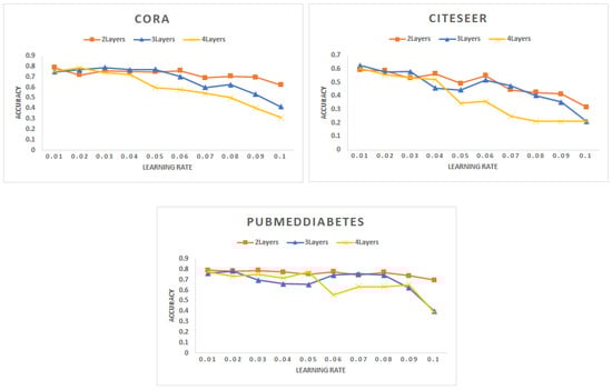 Figure 2. Accuracy for different networks varying the learning rate with a different number of layers.
 - (B)
- Dropout: Figure 3 shows the accuracy (F1 score) for different datasets. In this experiment, we vary the dropout rate to determine the optimized parameter with maximum accuracy where all datasets are decomposed into 10 partitions and each batch contains 2 partitions. We noticed that the accuracy decreases with the increase of the dropout for all datasets. This result is aligned with the results mentioned in [57].
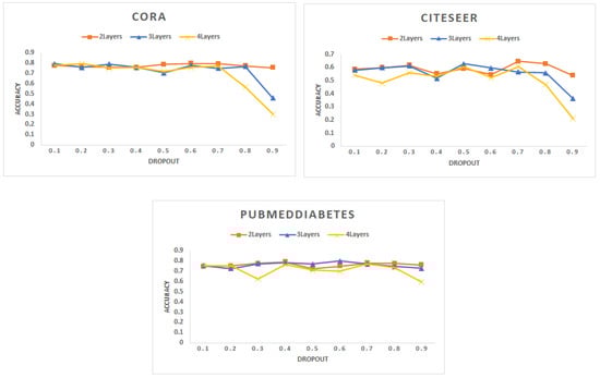 Figure 3. Accuracy for different networks varying the dropout hyperparameter with a different number of layers.
 - (C)
- Number of Epochs: Figure 4 shows the accuracy (F1 score) for different datasets with 2, 3, and 4 layers of graph convolutional network. The rate of dropout for the input of each GCN layer is 50%. Each dataset is decomposed into 10 partitions, where each batch contains 2 partitions.
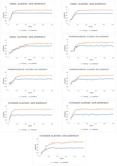 Figure 4. Accuracy for different networks varying the number of epochs with a different number of layers.
5.2.2. Comparison with State-of-the-Art Methods
To ensure the efficiency of – for retrieving the influential communities, we compared the proposed algorithm with – in [32], in [58], and in [59]. – presents the semi-supervised train paradigm and generalizes the convolutional operation on graph data which needs to store all node embeddings. extends the convolutional operation of GCN to mean, max pooling, and LSTM aggregator and introduces a sampling strategy before employing convolutional operations on neighbor nodes. It is designed to take advantage of node attribute information to efficiently generate representations of evolving graphs using previously unseen data. uses a fixed-size set of neighbors during backpropagation through layers. is a full batch model that uses a self-attention mechanism to learn the weights between each pair of connected nodes, allowing self-attention to discover the most representative parts of the input. The proposed algorithm is compared with the state-of-the-art approaches in terms of memory usage, time costs, and accuracy (F1 score):
- (A)
- Memory Usage: Table 2, Table 3 and Table 4 show the memory usage of each algorithm in megabytes for different datasets with 2, 3, and 4 layers (the number of hidden units is 128). The results show that all previous algorithms need much more memory for training than InfACom-GCN. This is because the InfACom-GCN does not keep the full graph and embeddings of each node of the graph in memory, it just needs to store only the node embeddings within the current batch. On the other hand, and are full batch models that require storing all the intermediate embeddings to compute the full gradient which leads to consuming more memory.
Table 2. Memory usage in megabytes for Cora dataset using different numbers of layers (the number of hidden units is 128).
Table 3. Memory usage in megabytes for Citeseer dataset using different numbers of layers (the number of hidden units is 128).
Table 4. Memory usage in megabytes for PubMedDiabetes dataset using different numbers of layers (the number of hidden units is 128).
- (B)
- Time cost: Table 5, Table 6 and Table 7 show the average of the training time of , –, –, and for Cora, Citeseer, and PubMedDiabetes, respectively, using different numbers of layers (the number of hidden units is 128). All results show that – outperforms all other algorithms. This is because – avoids the high computational cost where the loss on a single node depends only on the node embeddings within the current batch. On the other hand, the full batch is particularly slow since it performs calculations on the entire training set at each step. As a result, doing so becomes extremely computationally costly.
Table 5. Average time of 50 epochs for Cora dataset using 2, 3, and 4 layers (the number of hidden units is 128).
Table 6. Average time of 50 epochs for Citeseer dataset using 2, 3, and 4 layers (the number of hidden units is 128).
Table 7. Average time of 50 epochs for PubMedDiabetes dataset using 2, 3, and 4 layers (the number of hidden units is 128).
- (C)
- Accuracy (F1 score): Table 8, Table 9 and Table 10 show the accuracy (F1 score) of , , –, and – for Cora, Citeseer, and PubMedDiabetes, respectively. The results show that the accuracy of all algorithms is similar, indicating that the accuracy is not adversely affected by the original graph’s partitioning.
Table 8. Average accuracy of 50 epochs for Cora dataset using 2, 3, and 4 layers (the number of hidden units is 128).
Table 9. Average accuracy of 50 epochs for Citeseer dataset using 2, 3, and 4 layers (the number of hidden units is 128).
Table 10. Average accuracy of 50 epochs for PubMedDiabetes dataset using 2, 3, and 4 layers (the number of hidden units is 128).
5.2.3. Deep Neural Networks
Table 11 shows the test accuracy (F1 score) with different numbers of layers (the number of hidden units is 128). For the dataset, the empirical results show that after using 10 layers, – has a dramatic loss of accuracy. For the dataset, the empirical results show that after using 8 layers, – has a significant loss in accuracy. For the dataset, the empirical results show that after using 9 layers, – has a significant loss in accuracy. This is because nodes will have access to information from nodes that are far and may not be similar to them, which makes all node embeddings similar (over-smoothing). The trial and error method is used to determine the optimal value of the number of layers.
Table 11.
The test accuracy (F1 score) of – using different numbers of layers.
6. Conclusions and Future Work
The problem of community search over very large graphs is a fundamental problem in graph analysis. However, certain applications require finding the top-r influential communities in the network. This paper introduced a semi-supervised model, named Influential Attributed Communities via Graph Convolutional Network (InfACom-GCN) which finds the top-r k-influential communities in large attributed networks. First, GCN is employed to decompose the graph into different partitions considering the correlation between attributes and the overall graph. Then, the top-r k-influential communities are constructed from the resulting communities. The proposed algorithms are evaluated on various real datasets. The experimental results show the efficiency and effectiveness of the proposed implementations. For future work, we will study how to use an attention neural network to find the influential communities in an attributed graph from only one step. Finally, the logical operations (AND–OR) that are used for conjoining the query terms should be considered.
Author Contributions
Conceptualization, N.A.H., H.M.O.M. and M.E.E.-S.; formal analysis, N.A.H., H.M.O.M. and M.E.E.-S.; funding acquisition, H.M.O.M.; investigation, N.A.H.; methodology, N.A.H., H.M.O.M. and M.E.E.-S.; project administration, H.M.O.M. and M.E.E.-S.; resources, N.A.H.; supervision, H.M.O.M. and M.E.E.-S.; validation, N.A.H.; visualization, N.A.H.; writing—original draft, N.A.H.; writing—review and editing, N.A.H., H.M.O.M. and M.E.E.-S. All authors have read and agreed to the published version of the manuscript.
Funding
This research received no external funding.
Institutional Review Board Statement
Not applicable.
Informed Consent Statement
Not applicable.
Data Availability Statement
Data is contained within the article.
Conflicts of Interest
The authors declare no conflict of interest.
References
- Cai, H.; Zheng, V.W.; Chang, K.C. A Comprehensive Survey of Graph Embedding: Problems, Techniques and Applications. arXiv 2017, arXiv:1709.07604. [Google Scholar] [CrossRef]
- Fortunato, S. Community detection in graphs. Phys. Rep. 2010, 486, 75–174. [Google Scholar] [CrossRef]
- Huang, X.; Lakshmanan, L.V.; Xu, J. Community Search over Big Graphs: Models, Algorithms, and Opportunities. In Proceedings of the 2017 IEEE 33rd International Conference on Data Engineering (ICDE), San Diego, CA, USA, 19–22 April 2017; pp. 1451–1454. [Google Scholar]
- Jonsson, P.F.; Bates, P.A. Global topological features of cancer proteins in the human interactome. Bioinformatics 2006, 22, 2291–2297. Available online: http://xxx.lanl.gov/abs/https://academic.oup.com/bioinformatics/article-pdf/22/18/2291/16851721/btl390.pdf (accessed on 1 January 2022). [CrossRef]
- Zhou, Y.; Cheng, H.; Yu, J.X. Graph Clustering Based on Structural/Attribute Similarities. Proc. VLDB Endow. 2009, 2, 718–729. [Google Scholar] [CrossRef]
- Wu, Y.; Jin, R.; Li, J.; Zhang, X. Robust Local Community Detection: On Free Rider Effect and Its Elimination. Proc. VLDB Endow. 2015, 8, 798–809. [Google Scholar] [CrossRef]
- Sariyüce, A.E.; Seshadhri, C.; Pinar, A. Local Algorithms for Hierarchical Dense Subgraph Discovery. Proc. VLDB Endow. 2018, 12, 43–56. [Google Scholar] [CrossRef]
- Shao, J.; Han, Z.; Yang, Q.; Zhou, T. Community Detection Based on Distance Dynamics. In Proceedings of the 21th ACM SIGKDD International Conference on Knowledge Discovery and Data Mining, Sydney, Australia, 10–13 August 2015; Association for Computing Machinery: New York, NY, USA, 2015; pp. 1075–1084. [Google Scholar]
- Chang, L.; Li, W.; Lin, X.; Qin, L.; Zhang, W. pSCAN: Fast and exact structural graph clustering. In Proceedings of the 2016 IEEE 32nd International Conference on Data Engineering (ICDE), Helsinki, Finland, 16–20 May 2016; pp. 253–264. [Google Scholar]
- Jagadishwari, V.; Umadevi, V. Empirical analysis of community detection algorithms. In Proceedings of the 2017 Second International Conference on Electrical, Computer and Communication Technologies (ICECCT), Coimbatore, India, 22–24 February 2017; pp. 1–5. [Google Scholar]
- Varsha, K.; Patil, K.K. An Overview of Community Detection Algorithms in Social Networks. In Proceedings of the 2020 International Conference on Inventive Computation Technologies (ICICT), Coimbatore, India, 26–28 February 2020; pp. 121–126. [Google Scholar]
- Farzad, B.; Pichugina, O.; Koliechkina, L. Multi-Layer Community Detection. In Proceedings of the 2018 International Conference on Control, Artificial Intelligence, Robotics Optimization (ICCAIRO), Prague, Czech Republic, 19–21 May 2018; pp. 133–140. [Google Scholar]
- Sozio, M.; Gionis, A. The Community-search Problem and How to Plan a Successful Cocktail Party. In Proceedings of the Proceedings of the 16th ACM SIGKDD International Conference on Knowledge Discovery and Data Mining, Washington, DC, USA, 25–28 July 2010; ACM: New York, NY, USA, 2010; pp. 939–948. [Google Scholar]
- Li, R.H.; Qin, L.; Yu, J.X.; Mao, R. Influential Community Search in Large Networks. Proc. VLDB Endow. 2015, 8, 509–520. [Google Scholar] [CrossRef]
- Bi, F.; Chang, L.; Lin, X.; Zhang, W. An Optimal and Progressive Approach to Online Search of Top-k Influential Communities. Proc. VLDB Endow. 2018, 11, 1056–1068. [Google Scholar] [CrossRef]
- Chen, S.; Wei, R.; Popova, D.; Thomo, A. Efficient Computation of Importance Based Communities in Web-Scale Networks Using a Single Machine. In Proceedings of the 25th ACM International on Conference on Information and Knowledge Management, Indianapolis, IN, USA, 24–28 October 2016; ACM: New York, NY, USA, 2016; pp. 1553–1562. [Google Scholar]
- Li, R.H.; Qin, L.; Yu, J.X.; Mao, R. Finding Influential Communities in Massive Networks. VLDB J. 2017, 26, 751–776. [Google Scholar] [CrossRef]
- Li, J.; Wang, X.; Deng, K.; Yang, X.; Sellis, T.; Yu, J.X. Most Influential Community Search over Large Social Networks. In Proceedings of the 2017 IEEE 33rd International Conference on Data Engineering (ICDE), San Diego, CA, USA, 19–22 April 2017; pp. 871–882. [Google Scholar]
- Fang, Y.; Cheng, R.; Luo, S.; Hu, J. Effective Community Search for Large Attributed Graphs. Proc. VLDB Endow. 2016, 9, 1233–1244. [Google Scholar] [CrossRef]
- Fang, Y.; Cheng, R.; Li, X.; Luo, S.; Hu, J. Effective Community Search over Large Spatial Graphs. Proc. VLDB Endow. 2017, 10, 709–720. [Google Scholar] [CrossRef]
- Zhang, F.; Zhang, Y.; Qin, L.; Zhang, W.; Lin, X. When Engagement Meets Similarity: Efficient (K,R)-core Computation on Social Networks. Proc. VLDB Endow. 2017, 10, 998–1009. [Google Scholar] [CrossRef]
- Huang, X.; Cheng, H.; Qin, L.; Tian, W.; Yu, J.X. Querying K-truss Community in Large and Dynamic Graphs. In Proceedings of the 2014 ACM SIGMOD International Conference on Management of Data, Snowbird, UT, USA, 22–27 June 2014; ACM: New York, NY, USA, 2014; pp. 1311–1322. [Google Scholar]
- Huang, X.; Lakshmanan, L.V.S.; Yu, J.X.; Cheng, H. Approximate Closest Community Search in Networks. Proc. VLDB Endow. 2015, 9, 276–287. [Google Scholar] [CrossRef]
- Huang, X.; Lakshmanan, L.V.S. Attribute-driven Community Search. Proc. VLDB Endow. 2017, 10, 949–960. [Google Scholar] [CrossRef]
- Liu, Q.; Zhao, M.; Huang, X.; Xu, J.; Gao, Y. Truss-based Community Search over Large Directed Graphs. In Proceedings of the 2020 ACM SIGMOD International Conference on Management of Data, Portland, OR, USA, 14–19 June 2020. [Google Scholar]
- Cui, W.; Xiao, Y.; Wang, H.; Lu, Y.; Wang, W. Online Search of Overlapping Communities. In Proceedings of the 2013 ACM SIGMOD International Conference on Management of Data, New York, NY, USA, 23–28 June 2013; ACM: New York, NY, USA, 2013; pp. 277–288. [Google Scholar]
- Tsourakakis, C.; Bonchi, F.; Gionis, A.; Gullo, F.; Tsiarli, M. Denser Than the Densest Subgraph: Extracting Optimal Quasi-cliques with Quality Guarantees. In Proceedings of the 19th ACM SIGKDD International Conference on Knowledge Discovery and Data Mining, Chicago, IL, USA, 11–14 August 2013; ACM: New York, NY, USA, 2013; pp. 104–112. [Google Scholar]
- Chen, F.; Wang, Y.; Wang, B.; Kuo, C.J. Graph Representation Learning: A Survey. arXiv 2019, arXiv:1909.00958. [Google Scholar] [CrossRef]
- Chen, J.; Ma, T.; Xiao, C. FastGCN: Fast Learning with Graph Convolutional Networks via Importance Sampling. arXiv 2018, arXiv:1801.10247. [Google Scholar]
- Sun, M.; Zhao, S.; Gilvary, C.; Elemento, O.; Zhou, J.; Wang, F. Graph convolutional networks for computational drug development and discovery. Briefings Bioinform. 2019, 21, 919–935. Available online: http://xxx.lanl.gov/abs/https://academic.oup.com/bib/article-pdf/21/3/919/33227266/bbz042.pdf (accessed on 1 January 2022). [CrossRef]
- Zhou, J.; Cui, G.; Zhang, Z.; Yang, C.; Liu, Z.; Sun, M. Graph Neural Networks: A Review of Methods and Applications. arXiv 2018, arXiv:1812.08434. [Google Scholar] [CrossRef]
- Kipf, T.N.; Welling, M. Semi-Supervised Classification with Graph Convolutional Networks. In Proceedings of the 5th International Conference on Learning Representations, Toulon, France, 24–26 April 2017. [Google Scholar]
- Schütt, K.T.; Kindermans, P.J.; Sauceda, H.E.; Chmiela, S.; Tkatchenko, A.; Müller, K.R. SchNet: A Continuous-Filter Convolutional Neural Network for Modeling Quantum Interactions. In Proceedings of the 31st International Conference on Neural Information Processing Systems, Long Beach, CA, USA, 4–9 December 2017; Curran Associates Inc.: Red Hook, NY, USA, 2017; pp. 992–1002. [Google Scholar]
- Wu, Z.; Pan, S.; Chen, F.; Long, G.; Zhang, C.; Yu, P.S. A Comprehensive Survey on Graph Neural Networks. arXiv 2019, arXiv:1901.00596. [Google Scholar] [CrossRef]
- Li, R.; Wang, S.; Zhu, F.; Huang, J. Adaptive Graph Convolutional Neural Networks. arXiv 2018, arXiv:1801.03226. [Google Scholar] [CrossRef]
- Zhuang, C.; Ma, Q. Dual Graph Convolutional Networks for Graph-Based Semi-Supervised Classification. In Proceedings of the 2018 World Wide Web Conference; International World Wide Web Conferences, Lyon, France, 2–27 April 2018; Steering Committee: Geneva, Switzerland, 2018; pp. 499–508. [Google Scholar]
- Gao, H.; Wang, Z.; Ji, S. Large-Scale Learnable Graph Convolutional Networks. arXiv 2018, arXiv:1808.03965. [Google Scholar]
- Wu, F.; Souza, A.; Zhang, T.; Fifty, C.; Yu, T.; Weinberger, K.Q. Simplifying Graph Convolutional Networks. arXiv 2019, arXiv:1902.07153. [Google Scholar]
- Edachery, J.; Sen, A.; Brandenburg, F.J. Graph Clustering Using Distance-k Cliques. In Proceedings of the Graph Drawing, Stirin Castle, Czech Republic, 15–19 September 1999; Kratochvíyl, J., Ed.; Springer: Berlin/Heidelberg, Germany, 1999; pp. 98–106. [Google Scholar]
- Pasa, L.; Navarin, N.; Erb, W.; Sperduti, A. Simple Graph Convolutional Networks. arXiv 2021, arXiv:2106.05809. [Google Scholar]
- Khadse, V.; Mahalle, P.N.; Biraris, S.V. An Empirical Comparison of Supervised Machine Learning Algorithms for Internet of Things Data. In Proceedings of the 2018 Fourth International Conference on Computing Communication Control and Automation (ICCUBEA), Pune, India, 16–18 August 2018; pp. 1–6. [Google Scholar]
- Han, J.; Kamber, M.; Pei, J. Data Mining: Concepts and Techniques, 3rd ed.; Morgan Kaufmann Series in Data Management Systems; Morgan Kaufmann: Amsterdam, The Netherlands, 2011. [Google Scholar]
- Sarker, I.H.; Kayes, A.S.M.; Badsha, S.; AlQahtani, H.; Watters, P.A.; Ng, A. Cybersecurity data science: An overview from machine learning perspective. J. Big Data 2020, 7, 1–29. [Google Scholar] [CrossRef]
- Li, R.; Qin, L.; Ye, F.; Yu, J.X.; Xiao, X.; Xiao, N.; Zheng, Z. Skyline Community Search in Multi-valued Networks. In Proceedings of the 2018 International Conference on Management of Data, SIGMOD Conference 2018, Houston, TX, USA, 10–15 June 2018; pp. 457–472. [Google Scholar]
- Hussein, N.A.; Mokhtar, H.M.O.; El-Sharkawi, M.E. Influential Attributed Communities Search in Large Networks (InfACom). IEEE Access 2021, 9, 123827–123846. [Google Scholar] [CrossRef]
- Jiang, Y.; Rong, Y.; Cheng, H.; Huang, X.; Zhao, K.; Huang, J. QD-GCN: Query-Driven Graph Convolutional Networks for Attributed Community Search. arXiv 2021, arXiv:2104.03583. [Google Scholar]
- He, D.; Song, Y.; Jin, D.; Feng, Z.; Zhang, B.; Yu, Z.; Zhang, W. Community-Centric Graph Convolutional Network for Unsupervised Community Detection. In Proceedings of the Twenty-Ninth International Joint Conference on Artificial Intelligence, Yokohama, Japan, 7–15 January 2021. [Google Scholar]
- Chen, Z.; Li, L.; Bruna, J. Supervised Community Detection with Line Graph Neural Networks. In Proceedings of the International Conference on Learning Representations, New Orleans, LA, USA, 6–9 May 2019. [Google Scholar]
- Bandyopadhyay, S.; Peter, V. Self-Expressive Graph Neural Network for Unsupervised Community Detection. arXiv 2020, arXiv:2011.14078. [Google Scholar]
- Zhang, X.; Liu, H.; Li, Q.; Wu, X. Attributed Graph Clustering via Adaptive Graph Convolution. arXiv 2019, arXiv:1906.01210. [Google Scholar]
- Chiang, W.; Liu, X.; Si, S.; Li, Y.; Bengio, S.; Hsieh, C. Cluster-GCN: An Efficient Algorithm for Training Deep and Large Graph Convolutional Networks. arXiv 2019, arXiv:1905.07953. [Google Scholar]
- Karypis, G.; Kumar, V. Multilevelk-way Partitioning Scheme for Irregular Graphs. J. Parallel Distrib. Comput. 1998, 48, 96–129. [Google Scholar] [CrossRef]
- Karypis, G.; Kumar, V. A Fast and High Quality Multilevel Scheme for Partitioning Irregular Graphs. SIAM J. Sci. Comput. 1998, 20, 359–392. [Google Scholar] [CrossRef]
- Agarap, A.F. Deep learning using rectified linear units (relu). arXiv 2018, arXiv:1803.08375. [Google Scholar]
- Kingma, D.P.; Ba, J. Adam: A Method for Stochastic Optimization. In Proceedings of the 3rd International Conference on Learning Representations, ICLR 2015, San Diego, CA, USA, 7–9 May 2015; Conference Track Proceedings. Bengio, Y., LeCun, Y., Eds.; DBLP: Ithaca, NY, USA, 2015. [Google Scholar]
- Schubert, E.; Sander, J.; Ester, M.; Kriegel, H.; Xu, X. DBSCAN revisited, revisited: Why and how you should (still) use DBSCAN. ACM Trans. Database Syst. 2017, 42, 1–21. [Google Scholar] [CrossRef]
- Sattar, N.S.; Arifuzzaman, S. Community Detection using Semi-supervised Learning with Graph Convolutional Network on GPUs. In Proceedings of the 2020 IEEE International Conference on Big Data (Big Data), Atlanta, GA, USA, 10–13 December 2020; pp. 5237–5246. [Google Scholar]
- Veličković, P.; Cucurull, G.; Casanova, A.; Romero, A.; Liò, P.; Bengio, Y. Graph Attention Networks. In Proceedings of the International Conference on Learning Representations, Vancouver, BC, Canada, 30 April–3 May 2018. [Google Scholar]
- Hamilton, W.L.; Ying, R.; Leskovec, J. Inductive Representation Learning on Large Graphs. arXiv 2017, arXiv:1706.02216. [Google Scholar]


Publisher’s Note: MDPI stays neutral with regard to jurisdictional claims in published maps and institutional affiliations. |
© 2022 by the authors. Licensee MDPI, Basel, Switzerland. This article is an open access article distributed under the terms and conditions of the Creative Commons Attribution (CC BY) license (https://creativecommons.org/licenses/by/4.0/).