Abstract
Information is the resolution of uncertainty and manifests itself as patterns. Although complex, most observable phenomena are not random and instead are associated with deterministic, chaotic systems. The underlying patterns and symmetries expressed from these phenomena determine their information content and compressibility. While some patterns, such as the existence of Fourier modes, are easy to extract, advances in machine learning have enabled more comprehensive methods in feature extraction, most notably in their ability to elicit non-linear relationships. Herein we review methods concerned with the encoding and reconstruction of natural signals and how they might inform the discovery of useful transform bases. Additionally, we illustrate the efficacy of data-driven bases over generic ones in encoding information whilst discussing these developments in the context of “fourth paradigm” metrology. Toward this end, we propose that existing metrological standards and norms may need to be redefined within the context of a data-rich world.
1. Introduction
Non-random, chaotic signals arise from natural and engineered processes [1]. As such, information obtained from physical systems is routinely captured and stored in increasingly large datasets. As the number of recorded observations tends toward the number of all possible observations, any basis derived from this library of priors (e.g., via proper orthogonal decomposition) will span the feature space of all observations. Measurements are observational snapshots encoded by devices calibrated for specific uses [2] and are typically taken without knowledge of the underlying system. For example, the amplification of recorded electrical signals is unbiased as to their source. Greater data availability means that most contemporary measurements are not likely to retain especially surprising information, reflected in the truism that the more we know about our world, the less there is to discover. In fields where the structures and properties of physical phenomena are well documented, there are more assumptions that can be made about the design of measurement hardware, as well as the classification structure of a domain-specific taxonomy. For example, while there are numerous species of insects that have yet to be discovered, enough have been identified to reasonably conclude that any unknown species that remain will most likely exhibit similar traits (i.e., comprising a chitinous exoskeleton and similar physical morphology). Therefore, when entomologists go into the field to search for novel species, they bring equipment to measure, document, and collect their observations that is optimized for classifying prior observations. The axiom that many new observations are likely to be unsurprising (i.e., derivative as opposed to truly novel) raises an interesting epistemological question that is, by extension, extremely relevant in metrology.
1.1. The Shore of Our Ignorance
In 1992, the prominent 20th-century physicist John Archibald Wheeler addressed the above question in an article published in the Scientific American wherein he remarked, “we live on an island surrounded by a sea of ignorance. As our island of knowledge grows, so does the shore of our ignorance” [3]. In other words, if we imagine that this island represents all known things, then the shore is the set of all knowable unknowns and the surrounding sea; the unknowable unknowns. This simple analogy illustrates an epistemological truism: the further a concept is from a given reference, the harder it is to grasp. The shore in Wheeler’s analogy serves as a meeting place between facts and hypotheses. Functionally, this means that while the set of immediate knowledge is relatively small, we have access to significantly more information by virtue of the principle of factor sparsity. Exploiting this fact means leveraging shared features of known and unknown observations in order to build a referential map between them. Once this connection is made, the unknown becomes a known, and the island grows along with the shore of ignorance.
Within the context of our digital world, suppose we could aggregate all known information into a central repository represented by a hypothetical data structure, L. We can imagine this “island” of knowledge as an Encyclopedia Galactica [4]. Implicit in L are the features unique to each known (books are made up of sentences, which are themselves composed of words, constructed by morphemes, comprising letters (graphemes) represented as individual glyphs). When new information is added to L, it can only be represented by the features already comprised within L. We can think of the features of L as forming a type of lexicographic basis like Kanji, where objects such as “hand” and “shoes” are represented by individual characters. Presently, there are over 50,000 Kanji characters in use, and it is rare that new Kanji are added (instead, new concepts are described by concatenating characters). The origin of Kanji characters is not well known but speculated to be the result of combined social and geographic factors [5]. Given a “Kanji” K, we say we can describe new observations in an interpretable manner because every new observation is communicated as a combination of prior concepts represented by individual morphemes.
The search for useful bases based on high-dimensional datasets is increasingly important for solving real-world machine learning tasks [6]. The problem is that deriving a useful basis from enormous datasets is computationally intractable. While it always an option to use the most basic “bits” (e.g., Fourier modes or wavelets), starting with some structure based on observed regularities can dramatically increase the efficiency of the encoder [7]. To make the computation tractable, we can limit the size of L by eliminating redundancy. In other words, we reject new observations if they are too similar to existing entries. Of course, this requires defining a similarity metric and establishing a “magic number” threshold. Essentially, we want to keep L from becoming a useless Library of Babel [8] by retaining informative collections and eschewing those that are either highly complex or non-descriptive.
1.2. Compression, Complexity, and Clustering
Determining optimality in the descriptivity–complexity space is a wicked problem in machine learning [9,10,11]. Loss functions rewarding descriptivity often overfit, and those rewarding simplicity regularly return trivial (unactionable) solutions. While the principle of factor sparsity implies the existence of the ideal “Goldilocks” regime within the 2D space defined by descriptivity and complexity, there is no singular optimization framework to select the best model parameters (n.b., the Akaike and Bayesian information criteria–AIC and BIC, respectively–are used for model selection but require that the model distributions are normal, thereby enabling the derivation of the log likelihood function c.f., X-means clustering [12]). Towards this end, compression, complexity, and clustering are all closely related because they are all tasked with object definition.
The process illustrated in Figure 1 is fundamentally one of dimension reduction wherein the clusters are assigned in the intrinsic dimensional space based on the relative complexity of the encoded signals. In the “simple” case, defines a linear map via the singular value decomposition (SVD) and the distance (i.e., algorithmic complexity) is defined as the Euclidean length between compressed observations. By allowing to be non-linear and by clustering based on an affinity matrix derived from an information–theoretic dissimilarity metric, we can remove as much contextual bias from the underlying datatype as possible, allowing this method to generalize to any class of observations (e.g., video).
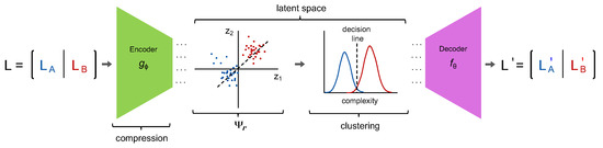
Figure 1.
Compression by a lossless encoder removes redundancy. The observations in L are then represented in the latent space defined by z and clustered according to their normalized compression distance [13]: a tractable approximation of the algorithmic complexity (image inspiration from [6]).
Returning to our hypothetical library , we can see how applying as an online algorithm could be used to refine L from a Library of Babel into a tractable library of primordial elements. In this way, where is the median (n.b., the mean can also be used but is less interpretable as medians correspond directly to entries in L) of the i-th cluster such that for and . It is important to make the distinction between the learned basis and . A good analogy is to think of as an alphabet, and K as a phrase book. To get an idea of the relative sizes of n, m, and r, the Oxford English Dictionary comprises words, while a typical English phrase book uses no more than words. Finally, there are letters in the English alphabet. In other words, K is a “Pareto optimal” starting point for communication.
Suppose, as depicted in Figure 1, we have two classes of objects, A and B. We can define their differences as the complexity of the shortest program that transforms A into B. This is known as the algorithmic complexity and is effectively a theoretical measure of distance between objects [14]. If we want to use prior observations to approximate unseen phenomena , then
(assuming target error is reached) where x is a coefficient vector of weights, and is the algorithmic (Kolmogorov) complexity between the observation and known morphemes. The number of morphemes needed to describe new object scales proportionally with the rarity (relative to the Kanji) of the object. Toward this end, a “good” Kanji should be large enough to not require too many morphemes such that description becomes impractical (n.b., a radix is an example of numeric Kanji. Binary is comprises 2 “morphemes” (i.e., 0,1); if we want to represent the number 134 in binary, we need to concatenate 8 characters (i.e., 10000110)—alternatively, in the decimal system, there are 10 morphemes such that we can represent the same information with 3 characters) and not too many as to be intractable (most native Japanese speakers are familiar with a couple thousand). While the original Kanji emerged naturally over thousands of years and captures complex and poetic themes that transcend quantitative analysis, modern machine learning methods contain all the necessary tools to “learn” a living Kanji via an online version of the process , given sufficient exposure to training data and assuming that all data types can be accepted by the autoencoder.
While a universal living Kanji for all past, present, and future knowledge will likely remain a dream of theorists and science fiction authors, it does not mean that learned reference libraries are infeasible for many domain-specific tasks. Fundamentally, the efficacy and tractability of learning a representative K is determined by the relative rarity of the observation. Consequently, if the amount of “surprising” data increases, then so must our access to unseen observations via the emergence of new basis modes embodying this newfound “surprise”. Toward this end, features expressed as combinations of novel basis modes, mined from the set of knowns, can be used to design optimized metrological equipment for future unknowns. This positive feedback loop will accelerate discovery by enabling the description of new observations. While up to this point, the discussion has been highly theoretical, in the following sections, we will review specific methods in machine learning and information theory with real-world applications. Additionally, we will show how these methods can be applied via concrete examples with different data types before concluding with an outlook toward a “fourth paradigm” for metrology in the era of big data.
2. An Information Theoretic Approach to Measurement
As discussed, the principle of factor sparsity states that the majority of a systems information is describable by a minority of the available content [15]. This creates an opportunity to exploit statistical regularities and construct inference models from far fewer observations. In the context of spectrometry, observed spectra are the result of the “vital few” interacting with many reflective and absorbing materials [16,17], making observed spectra naturally sparse (i.e., comprised of a few dominant signals). Signals that can be sparsely represented are also highly compressible [18], meaning that the information contained within the signal can be encoded by a much smaller number of non-zero coefficients in a representative transform basis. The observation that many natural phenomena are themselves sparse, is consistent with the atomic hypothesis and appears to be an axiom of our universe [19]. For metrology, the implication of this axiom is that if all natural signals can be reduced to an intrinsic dimension, then measurement devices (i.e., quantizers) should be defined relative to this latent space rather than an arbitrary rate.
When a signal is measured, it is quantized into discrete bits of information which can then be transmitted in an appropriate format. The sampling rate refers to the number of bits collected over some unit interval. Resolution, on the other hand, is the smallest detectable change typically defined over an interval [20]. A lossless quantizer will be able to resolve changes greater than or equal to without loss of information. As described by the Shannon–Nyquist sampling theorem [21], this specifies the sampling rate as being twice the minimum bandwidth of the signal (assuming the signal is bandlimited). The assumption that all signals are bandlimited is one of convenience, yet natural signals are inherently non-bandlimited. Consequently, every measured signal (adhering to Shannon–Nyquist theorem or not) is an approximation of the “true” signal, which we can only assume exists as a platonic form.
Another way to think about quantification is in terms of the intrinsic dimension, z, as illustrated in Figure 1. The intrinsic dimension is the number of features, or degrees of freedom, needed to uniquely describe all of the information comprised within the signal [22]. Recent advances in sparse representation and linear programming were able to demonstrate “sub-Nyquist” sampling by exploiting regularities in the intrinsic dimension via compressed sensing [23,24]. While compressed sensing is not, strictly speaking, inconsistent or a violation of the Shannon–Nyquist theorem, it is a viable approach to optimized sensing when signals are sparse relative to a generic transform basis. In practice, compressed sensing has transformed sensing across disciplines and established itself as the new baseline approach for many applications [25,26].
2.1. Intrinsic to What?
As we saw in Figure 1, the intrinsic dimension of an observation is defined by the latent space z such that the error between the input and output is minimized and below a predetermined error threshold. In the most general case, the latent space can be learned using deep autoencoder networks as a non-linear mapping. In most applications, a simple linear map defined by the singular value decomposition (SVD) is sufficient. Toward this end, for a given finite dataset of Ys, one can derive a set of eigen Ys by computing the principal components of the observation matrix Y. Functionally, these eigenvectors define a coordinate system aligned with the variance associated to Y. Alternatively, another way to approach the intrinsic dimension flirts with the sorites paradox wherein given a finite (quantized) signal, if one were to iteratively remove points along the distribution, at some iteration, for some set of selected and removed points, the signal becomes unrecoverable. If the points are equally distributed, we know when the breaking point occurs (i.e., according to Shannon–Nyquist), but this is less clear when deletion is neither random nor uniform.
In either case, the basis defines the low-rank approximation (an exact low-rank structure is rare). Here, comprises r modes “learned” from the singular values, .
We say is a “data-driven” or tailored basis [7] because it is derived from the original data matrix Y opposed to an “off-the-shelf”, universal, basis such as Fourier (n.b., we will distinguish data-driven bases from universal ones, with the subscript “r” indicating rank). The distinction between data-driven and universal bases is an important one that is closely related to interpretability. Universal bases are, by definition, generic and, therefore, removed from the structures and properties comprised within the signal. Each mode in a generic basis is “free” in the sense that graphemes are “free” from meaning as defined under the analogical concept interpretation [27]. Despite not (necessarily) being physically interpretable, data-driven basis modes are linked to specific structures and properties, thereby trading versatility for descriptivity and moving to a higher level of abstraction along the Pareto frontier (i.e., from grapheme to morpheme).
In order to illustrate the differences between data-driven and universal bases, let us take the example of finding the optimal sensor locations for encoding an observed high-dimensional signal. We suppose that the measurement process is modeled by a matrix P: , where . For a simple (1D) signal such as a normalized spectral power distribution, , the measured output is given by
The goal is then to use a universal or data-driven basis to reconstruct the measurement.
Unsurprisingly, determining the “best” P also depends on the type of basis used. For a signal measured at p points, reconstruction error is minimal when the sample locations correspond to the first non-zero p entries of P derived from a data-driven basis via QR factorization with column pivoting [7].
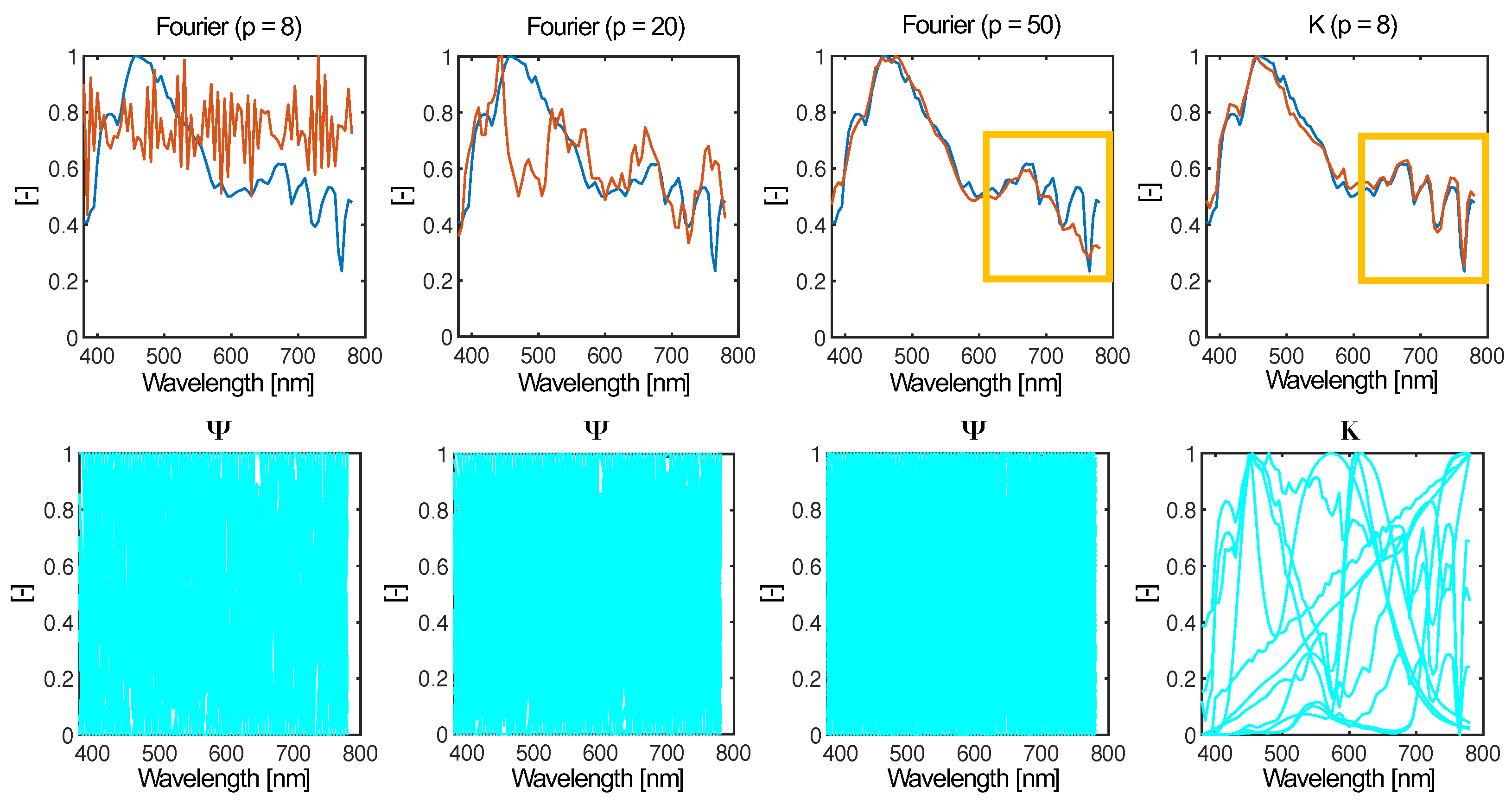
In the case when , QR factorization is much faster than conventional approaches to model order reduction (MOR) running on [7], compared to convex optimization methods [28] requiring per iteration. Toward this end, QR factorization is an attractive approach to optimal subset selection when the learned basis effectively captures features unique to the observed signals. The efficacy of a basis to span feature space does not necessarily increase with the size of the original data matrix (as is sometimes implied) but instead scales with the homogeneity of the set. As Y becomes more heterogeneous, the learned basis will become increasingly similar to a universal basis. In Figure 2, we can see this in action when we derive the basis for sets of normalized spectral power distributions. In this example, we derive via symmetric non-negative matrix factorization [29], which is an alternative MOR that has practical advantages for spectral sensing (discussed in the following section). Suffice to say, the basis modes are constrained to be non-negative, making them conceptually easier to interpret. In the four example sets we show, the number of modes is kept at . For each set of derived basis modes, we compute an index shown on the plot that evaluates the dissimilarity of the modes form fitted Gaussian radial basis functions. Higher values indicate that the basis modes are less Gaussian (and thus more “tailored” to the observations), which can also be seen upon visual inspection. While this observation is fairly trivial, it supports the idea that the structure of universal bases is emergent and primordial in that they represent forms that are shared amongst all observations. In the limit that a set equally expresses all possible features, the common denominator in any low-rank decomposition are universal basis modes.
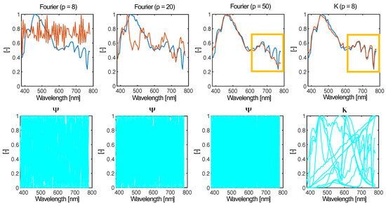
Figure 2.
The advantage of using a data-driven basis to solve the tailored sensing problem over classical compressed sensing illustrated in the reconstruction of a spectral power distribution sampled at different rates. Although the tailored library K contains fewer modes, enough shared features enable high-performance reconstruction, compared with generic Fourier modes (especially as seen in recovering the structure in the highlighted box).
The example in Figure 2 illustrates the core trade-off between data-driven tailored and universal bases, yet it should also be noted that the number of modes is fixed, and the efficacy of the derived bases to reconstruct their corresponding set of observations will not be the same. As the structure of the modes becomes more “normal”, the number of modes needed to retain reconstruction fidelity increases. This is reflected in the compressed sensing (CS) theorem [24,30] wherein given the reformalization of Equation (4), if we want to use a generic basis to recover a measured signal, then
can be solved via
In accordance with the CS theorem, reconstruction from p randomly sampled points is possible with high probability when , where n is the number of generic basis modes and K is the number of non-zero entries in x [31]. While there are a few subtleties we will not discuss (and which are better explained in [26]), the ingenuity of CS is that it allows for sub-Nyquist sampling without information loss by taking advantage of the compressibility of natural signals in a universal transform basis. In other words, the CS theorem demonstrates that for non-random signals, the intrinsic dimension of a single can be much smaller than previously understood under the classical interpretation of the Shannon–Nyquist theorem. In practice, this translates to sampling rates that can be roughly 10% of the classical Nyquist rate [6]. The key advantage of using generic bases is that no a priori knowledge of the structures or properties of the unknown signal is required. Therefore, representing a signal either in terms of the Nyquist rate or in terms of its sparse representation in a generic transfer basis are functionally identical.
From the perspective of information theory, CS presents a novel way of thinking about the intrinsic dimension of observables. It is an evolution of the Shannon–Nyquist theorem and a mathematical embodiment of Occam’s razor [32]. Within the context of the measurement of natural signals, such as light, CS provides the analytical framework needed to define the ground truth signal length over a specified range based solely on the amount of information comprised in the signal relative to the basis modes. In other words, as a general theory, CS can be used to set standards and norms on the minimal acceptable resolution and error () for measuring classes of natural signals. The problem with compressed sensing is two-fold; first, the advantage in sampling may not always be that competitive, especially when K is large. Second, because CS requires a universal basis and random sensor placement, there is no possibility of taking advantage of optimized sensor locations or informing the sampling protocol of devices via QR factorization.
2.2. Importance of Sparse Representation
Universality is typically a favorable property of bases for sparse representation, but in many real-world applications, total generality often results in overfit models. Nowhere is this more apparent than in the encoding of natural signals, which are well known to express statistical regularities [1]. Critically, universality ignores the truism that growth is the result of naturally occurring multiplicative processes [33], which are reflected in the regularities characterized by the distributions of Pareto and Zipf [34]. Toward this end, finding the “right” basis means balancing complexity and interpretability via a Pareto-efficient multi-objective optimization framework.
While CS sets strict theoretical limits on signal compressibility and, consequently, defines its intrinsic dimension, theorists realized that eschewing the statistical guarantees [35], by using data-driven bases and overcomplete dictionaries, can lead to dramatic increases in performance in practice [7]. Above all else, Equation (6) is tractable if, and only if, x is sparse and the properties placed on for CS are to ensure that sparsity is guaranteed without a priori knowledge of the underlying system. Since the seminal publication of CS in 2006, access to information has dramatically evolved, allowing researchers to mine extensive online libraries to build customized sparse representation dictionaries and data-driven bases via state-of-the-art machine learning methods. One method that is particularly well suited for CS is sparse dictionary learning (SDL), whose origins predate CS [36].
Like a basis, a dictionary is composed of basic elements. These basic elements are referred to in the literature as “atoms” in order to differentiate them from basis modes which form a linearly independent spanning set. This is the same distinction made previously between an alphabet of graphemes and a Kanji of morphemes. Practically, the SDL optimization problem is similar to Equation (7), wherein a dictionary K is learned for a given set of observations Y such that
and represents the error tolerance. The dictionary learning process can also be made into an online algorithm which has a number of advantages and is conceptually consistent with the idea presented in Section 1.2 that a dictionary or “Kanji” should evolve as new information is acquired. Additionally, online versions of conventional algorithms are becoming more common as streaming becomes an increasingly viable source of raw data [37]. The online dictionary learning (ODL) algorithm relies on the same optimization as above, such that the following holds:
- While ;
- Draw a new sample, , and initialize K and ;
- Find a sparse coding: ;
- Update dictionary: ;
- Update number of iterations: .
is a convex set of matrices constraining K, and is the i-th atom in the learned dictionary [38]. In this example, the initial dictionary is set to a random subset of our observational matrix Y. During each iteration, the optimization process adjusts the structure of these vectors slightly to find a better sparse representation. Consequently, after T iterations, the columns of K no longer resemble true observations, making them structurally more similar to cluster means. Toward this end, instead of finding the best subset of representative signals within a training set, SDL finds the most complete representation of each class of possible signals and balances information fidelity and interpretability much better than PCA.
The advantage of SDL as an online algorithm is that as datasets continue to grow, there is a high possibility that the elements in Y are naturally sparse, thereby requiring less deformation of the signals in the ansatz dictionary K. As we approach the limit where all possible signals are contained in Y, the computational burden is to find the fewest number d of representative spectra that contribute the most to a given observation (i.e., the vital few). By discarding structurally similar signals, a learned dictionary K offers real-world computational advantages. For this reason, big data can directly inform the best sparse representation for data-driven compressed sensing applications. While “big data” is often criticized as a wasteland of “digital garbage” [39], when used correctly, applications such as compressed sensing an SDL provide a framework to maximize the efficacy of large datasets.
3. Data-Driven Measurement
When the sparse representation basis is derived from prior observations, we refer to the reconstruction process as being data driven. In this section, we explore the data-driven cousins to the compressed sensing problem and investigate their potential impact on measurement. Let us start with a simple thought experiment: measuring the diameter of a coin. There are two approaches that one could take: measure the coin directly with a certified and calibrated device (e.g., a caliper), or identify the coin based on some features and look up its diameter, based on the observation that this coin belongs to a specific class of coins whose diameters are well known. The latter is a form of inference [40] and may be more efficient in practice, especially when the relevant domain knowledge is available. Suppose we expand the task to involve many coins; it will take much longer to measure each individually rather than using visual inspection to count and sort them before reporting the sizes for each class using a standard reference. Not only does this method require less physical hardware (no caliper needed), but the recorded data will comprise fewer bits, as class is a categorical and not continuous variable. Of course, this inference method only works when sufficient knowledge exists (i.e., after many coins have been measured) and therefore represents a data-driven approach. This simple example highlights an important observation: in the limit in which we have perfect information about a system, the effective intrinsic dimension of an observation is the minimum amount of information needed to differentiate it from all other known observations within that system [41]. Returning to the coin example, given that we know there is a finite number of possible coins, we only need to compile a set of feature arrays that uniquely define a coin within this finite set. Exchanging coins for any other data, we can imagine how increasing observational records can re-contextualize measurement as a classification problem.
The caveat for any data-driven method is that a sufficient number of measurements have to be made beforehand, either at or above the Nyquist rate (even if this is done through compressed sensing) in order to infer the underlying structures and properties of observations. To make an inference approach viable, a mathematical formalism is needed, and recent advances in signal processing are moving in this direction already. Tailored sensing can be thought of as an extension of compressed sensing to a data-driven basis [7]. To see how tailored sensing differs from compressive sensing, we can imagine three different scenarios: (1) we have no prior information (i.e., the cardinality of the set of prior information, ), (2) we have access to a prior observation () that is similar to what we intend to measure, and (3) we have multiple prior observations () that we can reference before we make a new observation. In the first case, we can sample at the compressed sensing rate , where K is the sparsity of the coefficient vector [31] and must use a generic basis for the reconstruction. In the second case, we still have to use a generic basis (a single signal is not sufficient to derive a tailored basis), but we can use the signal as a prior such that we can initiate the reconstruction process by telling the algorithm to start with solutions close to this previous observation [42]. Lastly, if we have access to a sufficient number of prior measurements (), we can use these measurements to derive a tailored basis by decomposing the matrix of prior observations into basic component elements (i.e., basis vectors). Under each of these three cases, the intrinsic dimension of the signal changes as a function of available domain knowledge. In other words, what defines the signal changes based on how much information is needed to differentiate it from all other signals. Therefore, in the limit that we have measured all possible signals, the intrinsic dimension of the signal would be the smallest lossless embedding.
3.1. Compressed Sensing with Prior Information
Fundamentally, the success of data-driven methods is predicated on the observation that the physical world is not random. Regularities, referred to in the literature as domain knowledge, and prior information, or simply priors, enable opportunities to more efficiently encode information. Priors are specifically interesting when collecting time-series data since samples taken at time () are not likely to differ significantly from a sample taken at t. Furthermore, the amount of information required to determine if the scene is changing is less than the information needed to capture the scene itself [43]. Many real-world applications are made simpler with prior information (e.g., video analysis). The compressed sensing problem with prior information (CSwP) can be written as
where is a generic basis matrix, x is a sparse coefficient vector, y is the measured output, w is a similar signal or prior, and is a positive coefficient balancing sparsity and prior information. This echoes the compressed sensing problem closely with only the addition of the prior information term. While there have been several methods proposed with similar approaches to the CSwP algorithm, it has been shown that the solution is optimized for and translates to 71% reduction in the required rate to recover the unknown information, compared to classical compressed sensing in specific compression tasks [42]. The more similar the prior is to the unknown signal, the smaller the amount of information required to capture its properties. In cases where observations distort within a predictable range, CSwP may provide significant advantages in encoder design and compression.
3.2. Tailored Sensing
Tailored sensing extends compressed sensing to further exploit statistical regularities in vast collections of previous observations [7]. The easiest way to derive a tailored basis is to apply PCA. As discussed, caution is advised, as the coordinate space formed by the PCA basis is abstract in the sense that it represents the uniquely identifying features without referencing specific physical properties of the signals themselves. While other matrix decomposition methods may be better suited depending on context (c.f., non-negative matrix factorization), PCA has routinely performed well for a diversity of applications [44]. Regardless, any orthogonal basis or overcomplete dictionary derived from the data will outperform generic methods if the data under investigation are similar to those used to derive the basis.
Unlike generic bases, the information encoded in the learned basis can also be used to determine sensor locations for optimized signal encoding. Returning to the coin analogy, we can look at historical records of coins to find the features that maximally discriminate them and define a classifier that looks for those specific traits. In practice, this means using the tailored basis to derive sensor locations that are optimally placed to capture the intrinsic properties of the signal. Recall that uniform sampling is penalized under the Shannon–Nyquist theorem at twice the effective bandwidth that compressed sensing requires. Tailored sensing only requires that the number of sample points is greater than or equal to the intrinsic rank of the data, which can be determined via Equation (2). Since the dominant columns of represent the majority of the information comprised in Y, we can use to infer the optimal sensor locations given that we will use as the basis for reconstruction.
The combination of tailored bases and QR factorization offers a robust framework for establishing data-driven metrological standards and norms. The derivation of P from is a direct and computationally light methodology that can inform directly the design properties of an encoder, thereby circumventing guesswork and assumptions based on uniform distribution or brute-force optimization. What P represents is as close as we can get to a standard observer for a specific class of signals. In the limit that number of prior observations goes to the infinite, P will become “generic” in the sense that it is optimized for all conceivable observations of its approved class (i.e., visible spectral power distributions).
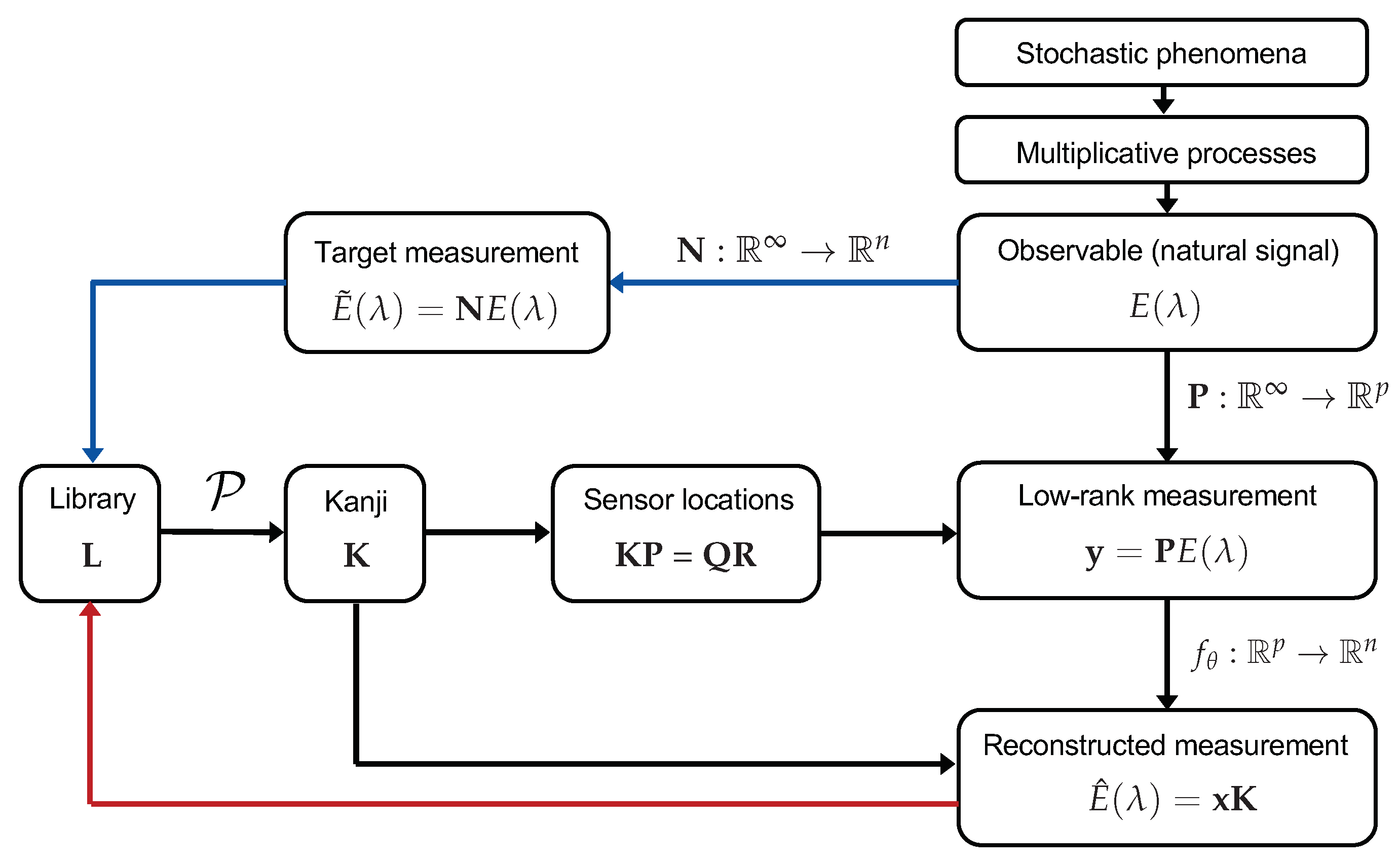
4. A Framework toward “Fourth-Paradigm” Metrology
What makes one observation different from another is highly non-trivial yet essential for constructing a system of measurement. Metrology has always relied on characterizing the unknown by the known, even if the choice of the known reference is one of convenience rather than rigor. Access to big data presents an opportunity to be rigorous with our choice of reference standard by applying dimension reduction algorithms to our increasingly vast datasets. From an information theoretic perspective, dissimilarity can be measured as the complexity, and by extension, information entropy, of the function that maps one observation to another [45]. Representing data collected from many natural systems with well-known statistical regularities in a data-driven basis is an increasingly viable approach with the opportunity to make significant improvements in the size and compressibility of measurements. In Figure 3, we sketch out how the concepts reviewed herein could be integrated into a singular data-driven framework.
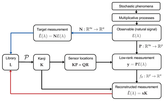
Figure 3.
An integrated framework for synthesizing new information into a tractable dictionary K and optimal encoder structure P. As data are collected, they are fed back into the overcomplete library. Process is expanded in Figure 1.
The framework outlined in Figure 3 optimizes both the dictionary (Kanji) K and the information encoder P. As L accumulates information, P will stabilize. In a way, P represents the ultimate standard observer, which is importantly capable of evolving with new information rather than being limited to a specific context or standard. While generic and universal bases have a role sparse representation, we should not ignore the potential of data-driven methods, especially considering how their relevance will continue to evolve, depending on the efficacy of MOR and other machine-learning methods.
5. Conclusions
Accelerating access to datasets across domains has led to a greater understanding of the patterns and regularities that comprise observable phenomena. If we think of all natural systems as unique configurations of low-dimensional dynamics, we can better characterize the structures and properties of highly complex systems. While measurement has traditionally been seen as objective, it is important to understand the limitations of a one-size-fits-all approach to standards and practices in metrology. In this review, we contextualized metrology through the lens of information theory by presenting methods to deconstruct heterogeneous signal populations into increasingly homogeneous basic elements. Specifically, we reviewed two approaches: compressed sensing and data-driven tailored sensing. While both are methods of sparse signal recovery, the former is axiomatically freer, while the latter is based on the existence of domain knowledge. Herein we have sketched out a proposed framework that connects ideas in MOR and sparse representation with the hope that metrology, in the context of “fourth-paradigm” ideology, may continue to evolve.
Author Contributions
Conceptualization, F.W.; investigation, F.W.; resources, M.A.; writing—original draft preparation, F.W.; writing—review and editing, F.W. and M.A.; visualization, F.W.; supervision, M.A.; project administration, M.A.; funding acquisition, M.A. All authors have read and agreed to the published version of the manuscript.
Funding
This research was funded by INNOSUISSE grant number 40598.1.
Institutional Review Board Statement
Not applicable.
Informed Consent Statement
Not applicable.
Data Availability Statement
Not applicable.
Acknowledgments
The authors thank Jeffrey Hubbard for his feedback on the manuscript.
Conflicts of Interest
The authors declare no conflict of interest.
References
- Kubin, G. What Is a Chaotic Signal? IEEE Workshop on Nonlinear Signal and Image Processing: Neos Marmaras, Greece, 1995. [Google Scholar]
- Vim, I. International vocabulary of basic and general terms in metrology (VIM). Int. Organ. 2004, 2004, 9–14. [Google Scholar]
- Wheeler, J. Gravity quantized? Sci. Am. 1992, 267, 20. [Google Scholar]
- Asimov, I. Foundation; Gnome Press: New York, NY, USA, 1951. [Google Scholar]
- Miller, R.A. Origins of the Japanese Language: Lectures in Japan during the Academic Year 1977–1978; University of Washington Press: Seattle, WA, USA, 1980. [Google Scholar]
- Brunton, S.L.; Kutz, J.N. Data-Driven Science and Engineering: Machine Learning, Dynamical Systems, and Control; Cambridge University Press: Cambridge, UK, 2019. [Google Scholar]
- Manohar, K.; Brunton, B.W.; Kutz, J.N.; Brunton, S.L. Data-driven sparse sensor placement for reconstruction: Demonstrating the benefits of exploiting known patterns. IEEE Control Syst. Mag. 2018, 38, 63–86. [Google Scholar]
- Borges, J.L. The library of Babel. Collected Fictions; Andrew Hurley Penguin: New York, NY, USA, 1998. [Google Scholar]
- Von Luxburg, U.; Williamson, R.C.; Guyon, I. Clustering: Science or art? In Proceedings of the ICML Workshop on Unsupervised and Transfer Learning, JMLR Workshop and Conference Proceedings, Bellevue, WA, USA, 28 June–2 July 2012; pp. 65–79. [Google Scholar]
- Mangan, N.M.; Kutz, J.N.; Brunton, S.L.; Proctor, J.L. Model selection for dynamical systems via sparse regression and information criteria. Proc. R. Soc. A Math. Phys. Eng. Sci. 2017, 473, 20170009. [Google Scholar] [CrossRef] [Green Version]
- Udrescu, S.M.; Tan, A.; Feng, J.; Neto, O.; Wu, T.; Tegmark, M. AI Feynman 2.0: Pareto-optimal symbolic regression exploiting graph modularity. arXiv 2020, arXiv:2006.10782. [Google Scholar]
- Pelleg, D.; Moore, A.W. X-means: Extending k-means with efficient estimation of the number of clusters. In Proceedings of the Icml, Stanford, CA, USA, 29 June–2 July 2000; Volume 1, pp. 727–734. [Google Scholar]
- Cilibrasi, R.; Vitányi, P.M. Clustering by compression. IEEE Trans. Inf. Theory 2005, 51, 1523–1545. [Google Scholar] [CrossRef] [Green Version]
- Bennett, C.H.; Gács, P.; Li, M.; Vitányi, P.M.; Zurek, W.H. Information distance. IEEE Trans. Inf. Theory 1998, 44, 1407–1423. [Google Scholar] [CrossRef]
- Murphy, K.P. Machine Learning: A Probabilistic Perspective; MIT Press: Cambridge, MA, USA, 2012. [Google Scholar]
- Chiao, C.C.; Cronin, T.W.; Osorio, D. Color signals in natural scenes: Characteristics of reflectance spectra and effects of natural illuminants. JOSA A 2000, 17, 218–224. [Google Scholar] [CrossRef] [Green Version]
- Webler, F.S.; Spitschan, M.; Foster, R.G.; Andersen, M.; Peirson, S.N. What is the ‘spectral diet’of humans? Curr. Opin. Behav. Sci. 2019, 30, 80–86. [Google Scholar] [CrossRef] [PubMed]
- Jacques, L. A short note on compressed sensing with partially known signal support. Signal Process. 2010, 90, 3308–3312. [Google Scholar] [CrossRef] [Green Version]
- Gribbin, J.; Gribbin, M. Richard Feynman: A Life in Science; Icon Books: Cambridge, UK, 2018. [Google Scholar]
- BIPM. Guide to the Expression of Uncertainty in Measurement; DIANE Publishing: Darby, PA, USA, 1993; Volume 94. [Google Scholar]
- Shannon, C.E. Communication in the presence of noise. Proc. IRE 1949, 37, 10–21. [Google Scholar] [CrossRef]
- Camastra, F.; Staiano, A. Intrinsic dimension estimation: Advances and open problems. Inf. Sci. 2016, 328, 26–41. [Google Scholar] [CrossRef]
- Candes, E.; Romberg, J. l1-magic: Recovery of Sparse Signals via Convex Programming. 2005. Available online: www.acm.caltech.edu/l1magic/downloads/l1magic.pdf (accessed on 26 December 2021).
- Candès, E.J. Compressive sampling. In Proceedings of the International Congress of Mathematicians, Madrid, Spain, 22–30 August 2006; Volume 3, pp. 1433–1452. [Google Scholar]
- Duarte, M.F.; Eldar, Y.C. Structured compressed sensing: From theory to applications. IEEE Trans. Signal Process. 2011, 59, 4053–4085. [Google Scholar] [CrossRef] [Green Version]
- Eldar, Y.C.; Kutyniok, G. Compressed Sensing: Theory and Applications; Cambridge University Press: Cambridge, UK, 2012. [Google Scholar]
- Kohrt, M. The term ‘grapheme’ in the history and theory of linguisticsv. In New Trends in Graphemics and Orthography; De Gruyter: Berlin, Boston, 1986; pp. 80–96. [Google Scholar]
- Joshi, S.; Boyd, S. Sensor selection via convex optimization. IEEE Trans. Signal Process. 2008, 57, 451–462. [Google Scholar] [CrossRef] [Green Version]
- Kuang, D.; Ding, C.; Park, H. Symmetric nonnegative matrix factorization for graph clustering. In Proceedings of the 2012 SIAM International Conference on Data Mining, SIAM, Anaheim, CA, USA, 26–28 April 2012; pp. 106–117. [Google Scholar]
- Donoho, D.L. Compressed sensing. IEEE Trans. Inf. Theory 2006, 52, 1289–1306. [Google Scholar] [CrossRef]
- Candès, E.J.; Romberg, J.; Tao, T. Robust uncertainty principles: Exact signal reconstruction from highly incomplete frequency information. IEEE Trans. Inf. Theory 2006, 52, 489–509. [Google Scholar] [CrossRef] [Green Version]
- Davenport, M.A.; Duarte, M.F.; Eldar, Y.C.; Kutyniok, G. Introduction to Compressed Sensing; Cambridge University Press: Cambridge, UK, 2012; Available online: https://assets.cambridge.org/97811070/05587/excerpt/9781107005587_excerpt.pdf (accessed on 19 December 2021).
- Otter, R. The multiplicative process. Ann. Math. Stat. 1949, 20, 206–224. [Google Scholar] [CrossRef]
- Pietronero, L.; Tosatti, E.; Tosatti, V.; Vespignani, A. Explaining the uneven distribution of numbers in nature: The laws of Benford and Zipf. Phys. A Stat. Mech. Its Appl. 2001, 293, 297–304. [Google Scholar] [CrossRef] [Green Version]
- Yin, P.; Lou, Y.; He, Q.; Xin, J. Minimization of 1–2 for compressed sensing. SIAM J. Sci. Comput. 2015, 37, A536–A563. [Google Scholar] [CrossRef] [Green Version]
- Kreutz-Delgado, K.; Murray, J.F.; Rao, B.D.; Engan, K.; Lee, T.W.; Sejnowski, T.J. Dictionary learning algorithms for sparse representation. Neural Comput. 2003, 15, 349–396. [Google Scholar] [CrossRef] [PubMed] [Green Version]
- Purohit, M.; Svitkina, Z.; Kumar, R. Improving online algorithms via ML predictions. In Proceedings of the 32nd International Conference on Neural Information Processing Systems, Montreal, QC, Canada, 3–8 December 2018; pp. 9684–9693. [Google Scholar]
- Mairal, J.; Bach, F.; Ponce, J.; Sapiro, G. Online dictionary learning for sparse coding. In Proceedings of the 26th Annual International Conference on Machine Learning, Montreal, QC, Canada, 14–18 June 2009; pp. 689–696. [Google Scholar]
- Che, D.; Safran, M.; Peng, Z. From big data to big data mining: Challenges, issues, and opportunities. In Proceedings of the International Conference on Database Systems for Advanced Applications, Wuhan, China, 22–25 April 2013; Springer: Berlin/Heidelberg, Germany, 2013; pp. 1–15. [Google Scholar]
- Estler, W.T. Measurement as inference: Fundamental ideas. Cirp Ann. 1999, 48, 611–631. [Google Scholar] [CrossRef]
- Kraskov, A.; Stögbauer, H.; Andrzejak, R.G.; Grassberger, P. Hierarchical clustering using mutual information. EPL Europhys. Lett. 2005, 70, 278. [Google Scholar] [CrossRef] [Green Version]
- Mota, J.F.; Deligiannis, N.; Rodrigues, M.R. Compressed sensing with prior information: Strategies, geometry, and bounds. IEEE Trans. Inf. Theory 2017, 63, 4472–4496. [Google Scholar] [CrossRef] [Green Version]
- Yin, J.; Liu, Z.; Jin, Z.; Yang, W. Kernel sparse representation based classification. Neurocomputing 2012, 77, 120–128. [Google Scholar] [CrossRef]
- Clark, E.; Brunton, S.L.; Kutz, J.N. Multi-fidelity sensor selection: Greedy algorithms to place cheap and expensive sensors with cost constraints. IEEE Sens. J. 2020, 21, 600–611. [Google Scholar] [CrossRef]
- Kolmogorov, A.N. On tables of random numbers. Sankhyā Indian J. Stat. Ser. A 1963, 25, 369–376. [Google Scholar] [CrossRef] [Green Version]

Publisher’s Note: MDPI stays neutral with regard to jurisdictional claims in published maps and institutional affiliations. |
© 2022 by the authors. Licensee MDPI, Basel, Switzerland. This article is an open access article distributed under the terms and conditions of the Creative Commons Attribution (CC BY) license (https://creativecommons.org/licenses/by/4.0/).