Article

Local Transformer Network on 3D Point Cloud Semantic Segmentation

1
Institute of Microelectronics, Chinese Academy of Sciences, Beijing 100029, China
2
University of Chinese Academy of Sciences, Beijing 100049, China
*
Author to whom correspondence should be addressed.
Information 2022, 13(4), 198; https://doi.org/10.3390/info13040198
Submission received: 19 February 2022 / Revised: 25 March 2022 / Accepted: 2 April 2022 / Published: 14 April 2022
(This article belongs to the Topic Big Data and Artificial Intelligence)

Abstract

:
Semantic segmentation is an important component in understanding the 3D point cloud scene. Whether we can effectively obtain local and global contextual information from points is of great significance in improving the performance of 3D point cloud semantic segmentation. In this paper, we propose a self-attention feature extraction module: the local transformer structure. By stacking the encoder layer composed of this structure, we can extract local features while preserving global connectivity. The structure can automatically learn each point feature from its neighborhoods and is invariant to different point orders. We designed two unique key matrices, each of which focuses on the feature similarities and geometric structure relationships between the points to generate attention weight matrices. Additionally, the cross-skip selection of neighbors is used to obtain larger receptive fields for each point without increasing the number of calculations required, and can therefore better deal with the junction between multiple objects. When the new network was verified on the S3DIS, the mean intersection over union was 69.1%, and the segmentation accuracies on the complex outdoor scene datasets Semantic3D and SemanticKITTI were 94.3% and 87.8%, respectively, which demonstrate the effectiveness of the proposed methods.

1. Introduction

The semantic segmentation of 3D point clouds is one of the key problems in the perception of environments in the research on robotics [1] and automatic driving [2]. The use of local and global geometric attributes of a point to generate an effective feature description of the point, thereby improving the accuracy of semantic segmentation, has always been the focus and challenge in this field.
Convolutional neural networks (CNNs) have achieved great success in 2D imaging, with researchers considering how to use a mature CNN network to analyze 3D point clouds. However, unlike 2D images, point clouds are unordered and irregular, which make handling 3D point clouds using a convolutional neural network directly impossible. Some methods [3,4,5,6,7] project the 3D point clouds onto the 2D plane, generating a bird’s eye view (BEV) image, a range view (RV) image, and other intermediate regular representations, and then use them in a convolutional neural network. This kind of method depends on the choice of projection angle, which cannot make full use of accurate spatial and structural information and causes a loss of geometric information in the projection process. The method based on discretization converts the point clouds into a discretized representation, such as a voxel or lattice, and then processes it using a three-dimensional convolution network. However, it is sensitive to voxel size. When the voxel is large, it causes information loss and affects the segmentation accuracy. When the voxel is small, it leads to a sharp increase in the number of calculations required and affects the real-time performance. The point-based method extracts features directly from irregular point clouds without any preprocessing. It has gradually become the mainstream method used in point cloud semantic segmentation. However, the point-based method also has some problems, such as the poor scalability of the point sampling method to the scale of the point cloud, and the inability to effectively learn local features.
With the successful application of a self-attention mechanism in the field of natural language processing (NLP), some studies have considered the applications of the transformer structure to the fields of image and point cloud processing, etc. The input of a transformer is usually a sequence, and position embedding information needs to be added. For point cloud data, each point has a unique coordinate value, which can be directly used as the position embedding information. Zhao et al. [8] proposed the point transformer and proved that a network structure based entirely on self-attention can effectively solve a point cloud task.
The transformer method has been broadly used for object-wise tasks, such as classification and partial segmentation. Inspired by these works, in this study, we use a transformer network for point-wise large-scale point cloud segmentation. We propose a novel multi-scale transformer network for both local and global feature extraction.
The network is based on an encoder–decoder structure. Each encoder layer consists of two parallel local transformers. In the front of the encoder layers, local features can be obtained because of the locality of the local transformer. After random down-sampling of the points, the receptive field of each point becomes larger and every point contains high-level features. Therefore, at the later encoder layers of the encoder, the global features can be easily obtained by the local transformer structure, making full use of the transformer having no inductive bias property.
In contrast to a previous transformer structure with one attention weight matrix, which can find the similarities between point features, we propose two different key matrices to obtain two attention weight matrices in the local transformer structure, which can not only focus on the feature similarity between points but also focus on the local geometric structure relationship. The results of the visualization show that better segmentation results can be obtained between objects with very similar geometries. We also propose two fusion strategies to make full use of the distribution diversity of these two attention weight matrices.
In order to improve the segmentation performance at the semantic edges of multiple objects, we propose a novel neighbor selection method called cross-skip selection, which is very suitable for the parallel encoder layer, and can expand the receptive field of each point without increasing the number of calculations required, and capture more abundant geometric and semantic information.
We then verified our method on open datasets S3DIS and Semantics3D. The best mean class-wise intersection over union (mIoU) on the S3DIS dataset was 69.1% and on the Semantic3D dataset was 75.7%, which are better than those of most benchmark methods.
Our contributions can be summarized as follows:
  • We propose a novel multi-scale transformer network to learn local context information and global features, which makes applying the transformer on more sophisticated tasks from the large-scale point cloud datasets possible.
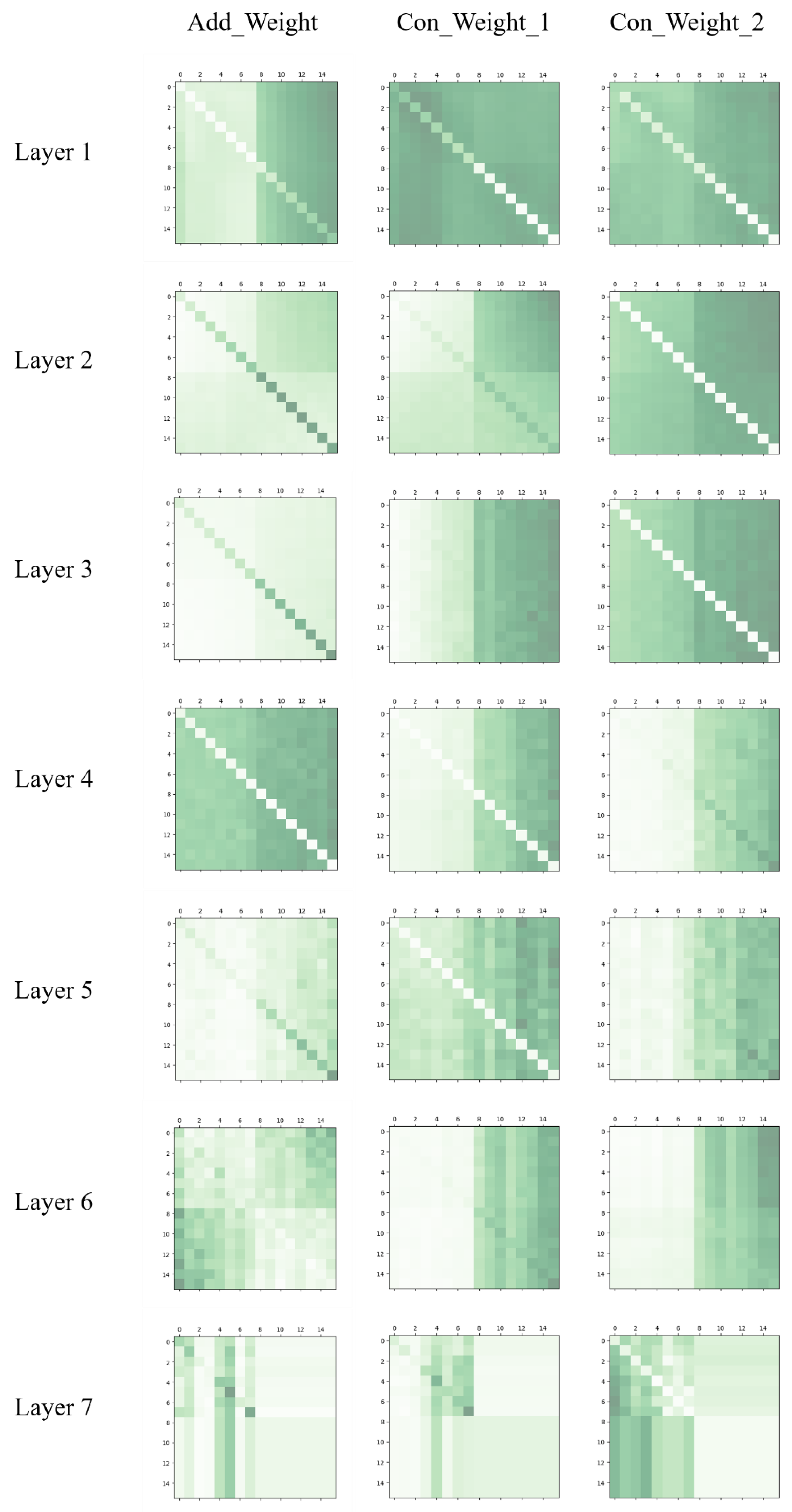
  • In order to obtain the feature similarity and local geometry relationship between points, we propose two different key matrices to obtain two attention weight matrices in the local transformer structure, and propose two different fusion strategies to fuse them.
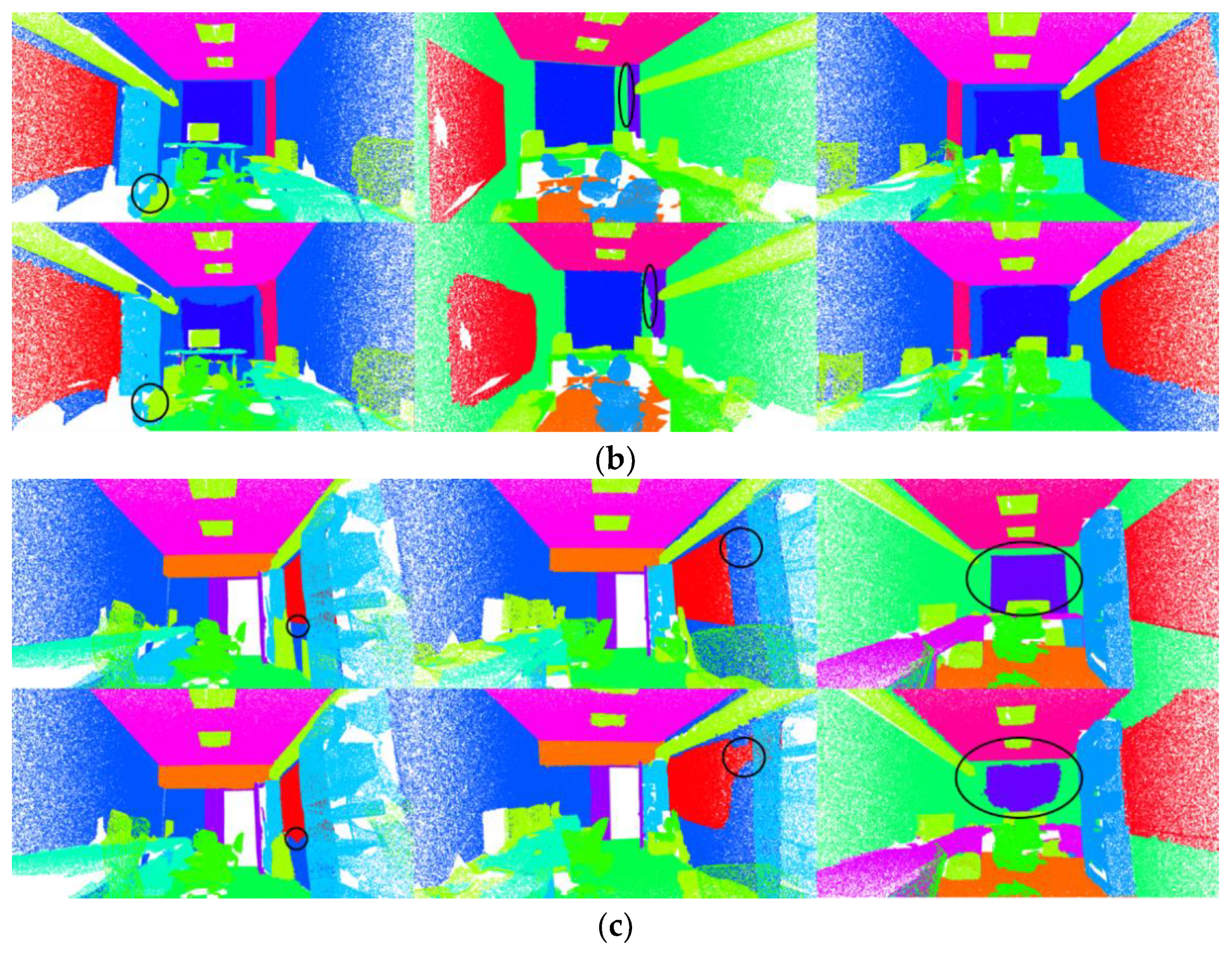
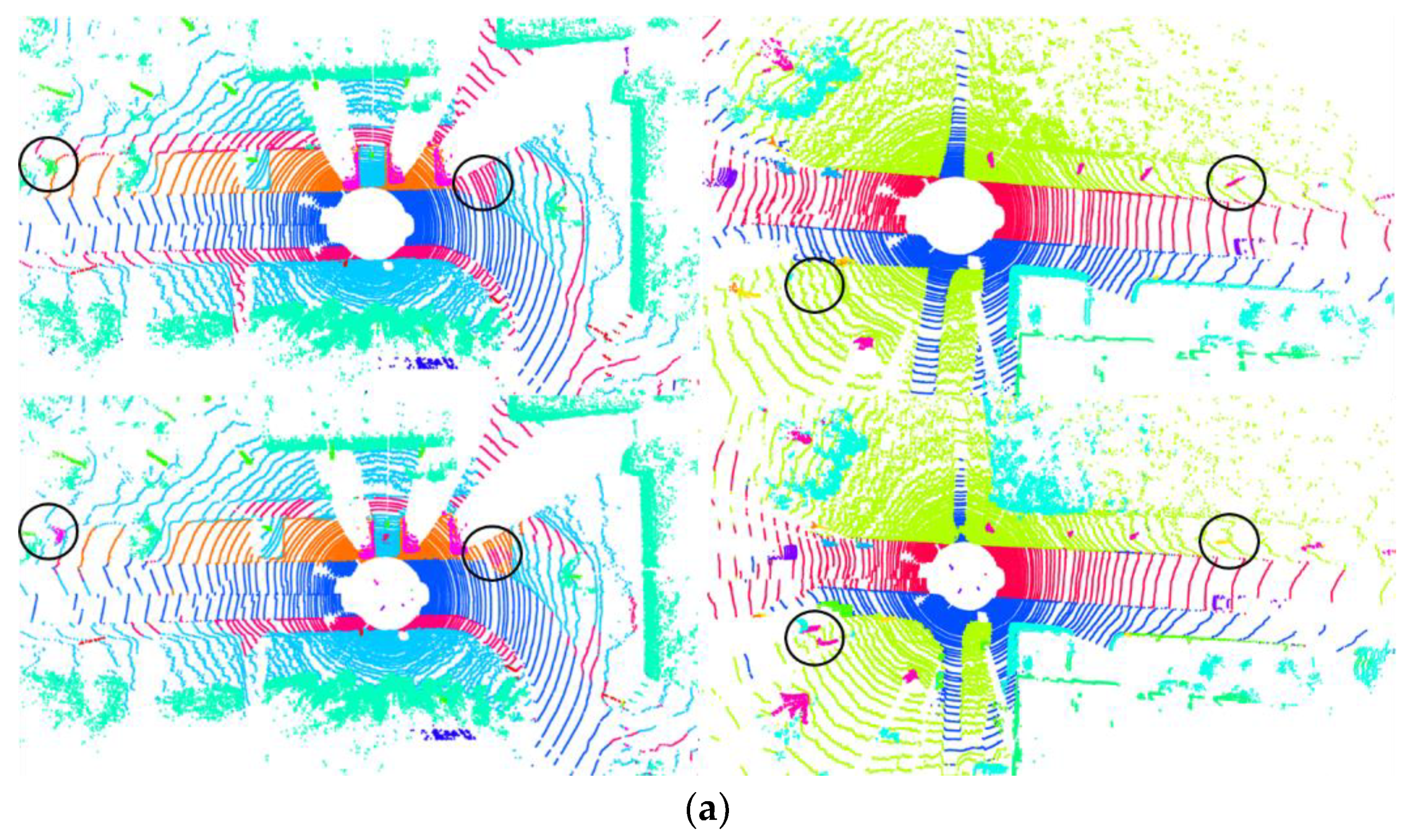
  • We also propose a novel neighbor selection method called cross-skip selection to obtain more accurate results on the junction of multiple objects.
The rest of the paper is organized as follows. Section 2 presents related work on 3D point cloud semantic segmentation. Section 3 presents our proposed approach, including the network architecture (Section 3.1), neighbor embedding module (Section 3.2), feature extraction module based on a transformer (Section 3.3), local transformer structure (Section 3.4), parallel encoder layer with cross-skip selection (Section 3.5), and decoder layer (Section 3.6). Section 4 presents our experiments and analysis. Section 5 concludes our work and presents some future work.

2. Related Work

According to the different forms of input point clouds, the semantic segmentation methods of a point cloud can be divided into the projection-based method, the discretization-based method, the point-based method, etc.
The projection-based method is used to project the 3D point cloud onto the 2D plane. Rangenet + + [9] first converted the point cloud into a range image, then used the full convolution network to deal with that, and then mapped the result of the semantic segmentation to the original point cloud. Squeezeseg [10] converted the point cloud to the front view through spherical projection, using the SqueezeNet network for semantic segmentation, and then used a conditional random field (CRF) to refine the results. Liong et al. [11] proposed a multi-view fusion network (AMVNet), which projected the point cloud onto the range view (RV) image and bird’s eye view (BEV) image, and combined the advantages of using two different views of RV and BEV.
VoxNet [12] is a typical discretization-based method. The network divided the point cloud into regular voxels and then extracted the features of these voxels through a 3D convolution operation. However, the point cloud is sparse, and the proportion of non-empty voxels is very small. It is very inefficient to use a dense convolution neural network on spatial sparse data. Graham et al. [13] improved this by proposing a new sparse convolution operation that can process spatial sparse data more effectively.
PointNet [14] was the pioneer work that directly consumed point clouds, and could obtain per-point features by concatenating features learned by the shared multilayer perceptron (MLP) and global features learned by max pooling function. However, PointNet cannot effectively obtain local features and ignores the local context information. The PointNet + + [15] network made some improvements. It paid attention to the relationship between the central point and its neighbors but ignored the relationship between each neighbor pair. Wu et al. [16] proposed a new convolution operation, which defined the convolution kernel as a nonlinear function composed of a weight function and a density function. Zhao et al. [17] proposed a network called PointWeb, which can specify the feature of each point based on the local region characteristics for better representing the region. KPConv [18] defined an explicit convolution kernel, which is composed of fixed or flexible core points. The different weights of influence for each neighbor point on the core point adaptively depends on the distance between them. Hu et al. [19] used MLP to learn the attention weight score of each point and then obtained the weighted local feature map. Finally, the maximum pooling function was used to calculate the central point feature on the weighted local feature map.
In addition, there are some other methods. For example, the dynamic graph convolutional neural network (DGCNN) [20] uses graph networks to capture the local geometric features of a point cloud and dynamically updates a graph to learn the different scale features. Wang et al. [21] proposed a graph attention convolution (GAC), in which the kernels can be dynamically carved into specific shapes to adapt to the structure of an object and generate more accurate representations of local features of points.
Recently, the transformer network has already achieved tremendous success in the language domain; thus, most researchers want to investigate whether it can be applied to computer vision tasks. It is very encouraging that some methods [22] showed that a pure transformer applied directly to sequences of image patches can perform very well on image classification tasks. After that work was conducted, research on transformers in computer vision became popular. The operator of the transformer network is invariant to permutation, making it particularly appropriate for point clouds, since a point cloud is permutation-invariant.
Some recent work considered how to effectively extract local and global features at the same time. LocalViT [23] aimed to combine the local performance of a convolutional neural network and the global connectivity of a transformer structure. However, using a transformer structure to learn the long-distance dependence between points requires very high memory and expensive computing costs, which make it difficult to deal with large-scale 3D point cloud data. In this paper, we propose a local transformer structure and a novel neighborhood sampling method for local feature extraction; it can not only effectively focus on local features, but also reduce the computational costs to adapt to the semantic segmentation tasks of large-scale outdoor datasets.

3. Proposed Approach

3.1. Network Architecture

The overall network structure adopts the typical encoder–decoder structure [24]. The encoder is composed of parallel encoder layers (Section 3.5), which consist of two local transformer structures (Section 3.4). The local transformer structure is composed of a neighbor embedding module (Section 3.2) and a feature extraction module based on a transformer (Section 3.3). As shown in Figure 1, after each parallel encoder layer, random down-sampling is used to reduce the number of points and then to stack parallel encoder layers. As the encoder layers are stacked, the semantic features of each point become more and more abstract and contain more contextual information. We set up a different number of encoder layers for different datasets. Then, the number of points is recovered through the decoder layers. In this paper, we use a distance-based weighted linear interpolation up-sampling operation (Section 3.5) to propagate the features from a sparse point cloud to a dense point cloud to predict point-wise labels. The whole network structure adopts a residual connection.

3.2. Neighbor Embedding Module

Point-wise local geometric properties, such as the normal vector (the normal vector of each point is the normal direction of the plane fitted by it and its neighbors), are very useful for discovering the similarity between points, since the normal vector of the surface of an object changes continuously. Before the data are input into the network, we compute the normal vector of S3DIS and combine it with their corresponding point coordinates as a rich feature representation. We use principal components analysis (PCA) to compute the normal of every point (as shown in Figure 2). For each point, we choose its M neighbors P : { p 1 , p 2 , p M } R M × 3 . We want to fit a plane using the M neighbors, and then, we can calculate the normal vector of the point. The normal vector is solved by minimizing an objective function as follows:
m i n c , n , | | n | | = 1 i = 1 M ( ( p i c ) T n ) 2 ,
c = 1 M i = 1 M p i ,
where c is a coordinate of the center of all neighbor points and n is the normal vector to be solved.
The input point cloud is represented as a coordinate matrix P : { p 1 , p 2 , p N } R N × 3 and its feature matrix F : { f 1 , f 2 , f N } R N × D . N and D are the number of points and the feature dimensions, respectively. The original input features of the points are concatenated by the normalized x-y-z coordinates, raw RGB, and surface normal information.
First, we encode the local region in the neighbor embedding module, as shown in Figure 3, similar to a reference point x i , and find its 2 K neighbors, encoding each neighbor point to obtain its position embedding G : { g i 1 , g i 2 , g i 2 k } R 2 K × D , as shown in Formula (3). g i k is the position embedding of the k -th neighbor.
g i k = ( p i p i k ) | | p i p i k | | .
where stands for the concatenation of ( p i p i k ) and | | p i p i k | | on the feature dimension, p i is the coordinate of the point x i , p i k is the coordinate of the k -th neighbor, and | | · | | is the l 1 norm.
Then, the local region feature matrix I i n : { I i 1 , I i 2 , I i 2 k } can be obtained by concatenating the positional embedding g i k and per-point original features f i k as follows:
I i k = M L P ( g i k ) M L P ( f i k ) .
where M L P ( · ) is a multilayer perceptron applied to the positional embedding g i k and features f i k .

3.3. Feature Extraction Module based on a Transformer

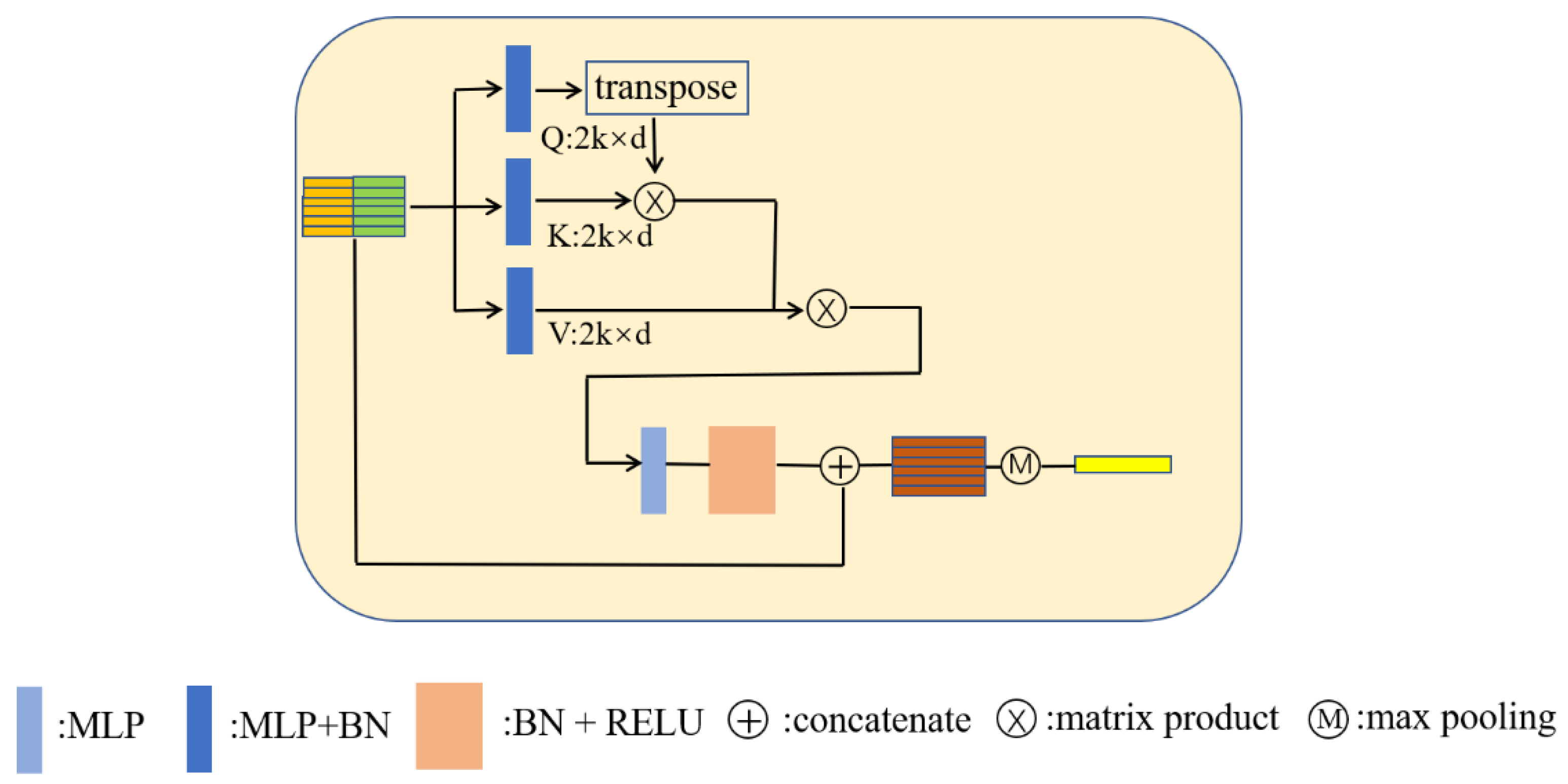
3.3.1. Naïve Transformer Structure

Using the neighbor embedding module, we can obtain the local region feature matrix: I i n R 2 k × d i n ( d i n is the dimension of the features). It is then input into a transformer structure to obtain the weighted features of the reference point. In the naïve transformer structure, Q , K , V are obtained based on I i n , as shown in Formula (5).
Q = B N ( M L P 1 ( I i n ) ) ,   K = B N ( M L P 2 ( I i n ) ) ,   V = B N ( M L P 3 ( I i n ) ) ,   Q , K , V R k × d
where B N ( M L P ( · ) ) stands for a batch normalization operation after a multilayer perceptron. The batch normalization normalizes the batch input on the feature dimension. It can make the distribution of input data in each layer of the network relatively stable and accelerates the learning speed of the model. d is the dimension of Q , K , V . We set the dimensions of Q , K , V to be equal.
The attention score is computed as the inner product between Q and K . The attention weight matrix can be written as follows:
W = ( w ˜ i j ) = Q · K T .
Additionally, a scale and a normalization operation, which is able to obtain measurements of the similarity between any two points in this local region, can be used:
w ¯ i j = w ˜ i j d ,
w i j = s o f t m a x ( w ¯ i j ) = exp ( w ¯ i j ) k exp ( w ¯ i , k ) .
Next, the normalized attention weight matrix is applied on the value matrix V to obtain a weighted local feature matrix, which can automatically assign more attention to the useful features. The weighted local feature matrix can be written as follows:
I w = W · V ,   I w ϵ R 2 k × d .
Then, we use batch normalization and non-linear activation on this weighted local feature matrix. After that, we concatenate the activated features matrix and the original input features matrix as follows:
I 1 = L B R ( I w ) I i n ,   I 1 R 2 k × 2 d i n .
where LBR is the normalization and non-linear activation operation and is the concatenation operation.
We use a symmetric operation such as max pooling to generate the reference point features, which can represent this local region. It is formally defined as follows:
I o u t = M L P ( m a x p o o l i n g ( I 1 ) ) ,   I o u t R 1 × d o u t .
Figure 4 provides an illustration of the naïve transformer structure. Through this transformer, the updated features of each reference point adaptively aggregate the features of its neighbor points.

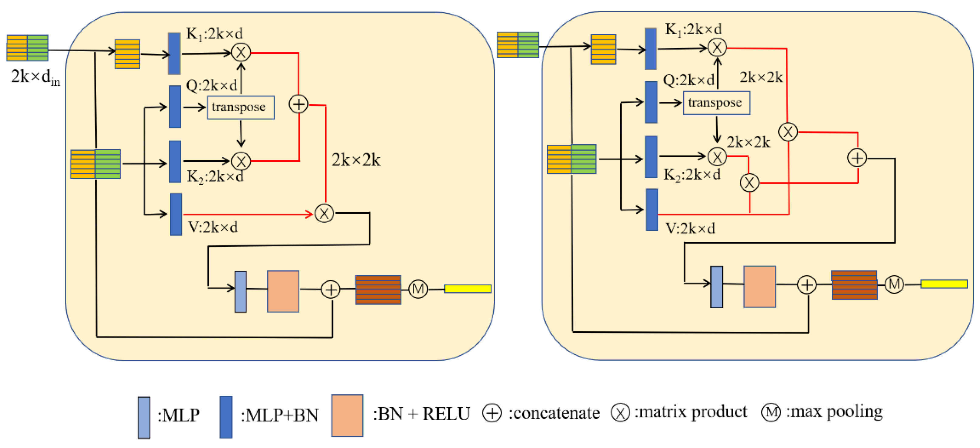
3.3.2. Improve Transformer Structure

We make some improvements to the naïve local transformer structure. Consider that, during the beginning of the network, where each point has not learned enough features yet to obtain the similarity between points, the geometric relationships between points become more significant than the features. Therefore, we propose two different key matrices for obtaining two attention weight matrices. The first key matrix is the same as the naïve local transformer structure, which is obtained by the input feature matrix I i n , as shown in Formula (12):
K 1 = B N ( M L P ( I i n ) ) , K 1 R 2 K × d .
The attention weight matrix can be written as Formula (13), which can obtain the feature similarity between points:
W 1 = ( w 1 ) i j = Q · K 1 T .
The query matrix Q can be obtained by Formula (5).
The second key matrix, which is obtained by the neighbor position embedding matrix G : { g i 1 , g i 2 , g i 4 k } R 2 K × D , takes the local geometry relationship into account. The second key matrix can be written as follows:
K 2 = B N ( M L P ( G i n ) ) , K 2 R 2 K × d .
The second attention weight matrix is as follows and can pay more attention to the local geometry relationship between points than W 1 :
W 2 = ( w 2 ) i j = Q · K 2 T .
When the two attention weight matrices are obtained, the most intuitive method for combining them is to add them, which can be shown as follows:
W a d d = W 1 + W 2 .
The next operations are the same as the naïve local transformer structure. Finally, we can obtain the weighted local feature matrix.
I w = W a d d · V , I w R 2 K × d .
where V is the key matrix, which can be obtained using Formula (5).
However, if we simply add the two attention weight matrices together, we cannot make full use of the distribution diversity of the two attention weight matrices. We propose another fusion method at the feature level. Specifically, we multiply the two scaled and normalized attention weight matrices with the value matrix, as shown in (18) and (19), respectively, and then concatenate the weighted local feature matrices, as shown in (20).
I w 1 = W 1 · V , I w 1 R 2 K × d ,
I w 2 = W 2 · V , I w 2 R 2 K × d ,
I w = I w 1 I w 2 , I w R 2 K × 2 d .
where V is the key matrix, which can be obtained using Formula (5).
By fusing at the feature level, we can obtain weighted feature matrices I w 1 and I w 2 with two different distributions, which can inherently capture the features and geometric relationships between points.
The updated point feature I o u t can finally be obtained using the operations in (10) and (11) on I w . The improved transformer structures are shown in Figure 5:
We also visualized the attention weight matrices, presented in Appendix A. From the results of the visualization, we can note that, at the first few layers, W a d d shows a locality (the value of the diagonal is significantly different from the others) and, at the last two layers, it shows a discretized distribution, which can be used to find points with key semantic information. When we fuse the attention weight matrices at the feature level, at every layer, W 1 and W 2 focus on the feature similarities and the geometry relationship between points, respectively. Therefore, they have different distributions.

3.4. Local Transformer Structure

The local transformer structure is composed of a neighbor embedding module and a transformer structure, which is shown in Figure 6.

3.5. Parallel Encoder Layer with Cross-Skip Selection
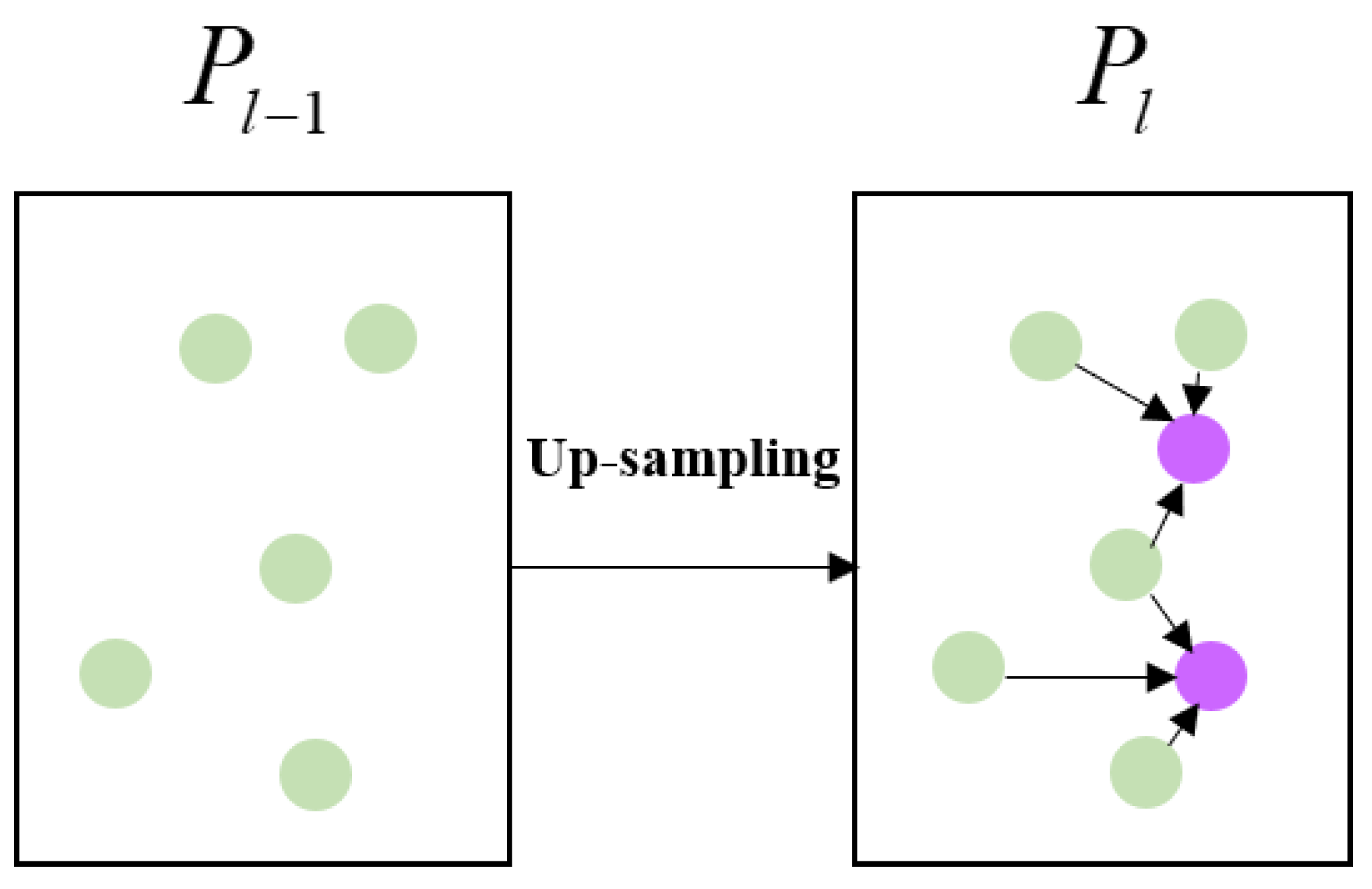
The distance and feature similarities between each point and its neighbors are not necessarily positively correlated, especially at the junction of multiple objects. Therefore, points with similar semantic structures may have greater Euclidean distances and vice versa. As shown in Figure 7, the distance between c 1 and c 1 is greater than that between c 1 and c 2 , while c 1 and c 1 belong to class 1 and c 2 belongs to class 2.
We propose a cross-skip selection method to obtain neighbors in the neighbor embedding module. The method is as follows: find the nearest 4 K neighbor points of each point and divide them into four groups k 1 , k 2 , k 3 , k 4 with the same number. Each group contains K points. Concatenate the point feature in k 1 and in k 3 , k 2 , and k 4 , and then encode the two original point feature matrices in the neighbor embedding module to obtain the local region feature matrices I i n 1 and I i n 2 .
In order to adapt to the cross-skip selection method, we propose a parallel encoder layer composed of two parallel local transformer structures, as shown in Figure 8. The two input matrices of the same dimension I i n 1 and I i n 2 are composed of different neighbor points selected based on cross-skip selection. This structure allows each point to obtain a larger receptive field without increasing the dimension of the input matrices I i n 1 and I i n 2 . Concatenate the two update feature vectors I o u t 1 and I o u t 2 to obtain the final output I o u t .
I o u t = I o u t 1 I o u t 2 .

3.6. Decoder Layer

To finally obtain each original point feature, we simply adopt a distance-based weighted linear interpolation up-sampling operation, shown in Figure 9. Let P l 1 and P l be the coordinate set of the ( l 1 ) -th layer and ( l )-th layer at the decoder block, respectively. To obtain the feature of point p i at P l , we search the nearest three neighbors ( t = 3 ) of p i in P l 1 . The coordinates of neighbors are p i t = { p i 1 , p i 2 , p i 3 } , and we obtain the influence of each neighbor point on p i based on the distance between the point p i and p i t = { p i 1 , p i 2 , p i 3 } , as follows:
M i j = ( m i j ) = M L P ( | | p i p i j | | ) .
where M i j is the influence weight and p i j is the coordinate of the j -th neighbor of the point p i .
Finally, the feature of p i is as follows:
f i = j = 1 3 m i j p i j .
where m i j is the weight of influence for each neighbor point obtained by Formula (22).

4. Experiments and Analysis

4.1. Datasets

S3DIS [25]: the Stanford 3D Large-Scale Indoor Spaces (S3DIS) dataset addresses semantic tasks with pixel-level semantic annotations developed by Stanford University. It consists of six areas, each of which contains 13 categories such as ceiling, floor, and wall. We evaluated our network using two methods: (1) six-fold cross-validation and (2) area 5 testing. Moreover, we used the mean class-wise intersection over union (mIoU), the mean of class-wise accuracy (mAcc), and the overall point-wise accuracy (OA) as evaluation metrics.
Semantic3D [26]: the Semantic3D dataset is composed of 30 non-overlapping outdoor point cloud scenes, of which 15 scenes are used for training and other scenes are used for online testing. The dataset contains eight categories. The scenes cover rural, urban, and suburban areas, and each scene covers sizes of 160 × 240 × 30 . In addition to 3D coordinates, the dataset provides RGB values and intensity values. We used the mean class-wise intersection over union (mIoU) and the overall point-wise accuracy (OA) as evaluation metrics.
SemanticKITTI [27]: the SemanticKITTI dataset is composed of 21 sequences and 43,552 densely annotated laser scanning frames. Among these, sequences 00–07 and 09–10 are used for training, sequence 08 is used for verification, and sequences 11–21 are used for online testing. The raw data contain the 3D coordinate information of the points. We used the mean class-wise intersection over union (mIoU) as an evaluation metric.

4.2. Implementation Details

When verifying the proposed model based on the S3DIS dataset, we first obtained the normal vector of each point as the original feature. We set the number of encoder layers as 7. After each layer extracts the characteristics of each point through the encoder layer, random down-sampling is used to reduce the number of points. The random down-sampling is more efficient than other down-sampling methods, which have a high calculation cost and high GPU memory requirements. We set the sampling ratio to [2, 2, 4, 4, 4, 4, 4] and the output dimension of each layer to [16, 64, 256, 256, 512, 512]. Through distance-based weighted interpolation linear up-sampling, three nearest neighbors are selected to restore the feature of the input points. Finally, three fully connected layers are stacked to obtain the output with a category number dimension. When verifying the model on the SemanticKITTI and Semantic3D datasets, because the number of points in each frame is very large, calculating the normal vector of each point consumes a very large amount of memory, so we only calculate the normal features in an indoor dataset.
In addition, we used a residual connection to retain more point feature information. In this paper, the Adam optimizer and weighted cross entropy loss based on inverse frequency were used for training. All experiments used Tensorflow as the platform and applied an NVIDIA Corporation gp102 (Titan XP) GPU.

4.3. Evaluation Metrics

For the S3DIS dataset, the mean class-wise intersection over union (mIoU), mean class Accuracy (mAcc), and Overall Accuracy (OA) of the total 13 classes were compared. For Semantic 3D, the mIoU and OA were used as the evaluation metrics. For SemanticKITTI, we used mIoU. The evaluation metrics can be defined as follows:
m I o U = 1 k + 1 i = 0 k p i i j = 0 k p i j + j = 0 k p j i p i i ,
O A = 1 N i = 0 k p i i ,
m A c c = 1 k + 1 i = 0 , j i k p i i p i j .
where k + 1 is the number of classes, i is the ground-truth label, j is the prediction label, p i j is the number of the samples that belong to i but are mistakenly predicted as j , p j i is the number of the samples that belong to j but are mistakenly predicted as i , p i i is the number of correctly predicted samples, and N is the total number of samples.

4.4. Experimental Results

We used area 5 of S3DIS for testing and the other areas for training. The results are shown in Table 1. Table 2 shows the results with six-fold cross-validation. Table 3 and Table 4 show the results on the Semantic3D and SemanticKITTI datasets, respectively. The results show that the proposed method is better than most benchmark models. The results of the visualization on S3DIS and SemanticKITTI are shown in Figure 10 and Figure 11.

4.5. Ablation Experiment

4.5.1. Naïve Local Transformer Structure and Improved Local Transformer Structure

Table 5 shows a comparison of the performances between the naïve local transformer structure and the improved local transformer structure on the S3DIS dataset. In the ablation experiment, we fused the two attention weight matrices by adding them. The experiment results proved the importance of adding the key matrix obtained by the position embedding matrix. Using the improved local transformer structure, OA improved by 0.8%, mAcc improved by 1.6%, and mIoU improved by 1.5%.
The results of the visualization are shown in Figure 12. According to these results (the part circled in the figure), it can be seen that between some objects in which the geometric structures are too similar and cause confusion (such as walls and windows, and walls and doors), the improved local transformer structure (adding the attention weight matrix to explore the geometric relationship) obtains better segmentation results than the naïve local transformer structure.

4.5.2. Cross-Skip Selection Method

Our experiments verified the effectiveness of the cross-skip selection of neighbors. The results are shown in Table 5. The OA will increase by 0.6%, mAcc will increase by 1.8%, and mIoU will increase by 1.6%. The results of the visualization are shown in Figure 13. At the junction between objects, the similarity between points is not necessarily positively correlated with the distance between them. Points belonging to different objects may interfere with each other and affect the segmentation performance. Using cross-skip selection of the neighbors can expand the receptive field of each point. The results of the visualization are shown in Figure 14. In the places marked in blue circles, using this method will obtain better segmentation results.

4.5.3. Normal Feature

Table 5 shows a comparison between the results when using and not using normal vector features on the S3DIS dataset. It can be found that, after using normal vector features, OA will be improved by 0.5%, mAcc will be improved by 3%, and mIoU will be improved by 2.5%. This is mainly due to the fact that the normal vectors of most points belonging to the same object are similar or continuously changing.

5. Conclusions

In this paper, we first proposed a muti-scale transformer network for semantic segmentation of a 3D point cloud. This network structure can effectively extract the local and global features of a 3D point cloud. Second, in the local transformer structure, two different attention weight matrices are obtained, with the aim of obtaining the feature similarities and local geometric structure relationships between points. Moreover, we proposed two strategies for fusing the two attention weight matrices. Through ablation experiments, it was proven that the structure can extract the nearest neighbor feature and obtain better segmentation performances between objects with similar geometric structures. Third, we proposed a parallel encoder layer with the cross-skip neighbor selection method, which obtains a larger receptive field for each point without increasing the dimensions of the neighbor feature matrix. From the results of the visualization, it can be seen that this method obtains better results at the junction of multiple objects.
In future work, the following two aspects will be explored. First, this paper proposed two methods for fusing two different attention weight matrices in the local transformer. Whether there is a more effective and efficient fusion method is worthy of further exploration and research. Second, the transformer itself has the disadvantages of requiring a large number of calculations and having low efficiency. The work conducted in this paper was an attempt at applying it to large-scale datasets. However, improving the efficiency and real-time performance without losing accuracy needs further research.

Author Contributions

Conceptualization, Z.W. and Y.W.; methodology, Z.W. and L.A.; software, Z.W. and L.A.; validation, Z.W.; formal analysis, Z.W.; investigation, Z.W.; resources, Z.W., Y.W. and H.L.; data curation, Z.W.; writing—original draft preparation, Z.W.; writing—review and editing, Z.W., Y.W., L.A., H.L. and J.L.; visualization, Z.W.; supervision, H.L. and J.L.; project administration, Y.W. and J.L.; funding acquisition, H.L. All authors have read and agreed to the published version of the manuscript.

Funding

This research was supported by National Natural Science Foundation of China (Grant Nos. 61871376).

Data Availability Statement

The data presented in this study are available on request from the corresponding author.

Conflicts of Interest

The authors declare no conflict of interest.

Appendix A

Figure A1. Visualization of the attention weight matrices. The first column is W a d d obtained using Formula (16). The second and the third columns are W 1 and W 2 when using the second fusion method, which can be obtained using Formulas (13) and (15).
Information 13 00198 g0a1

References

  1. Tran, L.V.; Lin, H.Y. BiLuNetICP: A Deep Neural Network for Object Semantic Segmentation and 6D Pose Recognition. IEEE Sens. J. 2021, 21, 11748–11757. [Google Scholar] [CrossRef]
  2. Claudine, B.; Rânik, G.; Raphael, V.C.; Pedro, A.; Vinicius, B.C.; Avelino, F.; Luan, J.; Rodrigo, B.; Thiago, M.P.; Filipe, M.; et al. Self-Driving Cars: A Survey. Expert Syst. Appl. 2021, 165, 113816. [Google Scholar]
  3. Cortinhal, T.; Tzelepis, G.; Aksoy, E.E. SalsaNext: Fast, Uncertainty-Aware Semantic Segmentation of LiDAR Point Clouds. arXiv 2020, arXiv:2003.03653. [Google Scholar]
  4. Zhang, Y.; Zhou, Z.; David, P.; Yue, X.; Xi, Z.; Gong, B.; Foroosh, H. PolarNet: An Improved Grid Representation for Online LiDAR Point Clouds Semantic Segmentation. In Proceedings of the IEEE/CVF Conference on Computer Vision and Pattern Recognition, Seattle, WA, USA, 16–18 June 2020; pp. 9598–9607. [Google Scholar]
  5. Rao, Y.; Lu, J.; Zhou, J. Spherical Fractal Convolutional Neural Networks for Point Cloud Recognition. In Proceedings of the IEEE/CVF Conference on Computer Vision and Pattern Recognition, Seoul, Korea, 27–28 October 2019; pp. 452–460. [Google Scholar]
  6. Gerdzhev, M.; Razani, R.; Taghavi, E.; Liu, B. TORNADO-Net: MulTiview tOtal vaRiatioN semAntic segmentation with Diamond inception module. In Proceedings of the IEEE international Conference on Robotics and Automation, Xi’an, China, 30 May–5 June 2021; pp. 9543–9549. [Google Scholar]
  7. Zhou, Z.; Zhang, Y.; Foroosh, H. Panoptic-PolarNet: Proposal-Free LIDAR Point Cloud Panoptic Segmentation. In Proceedings of the IEEE/CVF Conference on Computer Vision and Pattern Recognition, Nashville, TN, USA, 19–25 June 2021; pp. 13194–13203. [Google Scholar]
  8. Zhao, H.; Jiang, L.; Jia, J.; Torr, P.; Koltun, V. Point Transformer. arXiv 2020, arXiv:2012.09164. [Google Scholar]
  9. Milioto, A.; Vizzo, I.; Behley, J.; Stachniss, C. RangeNet ++: Fast and Accurate LiDAR Semantic Segmentation. In Proceedings of the IEEE/RSJ International Conference on Intelligent Robots and Systems, Macau, China, 4–8 November 2019; pp. 4213–4220. [Google Scholar]
  10. Wu, B.; Wan, A.; Yue, X.; Keutzer, K. SqueezeSeg: Convolutional Neural Nets with Recurrent CRF for Real-Time Road-Object Segmentation from 3D LiDAR Point Cloud. In Proceedings of the International Conference on Robotics and Automation, Orlando, FL, USA, 21–26 May 2018; pp. 1887–1893. [Google Scholar]
  11. Liong, V.E.; Nguyen, T.N.T.; Widjaja, S.; Sharma, D.; Chong, Z.J. AMVNet: Assertion-based Multi-View Fusion Network for LiDAR Semantic Segmentation. arXiv 2020, arXiv:2012.04934. [Google Scholar]
  12. Maturana, D.; Scherer, S. VoxNet: A 3D Convolutional Neural Network for real-time object recognition. In Proceedings of the IEEE/RSJ International Conference on Intelligent Robots and Systems, Hamburg, Germany, 28 September–2 October 2015; pp. 922–928. [Google Scholar]
  13. Graham, B.; Engelcke, M.; Maaten, L.V.D. 3D Semantic Segmentation with Submanifold Sparse Convolutional Networks. In Proceedings of the IEEE/CVF Conference on Computer Vision and Pattern Recognition, Salt Lake City, UT, USA, 18–22 June 2018; pp. 9224–9232. [Google Scholar]
  14. Qi, C.R.; Su, H.; Mo, K. PointNet: Deep Learning on Point Sets for 3D Classification and Segmentation. In Proceedings of the IEEE Conference on Computer Vision and Pattern Recognition, Honolulu, HI, USA, 21–26 July 2017; pp. 77–85. [Google Scholar]
  15. Qi, C.R.; Yi, L.; Su, H.; Guibas, L.J. PointNet++: Deep hierarchical feature learning on point sets in a metric space. In Proceedings of the 31st International Conference on Neural Information Processing Systems, Long Beach, CA, USA, 4–7 December 2017; pp. 5105–5114. [Google Scholar]
  16. Wu, W.; Qi, Z.; Li, F. PointConv: Deep Convolutional Networks on 3D Point Clouds. In Proceedings of the IEEE/CVF Conference on Computer Vision and Pattern Recognition, Long Beach, CA, USA, 16–20 June 2019; pp. 9613–9622. [Google Scholar]
  17. Zhao, H.; Jiang, L.; Fu, C. PointWeb: Enhancing Local Neighborhood Features for Point Cloud Processing. In Proceedings of the IEEE/CVF Conference on Computer Vision and Pattern Recognition, Long Beach, CA, USA, 16–20 June 2019; pp. 5560–5568. [Google Scholar]
  18. Thomas, H.; Qi, C.R.; Deschaud, J.E.; Marcotegui, B.; Goulette, F.; Guibas, L.J. KPConv: Flexible and Deformable Convolution for Point Clouds. In Proceedings of the IEEE/CVF International Conference on Computer Vision, Seoul, Korea, 27 October–3 November 2019; pp. 6410–6419. [Google Scholar]
  19. Hu, Q.; Yang, B.; Xie, L.; Rosa, S.; Guo, Y.; Wang, Z.; Trigoni, A.; Markham, A. RandLA-Net: Efficient Semantic Segmentation of Large-Scale Point Clouds. In Proceedings of the IEEE/CVF Conference on Computer Vision and Pattern Recognition, Seattle, WA, USA, 14–19 June 2020; pp. 11105–11114. [Google Scholar]
  20. Wang, Y.; Sun, Y.; Liu, Z.; Sarma, S.E.; Bronstein, M.M.; Solomon, J.M. Dynamic Graph CNN for Learning on Point Clouds. ACM Transact. Graph. 2019, 149, 1–12. [Google Scholar] [CrossRef] [Green Version]
  21. Wang, L.; Huang, Y.; Hou, Y.; Zhang, S.; Shan, J. Graph Attention Convolution for Point Cloud Semantic Segmentation. In Proceedings of the IEEE/CVF Conference on Computer Vision and Pattern Recognition, Long Beach, CA, USA, 16–20 June 2019; pp. 10288–10297. [Google Scholar]
  22. Dosovitskiy, A.; Beyer, L.; Kolesnikov, A.; Weissenborn, D.; Zhai, X.; Unterthiner, T.; Dehghani, M.; Minderer, M.; Heigold, G.; Gelly, S.; et al. An Image is Worth 16 × 16 Words: Transformers for Image Recognition at Scale. In Proceedings of the International Conference on Learning Representations, Vienna, Austria, 3–7 May 2021. [Google Scholar]
  23. Li, Y.; Zhang, K.; Gao, J. LocalViT: Bringing Locality to Vision Transformers. arXiv 2021, arXiv:2104.05707. [Google Scholar]
  24. Cho, K.; Merrienboer, B.V.; Gülçehre, Ç.; Bahdanau, D.; Bougares, F.; Schwenk, H.; Bengio, Y. Learning Phrase Representations using RNN Encoder–Decoder for Statistical Machine Translation. In Proceedings of the Conference on Empirical Methods in Natural Language Processing, Doha, Qatar, 25–29 October 2014. [Google Scholar]
  25. Armeni, I.; Sax, S.; Zamir, A.R.; Savarese, S. Joint 2D-3D-semantic data for indoor scene understanding. arXiv 2017, arXiv:1702.01105. [Google Scholar]
  26. Hackel, T.; Savimov, N.; LADICKY, L.; Wegner, J.D.; Schindler, K.; Pollefeys, M. Semantic3D.net: A new Large-scale Point Cloud Classification Benchmark. arXiv 2017, arXiv:1704.03847. [Google Scholar] [CrossRef] [Green Version]
  27. Behley, J.; Garbade, M.; Milioto, A.; Quenzel, J.; Behnke, S.; Stachniss, C.; Gall, J. SemanticKITTI: A Dataset for Semantic Scene Understanding of LiDAR Sequences. In Proceedings of the IEEE International Conference on Computer Vision, Seoul, Korea, 27–28 October 2019; pp. 9297–9307. [Google Scholar]
  28. Tatarchenko, M.; Park, J.; Koltun, V.; Zhou, Q. Tangent Convolutions for Dense Prediction in 3D. In Proceedings of the IEEE/CVF Conference on Computer Vision and Pattern Recognition, Salt Lake City, UT, USA, 18–22 June 2018; pp. 3887–3896. [Google Scholar]
  29. Li, Y.; Bu, R.; Sun, M.; Wu, W.; Di, X.; Chen, B. PointCNN: Convolution On X-Transformed Points. arXiv 2018, arXiv:1801.07791. [Google Scholar]
  30. Landrieu, L.; Simonovsky, M. Large-scale Point Cloud Semantic Segmentation with Superpoint Graphs. In Proceedings of the IEEE/CVF Conference on Computer Vision and Pattern Recognition, Salt Lake City, UT, USA, 18–22 June 2018; pp. 4558–4567. [Google Scholar]
  31. Qiu, S.; Anwar, S.; Barnes, N. Semantic Segmentation for Real Point Cloud Scenes via Bilateral Augmentation and Adaptive Fusion. In Proceedings of the IEEE/CVF Conference on Computer Vision and Pattern Recognition, Nashville, TN, USA, 19–25 June 2021; pp. 1757–1767. [Google Scholar]
  32. Boulch, A.; Puy, G.; Marlet, R. FKAConv: Feature-Kernel Alignment for Point Cloud Convolution. In Proceedings of the Asian Conference on Computer Vision, Cham, Switzerland, 30 November–4 December 2020. [Google Scholar]
  33. Fan, S.; Dong, Q.; Zhu, F.; Lv, Y.; Ye, P.; Wang, F.Y. SCF-Net: Learning Spatial Contextual Features for Large-Scale Point Cloud Segmentation. In Proceedings of the IEEE/CVF Conference on Computer Vision and Pattern Recognition, Nashville, TN, USA, 19–25 June 2021; pp. 14499–14508. [Google Scholar]
  34. Zhang, Z.; Hua, B.S.; Yeung, S.K. ShellNet: Efficient Point Cloud Convolutional Neural Networks using Concentric Shells Statistics. In Proceedings of the IEEE/CVF International Conference on Computer Vision, Seoul, Korea, 27 October–3 November 2019; pp. 1607–1616. [Google Scholar]
  35. Truong, G.; Gilani, S.Z.; Islam, S.M.S.; Suter, D. Fast Point Cloud Registration using Semantic Segmentation. In Proceedings of the Digital Image Computing: Techniques and Applications, Perth, Australia, 2–4 December 2019; pp. 1–8. [Google Scholar]
  36. Gong, J.; Xu, J.; Tan, X.; Song, H.; Qu, Y.; Xie, Y.; Ma, L. Omni-supervised Point Cloud Segmentation via Gradual Receptive Field Component Reasoning. In Proceedings of the IEEE/CVF Conference on Computer Vision and Pattern Recognition, Nashville, TN, USA, 19–25 June 2021; pp. 11668–11677. [Google Scholar]
  37. Wu, B.; Zhou, X.; Zhao, S.; Yue, X.; Keutzer, K. SqueezeSegV2: Improved Model Structure and Unsupervised Domain Adaptation for Road-Object Segmentation from a LiDAR Point Cloud. In Proceedings of the International Conference on Robotics and Automation, Montreal, Canada, 20–24 May 2019; pp. 4376–4382. [Google Scholar]
Figure 1. The proposed network architecture.
Information 13 00198 g001
Figure 2. The normal vector of every point (results of the visualization on two different chairs).
Information 13 00198 g002
Figure 3. Neighbor embedding module.
Information 13 00198 g003
Figure 4. Naïve transformer structure.
Information 13 00198 g004
Figure 5. Improved transformer structure. (Right): the two attention weight matrices added. (Left): the two attention weight matrices fused at the feature level. The red line indicates the difference between them.
Information 13 00198 g005
Figure 6. Local transformer structure.
Information 13 00198 g006
Figure 7. Junction of multiple objects.
Information 13 00198 g007
Figure 8. Parallel encoder layer.
Information 13 00198 g008
Figure 9. Decoder layer: distance-based weighted linear interpolation up-sampling.
Information 13 00198 g009
Figure 10. Results of the visualization on S3DIS. First row is the ground truth. Second row shows the prediction results, where an incorrect prediction is circled. (ac) Three different scenarios in the S3DIS dataset. The figure shows the prediction results of nine different scenarios in total.
Information 13 00198 g010aInformation 13 00198 g010b
Figure 11. Results of the visualization on SemanticKITTI. First row is the ground truth. Second row shows the prediction results, where an incorrect prediction is circled. (ac) Two different scenarios in the SemanticKITTI dataset. The figure shows the prediction results of six different scenarios in total.
Information 13 00198 g011aInformation 13 00198 g011b
Figure 12. Visualization results. First row is the ground truth. Second row shows the results when using the improved local transformer block. The third row shows the results when using the original local transformer block.
Information 13 00198 g012
Figure 13. Visualization results. First row is the ground truth. Second row shows the results when using cross-skip selection. The third row shows the results when not using cross-skip selection.
Information 13 00198 g013
Figure 14. Visualization results. First row is the ground truth. Second row shows the results when using cross-skip selection. The third row shows the results when not using cross-skip selection.
Information 13 00198 g014
Table 1. Segmentation results on area 5 of S3DIS (add: the two attention weight matrices added; con: the two attention weight matrices fused at the feature level).
MethodsOAmAccmIoUCeilingFloorWallBeamColumnWindowDoorTableChairSofaBookcaseBoardClutter
TangentConv [28]-62.252.690.597.774.00.020.739.031.377.569.457.338.548.839.8
PointCNN [29]85.963.957.392.398.279.40.017.622.862.174.480.631.766.762.156.7
SPG [30]86.466.558.089.496.978.10.042.848.961.684.775.469.852.62.152.2
PointWeb [17]87.066.660.392.098.579.40.021,159.734.876.388.346.969.364.952.5
KPConv [18]-72.867.192.897.382.40.023.958.069.081.591.075.475.366.758.9
BAAF-Net [31]88.973.165.492.997.982.30.023.165.564.978.587.561.470.768.757.2
Ours(add)87.671.964.192.897.479.90.022.659.452.777.087.673.370.466.853.1
Ours(con)87.872.163.791.897.782.10.026.958.651.778.886.662.070.868.552.4
Table 2. Quantitative results on the S3DIS dataset (six-fold cross validation) (add: the two attention weight matrices added; con: the two attention weight matrices fused at the feature level).
MethodsOAmAccmIoUCeilingFloorWallBeamColumnWindowDoorTableChairSofaBookcaseBoardClutter
SPG [30]85.573.062.189.995.176.462.847.155.368.473.569.263.245.98.752.9
PointWeb [17]87.376.266.793.594.280.852.441.364.968.171.467.150.362.762.258.5
KPConv [18]-79.170.693.692.483.163.954.366.176.664.057.874.969.361.360.3
FKAConv [32]--68.494.598.082.941.046.057.874.171.777.760.365.055.065.5
SCF-Net [33]88.482.771.693.396.480.964.947.464.570.171.481.667.264.467.560.9
BAAF-Net [31]88.983.172.293.396.881.661.949.565.473.372.083.767.564.367.062.4
Ours(add)87.480.168.892.897.080.058.248.562.468.771.770.258.963.365.657.3
Ours(con)87.780.169.193.296.880.456.548.063.469.871.569.463.064.064.058.7
Table 3. Quantitative results on the Semantic3D dataset (add: the two attention weight matrices added; con: the two attention weight matrices fused at the feature level).
MethodsmIoUOAMan-MadeNatural.High Veg.Low veg.BuildingsHard ScapeScanning Art.Cars
ShellNet [34]69.393.296.390.483.941.094.234.743.970.2
KPConv [18]74.692.990.982.284.247.994.940.077.379.7
RGNet [35]74.794.597.593.088.148.194.636.272.068.0
RandLA-Net [19]77.494.895.691.486.651.595.751.569.879.7
BAAF-Net [31]75.494.997.995.070.663.194.241.650.290.3
RFCR [36]77.894.394.289.185.754.495.043.876.283.7
Ours(add)74.494.096.792.485.650.593.531.463.881.2
Ours(con)75.794.397.093.488.249.994.134.867.880.6
Table 4. Quantitative results on the SemanticKITTI dataset (add: the two attention weight matrices added; con: the two attention weight matrices fused at the feature level).
Methods mIoURoadSidewalkParkingOther-GroundBuildingCarTruckBicycleMotorcycleOther-vehicleVegetationTrunkTerrainPersonBicyclistMotorcyclistFencePoleTraffic-sign
SqueezeSge [10]29.585.454.326.94.557.468.83.316.04.13.660.024.353.712.913.10.929.017.524.5
TangentConv [28]40.983.963.933.415.483.490.815.22.716.512.179.549.358.123.028.48.149.035.828.5
SqueezeSegV2 [37]39.788.667.645.817.773.781.813.418.517.914.071.835.860.220.125.13.941.120.236.3
DarkNet53Seg [27]49.991.874.664.827.984.186.425.524.524.522.678.350.164.036.233.64.755.038.952.2
RandLA-Net [19]53.990.773.760.320.486.994.240.126.025.838.981.461.366.849.248.27.256.349.247.7
PolarNet [4]54.390.874.461.721.790.093.822.940.330.128.584.065.567.843.240.25.667.851.857.5
Ours(add)49.889.771.258.129.286.692.440.644.121.829.279.660.362.145.544.13.554.946.036.9
Ours(con)49.389.469.757.45.785.792.628.719.327.226.580.061.360.647.745.21.051.248.439.7
Table 5. Segmentation results on area 5 of S3DIS. (Naïve: naïve local transformer; Improved: improved local transformer).
MethodsOAmAccmIoU
Naïve86.870.362.6
Without cross-skip selection87.070.162.5
Without normal87.168.961.6
Improved87.671.964.1
Publisher’s Note: MDPI stays neutral with regard to jurisdictional claims in published maps and institutional affiliations.

