
Accurate Air-Quality Prediction Using Genetic-Optimized Gated-Recurrent-Unit Architecture
by
 , , ,
, , ,
Chen Ding
1,2,3 ,
,
Zhouyi Zheng
1,2,3,
Sirui Zheng
1,2,3,
Xuke Wang
1,2,3,
Xiaoyan Xie
1,2,3,
Dushi Wen
1,2,3,*,
Lei Zhang
4,5 and
Yanning Zhang
4,5 1
School of Computer Science and Technology, Xi’an University of Posts and Telecommunications, Xi’an 710121, China
2
Shaanxi Key Laboratory of Network Data Analysis and Intelligent Processing, Xi’an 710121, China
3
Xi’an Key Laboratory of Big Data and Intelligent Computing, Xi’an 710121, China
4
Shaanxi Key Laboratory of Speech & Image Information Processing (SAIIP), School of Computer Science and Engineering, Northwestern Polytechnical University, Xi’an 710129, China
5
National Engineering Laboratory for Integrated Aero-Space-Ground-Ocean Big Data Application Technology, Xi’an 710129, China
*
Author to whom correspondence should be addressed.
Information 2022, 13(5), 223; https://doi.org/10.3390/info13050223
Submission received: 20 March 2022
/
Revised: 15 April 2022
/
Accepted: 17 April 2022
/
Published: 26 April 2022
(This article belongs to the Topic Big Data and Artificial Intelligence)
Abstract
:Air pollution is becoming a serious concern with the development of society and urban expansion, and predicting air quality is the most pressing problem for human beings. Recently, more and more machine-learning-based methods are being used to solve the air-quality-prediction problem, and gated recurrent units (GRUs) are a representative method because of their advantage for processing time-series data. However, in the same air-quality-prediction task, different researchers have always designed different structures of the GRU due to their different experiences. Data-adaptively designing a GRU structure has thus become a problem. In this paper, we propose an adaptive GRU to address this problem, and the adaptive GRU structures are determined by the dataset, which mainly contributes with three steps. Firstly, an encoding method for the GRU structure is proposed for representing the network structure in a fixed-length binary string; secondly, we define the reciprocal of the sum of the loss of each individual as the fitness function for the iteration computation; thirdly, the genetic algorithm is used for computing the data-adaptive GRU network structure, which can enhance the air-quality-prediction result. The experiment results from three real datasets in Xi’an show that the proposed method achieves better effectiveness in RMSE and SAMPE than the existing LSTM-, SVM-, and RNN-based methods.
1. Introduction
Air pollution has become one of the most crucial environmental issues in the world [1], contributing to a set of serious outcomes for human beings. The greenhouse gases emitted by anthropogenic activities consistently affect the global ecosystem [2], and the amount of air pollutants is increasing obviously, which indirectly affects the health of people by permeating into agricultural food products [3,4] and even influences the living comfort of citizens [5]. The degree of air pollution depends on the different types of air pollutants, such as sulfur dioxide (SO2), carbon monoxide (CO), nitrogen oxide (NOx), and particulate matter (PM2.5, PM10), the concentrations of which in air are closely related to human health [6,7,8]. Air-pollutant concentration is an index to quantitatively measure the content of certain pollutants in the air. When the pollutant value is lower, the air-pollution degree is lower and the impact on human health is smaller, and vice versa. In recent years, with the increase in types and accuracy of sensors, environmental monitoring technology is constantly being upgraded and more and more air-quality-prediction methods have emerged.
Traditional air-quality-prediction methods are mainly based on numerical prediction and generally simulate the movement of air pollutants in the air through a combination of mathematical models and physical knowledge, predict the actual diffusion degree of air pollutants in the atmosphere, and then obtain the actual concentration of air pollutants through simulation calculation [9,10,11,12,13]. For example, the Danish Eulerian model is a powerful air-pollution model which calculates sensitivity indices by taking physical and chemical processes into consideration [14]. However, the prediction process requires complex formula derivation and programming to reproduce real physical processes, which is time-consuming and laborious, and the prediction effect is mediocre. In addition to numerical prediction-based methods, some statistics-based methods are also applied for air-quality prediction. Decision tree, a classic algorithm based on statistics, uses the nonparametric supervised learning method to realize the decision and classification of air quality by optimizing the Gini coefficient [15,16]. On this basis, the decision-tree algorithm was taken as the basic unit of the random forest algorithm, and the sampling method with replacement was used to generate the training set; the prediction results were obtained after repeated iterations [17]. Some scholars also proposed to use support vector machine (SVM) [18] to solve the problem of air-quality prediction and obtain prediction results by dividing the hyper plane of the feature space of the data. Gao et al. proposed the MFO-SVM method [19], further optimized the SVM algorithm by solving the linear equations, and achieved good prediction results. At the same time, a K-means algorithm [20] was also applied to the problem of air-quality prediction and has achieved acceptable results.
In recent years, with the active development of machine-learning theory, more and more artificial-intelligence technologies are applied for air-quality prediction [21,22,23,24], especially methods based on deep learning. For example, an artificial neural network (ANN) was proposed in the 1980s that can simulate the activity of human neurons to achieve an effect similar to human numerical calculation. This method has also been well-applied in the field of air-quality prediction [25]. The appearance of the BP neural network [26] improved the computing power of artificial neural networks, and after optimization using the KNN algorithm, it was also applied for the prediction of air quality [27]. However, due to the stochasticity of initialization of the back-propagation neural network (BP neural network), the network weight could converge slowly. The genetic algorithm [28] has also been used to optimize neural networks for obtaining a better network initial value and threshold value to improve the training speed. Under the condition of better initialization of the network, its weight will still float within a certain range after training and convergence. Li et al. [29] proposed to use the discrete HopField network structure for air-quality prediction, which can fix the weight after the network training and stability so as to improve the storage capacity of the network and obtain a better result. In order to improve the prediction accuracy of the neural network, scholars selected the optimal particle size in a dynamic wavelet neural network [30] and tried to change the solution space of air-quality prediction, which achieved certain prediction results.
Although deep-learning-based methods have achieved acceptable results in the air-quality-prediction task, the characteristic of the air-quality-prediction task needs to combine the previous data to predict the future data, i.e., air-quality data generally contain a time series, which is hardly captured by traditional networks such as BP, CNN, etc. Equally, most of the existing air-quality-prediction methods based on deep learning do not have strong time-series memory, which affects the prediction accuracy. Thus, the support of a strong model with time-series memory is crucial for air-quality prediction.
Mitigating the above problems, the recurrent neural network (RNN)-based air-quality-prediction method [31] improved the shortcoming of slow convergence of traditional machine-learning algorithms and the prediction accuracy by combining the time-series correlation of the data itself. However, it is inefficient for an RNN to deal with long-term memory due to the gradient vanishing. Hence, an air-quality-prediction method based on a long short-term memory network (LSTM) [32,33,34] improved the efficiency of extracting continuous time features and the prediction effect of the RNN. Some scholars proposed a mixed model of RNN-LSTM [35] to further improve the accuracy of air-quality prediction. These methods have made a lot of changes to the classical convolution neural network and fully connected network.
Compared with RNN and LSTM, the GRU has demonstrated its better performance in many real tasks. Therefore, we use a gated recurrent unit (GRU) [36] as our air-quality-prediction model, which can effectively leverage time-series data of air quality and has a longer memory of time-series data. Furthermore, we note that its structures are manually designed, which limits the flexibility of the model and influences the prediction accuracy.
This paper presents a data-adaptively designed GRU structure for air-quality prediction, which mainly contributes in three aspects. Firstly, a new encoding method is utilized to encode the GRU network structure, which adjusts its characteristics. Secondly, a new fitness function is used for the genetic algorithm process, which uses the reciprocal of the loss function as the fitness function and solves the evaluation problem of the candidate structure in the genetic algorithm. Finally, the genetic algorithm is utilized to data-adaptively design the GRU network structure for air-quality prediction.
Using the above algorithm, a GRU with a data-adaptively designed structure will be obtained to forecast the air quality of Xi’an city, and only the values of PM2.5, PM10, NO2, SO2, O3, and CO need to be observed or predicted; then, the air-quality index can be predicted by the model, thus allowing relevant departments to carry out environmental assessment and protection. Of course, the method can also be used to establish models to predict the air quality of other regions and even the whole country.
2. Related Works
2.1. Gated Recurrent Unit
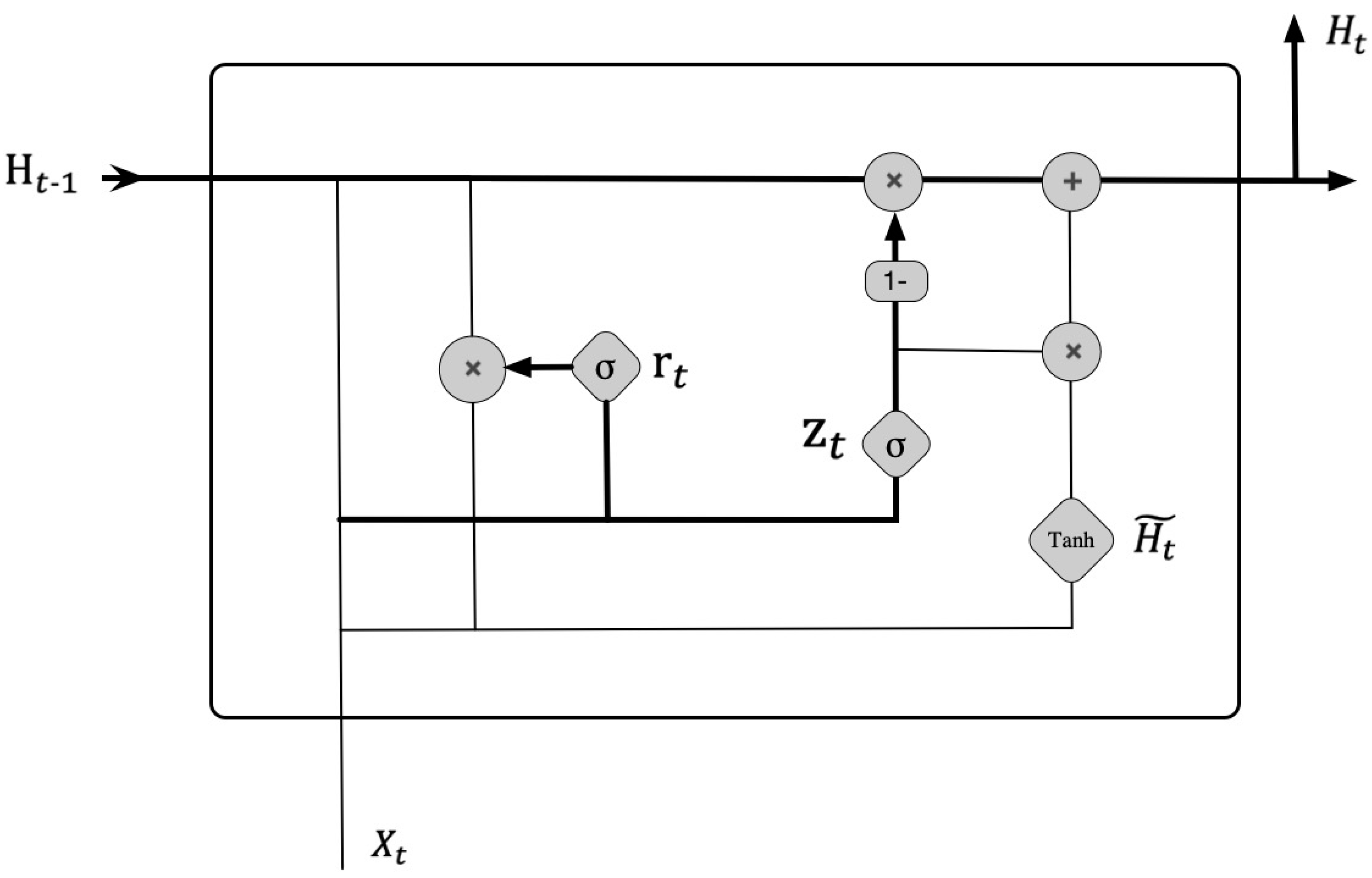
The gated-recurrent-unit network model is a neural network model that combines the unit state and hidden layer state of the long short-term memory (LSTM) [37]. The network model could improve on the shortcomings of LSTM, i.e., long training time, high number of parameters, and complex internal calculation. The GRU combines the forget gate and input gate into a single update gate and has a reset gate. By combining the cell state and hidden state, the GRU is a new method of calculating new information at the current moment based on LSTM that is different from LSTM but maintains the effect of the LSTM model. However, it has a simpler structure, fewer parameters, and a better convergence model. The basic unit structure of the gated recurrent neural network is shown in Figure 1.
In the figure, "×" and "+" represent matrix multiplication and matrix addition, respectively; σ and Tanh are the Sigmoid activation function and Tanh activation function, respectively; is the reset gate; is the update gate; is the candidate hidden state; and are the hidden state; and denotes the input.
As seen in Figure 1, the GRU has only two gates, namely the update gate and the reset gate . The update gate is used to control the degree to which the state information of the previous moment is brought into the current state. When the update gate is larger, more state information of the previous moment is brought into the current state. The reset gate is used to control the degree to which the state information of the previous moment is ignored. The smaller the value of the reset gate is, the more the state information is ignored. Through the mechanism of these two gates, the GRU can adjust the flow of information to reduce short-term memory problems. Therefore, this paper proposes an air-quality-prediction method based on the GRU to achieve long-term and continuous data prediction.
The activation functions Sigmoid and Tanh are used in the GRU to process the input values. The Sigmoid function is used to convert the input value to 0~1, as shown in Formula (1).
The Tanh function is similar to the Sigmoid function, converting the input value to between −1 and 1 and retaining a nonlinear monotonic relationship between the input and output, as shown in Formula (2).
In this paper, the number of hidden units in the GRU network is h, and the number of hidden layers is denoted by L. At a given time step t, the input is , whose batch size is n, and the sample number of each batch is d.
The steps of GRU forward propagation are as follows.
First of all, the hidden state of the last time step is . The calculations of the reset gate and update gate are shown in Formulas (3) and (4), respectively.
where are the weight matrix; are the bias matrix; and , , and are the parameters that must be updated.
In addition, the candidate hidden state is computed by the reset gate , where represents element-wise multiplication, as shown in Formula (5):
where and are the weight matrices, and is a bias matrix.
Finally, the hidden state is computed by the result of the reset gate, update gate, and candidate hidden state , as shown in Formula (6):
2.2. Genetic Algorithm
The genetic algorithm is an optimized algorithm based on the mechanism of natural selection and population inheritance. It simulates reproduction, hybridization, and mutation in the process of natural selection and inheritance and uses these bioinspired operators to generate effective solutions to optimization and search problems [38,39,40,41]. When using the genetic algorithm to solve a problem, individuals constitute every possible solution of the problem which could be encoded as a "chromosome", and the population is the solution domain, which is composed of all possible individuals. Evidently, a typical genetic algorithm generally needs to consider two prerequisites, namely the genetic representation of the solution domain and the design of the fitness function to evaluate the competitiveness of each candidate—e.g., the traveling salesman problem [42] aiming to find the optimal Hamiltonian path of the N-node graph, whose fitness function is the total cost of the path, and each feasible solution is represented as {1,2,…,N}.
The genetic algorithm starts by randomly producing individuals; the fitness value of each individual is given by being evaluated according to a predetermined fitness function, and some individuals are selected to produce the next generation based on this fitness value. Selection allows us to keep the strong ones and eliminate the weak ones. The selected individuals then produce a new generation through crossover and mutation operators, and the method of mutation and crossover varies from case to case, usually based on the properties of the particular problem. The individuals in the new generation inherit some of the good traits of the previous generation, and their performance is therefore better than that of the previous generation, thus gradually evolving towards the optimal solution. Therefore, some previous work applied the genetic algorithm to explore efficient neural network architecture [43,44,45,46,47,48].
3. The Proposed Method
This section illustrates the data preprocessing before the air-quality-prediction based on an adaptive GRU using the genetic algorithm and the GRU network structure. We also present a genetic algorithm customized for obtaining a more competitive GRU network structure. Firstly, we depict how to encode the network structure into a fixed-length binary string. Secondly, we define several genetic operations, i.e., selection, mutation, and crossover, through which we can search the adaptive GRU structure. Finally, the training and evaluation method is discussed.
3.1. Data Preprocessing
To demonstrate the data preprocessing, we have taken real-time report data of the air-quality index from 2018 to 2020 recorded at the Central Square station of Xincheng District, Xi’an as an example, which include 25,569 data points. Hourly average concentrations of fine particulate matter (PM2.5), inhalable particulate matter (PM10), sulfur dioxide (SO2), nitrogen dioxide (NO2), ozone (O3), and carbon monoxide (CO) selected from 2018 to 2020 are used as an original dataset, which is denoted by . Several parts of dataset are shown in Table 1.
The original dataset is divided into a training set , a validation set , and a testing set , which are based on a certain proportion mentioned in the following section. Then, the normalization operation is applied to the three sets to balance the influence of different types of air pollutants on the fitness. Taking the training set as an example, the method of normalization is shown in Formula (7).
Here, represents the data in ; ; n is the number of training samples; is the mean of data in ; is the standard deviation of data in ; and represents the data of which is normalized from .
The dataset is shown in Table 2.
Then, each continuous 25 h of the normalized dataset is represented as a sample. The previous 24 h (i.e., the data in order 0–23 h) of the sample will serve as the input, and the last hour (i.e., the data in order 24 h) denotes the label of the input data; this operation will work in the training set, validation set, and testing set. The sample is shown in Table 3.
3.2. The Network Structure of GRU
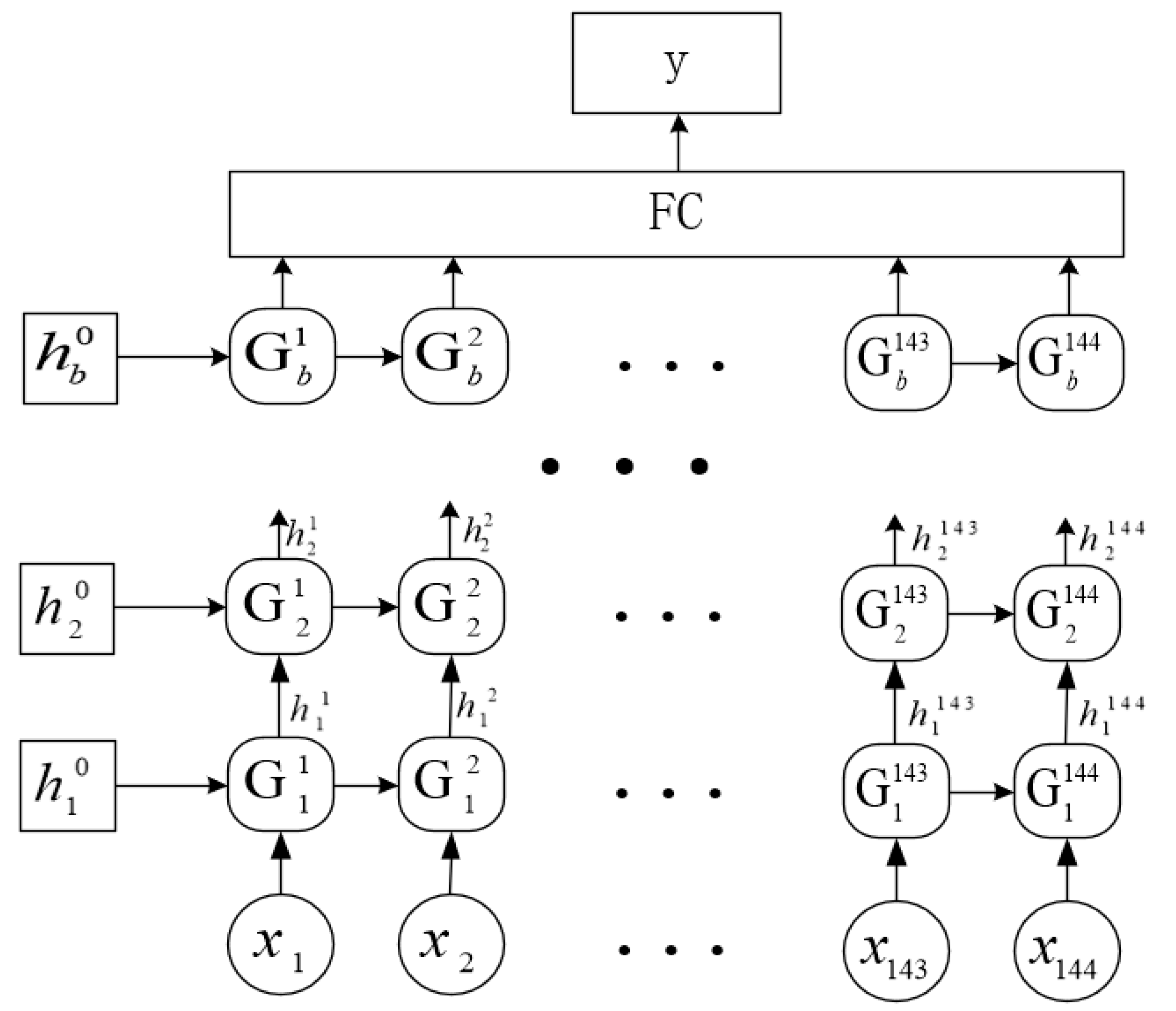
In this paper, we use the genetic algorithm to search the solution domain of the GRU network structures, and the best solution in this paper includes a feature in the hidden state and b hidden layers; its network structure is shown in Figure 2. is the input of the network with B batch size, where 144 is the number of data points of 6 air pollutants in 24 h, and the nth element of x is denoted as . represents the mth structural unit of the lth layer of the network. denotes the output of , while is the initial hidden state of the lth layer. The fully connected network is denoted as FC. A schematic diagram of the proposed GRU neural networks is shown in Figure 2.
3.3. Binary-Network Representation
We provide a binary-string representation for a network structure. We firstly note that the number of layers and the number of features in hidden state is variable, which mainly affect the effectiveness of the GRU, while the size of input and output data is unchanged after being defined.
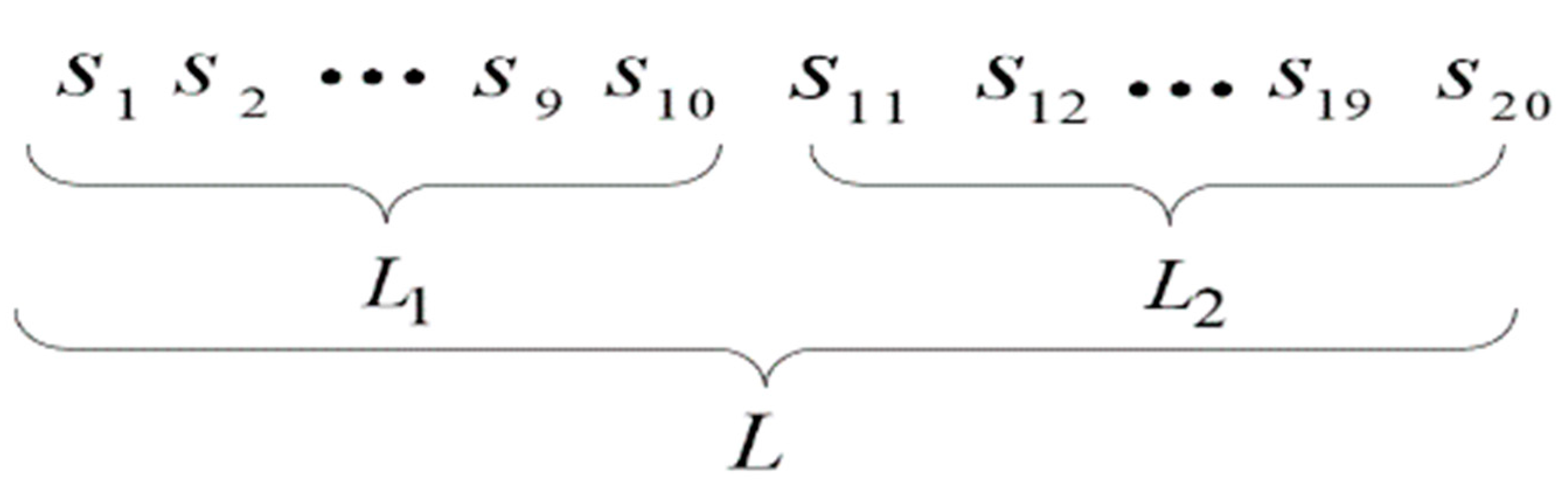
In this paper, we use a binary string of length 20 as an example. Figure 3 shows the binary string with random numbers that may occur in our experiment.
Here, the i-th number of the string is , i = 1,2,…,20. The first 10 numbers of the string represent the code of the number of layers , which is denoted as ; the remaining numbers represent the number of features in the hidden state , which is denoted as .
decodes to the solution as shown in Formula (7).
Similarly, decodes to the solution as shown in Formula (8).
Here, we take as an example, where and . The final numbers of layers and features are 55 and 2, respectively.
3.4. Genetic Operation
The genetic algorithm starts with the initialization of N random individuals. We perform T generations of the whole genetic process—i.e., we repeat the operations of selection, crossover, and mutation T times. Then, the fitness of each individual is obtained by training the reference dataset. The detailed genetic algorithm is shown in the following algorithm steps.
3.4.1. Initialization
First, we randomly initialize a group of models . The number of layers and the number of features in the hidden state of each model of the group are represented by a binary string of length 20. Each bit, , , of the binary string independently follows a Bernoulli distribution: . Then, we obtain the fitness of each initial model by the fitness function. The fitness function in this paper is shown in Formula (11).
Here, is the loss generated after evaluating the model which has pretrained on the reference dataset for the kth air pollutant.
3.4.2. Selection
We then perform selection at the beginning of each generation. At the beginning of the t-th generation, the fitness of individual at the (t − 1)th generation or initial generation is given by the fitness function. Here, affects the probability of being selected in the selection process.
Rank selection is used to determine which individuals survive the selection process. Firstly, at the beginning of generation T, the population is sorted according to fitness values. Each chromosome is then assigned selection probabilities based on its rank [43]. Individuals are selected according to their selection probability, and each individual from the previous generation can be selected multiple times in order to keep the number of individuals constant.
In rank selection, the sum of ranks is computed and the probability of each individual is computed, as shown in Formulas (10) and (11), respectively:
where denotes the jth individual of the ith layer.
3.4.3. Mutation
We give each bit of code of the a probability to change, and the individuals with the probability are selected to perform this process. In general, is very small. For example, is used in our experiment. Although the mutation may not have a great impact on the individual, its purpose is to provide new possibilities while preserving the excellent genotype of the surviving individual.
3.4.4. Crossover
Crossovers involve genotypic changes in both individuals, and denotes the number of individuals that will be selected to perform this process (Algorithm 1). The basic operated object is a stage of the genotype, rather than a single gene, with the aim of preserving the local structure of a good genotype. Similar to mutations, each pair of corresponding stages is exchanged with a small probability . In this paper, we have adopted the single-point crossover method. First, two crossover points are randomly set in the two individual coding strings that correspond with each other. Then, the two individuals swap parts of their chromosomes between the two designated intersections.
| Algorithm 1 The Genetic Process for Network |
| 1: Input: the reference dataset D, the number of generations T, the number of individuals in each generation N, the mutation probability , the crossover probabilities , the mutation parameter , and the crossover parameter . 2: Initialization: randomly generating a group of models and computing their fitness; 3: for t = 1, 2, 3,…, T do 4: Selection: generating a new generation using rank selection; 5: Crossover: performing crossover with probability and parameter ; 6: Mutation: performing mutation on each individual with probability and parameter ; 7: Evaluation: computing the fitness for each individual ; 8: end for 9: Output: the final generation . |
3.5. Training and Evaluation
For each dataset, the genetic algorithm is implemented in the training set corresponding with the dataset. In the genetic process, we set the number of generations as 100 and the number of individuals as 20; the fitness of each individual in the validation dataset is achieved after training 200 epochs, and this fitness is the evaluation index fitness. Finally, we obtain an optimal GRU network structure i.e., the GRU structure with the best fitness in all individuals at the final genetic generation.
Next, we use the adaptive network structure to train the corresponding dataset in this experiment to obtain the final optimal predicted result. The network after 1000 training iterations is obtained via the training set, and the predicted results are obtained by inputting the testing data. The predicted results will be evaluated by the evaluation index.
4. Experiments and Analysis
In order to verify the effectiveness of air-quality prediction based on adaptive GRU using genetic algorithm, the actual data of three observation stations in Xi’an city were used for the experiments. The following is an introduction to the dataset used for the experiments, the experimental environment, the experimental evaluation index, the experimental results, and analysis.
4.1. Datasets
This paper adopted the real-time air-quality information collected by the following three air-quality observatories in Xi’an city, China, as the experimental datasets: Dataset 1, Xi’an Xincheng Center Square Station from 2018 to 2020; Dataset 2, Xi’an Caotang Base; Dataset 3, Xi’an Gaoxin West Station.
The air-quality dataset of Xi‘an Xincheng Center Square Station from 2018 to 2020 includes 25,569 data points, that of Xi’an Gaoxin West Station includes 14,567 data points, and that of Xi’an Caotang base includes 14,568 data points. The quantity of data in the three datasets is shown in Table 4.
In this paper, the data from every 25 consecutive hours are considered as a sample. The data of the previous 24 h are considered as the input data, and the data of the last 1 h are considered as label data. The stride is designed as 1, and these processed datasets are made into reconstructed datasets. The sample quantity of the reconstructed datasets is shown in Table 5.
In addition, the datasets were divided into training sets and testing sets at a rate of 7:3, and the last 10% of the training set was then taken as a validation set—i.e., the first 63% of each reconstructed dataset was taken as the training set, the following 7% as the validation set, and the last 30% as the testing set.
The sample numbers in the training set, validation set, and testing set obtained from each reconstructed dataset are shown in Table 6.
4.2. The Experimental Environment
The code was run on a computer with an Intel(R) Core (TM) i9-10900K CPU @3.70 GHz, NVIDIA GeForce RTX 2080, 128 GB RAM, 1 T SSD, Python3.6, and PyTorch 1.4.1.
The number of genetic-process generations was 100. The number of iterations was set to 1000. The learning rate was 0.02. The batch size was 512. Two fully connected layers were included: the first layer had 256 hidden nodes, and the second layer had 512 hidden nodes.
4.3. The Experimental Evaluation Index
In order to evaluate the effectiveness of the air-quality-prediction model proposed in this paper, two evaluation indexes were adopted, namely root-mean-square error (RMSE) and symmetric mean absolute percentage error (SMAPE), which were used to analyze the error between the prediction results and the real data. In general, the smaller the RMSE and SMAPE values are, the smaller the deviation between the predicted results and the true values is and the better the model is. The calculation formulas of RMSE and SMAPE are shown in Equations (13) and (14), respectively.
Here, y is the prediction of the model, represents the real data taken from the real-time air-quality measurements, and m is the sum of the number of data points used in calculation.
Here, f is the prediction of the model, represents the real data taken from the real-time air-quality measurements, and n is the sum of the number of data points used in calculation.
4.4. The Adaptive GRU Structure Using Genetic Algorithm
In order to prove the efficiency of the genetic algorithm used in this paper in searching the adaptive GRU network structure, we applied the genetic algorithm process to the GRU network structure in three datasets.
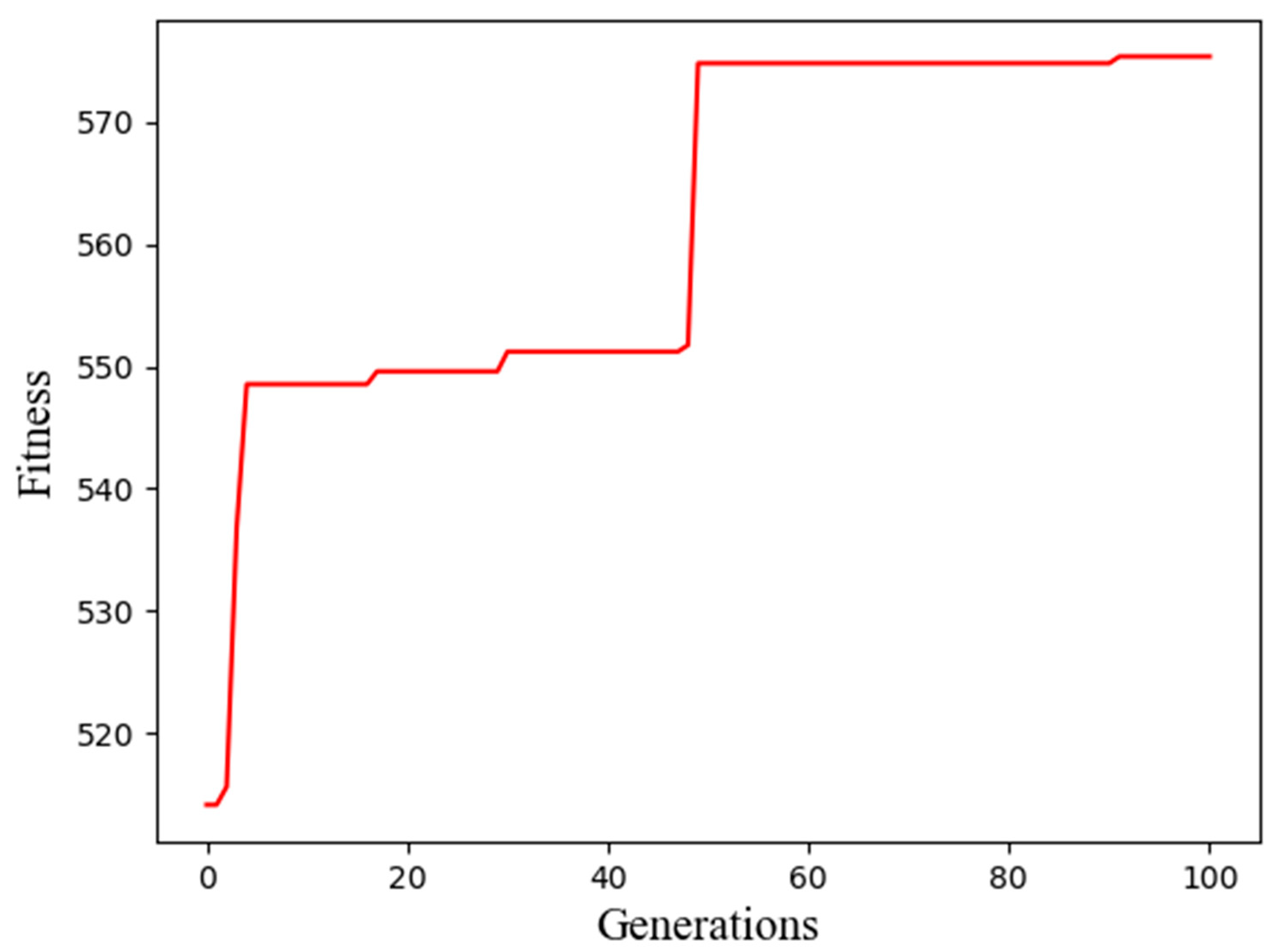
The generations and corresponding best fitness in Dataset 1 are shown in Figure 4.
The best fitness and corresponding network structure at each genetic generation are shown in Table 7.
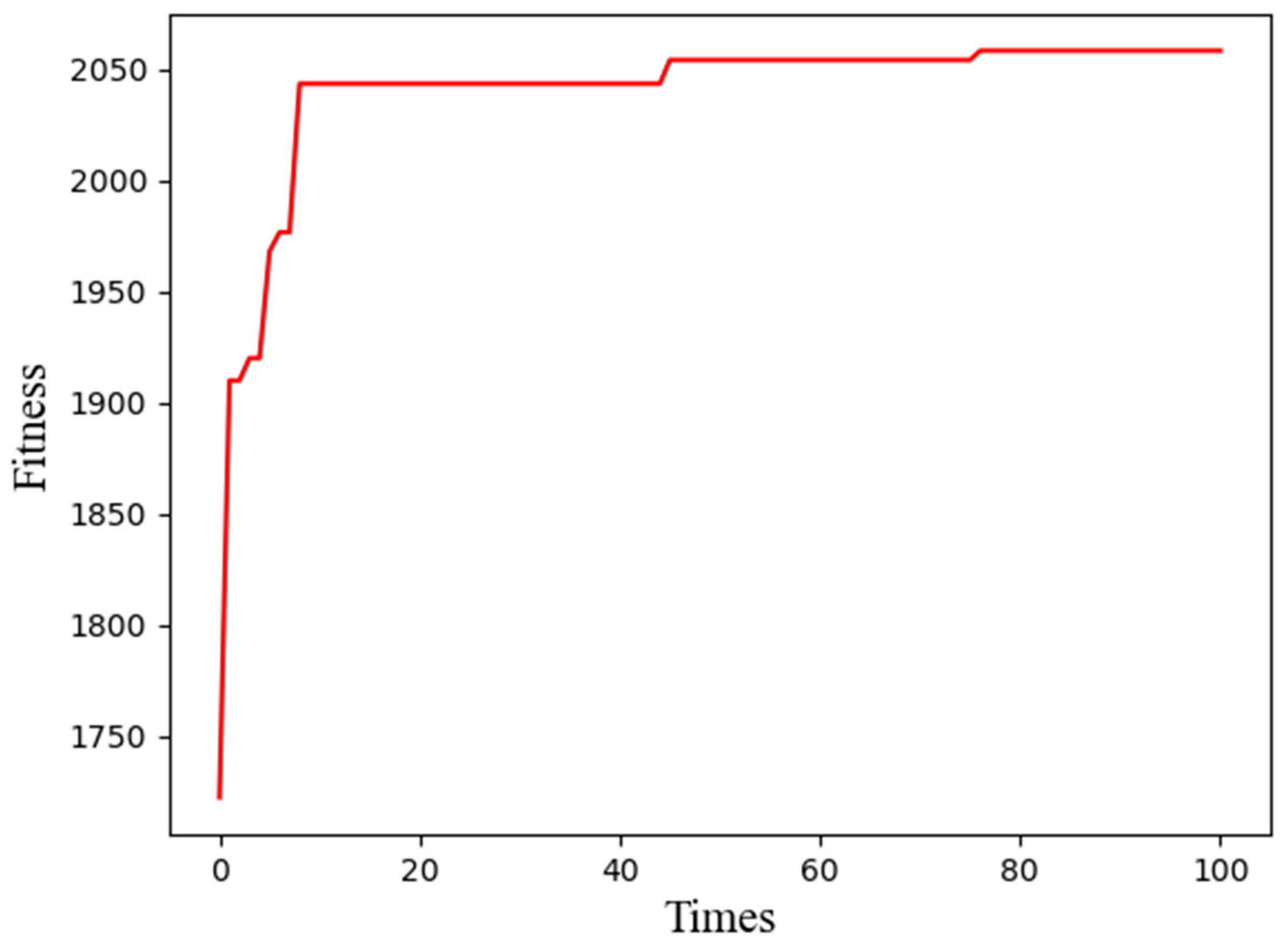
The generations and corresponding best fitness in Dataset 2 are shown in Figure 5, and the best fitness and corresponding network structure at each genetic generation are shown in Table 8.
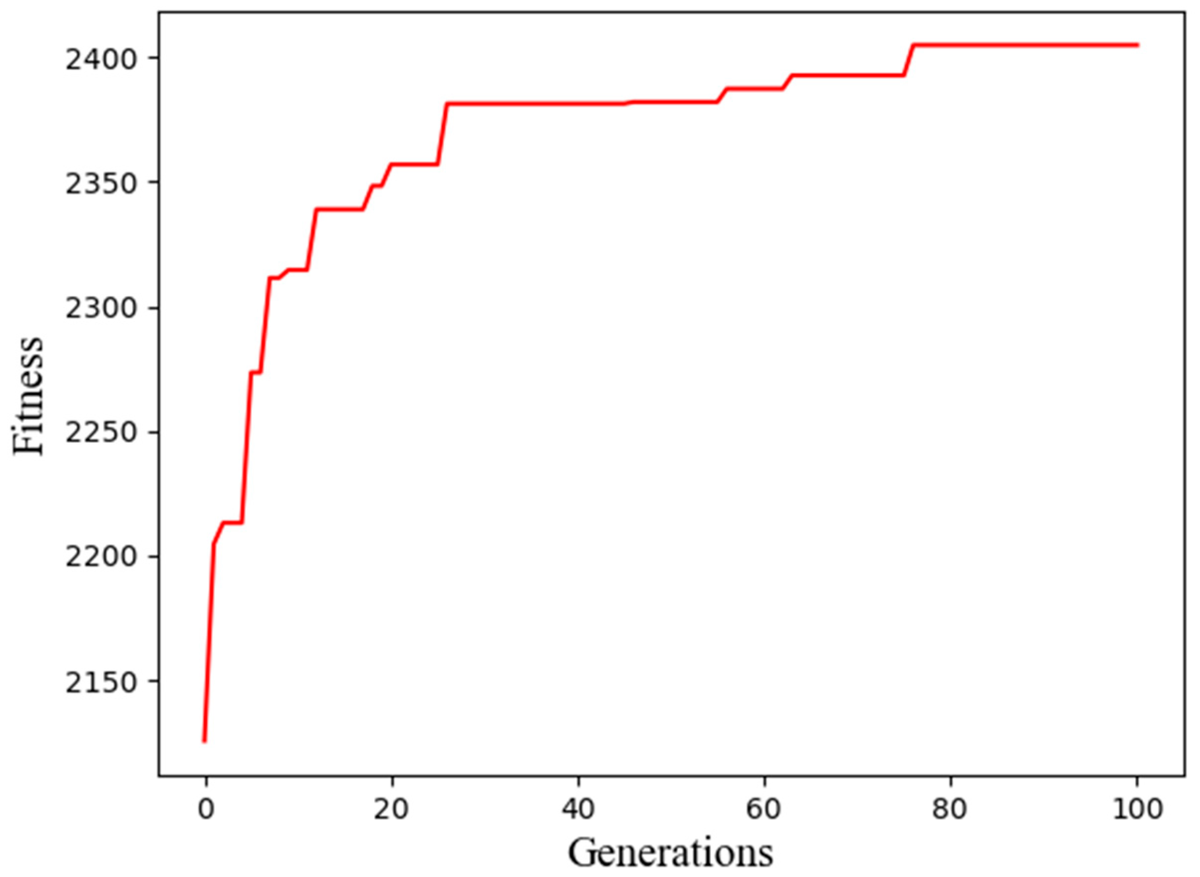
The generations and corresponding best fitness in Dataset 3 are shown in Figure 6.
The best fitness and corresponding network structure at each genetic generation are shown in Table 9.
As shown in Figure 4, Figure 5 and Figure 6, we observed, in detail, a change in the best fitness and corresponding generations.
Table 7, Table 8 and Table 9 demonstrate that the best fitness always emerges in the final generation, so the best network structure is also in the final generation. Finally, the optimal number of hidden layers of the GRU and the number of features of the GRU were 54 and 6, respectively, with Dataset 1; 55 and 2, respectively, with Dataset 2; and 61 and 2, respectively, with Dataset 3.
4.5. The Adaptive GRU Structure Compared with the Manually Designed GRU Structure
To prove the effectiveness of the adaptive GRU structure, we compared it with two manually designed structures with the three datasets. These two GRU network structures were manually designed as follows:
GRU1: 3 features in hidden state and 10 hidden layers;
GRU2: 256 features in hidden state and 256 hidden layers;
GRU_GA: the adaptive GRU structure.
The results for Dataset 1 are shown in Table 10.
As shown in Table 10, the adaptive GRU network structure obtained the best prediction results for five air pollutants. For O3, the GRU_GA structure achieved the second-best prediction results, which are almost equal to the best one.
The results for Dataset 2 are shown in Table 11.
As shown in Table 11, the adaptive GRU network structure achieved the best prediction results compared with the other two manually designed GRU network structures with Dataset 2, except for CO.
The results for Dataset 3 are shown in Table 12.
Table 12 shows that the adaptive GRU network structure performed better than the other two manually designed GRU network structures for four air pollutants in Dataset 3, and GRU1 had the best prediction results for CO and O3.
It should be noted that the adaptive GRU network structure derived from the proposed method with the three datasets could perform better than the manually designed GRU network structures for most air pollutants.
4.6. The Adaptive GRU Compared with Other Air-Quality-Prediction Methods
In order to prove the effectiveness of the proposed method in air-quality prediction, it was compared with SVM, RNN, and LSTM methods for air-quality prediction, and the prediction capability of the proposed method was verified in three datasets. The prediction results of the air-quality-prediction methods based on SVM, RNN, LSTM, and GRU_GA for each pollutant in Dataset 1 are shown in Table 13.
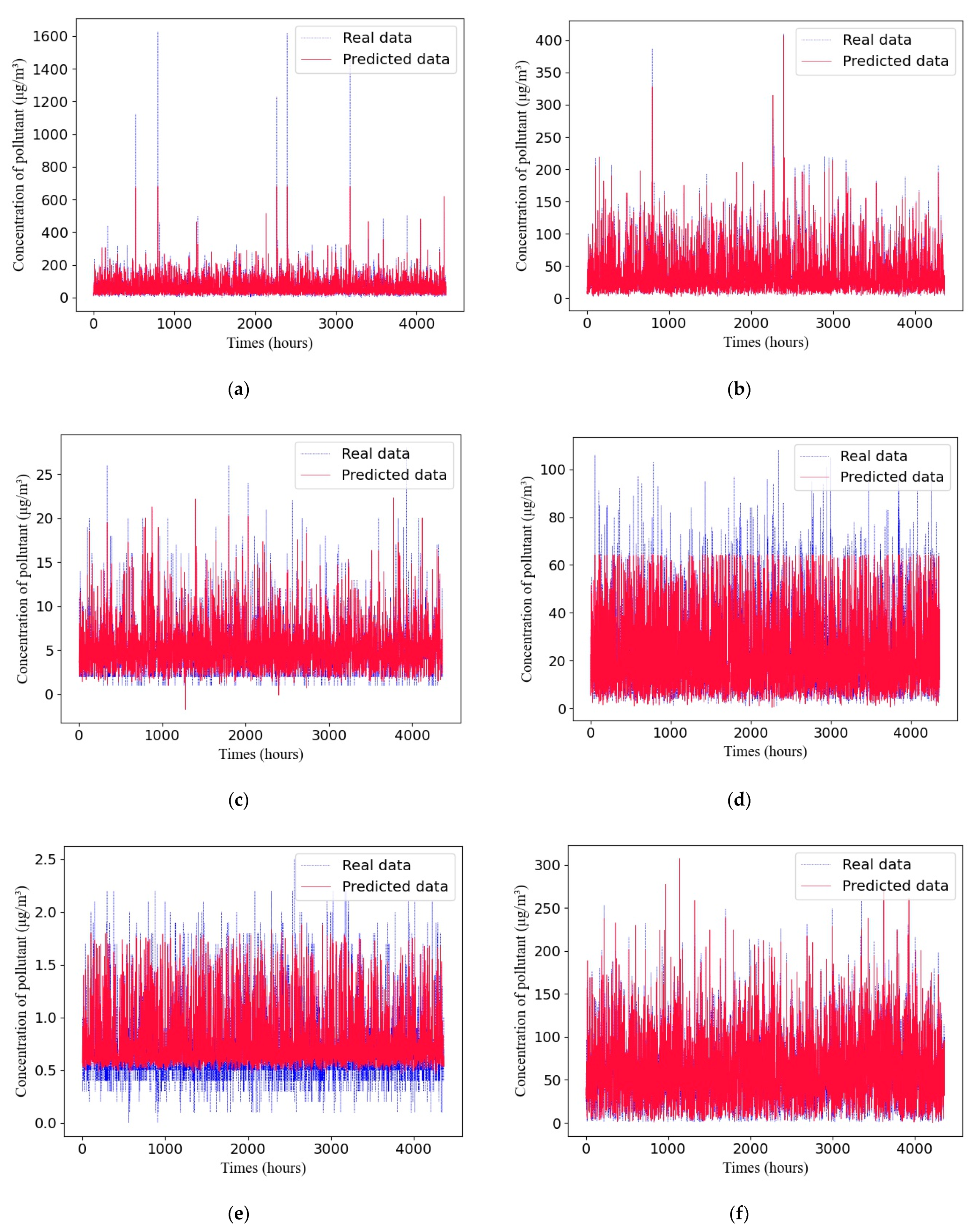
As shown in Table 13, the RMSE and SMAPE values obtained by the method proposed in this paper for the air-quality prediction of six pollutants were the best in Dataset 1, with RMSE values for PM10, PM2.5, SO2, NO2, CO, and O3 of 0.0024, 0.0078, 0.0035, 0.0068, 0.0001, and 0.0008, respectively, which are the lowest of the inferred methods. The SMAPE values with GRU_GA for PM10, PM2.5, SO2, NO2, CO, and O3 are 0.0855, 0.0678, 0.0143, 0.0959, 0.0007, and 0.0761, respectively, which are also lower than those obtained with other methods.
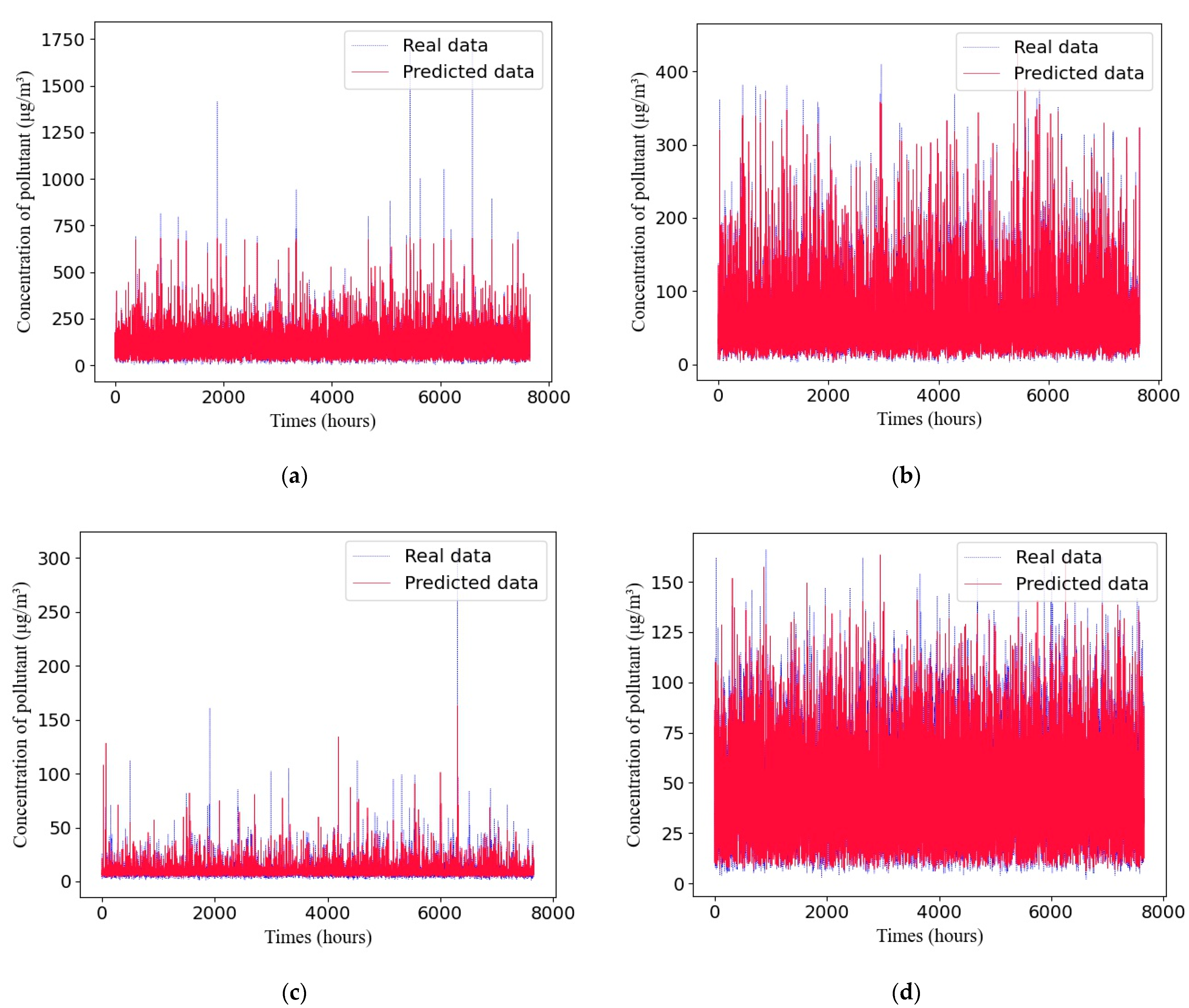
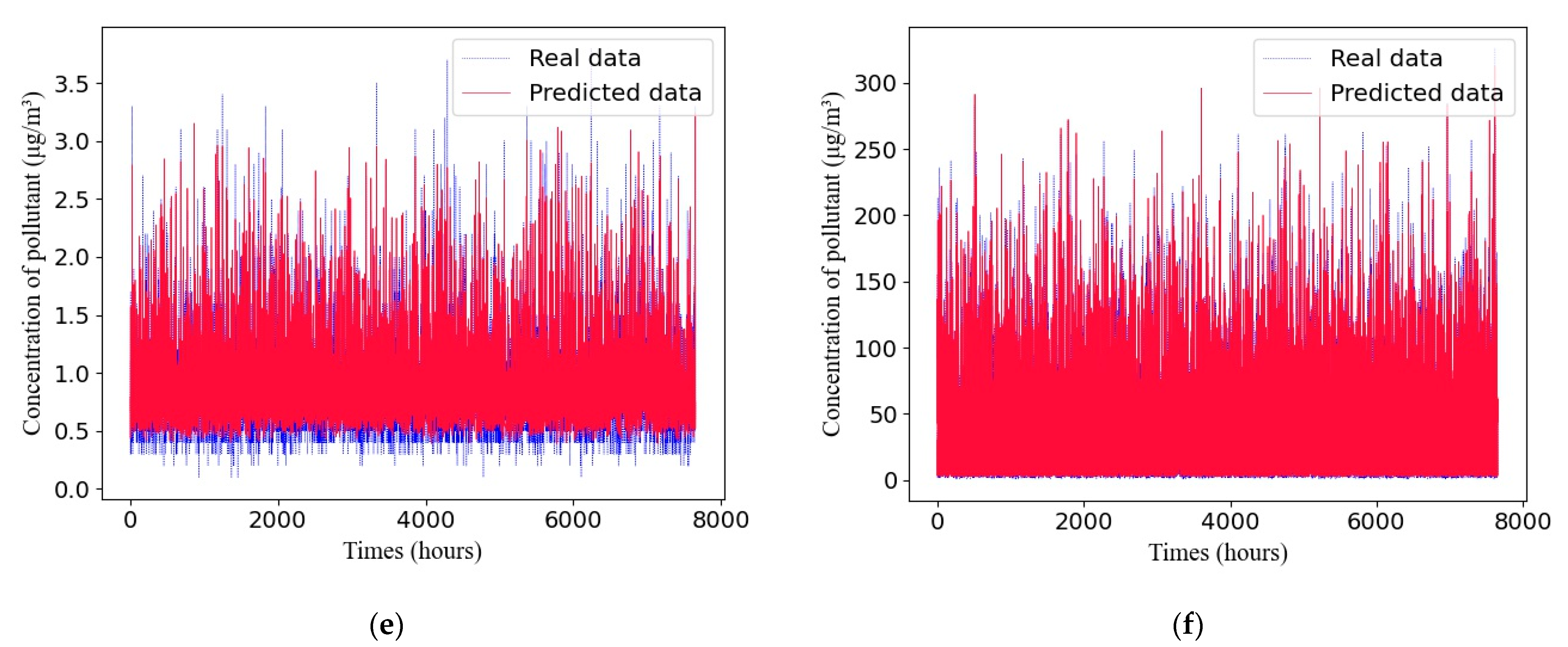
A comparison between the predicted values and true values of different pollutants with the adaptive GRU network in Dataset 1 is shown in Figure 7.
The air-quality-prediction results of SVM, RNN, LSTM, and GRU_GA for Dataset 2 are shown in Table 14.
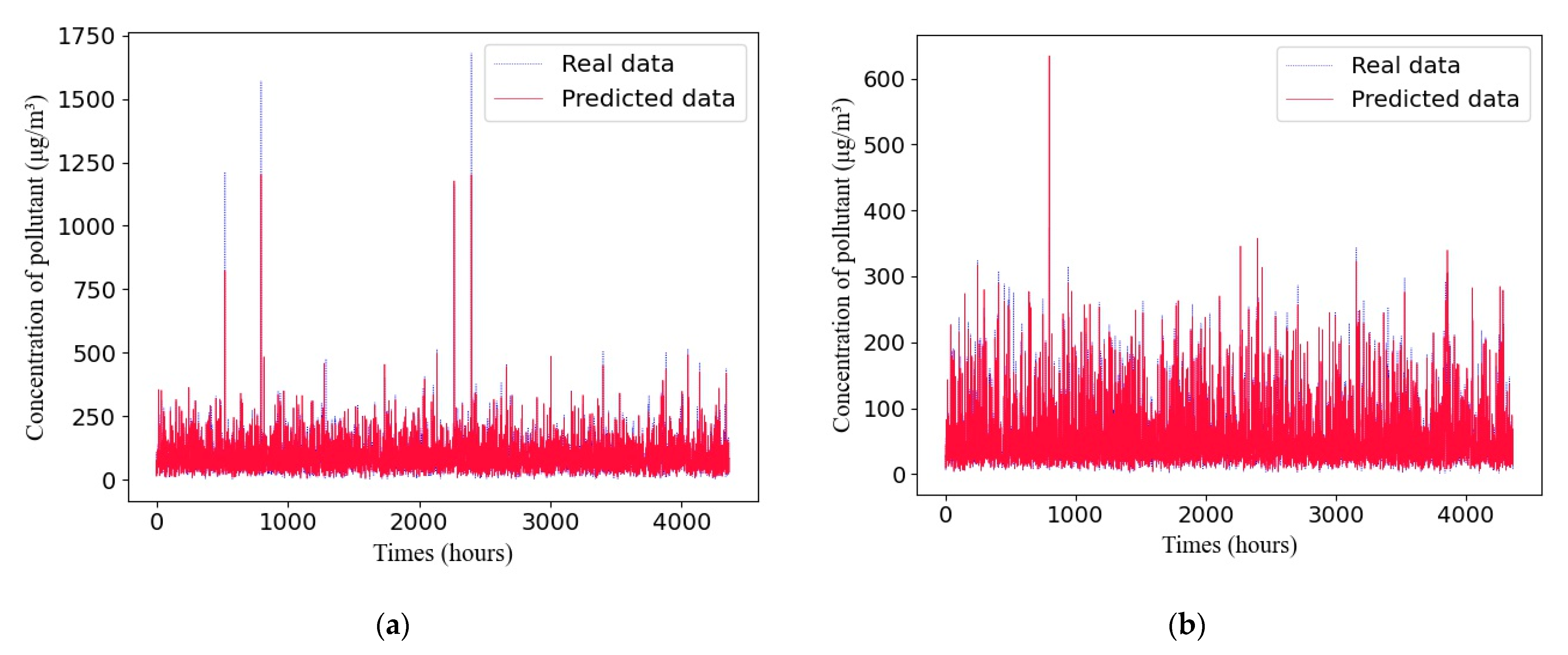
As can be seen from Table 14, GRU_GA achieved the best RMSE values for five air pollutants and the lowest SMAPE values for all pollutants in Dataset 2. The RMSE values from GRU_GA for PM10, PM2.5, SO2, NO2, and O3 were 0.0339, 0.0057, 0.0023, 0.0075, and 0.0115, respectively, which are lower than those obtained with other methods. However, the RMSE value obtained with SVM for CO was the best out of the models, at 0.0003. The SMAPE values obtained with the proposed method for the six pollutants were the best, with values for PM10, PM2.5, SO2, NO2, CO, and O3 of 0.0854, 0.0701, 0.0160, 0.0971, 0.0015, and 0.0895, respectively.
A comparison between the predicted values and true values of different pollutants from the adaptive GRU network in Dataset 2 are shown in Figure 8.
The RMSE and SMAPE values of the air-quality-prediction methods based on SVM, RNN, LSTM, and GRU for each pollutant in Dataset 3 are shown in Table 15.
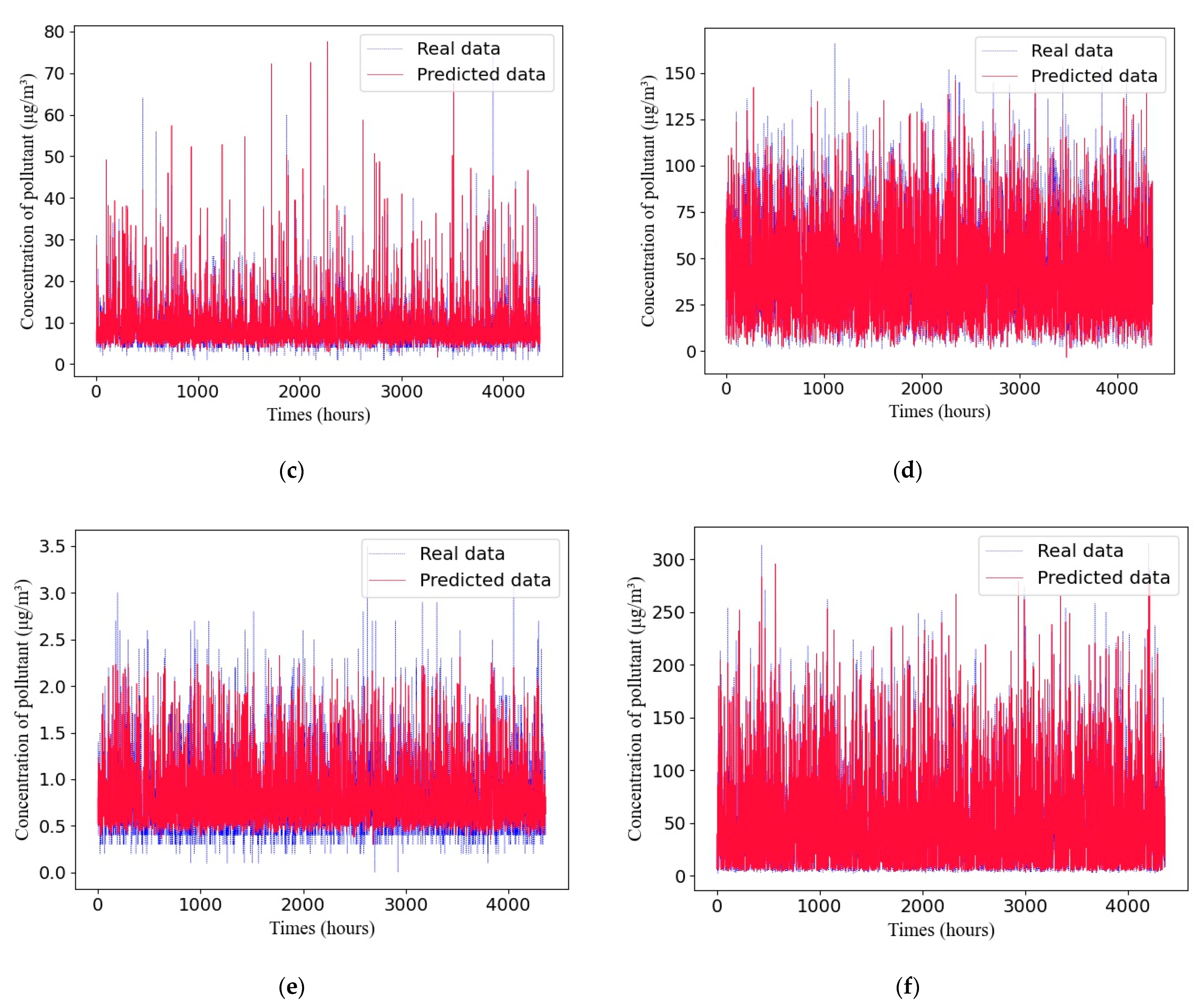
As demonstrated in Table 15, the RMSE values obtained by the GRU_GA in the air-pollutant predictions for PM10, PM2.5, SO2, NO2, and O3 were the best at 0.0208, 0.0078, 0.0028, 0.0084, and 0.0100, respectively, but compared with GRU_GA, the SVM and RNN performed better for CO with RMSE values of 0.0003. The SMAPE values with GRU_GA for the six pollutants were the best, with values for PM10, PM2.5, SO2, NO2, CO, and O3 of 0.0854, 0.0701, 0.0160, 0.0955, 0.0015, and 0.0895, respectively.
A comparison between the predicted values and true values of different pollutants with the adaptive GRU network in Dataset 3 is shown in Figure 9.
The experimental results demonstrate that air quality prediction based on the adaptive GRU using a genetic algorithm proposed in this paper is superior to that based on SVM, RNN, and LSTM methods and can obtain more accurate prediction results.
5. Conclusions
In this paper, in order to better solve air-quality data with time-sequence information, we chose a GRU to address the task of air quality prediction. Inspired by the genetic algorithm, the adaptive GRU network structure was obtained via genetic processing, and optimal prediction results of air quality were achieved. Compared with other, previously used air-quality-prediction methods, our proposed method showed a better performance in the air-quality-prediction task with three datasets. By applying the proposed method, the effective prediction of air quality can provide the government and relevant departments with the changing trend of air quality in time, which is conducive to improving the ability of environmental-protection departments to study and judge the risk information of air pollution and providing early warnings. In addition, there are many factors influencing the air quality, including not only meteorological factors but also the social environment, human factors, and the geographical environment, etc., but due to the limited data acquirement, there are insufficient data related to local production and living in Xi‘an, such as the distribution of polluting enterprises, people’s life customs, etc. Therefore, if we want to consider the effect of the whole index, a series of more detailed and effective work needs to be conducted in the later stage.
Author Contributions
Conceptualization, C.D. and Z.Z.; methodology, C.D., L.Z. and X.X.; validation, Y.Z., C.D., S.Z. and D.W; formal analysis, L.Z. and X.X.; investigation, Z.Z. and C.D.; resources, C.D. and D.W.; data curation, C.D. and Z.Z.; writing—original draft preparation, C.D. and Z.Z.; writing—review and editing, C.D., Y.Z., L.Z. and D.W; supervision, Y.Z., X.X. and L.Z.; project administration, Y.Z. and X.W.; funding acquisition, C.D., D.W. and L.Z. All authors have read and agreed to the published version of the manuscript.
Funding
This work was supported by the National Natural Science Foundations of China (grant no. 61901369, grant no. 62101454, grant no. 61834005, and grant no. 61772417), the Foundation of National Engineering Laboratory for Integrated Aero-Space-Ground-Ocean Big Data Application Technology (grant no. 20200203), and the National Key Research and Development Project of China (No. 2020AAA0104603).
Institutional Review Board Statement
Not applicable.
Informed Consent Statement
Not applicable.
Data Availability Statement
The data can only be used for research and verify the effectiveness of the method, which cannot be used for financial gain.
Acknowledgments
We acknowledge the government of Xi’an city for gathering the air-quality-pollutant information.
Conflicts of Interest
The authors declare no conflict of interest. The founding sponsors had no role in the design of the study; in the collection, analyses, or interpretation of data; in the writing of the manuscript; and in the decision to publish the results.
References
- Aliyu, Y.A.; Botai, J.O. Reviewing the local and global implications of air pollution trends in Zaria, northern Nigeria-ScienceDirect. Urban Clim. 2018, 26, 51–59. [Google Scholar] [CrossRef] [Green Version]
- Aliyu, Y.A.; Musa, I.J.; Jeb, D.N. Geostatistics of pollutant gases along high traffic points in Urban Zaria, Nigeria. Int. J. Geomat. Geosci. 2014, 5, 19–31. [Google Scholar]
- Alegria, A.; Barbera, R.; Boluda, R.; Errecalde, F.; Farré, R.; Lagarda, M.J. Environmental cadmium, lead and nickel contamination: Possible relationship between soil and vegetable content. Fresenius J. Anal. Chem. 1991, 339, 654–657. [Google Scholar] [CrossRef]
- Ercilla-Montserrat, M.; Muoz, P.; Montero, J.I.; Gabarrell, X.; Rieradevall, J. A study on air quality and heavy metals content of urban food produced in a Mediterranean city (Barcelona). J. Clean. Prod. 2018, 195, 385–395. [Google Scholar] [CrossRef]
- Wang, B.; Hong, G.; Qin, T.; Fan, W.R.; Yuan, X.C. Factors governing the willingness to pay for air pollution treatment: A case study in the Beijing-Tianjin-Hebei region. J. Clean. Prod. 2019, 235, 1304–1314. [Google Scholar] [CrossRef]
- Cohen, A.J.; Brauer, M.; Burnett, R.; Anderson, H.R.; Frostad, J.; Estep, K.; Balakrishnan, K.; Brunekreef, B.; Dandona, L.; Dandona, R.; et al. Estimates and 25-year trends of the global burden of disease attributable to ambient air pollution: An analysis of data from the Global Burden of Diseases Study 2015. Lancet 2017, 389, 1907–1918. [Google Scholar] [CrossRef] [Green Version]
- Yin, P.; He, G.; Fan, M.; Chiu, K.Y.; Fan, M.; Liu, C.; Xue, A.; Liu, T.; Pan, Y.; Mu, Q.; et al. Particulate air pollution and mortality in 38 of China’s largest cities: Time series analysis. BMJ Clin. Res. 2017, 356, j667. [Google Scholar] [CrossRef] [PubMed] [Green Version]
- United Nations. The World’s Cities in 2018 Data Booklet, 1009 Economics & Social Affairs. 2018. Available online: https://www.un.org/development/desa/pd/content/worlds-cities-2018-data-booklet (accessed on 13 April 2020).
- Afzali, A.; Rashid, M.; Afzali, M.; Younesi, V. Prediction of Air Pollutants Concentrations from Multiple Sources Using AERMOD Coupled with WRF Prognostic Model. J. Clean. Prod. 2017, 166, 1216–1225. [Google Scholar] [CrossRef]
- Todorov, V.; Dimov, I.; Ostromsky, T.; Apostolov, S.; Georgieva, R.; Dimitrov, Y.; Zlatev, Z. Advanced stochastic approaches for Sobol’ sensitivity indices evaluation. Neural Comput. Appl. 2021, 33, 1999–2014. [Google Scholar] [CrossRef]
- Dimov, I.; Todorov, V.; Sabelfeld, K. A study of highly efficient stochastic sequences for multidimensional sensitivity analysis. Monte Carlo Methods Appl. 2022, 28, 1–12. [Google Scholar] [CrossRef]
- Roeva, O.; Fidanova, S.; Paprzycki, M. Population Size Influence on the Genetic and Ant Algorithms Performance in Case of Cultivation Process Modeling. In Recent Advances in Computational Optimization. Studies in Computational Intelligence; Fidanova, S., Ed.; Springer: Cham, Switzerland, 2015; Volume 580. [Google Scholar]
- Zhou, X.; Xu, J.; Zeng, P.; Meng, X. Air pollutant concentration prediction based on GRU method. J. Phys. Conf. Ser. 2019, 1168, 032058. [Google Scholar] [CrossRef]
- Christensen, J.H. The Danish eulerian hemispheric model—A three-dimensional air pollution model used for the arctic. Atmos. Environ. 1997, 31, 4169–4191. [Google Scholar] [CrossRef]
- Zhu, J.Y.; Sun, C. Data Classification for Air Quality on Wireless Sensor Network Monitoring System Using Decision Tree Algorithm. In Proceedings of the 2016 2nd International Conference on Science and Technology-Computer (ICST), Yogyakarta, Indonesia, 27–28 October 2016. [Google Scholar]
- Kujaroentavon, K.; Kiattisin, S.; Leelasantitham, A.; Thammaboosadee, S. Air quality classification in Thailand based on decision tree. In Proceedings of the 7th 2014 Biomedical Engineering International Conference, Fukuoka, Japan, 26–28 November 2014. [Google Scholar]
- Zhang, C.; Yuan, D. Fast Fine-Grained Air Quality Index Level Prediction Using Random Forest Algorithm on Cluster Computing of Spark. In Proceedings of the 2015 IEEE 12th International Conference on Ubiquitous Intelligence and Computing and 2015 IEEE 12th International Conference on Autonomic and Trusted Computing and 2015 IEEE 15th International Conference on Scalable Computing and Communications and Its Associated Workshops (UIC-ATC-ScalCom), Beijing, China, 10–14 August 2015. [Google Scholar]
- Ghaemi, Z.; Farnaghi, M.; Alimohammadi, A. Hadoop-Based Distributed System for Online Prediction of Air Pollution Based on Support Vector Machine, The International Archives of the Photogrammetry. Remote Sens. Spat. Inf. Sci. 2015, 40, 215–219. [Google Scholar]
- Gao, S.; Hu, H.; Li, Y.; Bai, Y. Prediction of Ait Quality Index Based on MFO-SVM. J. North Univ. China Nat. Sci. Ed. 2018, 39, 373–379. [Google Scholar]
- Kingsy, R.; Grace, R.; Manimegalai, M.S.; Geetha Devasena, S.; Rajathi, K.; Usha, N.; Raabiathul, B. Air Pollution Analysis using Enhanced K-Means Clustering Algorithm for Real Time Sensor Data. In Proceedings of the IEEE Region 10 Conference, Singapore, 22–25 November 2016. [Google Scholar] [CrossRef]
- Taghavifar, H.; Mardani, A.; Mohebbi, A.; Khalilarya, S.; Jafarmadar, S. Appraisal of artificial neural networks to the emission analysis and prediction of CO2, soot, and NOx of n-heptane fueled engine. J. Clean. Prod. 2016, 112, 1729–1739. [Google Scholar] [CrossRef]
- Taylan, O. Modelling and analysis of ozone concentration by artificial intelligent techniques for estimating air quality. Atmos. Environ. 2017, 150, 356–365. [Google Scholar] [CrossRef]
- Gao, M.; Yin, L.; Ning, J. Artificial neural network model for ozone concentration estimation and Monte Carlo analysis. Atmos. Environ. 2018, 184, 129–139. [Google Scholar] [CrossRef]
- Nieto, P.; García-Gonzalo, E.; Sánchez, A.B.; Rodríguez Miranda, A.A. Air Quality Modeling Using the PSO-SVM-Based Approach, MLP Neural Network, and M5 Model Tree in the Metropolitan Area of Oviedo (Northern Spain). Environ. Model. Assess. 2018, 23, 229–247. [Google Scholar] [CrossRef]
- Gholizadeh, M.H.; Darand, M. Forecasting the Air Pollution with using Artificial Neural Networks: The Case Study; Tehran City. J. Appl. Sci. 2009, 9, 3882–3887. [Google Scholar] [CrossRef]
- Ai, H.; Shi, Y. Study on Prediction of Haze Based on BP Neural Network. Comput. Simul. 2015, 32, 402–405. [Google Scholar]
- Zhao, W.Y.; Xia, L.S.; Gao, G.K.; Cheng, L. PM2.5 prediction model based on weighted KNN-BP neural network. J. Environ. Eng. Technol. 2019, 9, 14–18. [Google Scholar]
- Ma, C.; Zu, J.; Fu, Q.; Luo, L. Air visibility forecast based on genetic neural network model. Chin. J. Environ. Eng. 2015, 9, 1905–1910. [Google Scholar]
- Li, K.; Zhou, R.; Xu, H. Based on Hopfield neural network to determine the air quality levels. In Proceedings of the 2011 International Conference on Business Management and Electronic Information, Guangzhou, China, 13–15 May 2011. [Google Scholar]
- Wang, X.; Zhang, Y.; Zhao, S.; Zhang, L. Air quality forecasting based on dynamic granular wavelet neural network. Comput. Eng. Appl. 2013, 49, 221–224. [Google Scholar]
- Fan, J.; Li, Q.; Zhu, Y.; Hou, J.; Feng, X. Aspatio-temporal prediction framework for air polution based on dep RNN. Sci. Surv. Mapp. 2017, 4, 15. [Google Scholar]
- Yang, C.; Wang, Y.; Shu, Z.; Liu, J.; Xie, N. Application of LSTM Model Based on TensorFlow in Air Quality Index Prediction. Digit. Technol. Appl. 2021, 39, 203–206. [Google Scholar]
- Li, X.; Peng, L.; Yao, X.; Cui, S.; Hu, Y.; You, C.; Chi, T. Long short-term memory neural network for air pollutant concentration predictions: Method development and evaluation. Environ. Pollut. 2017, 231, 997–1004. [Google Scholar] [CrossRef]
- Zhao, J.; Deng, F.; Cai, Y.; Chen, J. Long short-term memory-fully connected (LSTM-FC) neural network for PM2.5concentration prediction. Chemosphere 2019, 220, 486–492. [Google Scholar] [CrossRef]
- Lu, H.; Xie, M.; Wu, Z.; Liu, B.; Gao, Y.; Chen, G.; Li, Z. Chengyu region machine learning WRF-CMAQ PM2.5 concentration numerical air quality forecast. Acta Sci. Circumstantiae 2020, 40, 4419–4431. [Google Scholar]
- Chung, J.; Gulcehre, C.; Cho, K.H.; Bengio, Y. Empirical evaluation of gated recurrent neural networks on sequence modeling. arXiv 2014, arXiv:1412.3555. [Google Scholar]
- Hochreiter, S.; Schmidhuber, J. Long short-term memory. Neural Comput. 1997, 9, 1735–1780. [Google Scholar] [CrossRef]
- Houck, C.; Joines, J.; Kay, M. A Genetic Algorithm for Function Optimization: A Matlab Implementation; Technical Report; North Carolina State University: Raleigh, NC, USA, 2009. [Google Scholar]
- Reeves, C. A Genetic Algorithm for Flowshop Sequencing. Comput. Oper. Res. 1995, 22, 5–13. [Google Scholar] [CrossRef]
- Beasley, J.; Chu, P. A Genetic Algorithm for the Set Covering Problem. Eur. J. Oper. Res. 1996, 94, 392–404. [Google Scholar] [CrossRef]
- Deb, K.; Pratap, A.; Agarwal, S.; Meyarivan, T. A fast and elitist multiobjective genetic algorithm: Nsga-ii. IEEE Trans. Evol. Comput. 2002, 6, 182–197. [Google Scholar] [CrossRef] [Green Version]
- Grefenstette, J.; Gopal, R.; Rosmaita, B.; van Gucht, D. Genetic Algorithms for the Traveling Salesman Problem. In Proceedings of the International Conference on Genetic Algorithms and Their Applications, Pittsburg, PA, USA, 24–26 July 1985. [Google Scholar]
- Yao, X. Evolving Artificial Neural Networks. Proc. IEEE 1999, 87, 423–1447. [Google Scholar]
- Snyder, L.; Daskin, M. A Random-Key Genetic Algorithm for the Generalized Traveling Salesman Problem. Eur. J. Oper. Res. 2006, 174, 38–53. [Google Scholar] [CrossRef]
- Bayer, J.; Wierstra, D.; Togelius, J.; Schmidhuber, J. Evolving Memory Cell Structures for Sequence Learning. In Proceedings of the International Conference on Artificial Neural Networks, Limassol, Cypros, 14–17 September 2009. [Google Scholar]
- Ding, S.; Li, H.; Su, C.; Yu, J.; Jin, F. Evolutionary Artificial Neural Networks: A Review. Artif. Intell. Rev. 2013, 39, 251–260. [Google Scholar] [CrossRef]
- Xie, L.; Yuille, A. Genetic CNN. In Proceedings of the 2017 IEEE International Conference on Computer Vision (ICCV), IEEE Computer Society, Venice, Italy, 22–29 October 2017. [Google Scholar]
- Baker, J.E. Adaptive selection methods for genetic algorithms. In Proceedings of the International Conference on Genetic Algorithms and Their Applications, Pittsburg, PA, USA, 24–26 July 1985; pp. 101–111. [Google Scholar]
Figure 1.
The basic unit structure of the gated recurrent neural network.

Figure 2.
Schematic diagram of the proposed GRU neural networks.

Figure 3.
Example of a binary string for the network architecture.

Figure 4.
The generations and corresponding best fitness in Dataset 1.

Figure 5.
The generations and corresponding best fitness in Dataset 2.

Figure 6.
The generations and corresponding best fitness in Dataset 3.

Figure 7.
Comparison of the predicted values and real values of different pollutants with the GRU network in Dataset 1: (a) PM10; (b) PM2.5; (c) SO2; (d) NO2; (e) CO; (f) O3.
Figure 7.
Comparison of the predicted values and real values of different pollutants with the GRU network in Dataset 1: (a) PM10; (b) PM2.5; (c) SO2; (d) NO2; (e) CO; (f) O3.


Figure 8.
Comparison of predicted values and real values of different pollutants with the GRU network in Dataset 2: (a) PM10; (b) PM2.5; (c) SO2; (d) NO2; (e) CO; (f) O3.
Figure 8.
Comparison of predicted values and real values of different pollutants with the GRU network in Dataset 2: (a) PM10; (b) PM2.5; (c) SO2; (d) NO2; (e) CO; (f) O3.

Figure 9.
Comparison of the predicted values and real values of different pollutants with the GRU network in Dataset 3: (a) PM10; (b) PM2.5; (c) SO2; (d) NO2; (e) CO; (f) O3.
Figure 9.
Comparison of the predicted values and real values of different pollutants with the GRU network in Dataset 3: (a) PM10; (b) PM2.5; (c) SO2; (d) NO2; (e) CO; (f) O3.


Table 1.
Air-pollutant-data examples at the station of Xincheng Central Square in Xi’an from 2018 to 2020.
Table 1.
Air-pollutant-data examples at the station of Xincheng Central Square in Xi’an from 2018 to 2020.
| Time | PM10 (μg/m3) | PM2.5 (μg/m3) | SO2 (μg/m3) | NO2 (μg/m3) | CO (mg/m3) | O3 (μg/m3) |
|---|---|---|---|---|---|---|
| 2018-01-01 01:00 | 436 | 201 | 27 | 85 | 2.2 | 5 |
| … | … | … | … | … | … | … |
| 2020-12-31 23:00 | 267 | 218 | 21 | 82 | 2.4 | 7 |
Table 2.
The examples of the dataset .
| Order | Time | PM10 | PM2.5 | SO2 | NO2 | CO | O3 |
|---|---|---|---|---|---|---|---|
| 0 | 2018-01-01 01:00 | 5.6161 | 2.1780 | −0.3676 | 0.4809 | −0.7304 | −0.6894 |
| 1 | 2018-01-01 02:00 | 5.1333 | 3.0558 | −0.4115 | 0.3639 | −0.7260 | −0.6748 |
| … | … | … | … | … | … | … | … |
| 26,276 | 2020-12-31 23:00 | 3.1436 | 2.4267 | −0.4553 | 0.4370 | −0.7275 | −0.6602 |
Table 3.
The example of the sample.
| Order | Time | PM10 | PM2.5 | SO2 | NO2 | CO | O3 |
|---|---|---|---|---|---|---|---|
| 0 | 2018-01-01 01:00 | 5.6161 | 2.1780 | −0.3676 | 0.4809 | −0.7304 | −0.6894 |
| 1 | 2018-01-01 02:00 | 5.1333 | 3.0558 | −0.4115 | 0.3639 | −0.7260 | −0.6748 |
| … | … | … | … | … | … | … | … |
| 23 | 2018-01-02 00:00 | 6.1428 | 3.3777 | −0.0457 | 0.8613 | −0.7158 | −0.6894 |
| 24 | 2018-01-02 01:00 | 6.7573 | 5.3528 | −0.1774 | 0.7589 | −0.7099 | −0.6309 |
Table 4.
The quantity of data in three datasets.
| Dataset Name | Xi‘an Xincheng Center Square Station | Xi‘an Caotang Base | Xi‘an Gaoxin West Station |
|---|---|---|---|
| Dataset Number | Dataset 1 | Dataset 2 | Dataset 3 |
| Data Quantity | 25,569 | 14,567 | 14,568 |
Table 5.
The quantity of samples in the reconstructed datasets.
| Dataset Name | Xi‘an Xincheng Center Square Station | Xi‘an Caotang Base | Xi‘an Gaoxin West Station |
|---|---|---|---|
| Dataset Number | Dataset 1 | Dataset 2 | Dataset 3 |
| Sample Quantity | 25,545 | 14,543 | 14,544 |
Table 6.
Number of samples in training set, validation set, and testing set of the reconstructed datasets.
Table 6.
Number of samples in training set, validation set, and testing set of the reconstructed datasets.
| Dataset | Number of Samples | ||
|---|---|---|---|
| Training Set | Validation Set | Testing Set | |
| Dataset 1 | 16,093 | 1788 | 7664 |
| Dataset 2 | 9157 | 1017 | 4360 |
| Dataset 3 | 9157 | 1018 | 4360 |
Table 7.
The best fitness and corresponding network structure in Dataset 1.
| Generations | Best Fitness | Network Structure |
|---|---|---|
| 00 | 514.13 | 0110011000|0001001001 |
| 01 | 514.13 | 0110011000|0001001001 |
| 03 | 536.76 | 0110011100|0001001001 |
| 05 | 548.55 | 0110011101|0000101001 |
| 08 | 548.55 | 0110011101|0000101001 |
| 10 | 548.55 | 0110011101|0000101001 |
| 30 | 551.22 | 0111011101|0000101011 |
| 50 | 574.82 | 0111100010|0000101010 |
| 80 | 574.82 | 0111100010|0000101010 |
| 100 | 575.37 | 0110110010|0000101111 |
Table 8.
The best fitness and corresponding network structure in Dataset 2.
| Generations | Best Fitness | Network Structure |
|---|---|---|
| 00 | 1722.22 | 0010111110|0000001101 |
| 01 | 1909.79 | 0101111000|0000010101 |
| 03 | 1919.86 | 0010111101|0001011110 |
| 05 | 1967.90 | 0111000111|0001011101 |
| 08 | 2043.25 | 0111110011|0000010110 |
| 10 | 2043.25 | 0111110011|0000010110 |
| 30 | 2043.25 | 0111110011|0000010110 |
| 50 | 2053.95 | 0111110111|0000010110 |
| 80 | 2058.13 | 0110110111|0000010100 |
| 100 | 2058.13 | 0110110111|0000010100 |
Table 9.
The best fitness and corresponding network structure in Dataset 3.
| Generations | Best Fitness | Network Structure |
|---|---|---|
| 00 | 2125.73 | 0010111000|0001000010 |
| 01 | 2204.67 | 0011101111|0000101111 |
| 03 | 2213.15 | 0010010110|0000110010 |
| 05 | 2273.15 | 0011101011|0000101011 |
| 08 | 2311.43 | 0011101011|0000100001 |
| 10 | 2311.43 | 0110010110|0000101001 |
| 30 | 2381.33 | 0111011101|0000100010 |
| 50 | 2382.01 | 0111110011|0000011010 |
| 80 | 2404.84 | 0111100111|0000011011 |
| 100 | 2404.84 | 0111100111|0000011011 |
Table 10.
The result of the adaptive GRU network structure compared with manually designed GRU network structures with Dataset 1.
Table 10.
The result of the adaptive GRU network structure compared with manually designed GRU network structures with Dataset 1.
| Air Pollutant | RMSE | SMAPE | ||||
|---|---|---|---|---|---|---|
| GRU1 | GRU2 | GRU_GA | GRU1 | GRU2 | GRU_GA | |
| PM10 | 0.0264 | 0.0647 | 0.0224 | 0.0870 | 0.1937 | 0.0855 |
| PM2.5 | 0.0136 | 0.0392 | 0.0078 | 0.0699 | 0.3041 | 0.0678 |
| SO2 | 0.0067 | 0.0065 | 0.0035 | 0.0154 | 0.2734 | 0.0143 |
| NO2 | 0.0076 | 0.0202 | 0.0068 | 0.0974 | 0.3835 | 0.0959 |
| CO | 0.0088 | 0.0003 | 0.0001 | 0.0007 | 0.0014 | 0.0007 |
| O3 | 0.0087 | 0.0359 | 0.0088 | 0.0759 | 0.3608 | 0.0761 |
Table 11.
The result of the adaptive GRU network structure compared with manually designed GRU network structures with Dataset 2.
Table 11.
The result of the adaptive GRU network structure compared with manually designed GRU network structures with Dataset 2.
| Air Pollutant | RMSE | SMAPE | ||||
|---|---|---|---|---|---|---|
| GRU1 | GRU2 | GRU_GA | GRU1 | GRU2 | GRU_GA | |
| PM10 | 0.0388 | 0.0722 | 0.0339 | 0.1286 | 0.2307 | 0.1297 |
| PM2.5 | 0.0066 | 0.0330 | 0.0057 | 0.0777 | 0.3650 | 0.0692 |
| SO2 | 0.0025 | 0.0029 | 0.0023 | 0.0136 | 0.0150 | 0.0127 |
| NO2 | 0.0078 | 0.0186 | 0.0075 | 0.1045 | 0.2195 | 0.1035 |
| CO | 0.0004 | 0.0003 | 0.0004 | 0.0020 | 0.0016 | 0.0022 |
| O3 | 0.0119 | 0.0441 | 0.0115 | 0.1003 | 0.2164 | 0.0978 |
Table 12.
The result of the adaptive GRU network structure compared with manually designed GRU network structures with Dataset 3.
Table 12.
The result of the adaptive GRU network structure compared with manually designed GRU network structures with Dataset 3.
| Air Pollutant | RMSE | SMAPE | ||||
|---|---|---|---|---|---|---|
| GRU1 | GRU2 | GRU_GA | GRU1 | GRU2 | GRU_GA | |
| PM10 | 0.0273 | 0.0652 | 0.0208 | 0.0865 | 0.2136 | 0.0854 |
| PM2.5 | 0.0085 | 0.0425 | 0.0078 | 0.0740 | 0.3270 | 0.0701 |
| SO2 | 0.0045 | 0.0054 | 0.0028 | 0.0195 | 0.0285 | 0.0160 |
| NO2 | 0.0082 | 0.0246 | 0.0084 | 0.1035 | 0.3859 | 0.0971 |
| CO | 0.0003 | 0.0003 | 0.0022 | 0.0014 | 0.0016 | 0.0015 |
| O3 | 0.0099 | 0.0430 | 0.0100 | 0.0874 | 0.3124 | 0.0895 |
Table 13.
The prediction results of GRU_GA compared with other air-quality-prediction methods with Dataset 1.
Table 13.
The prediction results of GRU_GA compared with other air-quality-prediction methods with Dataset 1.
| Air Pollutant | RMSE | SMAPE | ||||||
|---|---|---|---|---|---|---|---|---|
| SVM | RNN | LSTM | GRU_GA | SVM | RNN | LSTM | GRU_GA | |
| PM10 | 0.6732 | 0.6471 | 0.6470 | 0.0224 | 0.1936 | 0.1937 | 0.1837 | 0.0855 |
| PM2.5 | 0.4031 | 0.3923 | 0.3921 | 0.0078 | 0.3031 | 0.3063 | 0.3041 | 0.0678 |
| SO2 | 0.0078 | 0.0066 | 0.0065 | 0.0035 | 0.0290 | 0.0285 | 0.0285 | 0.0143 |
| NO2 | 0.0215 | 0.0203 | 0.0202 | 0.0068 | 0.3711 | 0.3725 | 0.3617 | 0.0959 |
| CO | 0.0003 | 0.0003 | 0.0003 | 0.0001 | 0.0015 | 0.0012 | 0.0014 | 0.0007 |
| O3 | 0.0355 | 0.0358 | 0.0359 | 0.0088 | 0.3727 | 0.3601 | 0.3403 | 0.0761 |
Table 14.
The prediction results of GRU_GA compared with other air-quality-prediction methods with Dataset 2.
Table 14.
The prediction results of GRU_GA compared with other air-quality-prediction methods with Dataset 2.
| Air Pollutant | RMSE | SMAPE | ||||||
|---|---|---|---|---|---|---|---|---|
| SVM | RNN | LSTM | GRU_GA | SVM | RNN | LSTM | GRU_GA | |
| PM10 | 0.0722 | 0.0722 | 0.0722 | 0.0339 | 0.2306 | 0.2306 | 0.2307 | 0.0854 |
| PM2.5 | 0.0331 | 0.0330 | 0.0330 | 0.0057 | 0.3589 | 0.3659 | 0.3650 | 0.0701 |
| SO2 | 0.0030 | 0.0029 | 0.0031 | 0.0023 | 0.0151 | 0.0150 | 0.0150 | 0.0160 |
| NO2 | 0.0186 | 0.0187 | 0.0186 | 0.0075 | 0.2192 | 0.2341 | 0.2195 | 0.0971 |
| CO | 0.0003 | 0.0004 | 0.0007 | 0.0004 | 0.0016 | 0.0033 | 0.0016 | 0.0015 |
| O3 | 0.0440 | 0.0441 | 0.0441 | 0.0115 | 0.2167 | 0.2173 | 0.2164 | 0.0895 |
Table 15.
The prediction results of GRU_GA compared with other air-quality-prediction methods with Dataset 3.
Table 15.
The prediction results of GRU_GA compared with other air-quality-prediction methods with Dataset 3.
| Air Pollutant | RMSE | SMAPE | ||||||
|---|---|---|---|---|---|---|---|---|
| SVM | RNN | LSTM | GRU_GA | SVM | RNN | LSTM | GRU_GA | |
| PM10 | 0.0651 | 0.0651 | 0.0652 | 0.0208 | 0.2130 | 0.2128 | 0.2133 | 0.0854 |
| PM2.5 | 0.0425 | 0.0425 | 0.0425 | 0.0078 | 0.3260 | 0.3270 | 0.3277 | 0.0701 |
| SO2 | 0.0054 | 0.0054 | 0.0055 | 0.0028 | 0.0284 | 0.0284 | 0.0291 | 0.0160 |
| NO2 | 0.0246 | 0.0246 | 0.0247 | 0.0084 | 0.1673 | 0.1681 | 0.2837 | 0.0955 |
| CO | 0.0003 | 0.0003 | 0.0006 | 0.0022 | 0.0016 | 0.0016 | 0.0028 | 0.0015 |
| O3 | 0.0430 | 0.0430 | 0.0431 | 0.0100 | 0.3132 | 0.3139 | 0.3150 | 0.0895 |
Publisher’s Note: MDPI stays neutral with regard to jurisdictional claims in published maps and institutional affiliations. |
© 2022 by the authors. Licensee MDPI, Basel, Switzerland. This article is an open access article distributed under the terms and conditions of the Creative Commons Attribution (CC BY) license (https://creativecommons.org/licenses/by/4.0/).
Share and Cite
MDPI and ACS Style
Ding, C.; Zheng, Z.; Zheng, S.; Wang, X.; Xie, X.; Wen, D.; Zhang, L.; Zhang, Y. Accurate Air-Quality Prediction Using Genetic-Optimized Gated-Recurrent-Unit Architecture. Information 2022, 13, 223. https://doi.org/10.3390/info13050223
AMA Style
Ding C, Zheng Z, Zheng S, Wang X, Xie X, Wen D, Zhang L, Zhang Y. Accurate Air-Quality Prediction Using Genetic-Optimized Gated-Recurrent-Unit Architecture. Information. 2022; 13(5):223. https://doi.org/10.3390/info13050223
Chicago/Turabian StyleDing, Chen, Zhouyi Zheng, Sirui Zheng, Xuke Wang, Xiaoyan Xie, Dushi Wen, Lei Zhang, and Yanning Zhang. 2022. "Accurate Air-Quality Prediction Using Genetic-Optimized Gated-Recurrent-Unit Architecture" Information 13, no. 5: 223. https://doi.org/10.3390/info13050223
Note that from the first issue of 2016, this journal uses article numbers instead of page numbers. See further details here.