Abstract
Background: Distinguishing between the spinal cord and cerebrospinal fluid (CSF) non-invasively on CT is challenging due to their similar mass densities. We hypothesize that patch-based machine learning applied to dual-energy CT can accurately distinguish CSF from neural or other tissues based on the center voxel and neighboring voxels. Methods: 88 regions of interest (ROIs) from 12 patients’ dual-energy (100 and 140 kVp) lumbar spine CT exams were manually labeled by a neuroradiologist as one of 4 major tissue types (water, fat, bone, and nonspecific soft tissue). Four-class classifier convolutional neural networks were trained, validated, and tested on thousands of nonoverlapping patches extracted from 82 ROIs among 11 CT exams, with each patch representing pixel values (at low and high energies) of small, rectangular, 3D CT volumes. Different patch sizes were evaluated, ranging from 3 × 3 × 3 × 2 to 7 × 7 × 7 × 2. A final ensemble model incorporating all patch sizes was tested on patches extracted from six ROIs in a holdout patient. Results: Individual models showed overall test accuracies ranging from 99.8% for 3 × 3 × 3 × 2 patches (N = 19,423) to 98.1% for 7 × 7 × 7 × 2 patches (N = 1298). The final ensemble model showed 99.4% test classification accuracy, with sensitivities and specificities of 90% and 99.6%, respectively, for the water class and 98.6% and 100% for the soft tissue class. Conclusions: Convolutional neural networks utilizing local low-level features on dual-energy spine CT can yield accurate tissue classification and enhance the visualization of intraspinal neural tissue.
1. Introduction
Computed tomography (CT) is a commonly used modality for the evaluation of bony spine abnormalities by virtue of its widespread availability, rapid acquisition times, and depiction of fine bony detail. However, its clinical utility in assessing intraspinal soft tissue abnormalities is limited. Cord compression, disc herniations, or intraspinal soft tissue tumors can be missed on CT, even by experienced radiologists, because they are often inconspicuous or invisible on CT [1,2]. Magnetic resonance imaging (MRI) offers superior intraspinal soft tissue and fluid depiction but is not always readily available or feasible, often due to contraindications or patient aversions to MRI, such as claustrophobia, body habitus, metallic implants, etc. [3,4]. Myelography, in which extrinsic iodinated contrast material is injected into the spinal canal, permits high-resolution imaging of the spinal cord and nerve roots [5] but is invasive and is much more time-consuming than CT. In some cases, myelography is not possible due to the limited tolerance of prone positioning, bleeding concerns, or other procedural contraindications. Therefore, there is a clinical need for alternative approaches to augment spinal cord visualization accurately and robustly on routine spine CT.
Conventional CT relies on differences in X-ray attenuation among different tissue types based on atomic number, mass density, or uptake of extrinsic contrast agents. However, within the spinal canal, the ability to discern the spinal cord from surrounding cerebrospinal fluid (CSF) is markedly limited due to the high overlap in attenuation values between the spinal cord and CSF, rendering CT unreliable for visualization of the spinal cord in most practical settings. Dual-energy CT post-processing techniques can improve the specificity of differentiation among tissue types [6], but routinely used segmentation methods based on material decomposition typically require a sufficiently large atomic number difference that is not present between the spinal cord and CSF. Dual-energy post-processing techniques have been shown to be helpful in reducing artifacts from metallic hardware [7,8,9], but even in the absence of metallic hardware, beam-hardening artifacts and noise related to photon attenuation by the bony spinal elements result in wide variations in pixel values that further hinder attempts to differentiate between spinal cord and CSF on CT. Differential uptake of extrinsic iodinated contrast material can assist in segmenting different tissue types in many non-neuroradiologic imaging applications, but because normal spinal cord parenchyma is separated from the vasculature by a blood–CNS barrier, contrast administration has very little utility in improving spinal cord visualization on CT.
Machine learning approaches, such as deep convolutional neural networks (CNNs), have been used to augment medical images [10,11,12], including the segmentation of medical images by tissue type. The application of deep neural networks to the automated segmentation of bony structures from soft tissue in spine CT has been reported [13,14,15]. For instance, Vania et al. used two-dimensional patches of spine CT images to create a method for segmenting the bony elements of the spine from adjacent non-bony tissues, with pixel-wise sensitivity and a specificity of 97% and 99%, respectively [13]. Another two-dimensional patch-based method was able to distinguish bone from non-bone pixels on spine CT with 91% sensitivity and 93% specificity [14]. Often favorable accuracies are achievable for this task due to the large differences in density between bone and soft tissue pixels, but none of the above studies address the more challenging task of differentiating spinal cord voxels from CSF on CT. Automated methods have also been described for detecting the general region of the spinal cord or nerve roots by their location relative to vertebral anatomy [16,17], but these methods likely rely on the pixel position relative to bony structures without attempting to differentiate neural soft tissue pixels from water pixels that may occur in these locations.
In this study, we propose a patch-based machine learning method to help differentiate major tissue types in the spine, with an emphasis on differentiating the spinal cord from CSF. We applied this to lumbar spine CT exams as the transition in intraspinal contents from the spinal cord to predominantly CSF near the thoracolumbar junction serves as a suitable site for evaluating the model’s performance. A prior study reporting improved soft-tissue visualization of spine tumors using dual-energy CT post-processing [18] lends credence to the proposition that sufficient information is contained within dual-energy CT data to differentiate among soft tissues with subtle attenuation differences on conventional CT. In this study, we test the hypothesis that machine learning-based predictive models can accurately classify small dual-energy CT patches as CSF, neural tissue (spinal cord and nerves), fat, or bone using only information from the center voxel and its immediate surrounding neighboring voxels.
2. Materials and Methods
2.1. Subjects and Source Data
Following IRB approval, we assembled a custom in-house repository of 3-dimensional (3D) regions of interest (ROIs) of dual-energy CT volumes, pooled from a retrospective cohort of 12 patients having undergone dual-energy lumbar spine CT requested for clinical reasons due to the presence of hardware within portions of the spine. Patient ages ranged from 45 to 66 years (median age: 59). All CT examinations were performed on a dual-source spiral scanner (Siemens Somatom Definition FLASH, Siemens, Erlangen, Germany) at low (100 kVp) and high (140 kVp) energies. Median tube current-time products were 281 and 212 mAs, respectively. Source images used for this study consist of 512 × 512 CT images of 0.75 mm thickness at 16-bit grayscale, obtained using an I50f reconstruction kernel. The median reconstruction diameter was 171 mm.
ROI selection was performed manually by a fellowship-trained neuroradiologist (X.V.N.) with 14 years of experience interpreting MR and CT images. Because subsequent classification was to be performed with small individual voxel patches as input data rather than using the entire volume or whole slices as input, it was not necessary to perform a full manual 3D segmentation of each CT volume. Instead, the radiologist was tasked with selecting appropriate 3D ROIs that were representative of the targeted tissue classes and had relatively uniform tissue composition, avoiding slices with metallic artifacts. Because the ROIs were to be subsequently pooled to generate the voxel patches used for machine learning, more than one ROI per CT exam per class label was permitted. The radiologist first visualized each CT examination as a stacked series of CT images with low and high-energy images represented as separate imaging channels. Using built-in functions within the open-source FIJI image-processing package [19], rectangular 3D ROIs for each dual-energy pair of CT image volumes were manually selected and identified as one of the following: bone, fat, muscle, intrabladder/intrabowel fluid, spinal cord, or CSF.
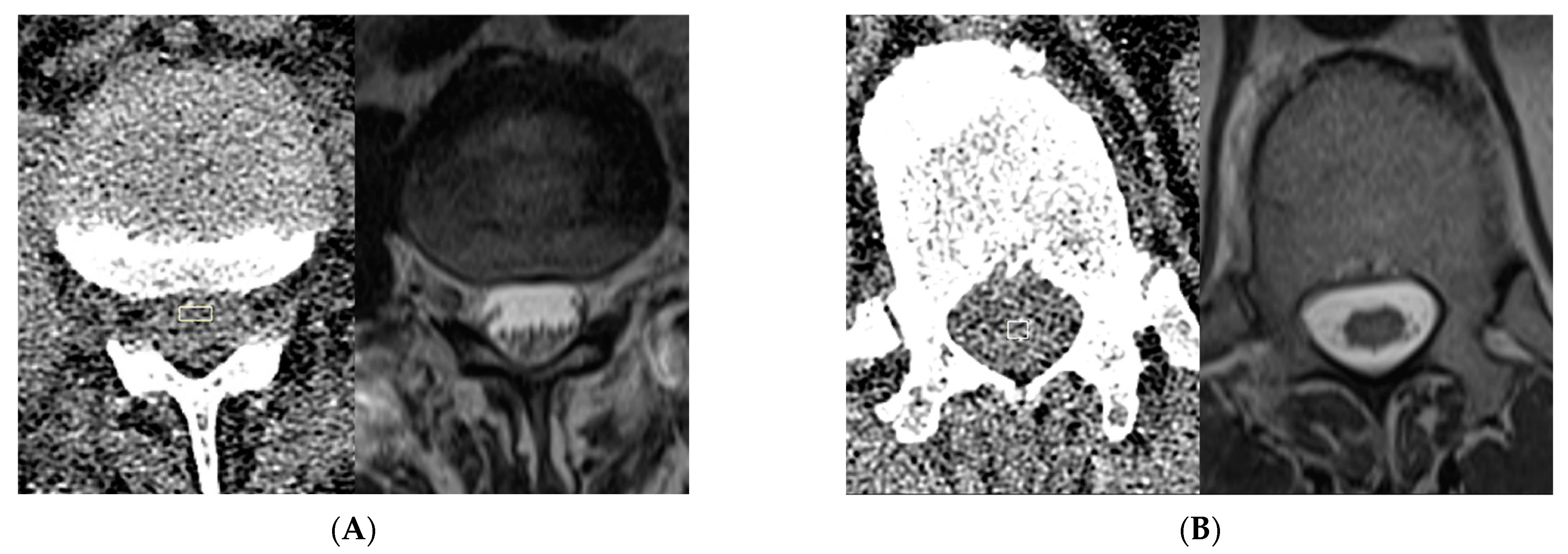
In total, 13 ROIs labeled as bone were derived from both areas of cortical and trabecular bone, 9 of which were acquired at the T12 or L1 vertebral body, and 4 of which were selected from the sacrum or iliac bones. In total, 15 ROIs labeled as fat were selected, with 12 from the dorsal subcutaneous fat and 3 ROIs from the intraperitoneal or retroperitoneal fat. In total, 12 ROIs were selected for muscle, most of which were obtained from the dorsal paraspinal musculature. In total, 9 ROIs were selected from intrabladder or intrabowel low-density fluid. Because of the inability to differentiate between spinal cord and CSF on CT, ROIs for these tissues were selected by a neuroradiologist evaluating the CT images in conjunction with available MRI exams on the same patient. In total, 21 ROIs for CSF were selected from intraspinal CSF pockets that, upon correlation with MRI, were deemed unlikely to contain cord or nerve roots (Figure 1A). For instance, in several subjects, CSF pockets in the ventral subarachnoid space at the L1, L2, or L3 vertebral levels were used based on correlation with T2-weighted (T2W) signal hyperintensity on MRI. As not all patients had sufficiently large pockets of intraspinal CSF to allow for the selection of intraspinal CSF ROIs, this was performed in only 9 patients. Similarly, intraspinal soft-tissue ROIs were also identified at sites deemed to represent the spinal cord (Figure 1B) based on correlation with the available MRI exams. In total, 18 spinal cord ROIs were selected in 11 patients, as 1 patient’s lumbar spine CT did not include sufficient imaging of the lower thoracic levels. A total of 88 3D ROIs were manually selected among the 12 subjects.

Figure 1.
Representative manual ROI selection of ‘water’ and ‘soft tissue’ class voxels. In this example of ‘water’ ROI selection (A), the location of a pocket of ventral subarachnoid CSF identified on MRI at the L2 level was selected on CT (rectangle) and applied to multiple consecutive slices to create a 3D ROI in the CT volume for purposes of subsequent subsampling for the ‘water’ class. For this example of intraspinal ‘soft tissue’ ROI selection (B), the conus medullaris visualized in the imaged lower thoracic spine on MRI was targeted on CT (rectangle) to similarly create a 3D ROI. Note that there is no readily apparent difference between conus and CSF based on visual inspection of the CT images alone.
As the focus of this study was intraspinal tissue classification, we grouped spinal cord and muscle ROIs together into a superclass of “soft tissue” and grouped intrabowel/intrabladder fluid and CSF ROIs into a superclass of “water.” This represents a type of hyper-class augmentation [20], making use of shared attributes distinguishing one superclass from another to assist in distinguishing a subclass of one superclass from a subclass of another superclass. The following four tissue class labels are used in this study: water, bone, fat, and soft tissue.
2.2. Voxel-Based Processing
This study is designed to address whether small patches of voxels in a CT volume are sufficient to allow the classification of the central voxel’s tissue composition. This approach differs from routine deep learning segmentation models that take the entire image as input. In U-net or related segmentation models, a voxel’s spatial relationship to larger-scale imaging features assists the model in determining the segmentation map. In our approach, we intentionally deny the AI access to data beyond the local neighborhood of a given voxel. Therefore, the AI model in our study takes as input small patches of dual-energy CT data. The following section describes the process for generating a training, validation, and testing dataset of small CT patches.
Of the 88 ROIs available, 6 ROIs from 1 patient were selected as a holdout subset to evaluate the transferability and the final model evaluation, and the 82 ROIs from the remaining 11 subjects were used for training, validation, and initial individual model testing. Note that the model evaluation was performed on a per-patch basis rather than a per-ROI or per-patient basis, such that the 6 holdout ROIs yielded hundreds of patches as subsequently quantified in the Section 3. The use of voxel patches generated from ROIs from a separate holdout patient offers an assessment of model performance when applied to voxel patches from a different CT exam than those used for training and validation.
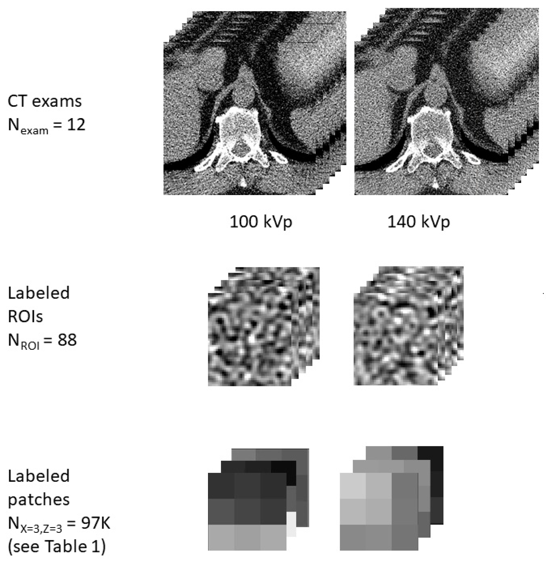
These 4-class labeled ROIs were input into an automated patch extraction process to generate thousands of non-overlapping 3D rectangular patches, each of size X by X by Z, where X and Z are odd numbers ≥ 3 that can be user-specified. X represents the pixel dimension of the square patch on axial imaging, while Z represents the craniocaudal dimension, i.e., the number of consecutive slices included. The following combinations of (X, Z) were used: (3, 3), (3, 5), (3, 7), (5, 5), (5, 7), and (7, 7), each with its own dataset of patches. As each patch has 3 spatial dimensions plus a dimension for CT acquisition energy, each patch is thus represented by a rank 4 tensor containing 16-bit grayscale pixel values (which represent Hounsfield units + 1024). Each tensor, therefore, encodes local information to assist in characterizing the center voxel and is associated with a tissue class label derived from its source ROI. CT data in the form of exams, ROIs, and patches are illustrated in Figure 2.

Figure 2.
Illustrative representation of examples of data used in this study in the form of CT exams, ROIs, and patches. The study includes data aggregated from 12 CT exams, 88 ROIs of various tissue classes, and thousands of patches of varying sizes, with a representative patch shown for a patch size of X = 3, Z = 3.
2.3. Machine Learning
The dataset consisted of tensors representing patches of dual-energy CT data, each paired with tissue class labels encoded as one-hot-encoding variables. The training, validation, and test sets were obtained from this dataset by random stratified selection using tissue class labels as the stratifying variable. In total, 20% of the dataset was used for individual model testing. Of the remaining data elements, 30% were used as validation, and 70% were used for training. Given the relative scarcity of intraspinal voxels and the primary goal of the study was to differentiate between the spinal cord and CSF, data augmentation was performed on the training and validation sets to increase the composition of intraspinal voxels. The set of tensors derived from intraspinal ROIs was augmented using flipping operations on each of the 3 spatial axes and rotation operations (90, 180, or 270 degrees) in the axial plane.
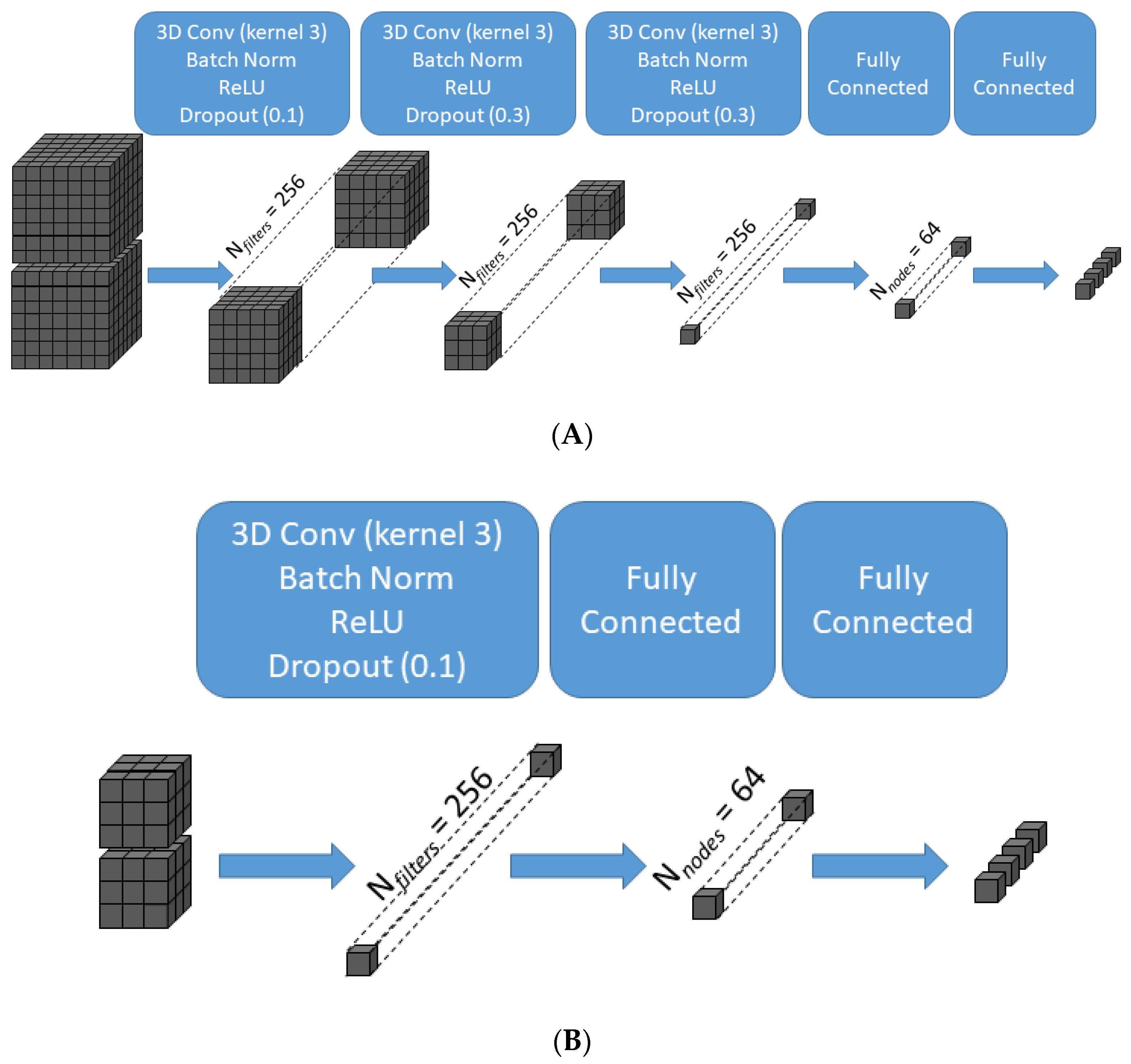
Supervised machine learning was implemented using the Sequential model in Keras, a deep learning application programming interface, to train a 4-class classifier neural network. The layer immediately below the input layer was a 3D convolutional layer with 256 filters and a 3 × 3 × 3 kernel without padding. Because padding was not used in the convolutions, the output of each convolutional layer is a 256-element array of data elements that are smaller than the data elements in its input. The number of layers in the network was allowed to vary with X or Z, such that higher values of X or Z would result in more convolution layers as needed to yield a 256-element array of scalar values prior to the fully connected layers (Figure 3). As our maximum patch size was 7 × 7 × 7 × 2, a maximum of 3 convolution layers were used. A batch-normalization step, a rectified linear unit (ReLU) activation function, and dropout were performed following each convolution. The most superficial convolutional layer had a dropout rate of 0.1, with higher dropout rates used at deeper layers. The penultimate layer was a dense layer with 64 nodes and a ReLU activation function. The final layer was a dense layer with a softmax activation function and a node for each of the four prediction classes.

Figure 3.
Schematic illustration of the transformation of data across the layers of the convolutional neural network for two representative patch sizes. For the largest patch size (X = 7, Z = 7) (A), the 7 × 7 × 7 × 2 input is transformed after three successive 3D convolutions of kernel size 3 × 3 × 3 without padding into a 256-element array of scalar values prior to the fully connected layers, which in turn generate the final 4-class classifier output. For the smallest patch size (X = 3, Z = 3) (B), one 3D convolution of kernel size 3 × 3 × 3 without padding is sufficient to generate a 256-element array of scalar values. 3D Conv = three-dimensional convolutional layer; Batch Norm = batch normalization layer; ReLU = rectified linear unit activation function.
Different models were independently trained and evaluated for each combination of X and Z. During training, models were fitted using the AdaDelta [21] optimizer with an initial learning rate of 0.001 and used categorical cross-entropy as the loss function. As described in [21], the AdaDelta optimizer is a variant of the stochastic gradient descent optimizer and was selected for its use of an adaptive learning rate throughout training. The training was performed for a maximum of 300K epochs, with early stopping if no improvement in validation loss was observed for 30K epochs. Performance metrics were obtained when applying individual models to the test set, and sensitivity/recall, specificity, precision/positive predictive value, and F1 scores for each tissue class were obtained. A final ensemble model was created by implementing an ensemble voting mechanism among 6 trained models such that the mode of the predicted class among these models determines the final class prediction. To assess transferability, performance metrics of the final model were evaluated on data generated from labeled ROIs in the holdout CT exam that was not used for training/validation.
2.4. Output Visualization
The final ensemble model was applied to selected CT lumbar spine exams to permit a visual assessment of the model’s ability to differentiate intraspinal CSF from spinal cord tissue. In addition to representative CT images among the 11 CTs used for training, this was also applied to the holdout CT exam to allow assessment of transferability to imaging volumes on which the network was not trained or validated. For each voxel in a CT exam (except for voxels located within 3 pixels of the edge), a tensor was generated to capture pixel intensities of the 7 × 7 × 7 group of voxels centered at the voxel of interest at low and high energies. This tensor was then sent as input to the final ensemble model to predict the center voxel tissue class. To assist with the visualization of intraspinal anatomy, output image maps were generated in 8-bit grayscale to depict voxel assignments to each of the 4 tissue classes. Voxels classified as bone were assigned a low pixel value of 1 to effect bone subtraction. Fat voxels were assigned slightly higher pixel values (50), water voxels were assigned a high pixel value of 200 to simulate myelography, and soft tissue voxels were assigned a fixed intermediate value of 100.
3. Results
3.1. Model Training
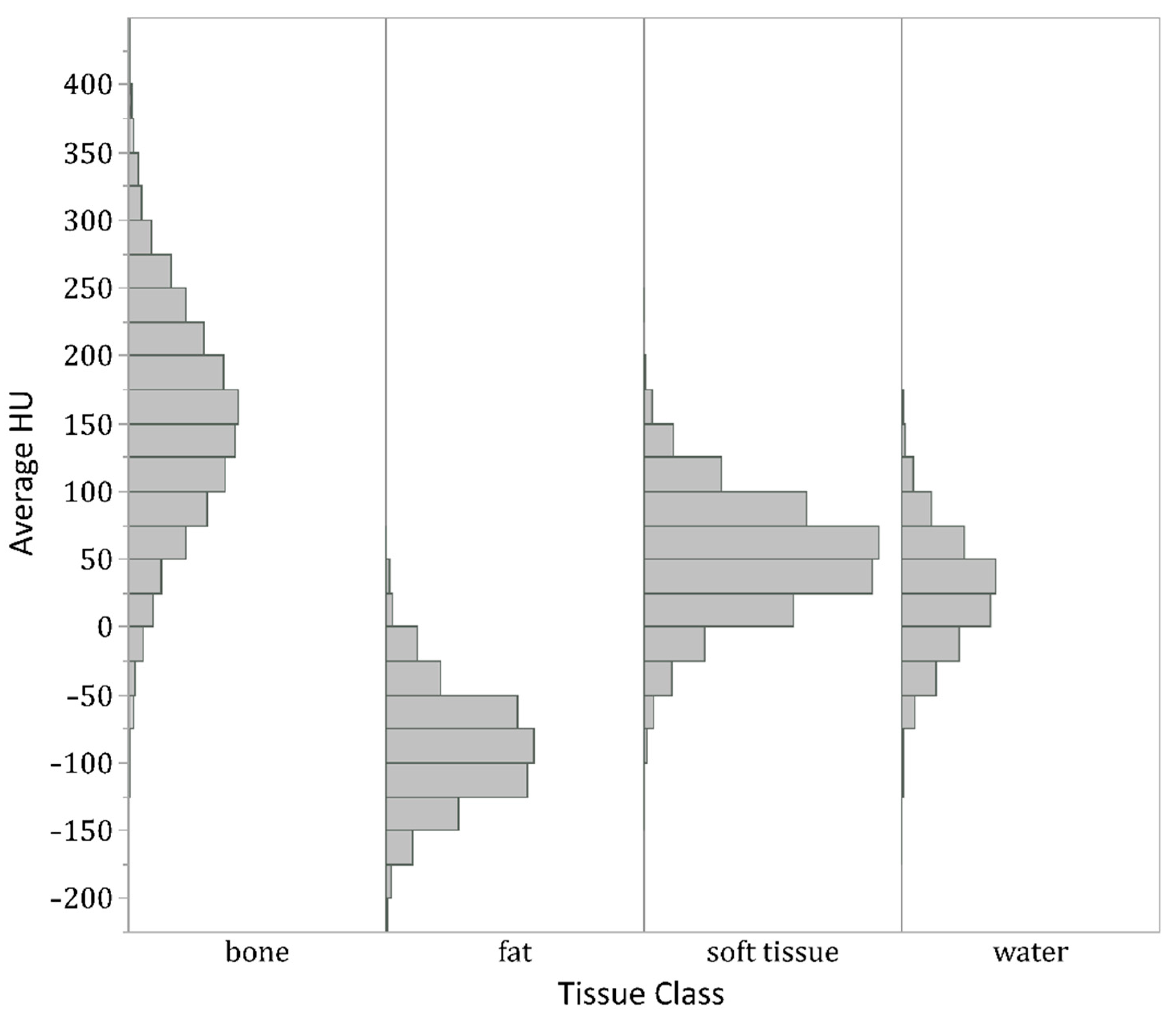
At each patch size, machine learning models were trained to identify the tissue class of the center voxel. The number of patches in the datasets used in training and individual model testing/validation varied with patch size (Table 1), such that smaller sizes allowed for the generation of more patches from the labeled ROIs, ranging from >97,000 for the smallest size of 3 × 3 × 3 × 2 to approximately 6500 for 7 × 7 × 7 × 2. There was class imbalance, with relative underrepresentation of the ‘water’ class related to difficulty obtaining large ROIs for this class. The overlap in center-pixel Hounsfield units (HU) across tissue classes for the largest of the labeled datasets (Figure 4) confirms the difficulty of HU-based thresholding methods in differentiating these tissue types.

Table 1.
Composition of the labeled dataset used for training and individual model testing. Entries in each cell represent numbers of non-overlapping X by X by Z by 2 tensors in the labeled dataset.
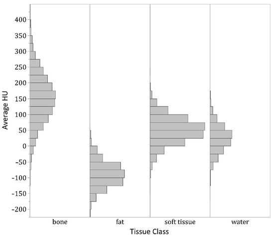
Figure 4.
Histogram of average center Hounsfield units (HU) of all 3 × 3 × 3 × 2 patches generated from the labeled ROIs. Although center pixels in patches from bone ROIs, not unexpectedly, show higher HUs on average than water and soft tissue patches, and fat patches show lower HUs, the tissue classes show substantial overlap in HUs. In particular, the histograms for soft tissue and water are nearly superimposable. Therefore, no HU thresholding could separate all four classes with high accuracy.
These patches were used to train convolutional neural networks, and representative learning curves are shown in Figure 5. At the smallest patch size evaluated (3 × 3 × 3 × 2), the loss or accuracy curves for training and validation are nearly superimposed. Some overfitting is observed at larger patch sizes, but overall validation accuracy remained high. A patch size of 3 × 3 × 3 × 2 provided the greatest overall test accuracy of 99.8%, with larger sizes resulting in slightly lower test accuracies ranging from 98.1% to 99.0% (Table 2). Among the four tissue classes, the ‘water’ class was associated with the worst performance at some of the higher patch sizes, possibly related to relative underrepresentation of this class (Table 2), but overall test accuracy for this class and the remaining classes exceeded 98% for all values of X and Z examined. F1 scores, which may be more useful in the setting of class imbalance, ranged from 94.2% to 99.3% for the ‘water’ class and consistently exceeded 98% for the other three classes (Table 2).

Figure 5.
Representative learning curves. For the smallest patch size of 3 × 3 × 3 × 2 (A), the training and validation curves are nearly superimposed when assessing either accuracy or loss. At a patch size of 7 × 7 × 7 × 2 (B), optimal training accuracy and loss are slightly better than for validation.
Table 2.
Confusion matrices and detailed test performance characteristics a at different combinations of X and Z.
These six models were combined into an ensemble model for subsequent application to dual-energy CT volumes. The ensemble model performed satisfactorily on the holdout CT exam, with an accuracy of 99.4% (Table 3). Sensitivities ranged from 100.0% for bone and fat to 90.0% for water, and specificities ranged from 99.6% for bone and water to 100% for soft tissue and fat (Table 3). Note that these metrics represent performance on homogenous ROIs of each tissue class, which were much smaller than the source CT volumes, and the assessment of the model performance on voxels outside these selected ROIs requires visualization of the generated post-processed images in the subsequent section.
Table 3.
Confusion matrix and detailed test performance characteristics a of the final ensemble model.
3.2. Visualization of Post-Processed Images
We assessed four-class classifier performance in areas beyond the selected ROIs by using the ensemble model to generate output images at four distinct grayscale values to represent water, soft tissue, fat, and bone (in order of decreasing pixel values). The generated images allow for the depiction of the conus medullaris and cauda equina among a background of high CSF pixel intensity, thereby simulating a post-myelogram CT image with bone subtraction (Figure 6). Because the model was trained only on homogenous patches, suboptimal tissue discrimination at tissue interfaces is not unexpected. Image quality on the holdout test CT (Figure 6B) is comparable to that on a representative CT exam among the 11 used for training (Figure 6A).
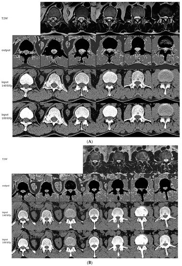
Figure 6.
Representative images generated by the ensemble model as applied to 1 of the 11 CT exams used for individual model training/validation (A) and to the holdout CT exam that was not used for training (B). The montages show generated 4-scale output images (2nd row), original 0.75 mm CT images at 140 kVp (3rd row), and original 0.75 mm CT images at 100 kVp (4th row). Each column of CT images shown represents slices at 2.25 cm intervals. Corresponding 5 mm axial T2W MRI images are shown in the 1st row for comparison.
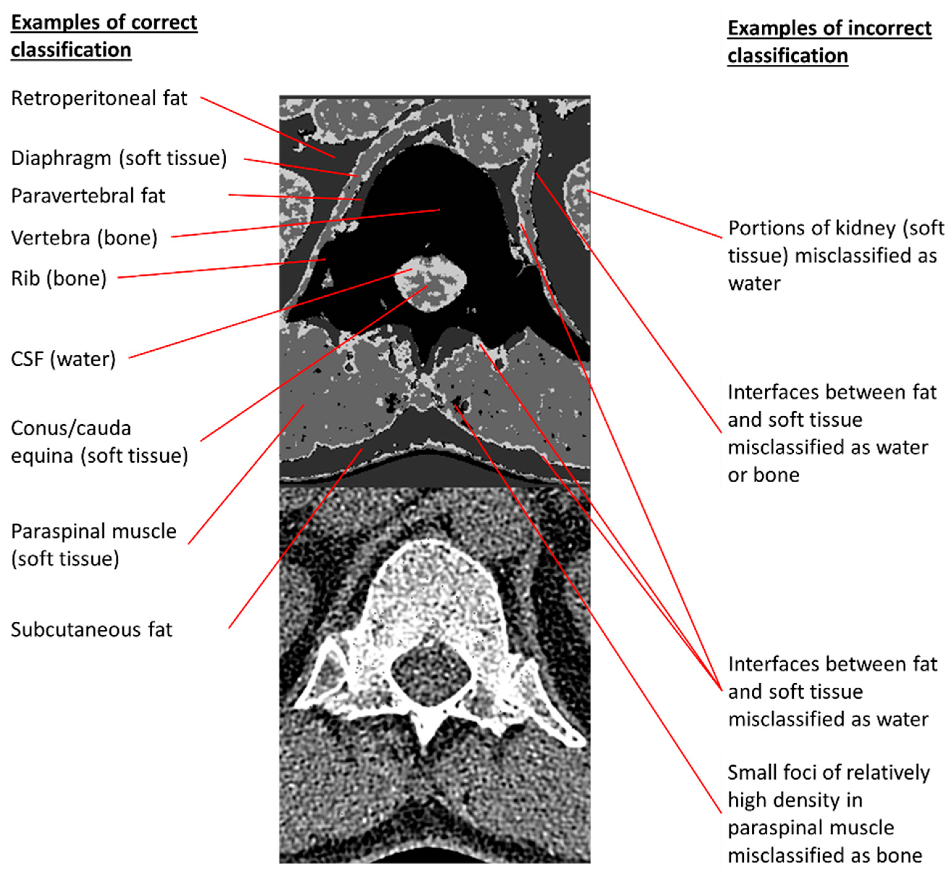
The qualitative inspection of the generated images and the comparison to MRI reveals some discrepancies between the MRI reference standard and the model’s depiction of CSF and neural tissue. For instance, in Figure 6A, the area occupied by CSF in each axial image is mildly overestimated, and the model is not able to depict individual cauda equina nerve roots at lower levels, presumably due to their small size on cross-sectional imaging. In Figure 6B, some of the nerve roots are better depicted, and canal stenosis (seen as a loss of the T2-weighted signal in the thecal sac in the penultimate column) can be visualized on the generated four-scale images. Figure 7 further illustrates examples of correct and incorrect tissue classification in a magnified view of a selected output image near the thoracolumbar junction. For this purpose, the correctness of tissue classification was based on the comparison to its expected appearance on CT or MRI. Note that the source and output images include several structures not included in any of the labeled training or testing ROIs. For instance, paravertebral fat, diaphragm, and ribs generally produce correct pixel classification despite the lack of inclusion of these structures in any of the labeled ROIs. Kidneys and tissue interfaces (which contain more than one tissue class) were not included in the labeled ROIs and contribute to common instances of misclassification.
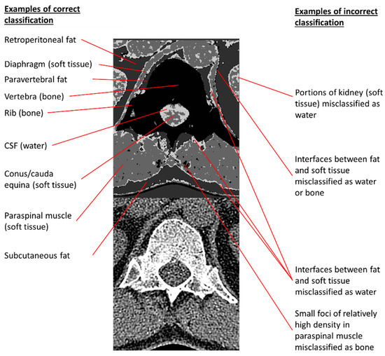
Figure 7.
Examples of correct and incorrect tissue classifications in a representative output image taken from the second column of Figure 6A. The 140 kVp CT source image is placed below the annotated output image to permit comparisons of annotated pixels to their corresponding CT appearances.
4. Discussion
In this study, we developed a novel machine learning model to assist the visualization of intraspinal soft tissue structures on an unenhanced dual-energy spine CT by differentiating four major tissue classes with high accuracy. We trained and tested multiple convolutional neural networks to perform the task of classifying a small 3D patch of a CT volume using HUs at both 100 kVp and 140 kVp in the center voxel and surrounding voxels. We found that an ensemble model, consisting of six individually trained models that differ in the number of surrounding voxels they accept as input, showed 99.4% overall accuracy on labeled ROIs from a holdout test CT exam not used for training/validation. The accuracy is much higher than would be expected for this task when relying on visual assessment, especially since HUs alone cannot reliably separate water pixels from soft tissue, given their near-identical HU distributions, as shown in Figure 4. Among the tissue types, fat and bone show the best classification. Sensitivity and specificity for fat classification were both 100.0% in the holdout test set. Our bone voxel prediction, with 100% sensitivity and 99.6% specificity in our holdout test set, is mildly more accurate than prior studies using machine learning to segment bone from adjacent soft tissues (91–97% sensitivity and 93–99% specificity [13,14]). For the more difficult task of identifying soft tissue and water voxels, which to our knowledge has not been performed in this setting, the ensemble model performs relatively well, with test sensitivities of 98.6% and 90.0% and specificities of 100.0% and 99.6% for the soft tissue and water classes, respectively.
Although the mechanisms by which the model performs this discrimination task are not readily explainable, one interpretation is that low-level features, such as combinations of Hounsfield units, texture, and differences in low-energy and high-energy HUs, are sufficiently different among the four tissue types to allow the model to successfully identify the appropriate tissue class. Since the model performs the task using only small 3D volumes as input, no voxels more than three units from the center voxel in any dimension are available to the model during the classification task. Therefore, an advantage of this patch-based approach to segmentation compared to using the entire CT volume as input to a deep learning segmentation model is that the model does not rely on spatial information provided by macroscopic elements, such as the relationship to bony structures or anatomical location, to deduce a voxel’s membership in a given class. While such information could potentially improve performance, the reliance on high-level features and global spatial cues would likely introduce undesired biases (e.g., predicting water class for voxels based on their location in the lower lumbar spine) that may compromise performance in case of abnormal pathology. Another advantage is that a large number of training elements was able to be generated from a small number of CT exams, which is useful for exams like dual-energy spine CT that are not routinely requested in clinical practice. Since only homogenous single-class patches are provided to the model for training, one disadvantage of this approach is that the model performs poorly at interfaces between two or more tissue types.
Among the major implications of our study is that machine learning can distinguish between intraspinal neural tissue and CSF much better than is considered possible for radiologists reviewing the source dual-energy CT images (Figure 4). The relatively high overlap in attenuation levels between soft tissue and water pixels (Figure 2) precludes any conventional thresholding or window-leveling approach from separating these pixels on the original CT source images. The neural network, therefore, was charged with a much more difficult task than simply replicating what a radiologist sees; it instead performed satisfactorily in discerning subtle tissue differences imperceptible to radiologists. From a clinical perspective, our neural network model has the potential to improve the visualization of intraspinal soft tissue and may lead to better post-processing methods to assist radiologists’ interpretation of dual-energy spine CT.
To our knowledge, this patch-based machine learning strategy to segment a dual-energy CT to better visualize intraspinal CSF has not been previously described. Patch-based features have recently been used in other deep learning architectures for such tasks as brain MRI segmentation [22]. Other deep learning techniques, such as generative adversarial networks, have been used to synthetically improve the visualization of brain MRI findings by simulating full-dose contrast enhancement in patients receiving no or reduced amounts of gadolinium [23,24]. In these scenarios, machine learning was applied to capture subtle relationships and patterns that predict the appearance on a more sensitive imaging technique. In our study, we created synthetic images to augment visualization of CSF on unenhanced dual-energy spine CT images, akin to a “virtual myelogram.” Our findings may lead to automated techniques that could be evaluated in subsequent studies to improve the diagnosis or detection of severe spinal stenosis or other intraspinal abnormalities. However, future clinical studies would be needed to validate the use of this or similar methods in detecting intraspinal pathology, such as cord compression, large disc herniations, or epidural tumor, before such approaches could be adopted in clinical practice.
Among the limitations of this study is that our models were trained and tested in a small number of spine CTs, all from the same scanner model and manufacturer at a single institution, thus potentially benefiting from the similarity of scan parameters. The transferability to other scan conditions was not tested in this study, and future work may need to include a greater variety of scanner types and more exam types to ensure model robustness. The generated segmentation images also illustrate some shortcomings of model performance, such as the false-positive depiction of water voxels outside the spine. This may be due in part to the decision to selectively augment intraspinal voxels to improve performance in intraspinal tissue differentiation, which is likely justified given the emphasis on intraspinal anatomy in this study. Third, the model was developed using only exams with relatively normal intraspinal anatomy; therefore, its performance in a clinical setting to facilitate diagnosis or detection of intraspinal pathology has not been tested.
5. Conclusions
In this study, we demonstrated that an ensemble of CNNs taking small 3D patches of dual-energy CT data as input can satisfactorily perform a four-tissue voxel classification task with high accuracy (99.4% four-class test classification accuracy). The performance was best for fat and bone voxels but also satisfactory for our main objective of classifying soft tissue and water voxels, with test sensitivity and specificity for soft tissue and test specificity for water approaching 99–100%, and a test sensitivity for water of 90%. This model was used to produce segmented output images permitting the qualitative assessment of intra-spinal fluid volume, which could be of potential use in assisting the detection of pathological spine conditions, such as spinal stenosis. While limitations of the study include the small number of CT exams used, a lack of diversity of intraspinal pathology and scanner models or manufacturers, and the presence of some false classifications (particularly in locations such as fat–soft tissue interfaces that are not included in the training set), the current study establishes a proof of concept that local low-level features on dual-energy spine CT contain sufficient information to permit accurate pixel classification and enhance the visualization of intraspinal neural tissue, although not quite as well as MRI. Future work on this topic would include further characterization and refinement of the model, such as training and testing on a wider variety of scanner manufacturers and models, different acquisition settings, a higher number of patients, and a wider variety of intraspinal pathology.
Author Contributions
Conceptualization, X.V.N.; methodology, X.V.N., E.D., S.C. and L.M.P.; software, X.V.N., D.D.N. and E.D.; validation, X.V.N., D.D.N., E.D., S.C. and L.M.P.; formal analysis, X.V.N. and D.D.N.; investigation, X.V.N., D.D.N., E.D., S.C. and L.M.P.; resources, L.M.P.; data curation, X.V.N. and D.J.B.; writing—original draft preparation, X.V.N.; writing—review and editing, X.V.N., D.D.N., E.D., S.C., D.J.B. and L.M.P.; visualization, X.V.N. and D.D.N.; supervision, X.V.N. and L.M.P.; project administration, X.V.N. and L.M.P.; funding acquisition, X.V.N. and L.M.P. All authors have read and agreed to the published version of the manuscript.
Funding
This research received no external funding.
Institutional Review Board Statement
The study was conducted in accordance with the Declaration of Helsinki and approved by the Biomedical Sciences Institutional Review Board of the Ohio State University, along with waivers of HIPAA authorization and informed consent (protocol # 2019H0094; date of approval: 18 March 2019).
Informed Consent Statement
Patient consent was waived by the IRB due to involvement of no more than minimal risk given the retrospective design of the study.
Data Availability Statement
The data presented in this study are available on request from the corresponding author. The data are not publicly available due to patient data not being authorized for public dissemination.
Conflicts of Interest
X.V.N. reports stock ownership and/or dividends from the following companies broadly relevant to AI services or hardware: Alphabet, Amazon, Apple, AMD, Microsoft, and NVIDIA. E.D. and L.M.P have patents relevant to AI in medical imaging but they are unrelated to the topic of this manuscript. The authors declare that they have no other conflict of interest.
References
- Tins, B.J. Imaging investigations in Spine Trauma: The value of commonly used imaging modalities and emerging imaging modalities. J. Clin. Orthop. Trauma 2017, 8, 107–115. [Google Scholar] [CrossRef]
- Nkusi, A.E.; Muneza, S.; Hakizimana, D.; Nshuti, S.; Munyemana, P. Missed or Delayed Cervical Spine or Spinal Cord Injuries Treated at a Tertiary Referral Hospital in Rwanda. World Neurosurg. 2016, 87, 269–276. [Google Scholar] [CrossRef] [PubMed]
- Andre, J.B.; Bresnahan, B.W.; Mossa-Basha, M.; Hoff, M.N.; Smith, C.P.; Anzai, Y.; Cohen, W.A. Toward Quantifying the Prevalence, Severity, and Cost Associated with Patient Motion During Clinical MR Examinations. J. Am. Coll. Radiol. 2015, 12, 689–695. [Google Scholar] [CrossRef] [PubMed]
- Nguyen, X.V.; Tahir, S.; Bresnahan, B.W.; Andre, J.B.; Lang, E.V.; Mossa-Basha, M.; Mayr, N.A.; Bourekas, E.C. Prevalence and Financial Impact of Claustrophobia, Anxiety, Patient Motion, and Other Patient Events in Magnetic Resonance Imaging. Top. Magn. Reson. Imaging 2020, 29, 125–130. [Google Scholar] [CrossRef] [PubMed]
- Pomerantz, S.R. Myelography: Modern technique and indications. Handb. Clin. Neurol. 2016, 135, 193–208. [Google Scholar] [CrossRef] [PubMed]
- Patino, M.; Prochowski, A.; Agrawal, M.D.; Simeone, F.J.; Gupta, R.; Hahn, P.F.; Sahani, D.V. Material Separation Using Dual-Energy CT: Current and Emerging Applications. Radiographics 2016, 36, 1087–1105. [Google Scholar] [CrossRef]
- Mallinson, P.I.; Coupal, T.M.; McLaughlin, P.D.; Nicolaou, S.; Munk, P.L.; Ouellette, H.A. Dual-Energy CT for the Musculoskeletal System. Radiology 2016, 281, 690–707. [Google Scholar] [CrossRef]
- Yun, S.Y.; Heo, Y.J.; Jeong, H.W.; Baek, J.W.; Choo, H.J.; Shin, G.W.; Kim, S.T.; Jeong, Y.G.; Lee, J.Y.; Jung, H.S. Dual-energy CT angiography-derived virtual non-contrast images for follow-up of patients with surgically clipped aneurysms: A retrospective study. Neuroradiology 2019, 61, 747–755. [Google Scholar] [CrossRef]
- Long, Z.; DeLone, D.R.; Kotsenas, A.L.; Lehman, V.T.; Nagelschneider, A.A.; Michalak, G.J.; Fletcher, J.G.; McCollough, C.H.; Yu, L. Clinical Assessment of Metal Artifact Reduction Methods in Dual-Energy CT Examinations of Instrumented Spines. AJR Am. J. Roentgenol. 2019, 212, 395–401. [Google Scholar] [CrossRef]
- Nguyen, X.V.; Oztek, M.A.; Nelakurti, D.D.; Brunnquell, C.L.; Mossa-Basha, M.; Haynor, D.R.; Prevedello, L.M. Applying Artificial Intelligence to Mitigate Effects of Patient Motion or Other Complicating Factors on Image Quality. Top. Magn. Reson. Imaging 2020, 29, 175–180. [Google Scholar] [CrossRef]
- Richardson, M.L.; Garwood, E.R.; Lee, Y.; Li, M.D.; Lo, H.S.; Nagaraju, A.; Nguyen, X.V.; Probyn, L.; Rajiah, P.; Sin, J.; et al. Noninterpretive Uses of Artificial Intelligence in Radiology. Acad. Radiol. 2020, 28, 1225–1235. [Google Scholar] [CrossRef] [PubMed]
- Lakhani, P.; Prater, A.B.; Hutson, R.K.; Andriole, K.P.; Dreyer, K.J.; Morey, J.; Prevedello, L.M.; Clark, T.J.; Geis, J.R.; Itri, J.N.; et al. Machine Learning in Radiology: Applications Beyond Image Interpretation. J. Am. Coll. Radiol. 2018, 15, 350–359. [Google Scholar] [CrossRef] [PubMed]
- Vania, M.; Mureja, D.; Lee, D. Automatic spine segmentation from CT images using Convolutional Neural Network via redundant generation of class labels. J. Comput. Des. Eng. 2019, 6, 224–232. [Google Scholar] [CrossRef]
- Qadri, S.F.; Ai, D.; Hu, G.; Ahmad, M.; Huang, Y.; Wang, Y.; Yang, J. Automatic Deep Feature Learning via Patch-Based Deep Belief Network for Vertebrae Segmentation in CT Images. Appl. Sci. 2018, 9, 69. [Google Scholar] [CrossRef]
- Khandelwal, P.; Collins, D.L.; Siddiqi, K. Spine and Individual Vertebrae Segmentation in Computed Tomography Images Using Geometric Flows and Shape Priors. Front. Comput. Sci. 2021, 3, 66. [Google Scholar] [CrossRef]
- Fan, G.; Liu, H.; Wu, Z.; Li, Y.; Feng, C.; Wang, D.; Luo, J.; Wells, W.M.; He, S. Deep Learning-Based Automatic Segmentation of Lumbosacral Nerves on CT for Spinal Intervention: A Translational Study. AJNR Am. J. Neuroradiol. 2019, 40, 1074–1081. [Google Scholar] [CrossRef]
- Diniz, J.O.B.; Diniz, P.H.B.; Valente, T.L.A.; Silva, A.C.; Paiva, A.C. Spinal cord detection in planning CT for radiotherapy through adaptive template matching, IMSLIC and convolutional neural networks. Comput. Methods Programs Biomed. 2019, 170, 53–67. [Google Scholar] [CrossRef]
- Kraus, M.; Weiss, J.; Selo, N.; Flohr, T.; Notohamiprodjo, M.; Bamberg, F.; Nikolaou, K.; Othman, A.E. Spinal dual-energy computed tomography: Improved visualisation of spinal tumorous growth with a noise-optimised advanced monoenergetic post-processing algorithm. Neuroradiology 2016, 58, 1093–1102. [Google Scholar] [CrossRef]
- Schindelin, J.; Arganda-Carreras, I.; Frise, E.; Kaynig, V.; Longair, M.; Pietzsch, T.; Preibisch, S.; Rueden, C.; Saalfeld, S.; Schmid, B.; et al. Fiji: An open-source platform for biological-image analysis. Nat. Methods 2012, 9, 676–682. [Google Scholar] [CrossRef]
- Xie, S.; Yang, T.; Wang, X.; Lin, Y. Hyper-class augmented and regularized deep learning for fine-grained image classification. In Proceedings of the IEEE Conference on Computer Vision and Pattern Recognition, Boston, MA, USA, 7–12 June 2015; pp. 2645–2654. [Google Scholar] [CrossRef]
- Zeiler, M.D. ADADELTA: An Adaptive Learning Rate Method. arXiv 2012, arXiv:1212.5701. [Google Scholar]
- Lee, B.; Yamanakkanavar, N.; Choi, J.Y. Automatic segmentation of brain MRI using a novel patch-wise U-net deep architecture. PLoS ONE 2020, 15, e0236493. [Google Scholar] [CrossRef] [PubMed]
- Gong, E.; Pauly, J.M.; Wintermark, M.; Zaharchuk, G. Deep learning enables reduced gadolinium dose for contrast-enhanced brain MRI. J. Magn. Reson. Imaging 2018, 48, 330–340. [Google Scholar] [CrossRef] [PubMed]
- Kleesiek, J.; Morshuis, J.N.; Isensee, F.; Deike-Hofmann, K.; Paech, D.; Kickingereder, P.; Kothe, U.; Rother, C.; Forsting, M.; Wick, W.; et al. Can Virtual Contrast Enhancement in Brain MRI Replace Gadolinium?: A Feasibility Study. Investig. Radiol. 2019, 54, 653–660. [Google Scholar] [CrossRef] [PubMed]


Publisher’s Note: MDPI stays neutral with regard to jurisdictional claims in published maps and institutional affiliations. |
© 2022 by the authors. Licensee MDPI, Basel, Switzerland. This article is an open access article distributed under the terms and conditions of the Creative Commons Attribution (CC BY) license (https://creativecommons.org/licenses/by/4.0/).