Abstract
Approximate adders are some of the fundamental arithmetic operators that are being employed in error-resilient applications, to achieve performance/energy/area gains. This improvement usually comes at the cost of some accuracy and, therefore, requires prior error analysis, to select an approximate adder variant that provides acceptable accuracy. Most of the state-of-the-art error analysis techniques for approximate adders assume input bits and operands to be independent of one another, while some also assume the operands to be uniformly distributed. In this paper, we analyze the impact of these assumptions on the accuracy of error estimation techniques, and we highlight the need to address these assumptions, to achieve better and more realistic quality estimates. Based on our analysis, we propose DAEM, a data- and application-aware error analysis methodology for approximate adders. Unlike existing error analysis models, we neither assume the adder operands to be uniformly distributed nor assume them to be independent. Specifically, we use 2D joint input probability mass functions (PMFs), populated using sample data, in order to incorporate the data and application knowledge in the analysis. These 2D joint input PMFs, along with 2D error maps of approximate adders, are used to estimate the error PMF of an adder network. The error PMF is then utilized to compute different error measures, such as the mean squared error (MSE) and mean error distance (MED). We evaluate the proposed error analysis methodology on audio and video processing applications, and we demonstrate that our methodology provides error estimates having a better correlation with the simulation results, as compared to the state-of-the-art techniques.
1. Introduction
Approximate computing can be employed to gain benefits in terms of performance, energy and/or area, by relaxing the bounds of precise computing [1,2,3,4,5]. Recent investigations suggest that there are a number of computationally intensive applications that can tolerate approximation errors while still producing outputs that are of acceptable quality for the end-users [6,7,8,9,10]. Specifically, applications such as image/video processing, multimedia, machine learning, big data analytics and recognition are intrinsically prone to noise and/or are resilient to error because of the perceptual limitations of the end-users and, hence, are suitable candidates for approximate computing [2,4,11].
Recently, an emerging trend has been observed towards using reconfigurable architectures, like coarse-grained reconfigurable architectures (CGRAs) [12,13,14,15,16], as accelerators, along with general-purpose processors, to improve the energy and performance efficiency of an application. These architectures allow us to implement data flow graphs (DFGs) without much effort, by merely configuring the processing elements (PEs) and the connections between them. Several works have been carried out to improve the performance and energy efficiency of CGRAs, by deploying approximations in the arithmetic components inside the PEs [16]. However, to maintain the usability of the same hardware for different applications that can react to approximations differently, the approximate components are designed to be accuracy-configurable, e.g., the gracefully degrading accuracy-configurable adder (GDA) [17], which is an accuracy-configurable low-latency approximate adder.
Several applications that fall under the umbrella of error-tolerant applications—e.g., filtering, image processing and machine learning—make use of cascaded adder modules or adder trees [18]. These applications can significantly benefit from hardware, like approximate CGRAs. However, selecting a suitable configuration, which meets the user-defined accuracy constraint while maximizing the desired efficiency metric, requires a sophisticated error estimation method that can estimate the error of all the configurations supported by the hardware. Such an error estimation method is also required at design time to select the appropriate type of configurable module (i.e., in this case, an accuracy-configurable adder) with the most suitable set of configurations. Below, we provide an overview of the state-of-the-art schemes/techniques that provide error estimation for such approximate arithmetic modules.
1.1. State-of-the-Art and Their Key Limitations
Various techniques have been proposed in the literature for the error estimation of approximate adders [19,20,21,22,23,24,25,26,27]. In [19], Liu et al. proposed a framework for the error analysis of approximate adders used specifically for the accumulation of partial products in an approximate multiplier. The algorithm uses a single full adder as the basic element, and it employs data-specific knowledge to populate the probability distribution for each bit location. However, there are two major shortcomings of this approach. First, the proposed bit-wise distribution considers each bit to be independent. Secondly, it assumes the two adder operands to be independent of each other. Along similar lines, PEAL [20] and PEMACx [21] presented techniques to estimate the error metrics of low-power approximate adders composed of cascaded approximate units. However, the techniques were based on the same two assumptions. We show later, in the motivational analysis (in Section 3), that these two assumptions are not always valid for real applications. In [22], the authors presented analytical error models for approximate adders while assuming a uniform distribution for the inputs. The work mainly estimated the error characteristics of only three types of adders, i.e., the error segmentation adder (ESA), the almost-correct Adder (ACA) and the error-tolerant adder type II (ETA-II). However, it did not provide a generalized model that could be extended to other low-latency adder structures, such as GDA and GeAr. To address this limitation, Mazahir et al. [23] presented a generalized analytical model for error estimation, which is applicable to a wide range of low-latency approximate adders that comprise sub-adder units of uniform as well as non-uniform lengths. The model allows the use of any arbitrary data distribution to specify the inputs of a two-operand addition. This allows the application designer to populate the distribution by using sample data and, thus, to incorporate application and data knowledge into the error analysis. However, the two operands of an adder are still assumed to be independent. Furthermore, for multi-operand addition, the inputs belonging to different adders are also assumed to be independent.
Apart from the abovementioned works, recently, Dou et al. [24] presented a PMF-based error estimation technique. However, they assumed the PMFs of the error to be independent of the inputs, and they also assumed the nodes to be independent of one another. The technique improved the work proposed in [25], which also assumed the nodes to be independent of one another. Another work aimed at quantifying the error metrics of approximate datapaths was [26], and it also assumed the input bits, operands and nodes to be independent of one another, to simplify the error estimation process.
In summary, all the previously mentioned analytical methods either assume the inputs to be independent [19,20,21,22,23,25,26] and/or assume the input data to be uniformly distributed [22,27]. Hence, they are unable to take into account the complete data and application knowledge that is necessary for accurate error estimation, as also highlighted in the motivational case study (in Section 3).
1.2. Our Novel Contributions
In this paper, we analyze the impact of commonly employed assumptions in error estimation techniques for approximate adders on the accuracy of generated estimates, and we highlight the need to relax these assumptions to achieve reasonable results. Based on our findings, we present a novel data- and application-aware error analysis methodology (DAEM) that neither assumes the adder operands to be uniformly distributed nor assumes them to be independent. Its key features are discussed below.
- DAEM employs two-dimensional joint input PMFs, populated over application data. These PMFs not only incorporate the specific input data distribution of the two operands, but they also characterize the joint probability of the occurrence of each possible input combination of the adder operands.
- Using a probabilistic analysis approach, DAEM provides a technique for the estimation of the PMF of the error at the output of an approximate adder. The PMF further allows the computation of the two predominantly used error matrices, i.e., mean square error (MSE) and mean error distance (MED). Furthermore, our DAEM methodology is extendable to datapaths composed of multiple adders.
- DAEM is applicable to a wide range of low-latency approximate adder designs, such as GDA, GeAr, ESA, ETAII, ETAIIM, ACA and ACAA [28]. We demonstrate this in Section 5 by using the proposed methodology for different GeAr configurations, as the GeAr adder model can be configured to mimic the functional characteristics (mainly the input–output transformation model) of most of these adder designs.
We also provide experimental evidence suggesting that, by utilizing the proposed DAEM methodology, we can achieve a realistic error estimate for approximate adders. We show this for a number of representative tasks/applications from the multimedia domain.
2. Background
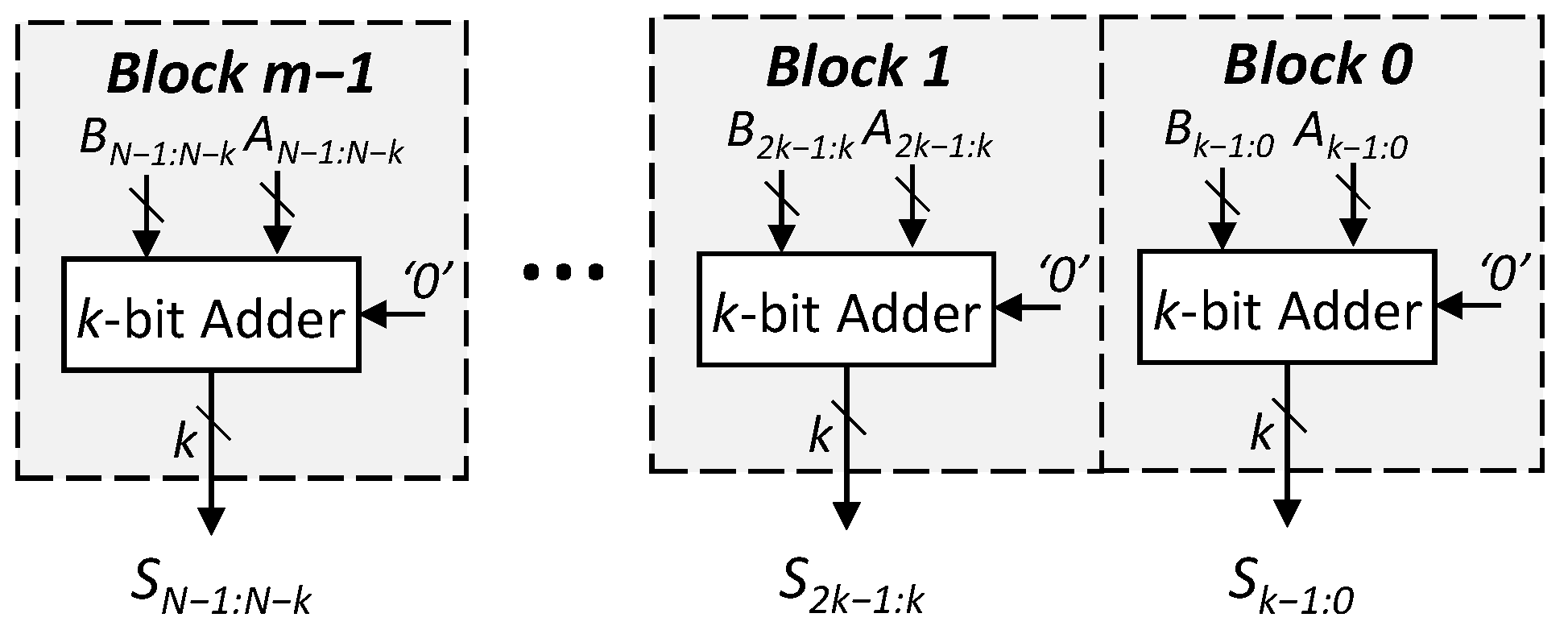
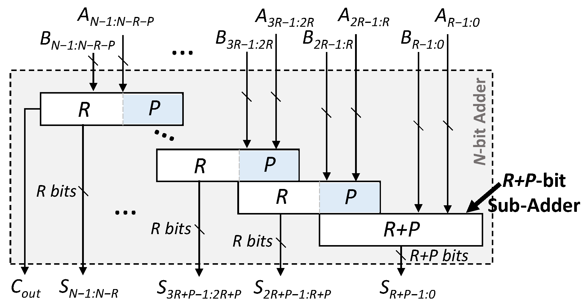
In the past few years, the design of low-latency approximate adders has received a significant amount of attention from the approximate computing community [17,29,30,31,32,33,34], to improve the performance, area and power efficiency of error-resilient applications. A dominant subset of these adders, which includes segmented and carry select adders (Figure 1 and Figure 2, respectively), is based on the idea that, for most of the input combinations, the longest carry propagation chain is less than the complete length (N) of the adder [28]. This allows designers to break the carry chain of an adder by using multiple smaller disjoint or overlapping sub-adders [29]. Each sub-adder makes use of P number of previous bits to predict the carry and produces R number of resultant bits, which directly contribute to the final sum bits. Some prominent examples of these high-performance adders [28] include the error-tolerant adders (ETAs) [11,31,35,36], the almost-correct adder (ACA-I) [29], the variable-latency speculative adder (VLSA) [29], the accuracy-configurable adder (ACA-II) [30], the gracefully degrading adder (GDA) [17] and the generic accuracy-configurable adder (GeAr) [32]. Figure 3 illustrates the GeAr adder structure, which can be used to represent almost all the low-latency approximate adder designs, as well as further design variants, by varying the number of resultant (R) and the number of prediction (P) bits. For example, the structure of the error-tolerant adder II (ETAII), shown in Figure 4, can be represented by defining P to be equal to R.
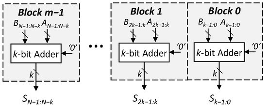
Figure 1.
Structure of the equally segmented adder. All the sub-adders compute the result independently from one another. The carry does not propagate from one block to the other and, therefore, the latency of the design is significantly lower than that of its accurate counterpart.
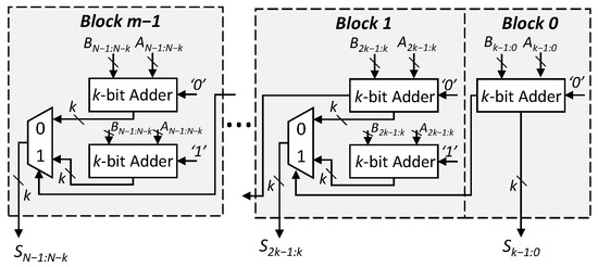
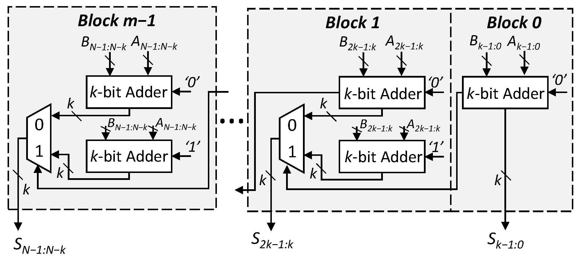
Figure 2.
Structure of the speculative carry select adder. The output of each block is based on the carry from the previous block.

Figure 3.
Structure of the generic accuracy-configurable adder (GeAr). In this model, a specific low-latency approximate adder configuration can be defined by defining the number of resultant (R) bits and the number of propagation (P) bits. R defines the number of sum bits generated by each sub-adder, excluding the least significant sub-adder, as it generates R + P sum bits. P, in general, defines the number of bits in each sub-adder that are overlapping with its previous sub-adder. Thus, the GeAr configurations are represented in text using the ‘GeAr(N,R,P)’ notation.
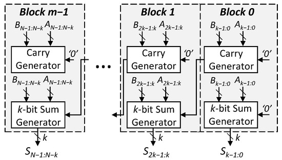
Figure 4.
Structure of the error-tolerant adder type II (ETAII). The carry generation unit in each block computes the carry for its corresponding subsequent block.
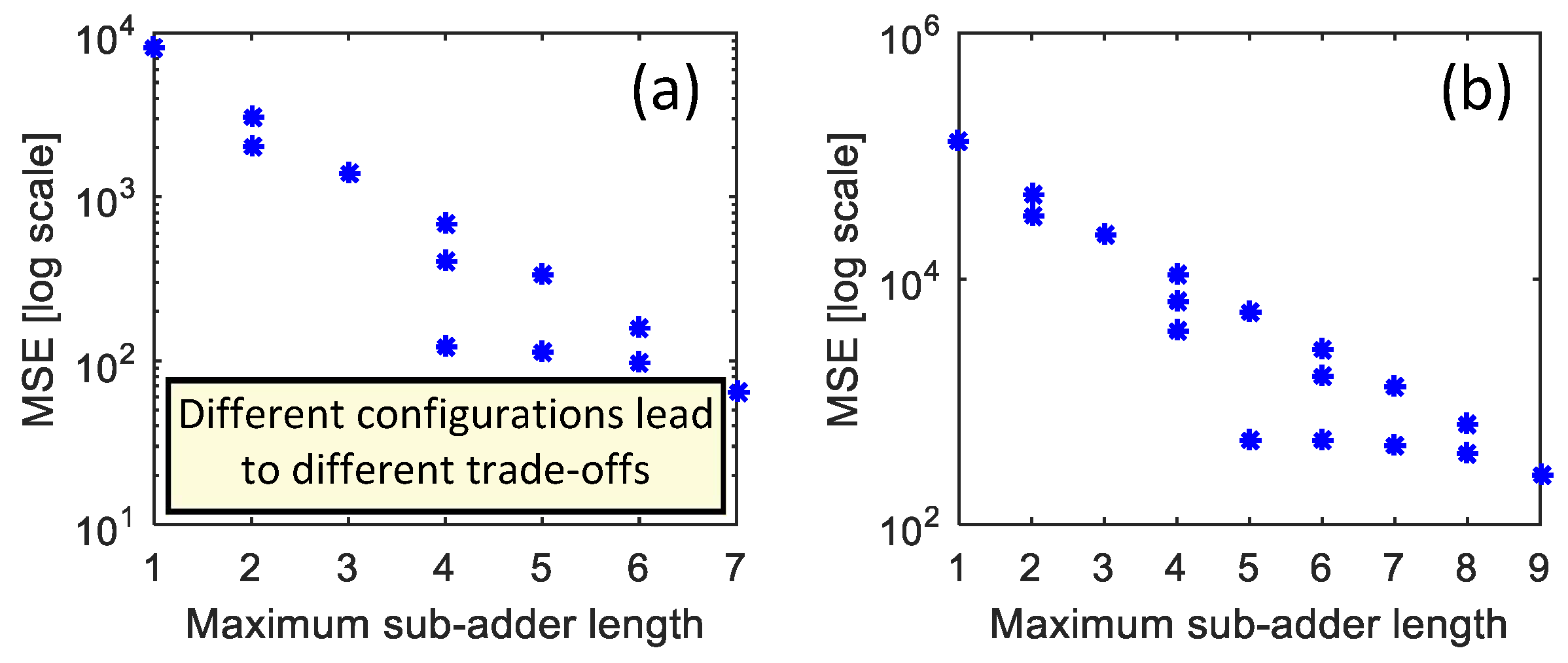
The overall design space of low-latency adders can be huge, depending on the adder length (N). For example, the design spaces of 8-bit and 10-bit low-latency adders are shown in Figure 5. Thus, the use of such high-performance approximate adders in an application demands the non-trivial task of thorough comparative evaluation due to the wide design space to assess the level of approximation incurred. A robust error analysis is thus crucial for effective design space exploration.
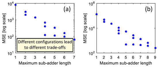
Figure 5.
Design space of low-latency approximate adders: (a) for an 8-bit adder and (b) for a 10-bit adder.
This error evaluation can be performed by using computer simulations, i.e., by simulating their functionality exhaustively or over sample data, or via analytical analysis [23]. Note that the number of simulations that have to be run is equal to the number of adder variants/configurations being evaluated. While simulations allow data- and application-specific error analysis, the requirement of extended execution time renders them unsuitable as the adder size increases [23]. Below, we provide details of DAEM, our data- and application-aware error analysis methodology for low-latency approximate adders.
3. Motivational Case Study for Analysis of the Impact of Application and Data on the Error Characteristics of Approximate Adders
In order to investigate the impact of the data and application on error analysis, we consider two image/video processing applications with comparable workloads: a low-pass filtering application with a 4 × 4 smoothing kernel and a template matching application with a template size of 4 × 4. Both applications require addition operations involving 16 values, which can be realized using approximate adders.
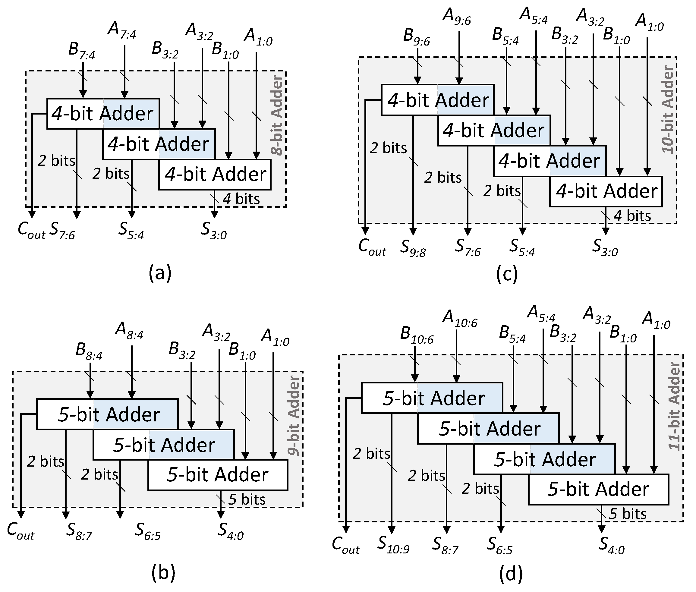
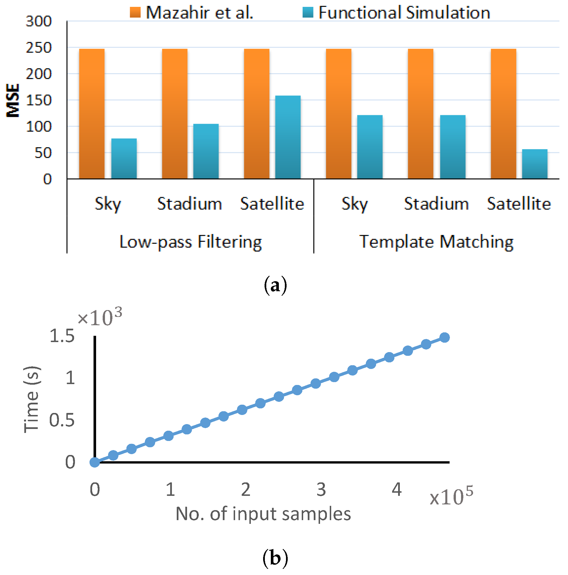
Depending upon the intended use case and deployment environment of the application system, the data input to these two applications may have some specific characteristics. As an example, here, we evaluate these two applications for three different types of input data: satellite imagery, sports stadium surveillance and sky images. Note that, irrespective of the input distribution, the low-pass filtering application requires the accumulation of data that come from the pixel’s neighborhood, which are usually highly correlated due to the spatial locality of the pixels. This is different from the template matching application, in which the sum is computed on the absolute difference, and, hence, the data are mostly uncorrelated. For the motivational analysis, we make use of a state-of-the-art generic approximate adder model called GeAr [32], as it is open source and covers various other state-of-the-art approximate adders. Depending on the number of prediction bits (P) and resultant bits (R), an N-bit GeAr adder, GeAr(N,R,P), can provide various accuracy levels, as shown in Figure 5. Assuming parallel cascaded addition, we require 4 stages of adders to compute the final sum. We built an accelerator using GeAr(8,2,2) for the first-stage additions, GeAr(9,2,3) for the second-stage additions, GeAr(10,2,2) for the third-stage additions and GeAr(11,2,3) for the final-stage addition. The adder configurations are illustrated in Figure 6. These different variants were employed to handle the bit growth across different adder stages. We use the MSE to evaluate the error introduced due to approximation. Figure 7 compares the MSE computed by using the analytical model of Mazahir et al. [23] when deploying these approximate adders in the two applications. It can be observed that since the technique proposed by Mazahir et al. [23] considers uniform uncorrelated data, the MSE turns out to be a constant value. On the contrary, for the same dataset, simulations show different error estimates for different applications. Thus, consideration of the data correlation for error estimation cannot be ignored. Similarly, for the same application, different MSEs are reported for different data types. Thus, the input data distribution needs to be considered for the error analysis of approximate adders.
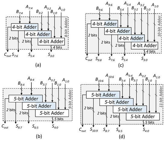
Figure 6.
The structure of different GeAr adder configurations. (a) GeAr(8,2,2); (b) GeAr(9,2,3); (c) GeAr(10,2,2); (d) GeAr(11,2,3).
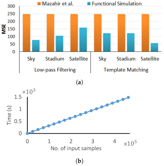
Figure 7.
(a) Comparison of the MSE evaluated using functional simulations and the MSE evaluated using the analytical model proposed by Mazahir et al. [23] (assuming uniform input distribution). (b) Execution time of functional simulations for template matching application as a function of number of input samples.
Apart from considering the input data distribution, there is also a need to consider the time required to compute the error estimates. Therefore, we also analyzed the time required to compute error measures using functional simulations, i.e., exhaustive Monte Carlo simulations using actual input samples, as well as the analytical method proposed by Mazahir et al. [23]. Figure 7 shows that although the functional simulations provide realistic error estimates as compared to the analytical method proposed by Mazahir et al. [23], the execution time for functional simulations is significantly higher than that of the analytical method, which requires only seconds to compute the error estimates for one configuration set.
In summary, we make the following key observations from the above motivational analysis:
- In real-world applications, such as a simple low-pass filtering application, the bits and operands to arithmetic components may be correlated. Thus, any assumption that violates this condition can result in significant deviation from the realistic/accurate results.
- Although functional simulations provide realistic estimates compared to the state-of-the-art error estimation techniques, their execution time is significantly longer than that for analytical methods. Thus, functional simulations cannot be used to explore a large design space in a reasonable amount of time.
Target Research Problem: As mentioned in the above case study, there is a direct need for an analytical methodology for the fast-yet-accurate error estimation of approximate adders that can leverage the data and application knowledge to provide realistic (i.e., accurate in real-world settings) error estimates in a reasonable amount of time. Moreover, the methodology should be generic enough to be applicable for a wide variety of approximate adders, so that it can allow application engineers to perform effective comparative evaluation for various adder configuration sets.
4. DAEM: Data- and Application-Aware Error Analysis Methodology
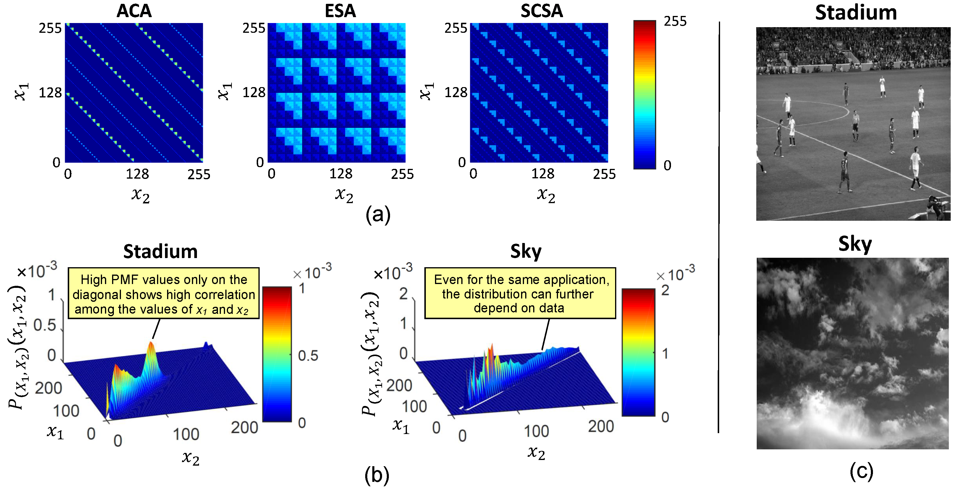
To develop an efficient data- and application-aware error analysis methodology, we first analyze the error responses of some of the approximate adders. For our analysis, we consider three types of adders, namely the ACA [29], the ESA [37] and the SCSA [38], representing three dominant classes of approximate adders, as presented in the survey by Jiang et al. [28]. We analyze the error introduced by these adders as a function of the input operands. Figure 8a provides the error maps (s) for a few notable 8-bit configurations from the aforementioned approximate adder classes. We compute the for an approximate adder by populating the error values for each possible input combination. Here, and are the two adder operands. It can be observed that the error varies as a function of the joint input combination, and not as a function of a single operand. Next, we analyze the effect of the application and the input data distribution on the 2D joint input PMF. In Figure 8b, we illustrate two sample joint probability distributions generated by using input data from two visually different sets of grayscale images (shown in Figure 8c) for a low-pass filtering application. These distributions highlight that not all the input combinations are equally likely to occur in practical data. Specifically, for applications that process the data from the spatial neighborhood of pixels, the joint input probability distribution shall be highly correlated, as shown in Figure 8b. On the contrary, for applications that process data from independent sources, the joint input probability distribution shall be independent. Thus, a 2D joint input probability distribution provides the data- and application-specific knowledge required to develop a realistic error analysis methodology. In the next section, we develop an error estimation model for a two-operand adder using its 2D input PMF. The model shall later be extended for a cascade of approximate adders.

Figure 8.
(a). Example for 8-bit ACA with , ESA with and SCSA with . The white-colored locations in represent no error. (b) Joint input probability distribution generated using neighboring pixels of two visually different sets of grayscale images shown in (c).
4.1. Error Estimation for an Approximate Adder
We define the input–output model of a standalone approximate adder, adding two operands and , as follows:
Here, represents approximate addition, y is the accurate sum and is the error in the output that is contributed by the approximate addition. Let be the 2D joint PMF representing the application-aware data dependence of the two operands of an approximate adder, where is defined as
Let be the probability distribution of the error generated due to the approximate addition of the inputs and . is defined as
can be computed by utilizing and the pre-computed of the specific approximate adder being used, as explained in Algorithm 1. In particular, is computed by looking up for all the possible error values (0 to for an n-bit adder) and summing the probabilities of all input combinations that result in the same error value. can either be provided by the application engineer or populated by logging the operand values at the inputs of the adder, assuming accurate addition.
For a standalone approximate adder unit with error-free inputs, the error generated by the adder itself is the only source of error, and, hence, the of the output error () is given by
| Algorithm 1 Procedure for computation of for a single approximate adder |
| Inputs: i.e., error map of a specific adder AND , i.e., the joint PMF of inputs of a specific adder |
| Outputs: , i.e., PMF of error generated |
|
4.2. Error Estimation for an Intermediate Approximate Adder
To develop a scalable error analysis methodology that could also be extended for cascaded addition, we now consider an approximate adder that can be located anywhere within a cascade of adders. This is illustrated in Figure 9a, where Adder 3 is adding the outputs of Adder 1 and Adder 2. Note that the inputs to Adder 3 are not only the two operands ( and ) but also the error outputs ( and ) coming from the previous adders. Therefore, the error output from Adder 3 is contributed by two error terms.
- Error generated by Adder 3 itself, with a distribution characterized by . Note that can be computed by using the data- and application-aware joint input in Algorithm 1.
- Error propagated to Adder 3 that originates from the error in the input operands ( and ), with the distribution defined by . Note that is estimated by convolving the input error PMFs, assuming the inputs to be independent of each other, similar to the assumption considered in [39]. Thus,
Here , represents the of the propagated error for Adder 3; and correspond to the of the error generated by Adder 1 and Adder 2, i.e., the inputs of Adder 3 in Figure 9; and ’∗’ represents the convolution operator. Assuming the generated and propagated errors to be independent of each other, the for the cumulative output error for Adder 3 is computed by
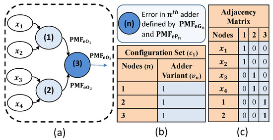
Figure 9.
(a) Error generated and propagated by an nth adder. Figure is illustrated for , i.e., the 3rd adder, which is adding the sums obtained from the 1st and 2nd adders. (b) A configuration set is defined by the type of approximate adder (adder variant) being used at each adder node. In the illustrated example of (a), each adder of the four-operand addition is using the same adder variant. Thus, the adder variant 1 is being used for each adder ((1), (2) and (3)). (c) Adjacency matrix provides the connectivity of the adder nodes.

The estimated output error distribution at each adder node n, i.e., , can be utilized to compute the required error metrics, such as MSE and MED, using the following equations.
Here, represents the magnitude vector of , represents the corresponding probability vector of and ‘.’ represents the dot product operation.
The above analysis provides error measures for an intermediate approximate adder placed within a large cascaded adder unit. Since careful design space exploration requires the evaluation of multiple approximate adder variants for each adder node, the problem at hand is to devise an effective methodology that provides a systematic method of estimating the cumulative error, due to approximation, at the output of the adder unit.
4.3. Methodology
Building upon our probabilistic error analysis, presented in Section 4.1 and Section 4.2, we provide a methodology for data- and application-aware error analysis, DAEM, for an application kernel comprising an adder unit summing N operands. Such a unit requires (N − 1) adders to compute the final sum. DAEM allows any adder variant (from the supported adders) to be evaluated for each of the (N − 1) adders. Note that, for an evaluation that involves V adder variants, a total of configurations are possible. Thus, a tth configuration set, , can be specified by an array, =,,…,, where and represents the adder variant of the ith adder, with .
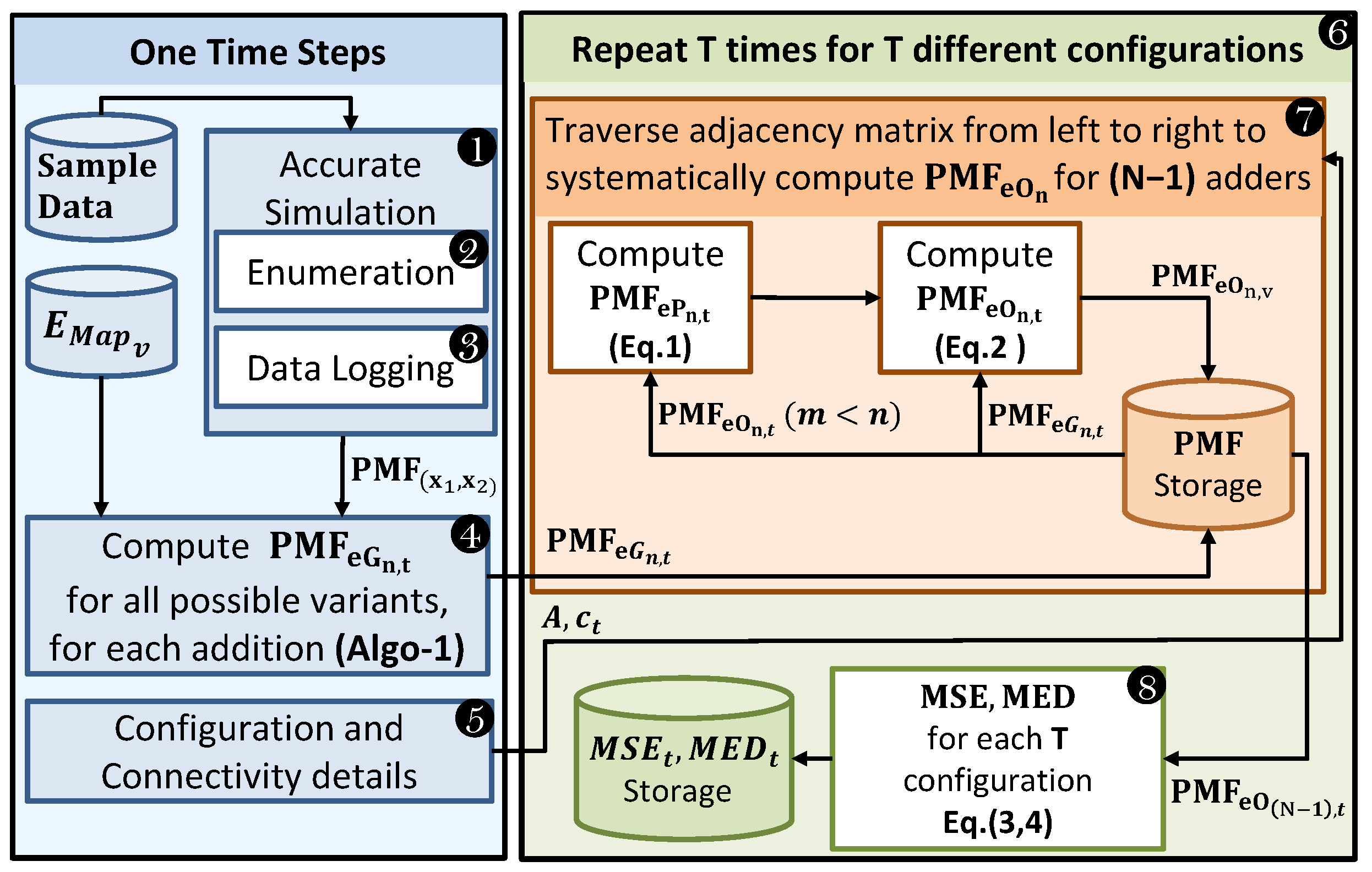
For the example case of Figure 9, we assumed V = 1, and, therefore, there was only one configuration (T = 1), with all adders of the same variant/type, and hence = . Thus, an adder within a configuration t is uniquely represented by , where n defines its enumerated location and provides its variant number. Our DAEM methodology requires sample data, application code, and error maps of the V approximate adder variants, and it provides an estimate of the error metrics (error PMF, MSE and MED) for all the T configuration sets. Figure 10 illustrates the different steps involved in DAEM, which are discussed below.
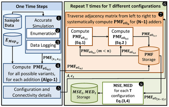
Figure 10.
Proposed data- and application-aware error analysis methodology for approximate adders.
First, an accurate simulation of the application kernel being approximated must be conducted using realistic sample data (Step 1). This is justified since application engineers typically perform accurate simulations for the functional evaluation of their code using some testing/sample data. DAEM requires accurate simulation code for the application with two trivial modifications. Firstly, a code snippet is added that enumerates the adders from 1 to N − 1 (Step 2 in Figure 10), in the order of their execution in the software, and assigns them a node ID (an example is illustrated in Figure 9a). These node IDs are later used in Step 5 to generate an adjacency matrix (A), similar to the one shown in Figure 9c. Secondly, as the accurate simulation runs, the inputs to each adder have to be logged (Step 3) to compute the 2D joint input PMF, , associated with each nth adder. In Step 4, these logged data allow us to generate , the of the error generated by the nth adder of the tth configuration set, as explained in Section 4.1. The adjacency matrix (A) defining the connectivity of the adders, their associated and the list of configuration sets to be evaluated are provided to Step 6, which runs T times to compute the error metrics for T configurations. For each configuration set, the adjacency matrix (A) is traversed column-wise, from left to right, and is evaluated (Step 7). , the error of the (N − 1)th node, defines the of the error at the output of the accelerator, and, hence, it is used in Step 8 to compute the cumulative and of the tth configuration set. Note that Step 6 is repeated for all the configuration sets.
5. Results and Discussion
In this section, we provide the evaluation results of our DAEM methodology for multiple application scenarios. These include a few cases of synthetic application/data and a few representative kernels from image, audio and video processing. For each of these cases, the estimated error measures ( [22] and [40]) are compared with those obtained from the state-of-the-art analytical model of [23], as well as with those obtained using functional simulations performed using MATLAB. For our analysis and results, we employ different variants of the GeAr [32] adder, as it is a well-cited and generic model that captures the functionality of the majority of the prominent state-of-the-art approximate adders, including ACA-I, ACA-II, ETAII and different variants of GDA. Furthermore, it is also available as an open-source library and, hence, allows reproducible comparisons. The analytical model of [23], the proposed DAEM methodology and the exhaustive simulation code were all implemented in MATLAB for evaluation.
5.1. Comparison with State-of-the-Art [23]
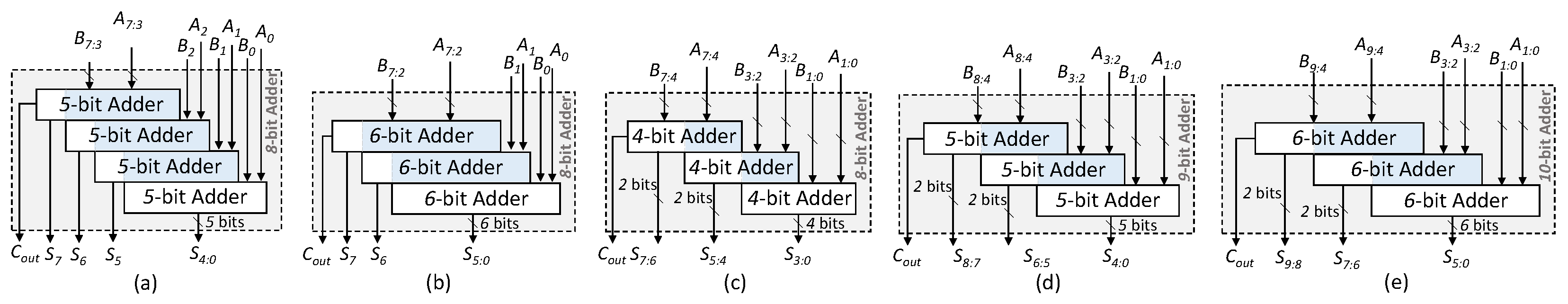
First, we evaluate the accuracy of the error metrics estimated using DAEM for synthetic data, similar to the evaluation experiments performed by Mazahir et al. in [23] for their analytical scheme. Error metrics were evaluated for a single adder accelerator, for five different configuration sets (T = 5). The adder variants considered for this evaluation were GeAr(8,1,4), GeAr(8,1,5), GeAr(8,2,2), GeAr(9,2,3) and GeAr(10,2,4). The configurations are shown in Figure 11.

Figure 11.
The configurations of the GeAr adder model used for evaluation using synthetic data. (a) GeAr(8,1,4); (b) GeAr(8,1,5); (c) GeAr(8,2,2); (d) GeAr(9,2,3); (e) GeAr(10,2,4).
Three different input distributions were evaluated:
- (1)
- Uniformly distributed uncorrelated inputs;
- (2)
- Uncorrelated Gaussian distribution with and ;
- (3)
- Correlated Gaussian distribution with and .
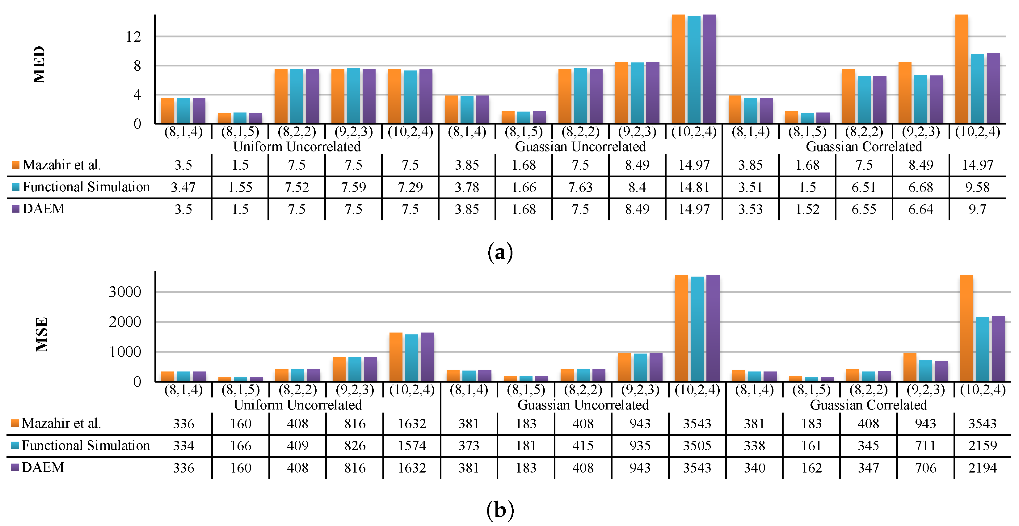
Figure 12 provides a comparison of the estimated error measures computed using DAEM and the analytical scheme of [23], for all three input distributions. Since DAEM makes use of 2D PMFs, these distributions were directly employed to compute the error PMF, MSE and MED. However, since the analytical model of [23] can use only 1D PMF, we employed the marginal PMF of each of these three distributions as its input. To provide a fair comparison, we further performed the accurate but rather time-consuming Monte Carlo simulations. For this, we generated a 100,000-point dataset for each of the above three distributions and performed functional simulations for each of the GeAr adder configurations. The MSE and MED were then computed by comparing them against the accurate addition results.
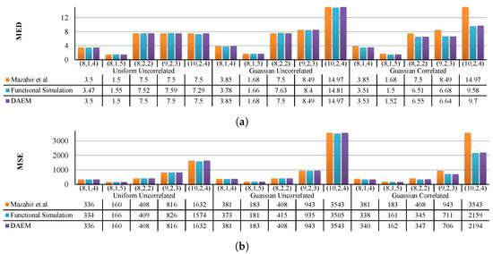
Figure 12.
Comparison of DAEM, state-of-the-art Mazahir et al. [23] and functional simulation results ( and ) obtained using 5 different configurations of GeAr for three different data distributions. Each GeAr configuration is represented in its generic form (N, R, P). The figure clearly shows that for uncorrelated data case, both the proposed and the state-of-the-art methods provide accurate estimates, and for the correlated case, the DAEM methodology provides better estimates than SOTA.
The estimated measures of the MED (Figure 12a) and MSE (Figure 12b) for both the uncorrelated input distributions illustrate that the proposed model has performance equivalence to that of the state-of-the-art [23]. In fact, the error estimated by both DAEM and [23] matches closely with that of the functional simulation results for uncorrelated input distributions. However, as illustrated in the previous sections, in real-world applications, the inputs of adders are typically correlated and resemble the Gaussian correlated distribution. For correlated inputs, we see that DAEM provides an accurate estimate of the MSE and MED for all the configurations. This is unlike [23] that fails to provide an accurate error estimate. Thus, the proposed model outperforms the state-of-the-art techniques by taking maximum advantage of the joint input distribution.
Next, we utilize real-world data to demonstrate that DAEM provides better estimates of the error measures as compared to the state-of-the-art techniques. Similar to the motivational analysis of Figure 7, we compare the MSE values, estimated for two different applications, for three different datasets and provide the results in Figure 13. Applications considered were low-pass filtering using a 4 × 4 kernel and template matching using a 4 × 4 kernel. The parallel adder accelerator used for this analysis utilized a configuration set with four different adder variants: GeAr(8,2,2) for the first-stage additions, GeAr(9,2,3) for the second-stage additions, GeAr(10,2,2) for the third-stage additions and GeAr(11,2,3) for the final-stage addition. The dataset contained 30 images (10 per class) of landscapes, which were collected using Google Images and Google Maps and classified as Sky, Stadium and Satellite, depending on their content. For DAEM, we computed the required 2D input joint PMFs using five images from the corresponding class. To compute the ground truth, functional simulations were performed in MATLAB using the rest of the five images for each class. In Figure 13, we report the MSE estimates for both DAEM and the state-of-the-art [23], compared to the MSE computed using functional simulations. It can be observed that for both the applications and all three datasets, the MSE estimated using DAEM is more realistic as compared to the estimates computed using the state-of-the-art [23]. It can also be observed from the figure that the error estimates provided using DAEM follow the same trend as that of the functional simulations. Thus, we conclude that DAEM provides better estimates of the error measures as compared to the state-of-the-art techniques.
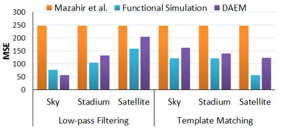
Figure 13.
Comparison of error in estimated MSE generated using DAEM, state-of-the-art by Mazahir et al. [23], and simulation results for two image processing applications for three datasets.
Although the error measures computed using DAEM provide a better estimate as compared to the state-of-the-art, the estimated MSE still does not exactly match that of the functional simulations. This can be attributed to two reasons.
- Errors in the adders that are located in the earlier stages may trigger changes in the joint input PMFs of some/all the adders in the subsequent stages. However, as the variations in the joint input PMFs of low-latency adders are expected to be either small in magnitude or less frequent, and capturing these variations requires a significant amount of computation, to keep the model lightweight, these variations are ignored.
- The joint input PMFs of the adders for the testing set (i.e., the set used to perform functional simulations) can be different from the ones used for training (i.e., for data logging—Step-3 in Figure 10—in the DAEM methodology). These variations will further be discussed and analyzed in Section 5.2 and Section 5.3 for audio and video processing applications, respectively.
5.2. DAEM in Audio Processing
To illustrate the applicability of the proposed methodology in a different real-world application (i.e., other than image/video processing applications), we employed DAEM in an audio low-pass filtering application.
The dataset used for evaluation in this section comprises audio files from a standard audio dataset used for the human activity recognition application [41] and raw 8-bit audio files from http://www.class-connection.com/8bit-ulaw.htm (accessed on 1 January 2019). The raw audio files are included to show the effectiveness of DAEM even for real-life data. To reduce the overall simulation time of the experiment, we used a subset of the complete dataset. We used 100 audio files from the human activity recognition dataset along with 16 raw 8-bit audio files, which were randomly selected from the individual sets. The files were then converted to 8-bit format with a sampling frequency of 8 kHz to maintain uniformity in the audio files so that the same functional model could be used for simulations.
To highlight the importance of the selection of data for data logging in DAEM and to illustrate the applications for which DAEM is suited, we considered two different scenarios.
- Random Selection: The audio files were randomly divided into two groups. One of these groups was employed as training data for data logging (Step 3) in the DAEM methodology.
- Guided Selection: Each audio file was split into two parts. A new group of files was formed comprising the first half of these audio files, and it was used as the training data for data logging (Step 3) in the DAEM methodology.
In both the aforementioned scenarios, the second group of files (hereinafter referred to as the testing set) was used to compute error measures using functional simulations.
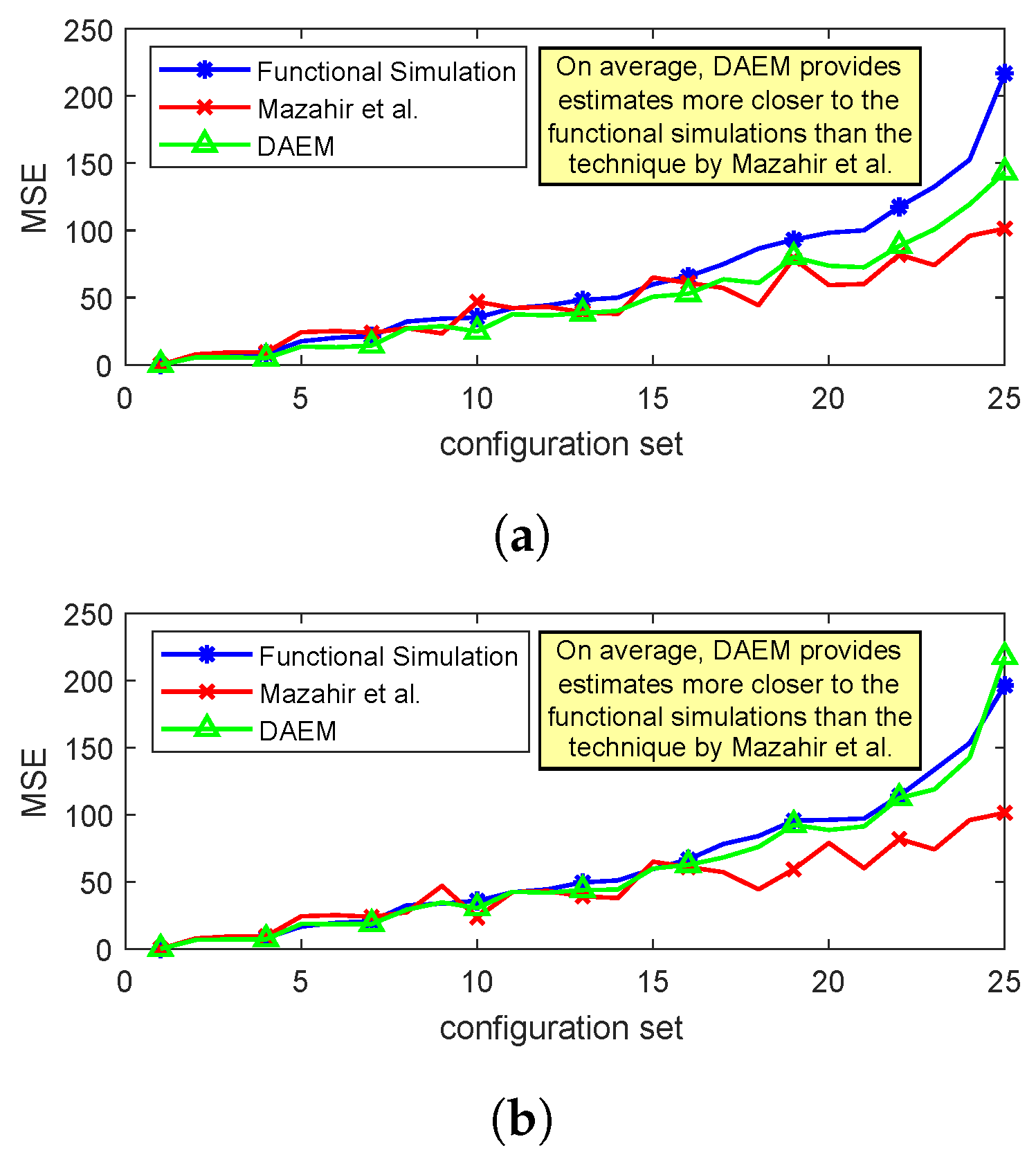
Figure 14a,b provides a comparison of the proposed and the state-of-the-art techniques with the simulation results for the two aforementioned scenarios. For the presented example case, the audio low-pass filtering application is implemented using a moving-average filter having a frequency response . The results were generated for 25 different configuration sets (T = 25), which were then sorted based on the MSE values of the functional simulation results and then plotted. The figures illustrate that, in both the scenarios, DAEM provides realistic error estimates as compared to the state-of-the-art technique. It can also be observed (Figure 14b) that DAEM provides an even better estimate for the scenario where we performed a guided selection of training data. This increased level of estimation accuracy of DAEM for the “guided selection” scenario can be attributed to the correlation between the training dataset and the testing dataset.
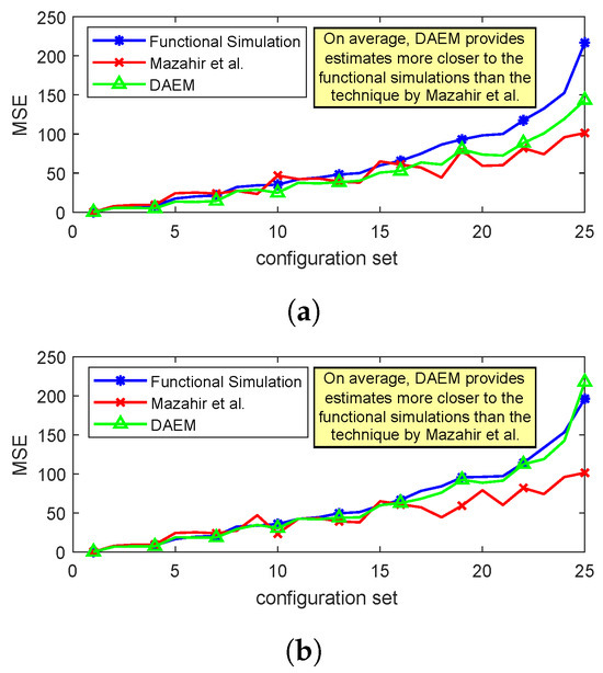
Figure 14.
Comparison of DAEM with state-of-the-art [23] and simulation results for audio low-pass filtering application. (a) Scenario 1 and (b) Scenario 2.
In short, it can be concluded that, in particular, DAEM provides error measures that are close to the ones obtained using simulation results when the training data are carefully selected and are hence appropriately representative of the input data.
5.3. DAEM in Video Processing
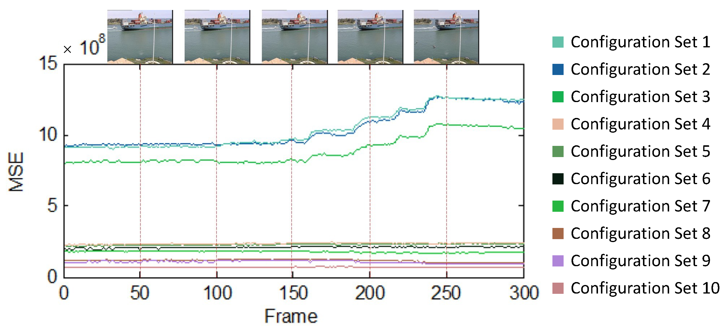
Videos captured in a static setting, such as surveillance videos, provide a common use case where the background is mostly static, and, hence, the overall visual information in each frame is almost the same. Due to this, a portion of the video acquired from such a static camera provides a good representative sample for the video and is hence highly suitable to be used as the training data for our DAEM methodology. Thus, the error measures predicted by DAEM over the training dataset are expected to stay consistent in the testing data. To illustrate this, we applied a 4 × 4 average filtering on each frame of a video. We used the container video, which is a standard video from the video processing domain and is available at http://trace.eas.asu.edu/yuv/ (accessed on 1 January 2019). The video was captured using a statically placed camera. We evaluated the per frame for 10 configuration sets (T = 10), for a total of 300 frames. Each colored plot/graph in Figure 15 represents the estimated for each configuration set for the input frames. It can be observed that the relative standing of for each configuration set is mostly consistent. Thus, DAEM can be efficiently employed to rank the suitability of a configuration set for approximation. DAEM can further be employed to perform design space exploration and, hence, aid in the selection of the most suitable configuration set.
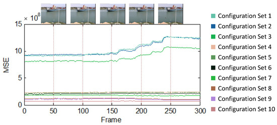
Figure 15.
Variations in per-frame MSE across frames of standard video for 4 × 4 approximate low-pass filtering application. The results are illustrated for 10 different configuration sets.
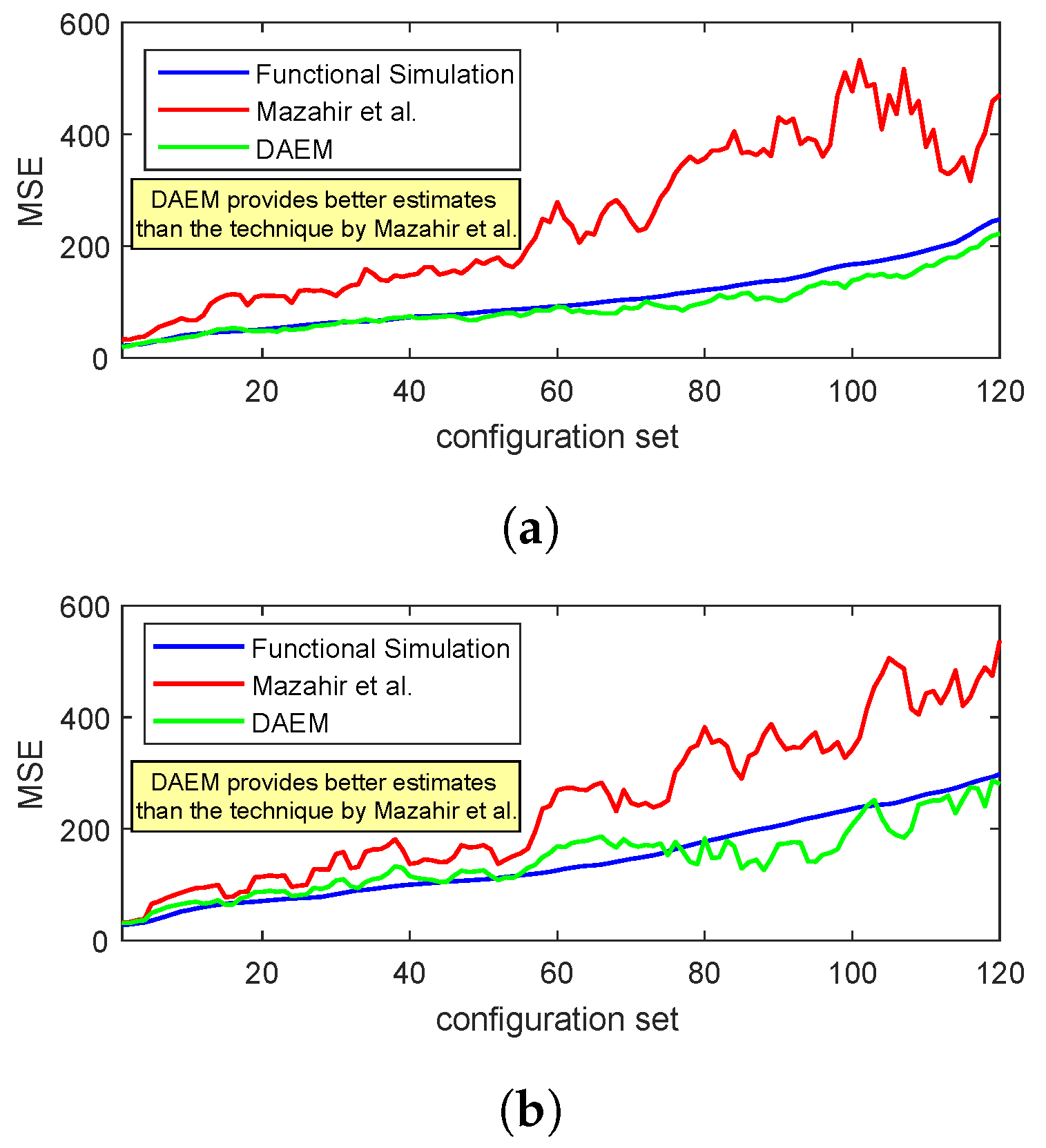
To demonstrate the efficacy of DAEM for videos, we next consider the adder unit of a 4 × 4 averaging filter. We evaluate the at the output of the filter for 120 different configuration sets (T = 120). In Figure 16, we plot the estimated using DAEM and compare it with that of the state-of-the-art [23] and functional simulations. Results are provided for two standard videos (the “container” and the “coastguard” videos), which are used frequently for benchmarking in the video coding domain. The training set used for the proposed method was the five initial frames of the video, and the simulation results were generated using the following 20 frames. The results were generated for 120 randomly selected configuration sets, which were then sorted based on the MSE values of the simulated results and then plotted. It can be observed that the results of the proposed methodology are almost in complete accordance with the simulated results and provide better trend following as compared to the state-of-the-art technique.
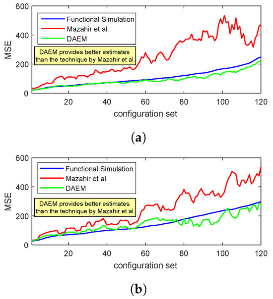
Figure 16.
Comparison of DAEM with state-of-the-art Mazahir et al. [23] and simulated results for a 4 × 4 low-pass filtering application for two standard videos: (a) container, (b) coastguard.
6. Evaluation of the Time Requirements for the Error Estimation Effort
In this section, we analyze the timing performance of our DAEM methodology. DAEM comprises two main computing blocks, as illustrated in Figure 10.
- The first block is required to be executed only once and comprises Steps 1–5. It is assumed that s are pre-calculated, since they are only dependent on the adder variant/type. Accurate simulation comprising enumeration and data logging takes most of the time in this block.
- The second block (Steps 6–8) is executed T number of times to estimate the performance of each configuration set. However, these steps have a low computational cost.
Table 1 presents the time taken by DAEM and the methodology proposed by Mazahir et al. [23] and compares it with the time taken by exhaustive simulations for the low-pass filtering application results of Figure 16. For this comparison, we evaluated the results for 120 different configuration sets (i.e., T = 120). It can be observed from the table that DAEM takes significantly (around 3000×) less time compared to exhaustive simulations. This is mainly because, unlike exhaustive simulations, which must be performed for all the T configuration sets, DAEM only requires accurate simulation (i.e., execution of Steps 1–5) once, and on only a relatively small training dataset. For our evaluation, Steps 1–5 take only 71.687 s for execution, and Steps 6–8, which are repeated T times (once for each configuration set), take only 0.073 s for execution. Note that, as for larger design spaces, i.e., larger T values, the execution time for design space exploration is dominated by Steps 6–8. By comparing the computational efficiency of Steps 6–8 of DAEM with that of the methodology proposed by Mazahir et al. in [23], we can conclude that DAEM offers computational efficiency comparable to that of Mazahir et al. [23].

Table 1.
Timing comparison of error estimation schemes with simulations (s).
7. Discussion of Limitations and Future Work
Note that the scalability of DAEM can be limited in certain cases, depending on the following two factors.
- Hardware accelerators are usually composed of cascaded stages where the inputs are fed to computing modules in the first stage and the output of the first stage is used as input to the second stage and so on. As the number of cascaded stages increases, the estimation of the joint input probability distribution of the computing modules becomes less accurate. This is because approximations in the earlier stages cause the joint input probability distribution of the modules in the latter stages to significantly deviate from the estimated joint input probability distribution. Hence, the proposed approach is highly effective for shallow accelerators, i.e., accelerators having a smaller number of cascaded stages, but may not produce reliable results for cases where the number of cascaded stages is large.
- The number of possible input combinations of a computing module increases exponentially with the increase in its input bit-width. This translates to huge memory requirements for the error maps and joint input probability distribution of the larger modules. For example, to store an error map of an 8-bit approximate adder in 8-bit integer format, a total of bytes (i.e., 64 KB) of memory is required; however, for a 16-bit adder, the memory requirement translates to bytes (i.e., 4 GB).
These limitations can potentially be addressed using the following future directions.
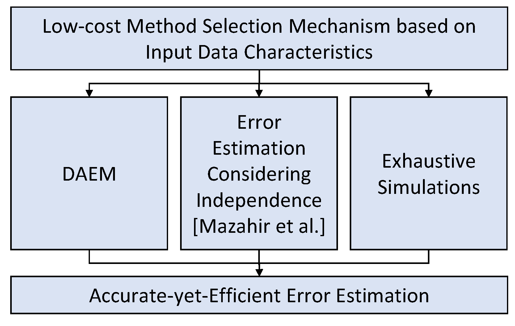
- One future direction can be building a holistic framework by integrating multiple different existing tools that offer a better accuracy–execution time trade-off in different scenarios and use a simple method/tool selection mechanism at the start to decide the most appropriate tool based on the input data characteristics and the given data path. For example, we can combine DAEM with simple convolution-based methods such as [23] and exhaustive simulations to build a framework that can offer an improved accuracy–execution time trade-off for a wide range of scenarios. However, such a framework requires thorough analysis to identify the strengths and weaknesses of different techniques, which can help in designing a low-cost selection mechanism. A high-level conceptual illustration of such a tool is presented in Figure 17.
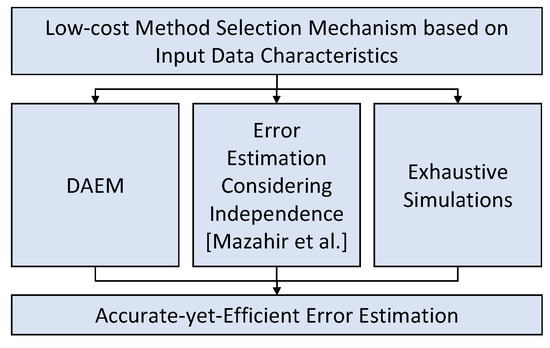 Figure 17. Accurate-yet-efficient error estimations based on integration of multiple error estimation techniques that outperform others under certain specific conditions.
 - Another possible direction in addressing the limitations of the proposed approach is to explore machine learning to learn the dynamics of error propagation and masking in a data path and use the learned model to offer improved error estimation, especially for deeper data paths.
8. Conclusions
In this work, we analyzed the impact of commonly employed assumptions in error estimation techniques designed for approximate adders on their accuracy. The analysis highlighted that there is a need to relax these assumptions to achieve better results. Therefore, in this paper, we propose an data- and application-aware error estimation methodology (DAEM) to evaluate the error of approximate adders. The methodology provides an estimate of the probability mass function (PMF) of the output error along with estimates for the mean squared error (MSE) and mean error distance (MED). The methodology is applicable to a large number of state-of-the-art adders, such as GeAr, ACA and GDA. The experimental results suggest that, unlike state-of-the-art techniques, the proposed methodology provides accurate results for synthetic correlated data and also provides error estimates that closely follow the trend of exhaustive simulations for real-world applications. Compared to the state-of-the-art techniques, DAEM provides better error estimates in representative audio and video processing applications that have a consistent input probability distribution over time.
Author Contributions
Conceptualization, methodology and writing—original draft preparation: all authors. Software, validation, investigation, data curation and visualization: M.A.H. All authors have read and agreed to the published version of the manuscript.
Funding
This research is supported by ASPIRE, the technology program management pillar of Abu Dhabi’s Advanced Technology Research Council (ATRC), via the ASPIRE Awards for Research Excellence, for the proposal “Towards Extreme Energy Efficiency through Cross-Layer Approximate Computing”. The coauthor Dr. Rehan’s contributions in this work are partially supported by the Higher Education Commission (HEC) of Pakistan, under NRPU project # 10150, titled, “AxVision—Application Specific Data-Aware, Approximate-Computing for Energy Efficient Image and Vision Processing Applications”.
Data Availability Statement
Data sharing not applicable.
Conflicts of Interest
The funders had no role in the design of the study; in the collection, analyses, or interpretation of data; in the writing of the manuscript.
References
- Han, J.; Orshansky, M. Approximate computing: An emerging paradigm for energy-efficient design. In Proceedings of the 2013 18th IEEE European Test Symposium (ETS), Avignon, France, 27–30 May 2013; pp. 1–6. [Google Scholar]
- Venkataramani, S.; Chakradhar, S.T.; Roy, K.; Raghunathan, A. Approximate computing and the quest for computing efficiency. In Proceedings of the 52nd Annual Design Automation Conference, San Francisco, CA, USA, 8–12 June 2015; pp. 1–6. [Google Scholar]
- Mittal, S. A survey of techniques for approximate computing. ACM Comput. Surv. (CSUR) 2016, 48, 1–33. [Google Scholar] [CrossRef]
- Stanley-Marbell, P.; Alaghi, A.; Carbin, M.; Darulova, E.; Dolecek, L.; Gerstlauer, A.; Gillani, G.; Jevdjic, D.; Moreau, T.; Cacciotti, M.; et al. Exploiting errors for efficiency: A survey from circuits to applications. ACM Comput. Surv. (CSUR) 2020, 53, 1–39. [Google Scholar] [CrossRef]
- Xu, Q.; Mytkowicz, T.; Kim, N.S. Approximate computing: A survey. IEEE Des. Test 2015, 33, 8–22. [Google Scholar] [CrossRef]
- Mishra, A.K.; Barik, R.; Paul, S. iACT: A software-hardware framework for understanding the scope of approximate computing. In Proceedings of the Workshop on Approximate Computing across the System Stack (WACAS), Salt Lake City, UT, USA, 2 March 2014. [Google Scholar]
- Nair, R. Big data needs approximate computing: Technical perspective. Comm. ACM 2015, 58, 104. [Google Scholar] [CrossRef]
- Bornholt, J.; Mytkowicz, T.; McKinley, K.S. Uncertain <T>: Abstractions for uncertain hardware and software. IEEE Micro 2015, 35, 132–143. [Google Scholar]
- Bornholt, J.; Mytkowicz, T.; McKinley, K.S. Uncertain <T>: A first-order type for uncertain data. In Proceedings of the 19th International Conference on Architectural Support for Programming Languages and Operating Systems, Salt Lake City, UT, USA, 1–5 March 2014; Volume 49, pp. 51–66. [Google Scholar]
- Misailovic, S.; Carbin, M.; Achour, S.; Qi, Z.; Rinard, M.C. Chisel: Reliability-and accuracy-aware optimization of approximate computational kernels. ACM SIGPLAN Not. 2014, 49, 309–328. [Google Scholar] [CrossRef]
- Zhu, N.; Goh, W.L.; Zhang, W.; Yeo, K.S.; Kong, Z.H. Design of low-power high-speed truncation-error-tolerant adder and its application in digital signal processing. IEEE Trans. Very Large Scale Integr. (VLSI) Syst. 2009, 18, 1225–1229. [Google Scholar]
- Taylor, M.B. Is dark silicon useful? Harnessing the four horsemen of the coming dark silicon apocalypse. In Proceedings of the DAC Design Automation Conference 2012, San Francisco, CA, USA, 3–7 June 2012; pp. 1131–1136. [Google Scholar]
- Wijtvliet, M.; Waeijen, L.; Corporaal, H. Coarse grained reconfigurable architectures in the past 25 years: Overview and classification. In Proceedings of the 2016 International Conference on Embedded Computer Systems: Architectures, Modeling and Simulation (SAMOS), Samos, Greece, 18–21 July 2016; pp. 235–244. [Google Scholar]
- Karunaratne, M.; Mohite, A.K.; Mitra, T.; Peh, L.S. Hycube: A cgra with reconfigurable single-cycle multi-hop interconnect. In Proceedings of the 54th Annual Design Automation Conference 2017, Austin, TX, USA, 18–22 June 2017; pp. 1–6. [Google Scholar]
- Peng, G.; Liu, L.; Zhou, S.; Yin, S.; Wei, S. A 2.92-Gb/s/W and 0.43-Gb/s/MG Flexible and Scalable CGRA-Based Baseband Processor for Massive MIMO Detection. IEEE J. Solid-State Circuits 2020, 55, 505–519. [Google Scholar] [CrossRef]
- Akbari, O.; Kamal, M.; Afzali-Kusha, A.; Pedram, M.; Shafique, M. Toward Approximate Computing for Coarse-Grained Reconfigurable Architectures. IEEE Micro 2018, 38, 63–72. [Google Scholar] [CrossRef]
- Ye, R.; Wang, T.; Yuan, F.; Kumar, R.; Xu, Q. On reconfiguration-oriented approximate adder design and its application. In Proceedings of the 2013 IEEE/ACM International Conference on Computer-Aided Design (ICCAD), San Jose, CA, USA, 18–21 November 2013; pp. 48–54. [Google Scholar]
- Ebrahimi-Azandaryani, F.; Akbari, O.; Kamal, M.; Afzali-Kusha, A.; Pedram, M. Block-based carry speculative approximate adder for energy-efficient applications. IEEE Trans. Circuits Syst. II Express Briefs 2019, 67, 137–141. [Google Scholar] [CrossRef]
- Sengupta, D.; Sapatnekar, S.S. FEMTO: Fast error analysis in Multipliers through Topological Traversal. In Proceedings of the 2015 IEEE/ACM International Conference on Computer-Aided Design (ICCAD), Austin, TX, USA, 2–6 November 2015; pp. 294–299. [Google Scholar]
- Ayub, M.K.; Hanif, M.A.; Hasan, O.; Shafique, M. PEAL: Probabilistic Error Analysis Methodology for Low-power Approximate Adders. ACM J. Emerg. Technol. Comput. Syst. (JETC) 2020, 17, 1–37. [Google Scholar] [CrossRef]
- Hanif, M.A.; Hafiz, R.; Hasan, O.; Shafique, M. PEMACx: A probabilistic error analysis methodology for adders with cascaded approximate units. In Proceedings of the 2020 57th ACM/IEEE Design Automation Conference (DAC), San Francisco, CA, USA, 20–24 July 2020; pp. 1–6. [Google Scholar]
- Liu, C.; Han, J.; Lombardi, F. An analytical framework for evaluating the error characteristics of approximate adders. IEEE Trans. Comput. 2015, 64, 1268–1281. [Google Scholar] [CrossRef]
- Mazahir, S.; Hasan, O.; Hafiz, R.; Shafique, M.; Henkel, J. Probabilistic error modeling for approximate adders. IEEE Trans. Comput. 2017, 66, 515–530. [Google Scholar] [CrossRef]
- Dou, Y.Q.; Wang, C.H. An Optimization Technique for PMF Estimation in Approximate Circuits. J. Comput. Sci. Technol. 2023, 38, 289–297. [Google Scholar] [CrossRef]
- Castro-Godínez, J.; Esser, S.; Shafique, M.; Pagani, S.; Henkel, J. Compiler-driven error analysis for designing approximate accelerators. In Proceedings of the 2018 Design, Automation & Test in Europe Conference & Exhibition (DATE), Dresden, Germany, 19–23 March 2018; pp. 1027–1032. [Google Scholar]
- Sengupta, D.; Snigdha, F.S.; Hu, J.; Sapatnekar, S.S. An analytical approach for error PMF characterization in approximate circuits. IEEE Trans. Comput.-Aided Des. Integr. Circuits Syst. 2018, 38, 70–83. [Google Scholar] [CrossRef]
- Wu, Y.; Li, Y.; Ge, X.; Gao, Y.; Qian, W. An efficient method for calculating the error statistics of block-based approximate adders. IEEE Trans. Comput. 2018, 68, 21–38. [Google Scholar] [CrossRef]
- Jiang, H.; Han, J.; Lombardi, F. A comparative review and evaluation of approximate adders. In Proceedings of the 25th edition on Great Lakes Symposium on VLSI, Pittsburgh, PA, USA, 20–22 May 2015; pp. 343–348. [Google Scholar]
- Verma, A.K.; Brisk, P.; Ienne, P. Variable latency speculative addition: A new paradigm for arithmetic circuit design. In Proceedings of the Conference on Design, Automation and Test in Europe, Munich, Germany, 10–14 March 2008; pp. 1250–1255. [Google Scholar]
- Kahng, A.B.; Kang, S. Accuracy-configurable adder for approximate arithmetic designs. In Proceedings of the 49th Annual Design Automation Conference, San Francisco, CA, USA, 3–7 June 2012; pp. 820–825. [Google Scholar]
- Zhu, N.; Goh, W.L.; Yeo, K.S. An enhanced low-power high-speed adder for error-tolerant application. In Proceedings of the 2009 12th International Symposium on Integrated Circuits, ISIC’09, Singapore, 14–16 December 2009; pp. 69–72. [Google Scholar]
- Shafique, M.; Ahmad, W.; Hafiz, R.; Henkel, J. A low latency generic accuracy configurable adder. In Proceedings of the 2015 52nd ACM/EDAC/IEEE Design Automation Conference (DAC 2015), San Francisco, CA, USA, 8–12 June 2015; pp. 1–6. [Google Scholar]
- Miao, J.; He, K.; Gerstlauer, A.; Orshansky, M. Modeling and synthesis of quality-energy optimal approximate adders. In Proceedings of the 2012 IEEE/ACM International Conference on Computer-Aided Design (ICCAD), San Jose, CA, USA, 5–8 November 2012; pp. 728–735. [Google Scholar]
- Stefanidis, A.; Zoumpoulidou, I.; Filippas, D.; Dimitrakopoulos, G.; Sirakoulis, G.C. Synthesis of Approximate Parallel-Prefix Adders. IEEE Trans. Very Large Scale Integr. (VLSI) Syst. 2023. [Google Scholar] [CrossRef]
- Zhu, N.; Goh, W.L.; Yeo, K.S. Ultra low-power high-speed flexible probabilistic adder for error-tolerant applications. In Proceedings of the 2011 International SoC Design Conference, Jeju, Republic of Korea, 17–18 November 2011; pp. 393–396. [Google Scholar]
- Zhu, N.; Goh, W.L.; Wang, G.; Yeo, K.S. Enhanced low-power high-speed adder for error-tolerant application. In Proceedings of the 2010 International SoC Design Conference, Incheon, Republic of Korea, 22–23 November 2010; pp. 323–327. [Google Scholar]
- Mohapatra, D.; Chippa, V.K.; Raghunathan, A.; Roy, K. Design of voltage-scalable meta-functions for approximate computing. In Proceedings of the 2011 Design, Automation & Test in Europe, Grenoble, France, 14–18 March 2011; pp. 1–6. [Google Scholar]
- Du, K.; Varman, P.; Mohanram, K. High performance reliable variable latency carry select addition. In Proceedings of the 2012 Design, Automation & Test in Europe Conference & Exhibition (DATE), Dresden, Germany, 12–16 March 2012; pp. 1257–1262. [Google Scholar]
- Leon-Garcia, A.; Leon-Garcia, A. Probability, Statistics, and Random Processes for Electrical Engineering, 3rd ed.; Pearson/Prentice Hall: Upper Saddle River, NJ, USA, 2008. [Google Scholar]
- Liang, J.; Han, J.; Lombardi, F. New metrics for the reliability of approximate and probabilistic adders. IEEE Trans. Comput. 2012, 62, 1760–1771. [Google Scholar] [CrossRef]
- Stork, J.A.; Spinello, L.; Silva, J.; Arras, K.O. Audio-based human activity recognition using non-Markovian ensemble voting. In Proceedings of the RO-MAN 2012, Paris, France, 9–13 September 2012; pp. 509–514. [Google Scholar]


Disclaimer/Publisher’s Note: The statements, opinions and data contained in all publications are solely those of the individual author(s) and contributor(s) and not of MDPI and/or the editor(s). MDPI and/or the editor(s) disclaim responsibility for any injury to people or property resulting from any ideas, methods, instructions or products referred to in the content. |
© 2023 by the authors. Licensee MDPI, Basel, Switzerland. This article is an open access article distributed under the terms and conditions of the Creative Commons Attribution (CC BY) license (https://creativecommons.org/licenses/by/4.0/).