Article

A Single-Product Multi-Period Inventory Routing Problem under Intermittent Demand

1
School of Economics & Management, Shanghai Maritime University, Shanghai 201306, China
2
Logistics Engineering College, Shanghai Maritime University, Shanghai 201306, China
3
Alibaba Business School, Hangzhou Normal University, Hangzhou 311121, China
*
Author to whom correspondence should be addressed.
Information 2023, 14(6), 331; https://doi.org/10.3390/info14060331
Submission received: 13 May 2023 / Revised: 8 June 2023 / Accepted: 9 June 2023 / Published: 12 June 2023
(This article belongs to the Section Artificial Intelligence)

Abstract

:
Demand fluctuations and uncertainty bring challenges to inventory management, and intermittent demand patterns increase the risk of inventory backlogs and raise inventory holding costs. In previous studies on inventory routing problems, different variants have been proposed to cope with complicated industrial scenarios. However, there are few studies on inventory routing problems with intermittent demand patterns. To solve this problem, we introduce a lateral transshipment strategy and build a single-product multi-period inventory routing mixed integer programming model to reduce customers’ inventory backlogs, balance regional inventory, reduce inventory holding costs, and improve inventory management efficiency. Furthermore, we design an adaptive large-neighborhood search algorithm with new operators to improve the solving efficiency. The experimental results show that an appropriate transshipment price can reduce the share of distribution costs. Another finding is that higher-capacity vehicles lead to higher revenue. Our findings not only expand the scope of the IRP domain but also provide actionable management insights for business practitioners.

1. Introduction

Inventory management is a pivotal aspect of supply chain management given its role in ensuring the availability of appropriate products at the designated location, time, and cost optimization [1,2]. However, the unpredictability of consumer demand poses significant challenges to inventory management. Sudden demand can lead to stockouts, reducing customer service levels. Conversely, a decrease in demand then creates backlogs, increasing inventory costs [3,4]. Moreover, uncertainty and variability in demand patterns can make it difficult to accurately predict future demand, which directly impacts inventory planning and replenishment decisions [5]. As a result, managers employ diverse strategies to address these fluctuations and enhance the efficacy of inventory management.
To reduce the impact of demand fluctuations on inventory management, an optional strategy is to develop appropriate inventory plans for different categories by classifying demand. The concept of demand classification based on different patterns was initially explored by Williams [6], who introduced the notion of variance partitioning to categorize demand patterns as “smooth”, “slow-moving”, or “sporadic”. Subsequently, Syntetos et al. [7] extended the research on demand classification by incorporating the square of the coefficient of variation (CV) of demand size and the average demand interval (ADI). They categorized demand patterns into four categories, including “smooth”, “lumpy”, “intermittent”, and “erratic”, based on the cutoff values of these two parameters. The intermittent demand pattern is prevalent in various fields, such as retailing, spare parts management, aerospace, and electronics. It has gained significant attention from scholars owing to its uniqueness and importance. Unlike other demand patterns, intermittent demand is characterized by a large number of zero values, and the intervals between these zero values are irregular, raising the risk of inventory backlogs [8].
A D I = T o t a l   p e r i o d s T o t a l   d e m a n d   b u c k e t s
C V = D e m a n d   s t a n d a r d   d e v i a t i o n D e m a n d   m e a n
The inventory routing problem (IRP) is an important optimization problem in inventory management that requires determining when to deliver the number of goods to a given customer and the route of the vehicle [9]. The importance of the IRP is reflected in the way it not only helps companies reduce inventory costs and the risk of stockouts but also improves the transportation efficiency of their fleets [10]. In previous research, the IRP has been studied by a large number of scholars, and different variants of the problem have been proposed. The demand significantly impacts the IRP as it directly influences routing and inventory management decisions, and the change in demand derives from deterministic and stochastic variants of the IRP. The intermittent demand model can be seen as a special case of stochastic demand, and the large amount of zero demand in this pattern creates inventory backlogs and raises inventory holding costs. In this context, this study aims to focus on an IRP with intermittent demand patterns. To reduce inventory costs and improve inventory management efficiency, we use a lateral transshipment strategy to address demand fluctuations.
Consider a single-product multi-period IRP with intermittent demand (IDSMIRP) in a supply chain system. This model considers a two-echelon supply chain system consisting of a central warehouse and multiple customers, with the central warehouse responsible for maintaining inventory levels for all customers. Before the start of the replenishment cycle, the central warehouse forecasts future demand based on customers’ historical demand. Using the estimated demand and customer inventory levels, the replenishment plan is initially formulated. During the replenishment cycle, the central warehouse arranges its own vehicles to determine the appropriate replenishment route based on the distance between the warehouse and each customer node. Distribution vehicles from the central warehouse complete replenishment tasks at each customer node before returning to the warehouse. When the distribution vehicles visit the customer nodes, the actual number of customer demands becomes known. In these circumstances, products can be transferred to other customer nodes through lateral transshipment, which is provided by a third-party transportation servicer. Figure 1 illustrates an example of a lateral transshipment inventory routing model.
The main contributions of this study are:
(a)
We focus on the problem of an IRP with intermittent demand patterns (IDIRP) and expand the scope of IRP research.
(b)
We introduce the lateral transshipment strategy into an IDIRP to cope with the demand fluctuations of intermittent patterns.
(c)
We develop an MIP model for the IDIRP and improve the operators of the ALNS algorithm to enhance the solution efficiency.
The remainder of the paper is organized as follows:
Section 2 provides a literature review. In Section 3, we formally introduce the IDSMIRP. Section 4 gives detailed information about the ALNS algorithm. In Section 5, we conduct the case study. The conclusions are presented in Section 6.

2. Literature Review

The IRP is a distribution problem in which a product must be shipped from a supplier to several customers over a given time horizon. The IRP is based on the vehicle routing problem (VRP) and considers inventory management at the customer point. The VRP was first proposed by Dantzig et al. [11]. The VRP problem is a classical problem in the field of operations research that is mainly concerned with the arrangement of some fleets by distribution centers to deliver goods to a certain number of customers with demand for goods while achieving the goal of the shortest mileage or lowest cost to satisfy customer demand [12,13,14]. The IRP was first proposed by Bell et al. [15] and considers the problem of homogeneous fleet inventory management and vehicle path integration optimization in a finite horizon and a one-to-many network structure. The IRP is more complex than VRP problems; however, taking inventory management into account makes the application of such problems much broader and has received a great deal of attention from industry and academia. Driven by practical problems in industry, scholars have studied variants of the IRP from several perspectives.
Most early studies of the IRP focused on deterministic demand and had a supply chain structure that was mostly two echelon, with a small fleet as well as a single type of product being transported without other more complex constraints. Abdelmaguid et al. [16] presented an IRP that allows for delayed deliveries in which vehicle capacity is relatively small and customer locations are close together, and they used an integrated transportation strategy to solve the problem. Raa et al. [17] developed an inventory routing model with distribution and inventory costs across the supply chain as the objective function, using a long-term cyclical approach that integrated fleet size, vehicle routing, and inventory management while considering limited storage capacity, driving time constraints, and fixed replenishment intervals. Geiger et al. [18] studied a bi-objective IRP that minimized the total inventory and the total distance traveled by vehicles in each period. To solve the model, they designed a local search method based on reference points. Cárdenas-Barrón et al. [19] developed a heuristic algorithm based on the reduce and optimize approach to solve the selective and periodic IRP in a waste vegetable oil collection environment. Lefever et al. [20] studied a deterministic demand IRP with transshipment and designed exact algorithms to solve it. Coelho et al. [21] investigated a multi-depot IRP with a heterogeneous fleet and route duration constraints and developed a hybrid exact algorithm to speed up the convergence of the model.
With the expansion of application scenarios, some scholars have considered the IRP under stochastic demand. Rayat et al. [22] proposed a multi-product multi-period location inventory routing problem considering disruption risk and developed a bi-objective mixed-integer nonlinear programming model that was solved using an archived multi-objective simulated annealing algorithm. Soysal et al. [23] introduced horizontal collaboration into the IRP, and a case study of two suppliers showed that horizontal collaboration helped to reduce the total costs and emissions. Ji et al. [24] focused on an IRP for perishable products with time window constraints and used uncertainty sets to transform a mixed integer linear programming (MILP) model into a mixed integer robust programming model to cope with demand uncertainty. Achamrah et al. [25] investigated the IRP with transshipment and substitution under the stochastic demand in a two-echelon spare parts supply chain system. They developed an MILP model to solve the problem and the results showed that transshipment and substitution have a positive impact on supply chain performance. Ortega and Doerner [26] proposed a continuous-time stochastic IRP with a time window by building a two-stage mathematical model that calculates the delivery time, sequence, and quantity in the first stage and the associated cost in the second stage. They designed five different solution methods and performed computational experiments.
A summary of key literature on the IRP is provided in Table 1 to show the research gaps and contributions in this direction. To the best of our knowledge, there is no IRP with an intermittent demand pattern in previous studies. In addition, one way to reduce the risk of stockouts is to introduce the lateral transshipment strategy into the IRP model to achieve a reduction in total system costs and improve inventory management efficiency. Our research contributes to solving the IRP with intermittent demand patterns.

3. Model

In the IDSMIRP model, the objective of system optimization is to obtain a suitable replenishment plan, distribution plan, and lateral transshipment plan that achieves the lowest total cost for the system. The following relevant assumptions are made:
(1)
The central warehouse inventory can meet the demand of all customers for all periods, and stock-outs are not allowed.
(2)
The central warehouse replenishes the same product to the customer without considering the cost and space impact brought by the heterogeneity of the product to the vehicle transportation.
(3)
Lateral transshipment is only initiated by customers and can only be conducted between customers without considering the central warehouse.
(4)
In replenishment and lateral transshipment, only the impact of distance on cost is considered, and the difference arising from vehicle loads is not considered.
(5)
The unit cost of transshipment provided by third-party transportation service providers is lower than the unit cost of distribution by the company’s own vehicles.
According to the problem description and model assumptions of the IDSMIRP, the corresponding mathematical model is established, in which the symbols of the sets, parameters, and variables involved are defined in Abbreviations.

3.1. Inventory Routing Model with Transshipment

In this subsection, we build the IRP model for the planning period and the lateral transshipment model for the replenishment cycle, respectively. The IRP model determines the initial replenishment plan and vehicle routing based on the estimated demand, and the lateral transshipment model transfers the products based on the actual occurring demand.

3.1.1. Inventory Routing Model for the Planning Period

In this subsection, we present the inventory routing model before the start of the planning period. The products are pre-allocated to the customers based on the estimated demand.
m i n t T h 1 I 0 t + t T i N h 2 I i t + i N j N k K t T h 3 l i j x i j k t
I 0 t = I 0 t 1 k K i N q i k t t T
I i t = I i t 1 + q i k t d i t i N , k K , t T
I i t Q i i N , t T
q i k t Q i k K j N x i j k t I i t 1 i N , t T
q i k t Q i k K j N x i j k t i N , t T
q i k t Q i I i t 1 i N , k K , t T
i N x i j k t = i N x j i k t j N , k K , t T
v i k t v j k t + C x i j k t C q j k t i N , j N , k K , t T
q i k t v i k t C i N , k K , t T
I 0 t 0 t T
I i t 0 i N , t T
d i t , q i k t , v i k t 0 i , j N , k K , t T
x i j k t { 0 , 1 } i , j N , i j , k K , t T
Constraint (4) represents the opening inventory level of the central warehouse. Constraints (5) and (6) represent the opening customer node inventory level. Constraint (7) represents the specified inventory level replenishment policy constraint. Constraint (8) represents the inventory level constraint that cannot exceed node i. Constraint (9) considers the inventory level of node i, tightening the constraint based on constraint (8). Constraint (10) is the node flow balance constraint. Constraints (11) and (12) are the subloop elimination constraints, and constraints (13) and (16) are the variable constraints.

3.1.2. Lateral Transshipment Model in the Replenishment Cycle

In this subsection, we present the lateral transshipment model within the planning period. Lateral transshipment between customer points to balance inventory within the region.
m i n i N j N t T h 4 l i j r i j t
I i t + 1 = I i t + q i k t d i t + j N r j i t j N r i j t i N , i j , k K , t T
r i j t Q j i , j N , i j , t T
r i j t I i t i , j N , i j , t T
j N r i j t = j N r j i t i N , i j
I i t + 1 0 i N , t T
r i j t 0 i , j N , i j , t T
Constraint (18) is the initial customer node inventory constraint. Constraints (19) and (20) are transshipment volume constraints, where constraint (20) tightens the constraint based on constraint (20). Constraint (21) is a transshipment volume flow balance, and constraints (22) and (23) are variable constraints.

4. Adaptive Large-Neighborhood Search Algorithm

Considering that the IRP is an integrated model of the vehicle path problem and the inventory management problem, the IRP is an NP-hard problem; therefore, the IDSMIRP is also an NP-hard problem. An adaptive large-neighborhood search algorithm (ALNS) is proposed to solve the problem.
The ALNS algorithm is a meta-heuristic algorithm that uses a destroying operator to remove the current solution according to certain rules, as well as a repair operator to restore the current solution to achieve an adaptive way of searching multiple neighborhoods in the same search process. The ALNS algorithm was originally extended by Ropke et al. [27], based on the research of Shaw [28], to solve the pickup and delivery problem with time windows. In the area of the IRP, two studies, Coelho et al. [29] and Coelho et al. [30], used the ALNS algorithm to solve the consistency problem of multi-vehicle inventory routing and the IRP with transshipment, respectively. Adulyasak et al. [31] used the ALNS algorithm to solve the production routing problem and obtained a high-quality solution in a short time. Alkaabneh et al. [32] focused on a multi-vehicle sequential allocation problem and developed three models with the objectives of equity and efficiency and designed an efficient ALNS algorithm for solving it.
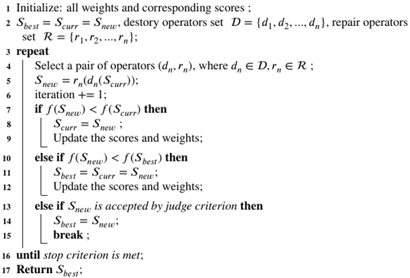
The main framework of the ALNS algorithm contains several parts, which are initial solution generation, neighborhood search, acceptance or rejection strategy of the solution, neighborhood update, and the algorithm termination conditions. The main steps are shown below, and the structure of ALNS is presented in Algorithm 1.
(1)
Initial solution generation: an initial solution is generated according to the characteristics of the problem. The initial solution can be generated in greedy approaches, random ways, and heuristic algorithms. Additionally, some parameters of the algorithm are initialized, such as the weights of the operators and the corresponding scores.
(2)
Neighborhood search operation: choose a set of destroy and repair operators; the solution is destroyed to obtain a new solution and subsequently a repair operation is conducted on it to obtain the current solution.
(3)
Acceptance or rejection strategy: the simulated annealing algorithm is generally used to control whether the current solution is accepted or not, followed by judging whether the termination condition is satisfied; if not, proceed to step (4).
(4)
Neighborhood update: the weights and scores of the operators are updated according to the quality of the current solution.
(5)
Algorithm termination conditions: algorithm termination conditions are generally set in terms of running time and a specified number of iterations.
Algorithm 1: The structure of the ALNS
Information 14 00331 i001
As shown in Algorithm 1, where S b e s t is used to represent the optimal solution, S c u r r represents the current solution, S n e w represents the new solution, D is used to represent the set of destroy operators, R is used to represent the set of repair operators, d n ( ) and r n ( ) denote the application of destroy and repair operators on the current solution, and f is the simulated annealing algorithm objective function.

4.1. Initial Solution Generation

Meta-heuristic algorithms generally need to generate an initial solution on which to iterate. Therefore, a good initial solution can speed up the solution search process and reduce the number of iterations of the algorithm. In this paper, the initial solution is constructed by greedy insertion. Specifically, all customer nodes are sorted according to the distance, the farthest one is selected as the endpoint, and an empty route containing the starting point and the endpoint is constructed using the central warehouse as the starting point. Subsequently, the closest customer nodes are added to the route in order without violating constraints such as vehicle capacity. The insertion process is repeated until no more customer nodes can be inserted to form the initial solution scheme.

4.2. Initial Solution Generation

The operators used in this algorithm are mainly revised from Demir et al. [33] and Ropke [27].
(1)
Random removal
This operator randomly selects a point t from the current solution and selects several client nodes i for deletion operations to be put into the list of deleted nodes M and the deleted client nodes n N .
(2)
Worst removal
This operator removes the customer node with the farthest distance from the current solution, assuming that the set of customer nodes is N = { 1 , 2 , , n } ; when the delivery vehicle travels from the previous node i to the current node j, there is a travel distance l i j , traverse all customer nodes, find the largest l i j , and add node j to the list of deleted nodes M .
(3)
Shaw removal
The operator was proposed by Shaw [28], and its key idea is to remove customer nodes with high similarity and evaluate the relevance of node i and node j by defining the relevance metric R i j . In this study, for the IDSMIPR, we use the distance l i j between customer nodes, the number of customer demands d i t , and the customer inventory capacity Q i to calculate the correlation R i j ; a smaller R i j represents a higher correlation between two customer nodes. Additionally, we use φ ,   ζ ,   λ to denote the weight of the influence of different factors on the correlation and have φ + ζ + λ = 1 . The specific correlation calculation formula is as follows:
R i j = φ ( l i j ) + ζ ( | d i d j | ) + λ ( | Q i Q j | )
(4)
Route removal
This operator randomly selects one of all routes for removal, randomly selects a client node i to remove it, and iteratively selects other nodes on the route to which the node belongs until all nodes are removed.
(5)
Neighborhood removal
This operator selects a node from the path that is most important for the average distance of that path to delete. Suppose there is the path set B and for each line B = { i 1 , i 2 , , i B } ; its average distance is calculated by d ¯ B = i 1 , i 2 B d i 1 i 2 / B . Select a node i * = a r g m a x B B ; j B { d ¯ B d B \ { i } } .
(6)
Demand-based removal
This operator is a special case of the Shaw operator. Let φ and λ be equal to zero and ζ be equal to 1 to compute the similarity between nodes and select nodes for deletion.
(7)
Greedy insertion
This operator selects a route to insert node i in the least-cost manner. Considering the specific objective function, the cost of inserting a node i in the IDSMIPR is given by Δ f i = l j i + l i k l j k , where i , j , k N .
(8)
Regret insertion
This operator was proposed by Potvin [34], mainly to solve the problem of placing the request with high insertion cost at the end of the Greedy insertion operator and this resulting in no position for insertion. By defining Δ f i 1 as the optimal insertion cost variation value and Δ f i 2 as the second best insertion cost variation value, then the node i * = a r g m a x i N Δ f i 2 Δ f i 1 is selected.
(9)
Random insertion
This operator randomly selects a node from the list of nodes M that have been removed and inserts it randomly into a route at some point in time and selects the node i * = a r g m i n i N Δ f i .
(10)
Sequential insertion
This operator sequentially selects a node from the list of deleted nodes M and inserts the node into the route according to the node selection of i * = a r g m i n i N Δ f i until no node can be inserted.
(11)
Swap insertion
The operator randomly selects two time periods and swaps the routes.

4.3. Operator Selection and Weight Adjustment

The adaptive selection method of the operator uses the roulette wheel method, which follows the rule that the more suitable the operator is, the higher the probability that he or she will be selected. The method assumes that the probability of an operator being selected is proportional to the performance of the operator, which can be described as follows. Suppose there are N operators and the weight score of each operator is w i > 0   ( i = 1 , 2 , , N ) . The probability that the ith individual is selected is given by the following formula: p i = w i i = 1 N w i . At the end of each iteration, the weight score of the operator needs to be updated, and the update formula is shown in (24) as follows:
w i s + 1 = ( 1 r ) w i s + r π i θ i
where θ i is the number of times the operator i was used during the previous iteration and r is the response factor that controls the speed of response of the operator weight adjustment process to changes in weight performance. If r = 0, then the weights remain constant; if r = 1, then the weights of the operators are determined by the most recent score [26].

4.4. Acceptance Criteria and Termination Conditions

This algorithm uses the Metropolis criterion of the simulated annealing algorithm to determine whether to accept the solution. The simulated annealing algorithm simulates the behavior of crystal molecules in the annealing process of solid substances to solve the optimization problem. It mainly generates an initial solution, sets the initial problem, and generates a new solution according to a certain strategy to determine whether the temperature of this solution reaches the target problem; if not, it continues to repeat the annealing process. The Metropolis criterion, on the other hand, is the basis of the simulated annealing algorithm, as shown in (25) by the following equation:
p t ( S c u r r = S n e w ) = 1 , E E e x p ( Δ E t ) , E > E
where E is the energy value in the annealing process, p t ( S c u r r = S n e w ) denotes the probability of accepting the new solution S n e w when E E or accepting the new solution when E > E . If e x p ( Δ E t ) is greater than a certain threshold, the new solution is accepted, otherwise the new solution is rejected.
There are two conditions for the termination of this algorithm, the first one is that the algorithm runs for the 1800s and the second one is that the number of iterations of the algorithm reaches 2000. As soon as the algorithm runs to one of the two conditions, the algorithm will stop running.

5. Case Study

In this section, simulated datasets of different sizes are used to validate the accuracy of the model and the effectiveness of the proposed ALNS algorithm. Among them, the small-size example contains 5, 10, and 15 customer points and the medium-size example contains 20, 25, and 30 customer points for numerical experimental analysis. The horizontal and vertical coordinates of these customer points are randomly generated in the range [0, 100], and the distances between customer points are expressed using Euclidean distances. The replenishment horizon of the customer is set to 3 days, and the demand of these customer points for the next 3 days is randomly generated according to the calculation criteria of the intermittent demand model. Moreover, the initial inventory of customers is randomly set to any integer value from 0 to the upper inventory limit. The units of measuring the capacity of the central warehouse, customers, and vehicles, as well as the demand, are the items. The inventory capacity of customers and other parameters used in the illustration are shown in Table 2. The experimental environment for this case study uses Python 3.9 programming, whereas the IDE environment is PyCharm 2022.1.2, the CPU is an Intel(R) Xeon(R) W-2255 CPU @ 3.70 GHz, and the memory is 64 GB.
Some of the operators used in the ALNS algorithm require the determination of several parameters, the values of which can have a large impact on the final algorithm’s solving power. Since the number of parameters is small, we use iterative trials to determine the optimal parameter values. The specific parameter values are shown in Table 3.
Subsequently, the ALNS algorithm is used to solve the above small-size and medium-size cases separately. Table 4 shows the algorithm distribution solution results for the small-size case with 10 customer points, and Table 5 presents the algorithm solution results for the medium-size case with 20 customer points.
The results of the experiment are shown in Table 4 and Table 5 for a replenishment cycle of 3 days. The second column shows the type of inventory replenishment and whether it was delivered by the warehouse or a lateral transshipment between stores. The third column shows the driving route of the vehicle, where the distribution cost and inventory cost are generated by the company’s own vehicle distributing from the warehouse, whereas transfer distribution provided by an external service provider generates the transfer cost. From the results in Table 4 and Table 5, it can be seen that the distribution cost accounts for a higher percentage of the total cost, whereas the inventory cost and the transfer cost account for a lower percentage. In general, products that need to be restocked have higher sales volumes. The first case is influenced by the region, where an item does not sell well in this store but sells well in other stores, thus creating a demand for transshipment. The second situation is that the item is not selling well in all stores; however, a store needs a certain amount of the product to avoid shortages.
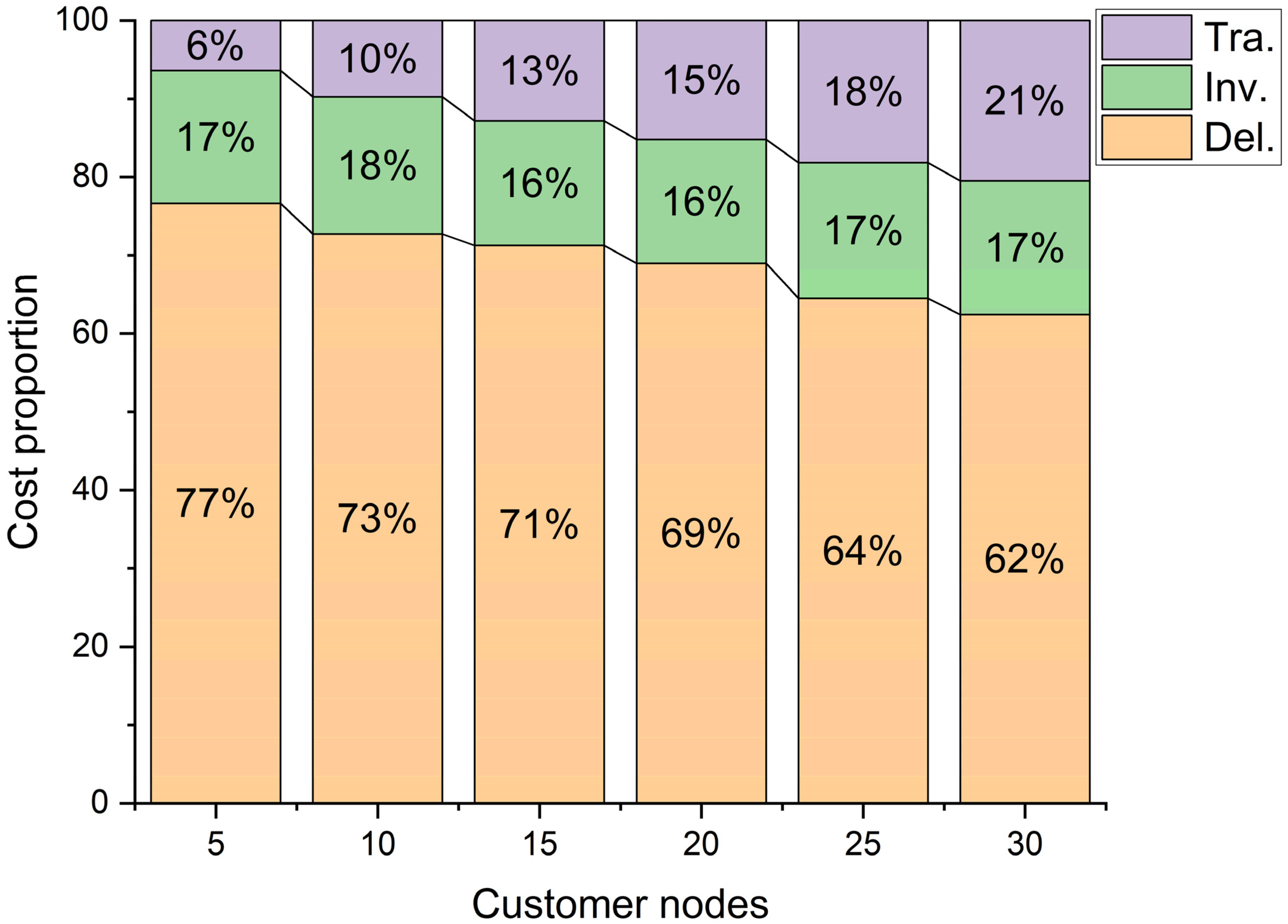
In addition, to understand the proportion of cost under different numbers of customer points, the proportion of distribution costs, inventory costs, and transshipment costs in the total cost is shown in Figure 2. From Figure 2, it can be seen that as the number of customer points increases, the proportion of distribution costs gradually decreases, the proportion of transshipment costs gradually increases, and the proportion of inventory costs shows a small increase. Therefore, with the increase in the number of customer points, the demand for transshipment will be elevated. In addition, an appropriate price for transshipment will help to reduce the distribution cost, balance the inventory of the region, and increase the profit of the company.
To observe the effect of vehicle capacity on the supply chain system, a sensitivity analysis was performed. We set the vehicle capacity to grow from 20 to 50 with an interval of 2 units to observe the change in the delivery cost. The number of customer nodes was set to 30. As shown in Figure 3, the distribution cost gradually decreases to a stable value. Thus, the increase in vehicle capacity can bring greater benefits. Larger vehicles are beneficial to reduce the remaining empty loading of vehicles and can merge more routes. When all node demands can be met by a large enough vehicle, only one vehicle is needed, making the cost of distribution stable.
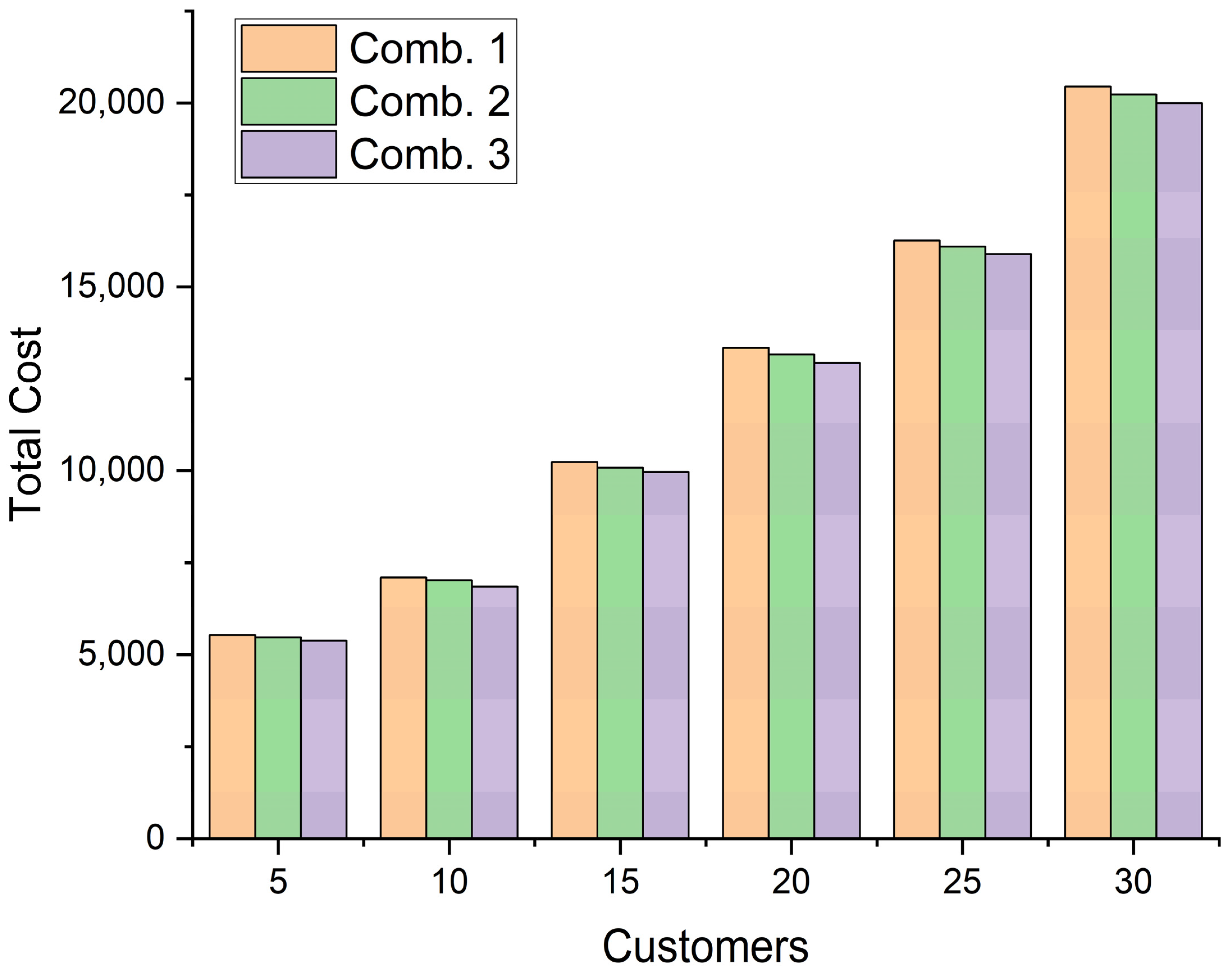
Operators have a large impact on the performance of the ALNS algorithm, and operators designed for different problems help to improve the search capability and achieve efficient solutions. Thus, we test the performance of the new operators by comparing the best solution. The method we use is to add the new operators into the ALNS algorithm one by one to observe the change in the optimal solution. In Figure 4, no new operator in “Comb. 1”, operator (3) is added in “Comb. 2”, operator (3) and operator (6) are added in “Comb. 3”. It is obvious that the addition of the new operator improves the quality of the optimal solution. “Comb. 2” and “Comb. 3” improved by an average of 1.19% and 2.80%, respectively.
We generate six cases at 5, 10, 15, 20, 25, and 30 customer points. Considering the randomness of the results, we used the Gurobi, TS, and ALNS algorithms to perform multiple solution tests and took the mean value of the results as the test results. The results of the algorithm comparison tests are shown in Table 6, where Z 1 , Z 2 , and Z 3 denote the objective function values solved by the Gurobi, TS, and ALNS algorithms, respectively, and T 1 , T 2 , and T 3 denote the solving time of the Gurobi, TS and ALNS algorithms, respectively. Gap1 denotes the percentage error of the solution results of the Gurobi and TS algorithms; Gap1 = 100 ×   ( Z 2 Z 1 ) / Z 1 . Gap2 denotes the percentage error of the solution results of the Gurobi and ALNS algorithms; Gap2 = 100 ×   ( Z 3 Z 1 ) / Z 1 .
From Table 6, we can find that the values of Gap1 and Gap2 are close to 0 for the cases with 5 and 10 customer points, which indicates that all three methods can find the optimal solution quickly when the number of customer points is small. In the cases with 15, 20, 25, and 30 customer points, the advantage of the TS algorithm gradually decreases compared with the commercial solver, and the value of Gap1 can reach a maximum of 2.59%. The advantage of the ALNS algorithm is gradually obvious, and the value of Gap2 can reach up to 1.77%. Due to the increase in the search neighborhood, the ALNS algorithm can obtain better solutions, whereas the TS algorithm may be trapped in the local optimal solution and cannot jump out.
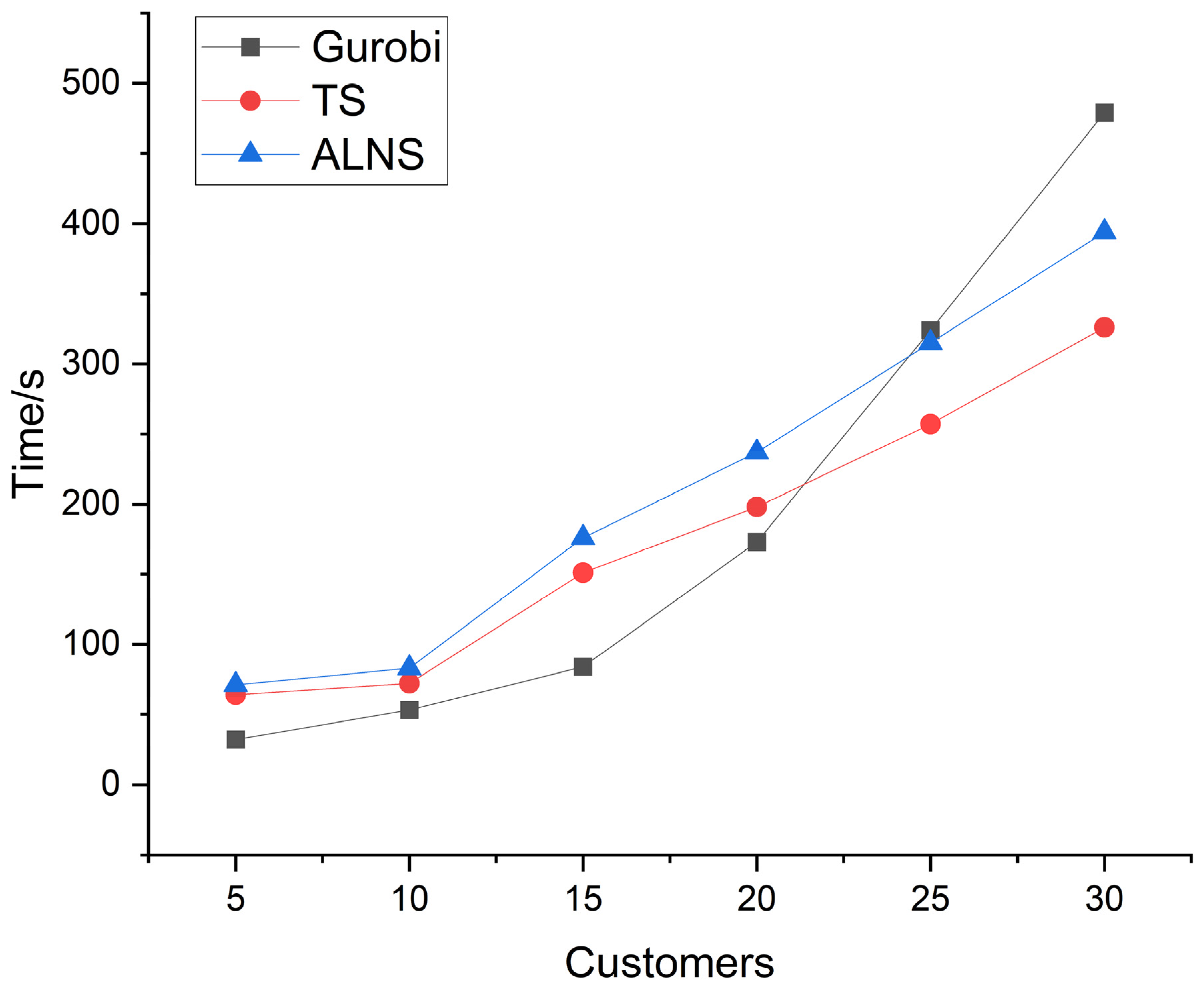
As shown in Figure 5, the running time of the Gurobi solver gradually increases with the increase in the case size and the increasing trend is higher than the other two algorithms. Compared with the TS algorithm, the solution time of the ALNS algorithm is slightly higher than that of the TS algorithm due to the increase in the searched neighborhood. Considering that the ALNS algorithm can obtain better quality solutions, the ALNS algorithm proposed in this study can effectively handle this class of the single-product multi-period IRP.
This study provides managerial insights to academia and industry. For academia, we focus on the IRP under intermittent demand, a particular demand pattern that can pose challenges for inventory management, creating inventory backlogs and raising inventory costs. To address this problem, we introduce a lateral transit strategy, build a two-stage model, and design an ALNS algorithm with new operators. Our study extends the scope of the IRP domain, and the proposed operators can improve the performance of the ALNS algorithm. For industry, the number of customers in a region has the greatest impact on the total cost of inventory management. At the same time, an increase in the number of nodes leads to more transshipment needs and reduces the distribution costs as a percentage of the total costs. Therefore, the implementation of a lateral transshipment strategy can effectively balance the regional inventory, lower the risk of demand shortage, and improve the efficiency of inventory management. In addition, the increase in distribution vehicle capacity can bring higher revenue. We offer the following suggestions to managers: (1) Use the lateral transshipment strategy to balance the inventory in the region. (2) Reduce transshipment prices and improve profits by finding external service providers, etc. (3) Determine the appropriate size of vehicle capacity according to the regional demand and use larger capacity models to reduce distribution costs.

6. Conclusions

This study considers the IRP in a two-echelon supply chain system consisting of a central warehouse and several customers. In this supply chain system, the intermittent demand pattern of products poses challenges for inventory management. On the one hand, the fluctuating demand of products can reduce the accuracy of replenishment planning. On the other hand, continuous backlogs of products can generate significant inventory holding costs and reduce the profitability of the system. In this context, we build a single-product multi-period inventory routing model with lateral transshipment. Before the replenishment planning period, the warehouse’s own vehicles are used to replenish products to customers. During the planning period, the lateral transshipment of products between customers is achieved using the distribution service provided by external service providers. An ALNS algorithm is also designed for solving the model.
The results show that the lateral transshipment strategy can provide a promising way to manage inventory for intermittent demand patterns and that transfer can effectively balance regional inventory, reduce distribution costs, and improve corporate profits. Specifically, distribution costs constitute the highest percentage of the total costs and the number of customer points has the greatest impact on distribution costs. Managers can increase the demand for transferring products between customer points to each other by lowering the price of transshipment and avoiding delivery from the central warehouse. In addition, an increase in vehicle capacity has a positive impact on reducing the distribution costs. In addition, our work extends the scope of the IRP and makes an academic contribution to solving IRP variants.
Several limitations of this study need to be acknowledged. On the one hand, we can consider multi-products in our future research. On the other hand, we can consider designing different transshipment strategies to match the actual business situation. Finally, more ALNS operators can be developed to improve the solving power of the algorithm.

Author Contributions

Conceptualization, X.S., T.L. and D.C.; methodology, X.S., T.L. and D.C.; software, X.S. and T.L.; validation, X.S.; formal analysis, X.S.; investigation, X.S.; resources, X.S.; writing—original draft preparation, X.S., T.L. and D.C.; supervision, D.C. All authors have read and agreed to the published version of the manuscript.

Funding

This research received no external funding.

Data Availability Statement

Not applicable.

Conflicts of Interest

The authors declare no conflict of interest.

Abbreviations

The following abbreviations are used in this study:
SymbolMeaning
Sets
N Set of all nodes, N = { 0 , 1 , 2 , , n }
A Set of all arcs, A = { ( i , j ) : i , j N , i j }
O Central warehouse, O = { 0 }
N Set of all customer nodes, N = N | { 0 }
T Set of periods, T = { 1 , 2 , 3 , , t }
K Set of vehicles, K = { 1 , 2 , 3 , , k }
Parameters
h 1 Unit inventory cost in the central warehouse
h 2 Unit inventory cost in customers
h 3 Delivery cost per unit distance
h 4 Transshipment cost per unit distance
Q i Inventory capacity of customers, i N
C Capacity of vehicles
l i j Distance between node I and j
Variables
d i t The actual demand of node i at period t,  i N , t T
x i j k t At period t, the vehicle k visits node j after visiting node i, i , j N , i j , k K , t T
r i j t The number of goods transferred from node i to node j at period t, i , j N , i j , t T
I i t The inventory level of node i at the beginning of period t, i N , t T
q i k t The number of goods transported by vehicle k from the central warehouse to node i at time t, i N , k K , t T
v i k t Dummy variables for sub-loop elimination

References

  1. Biuki, M.; Kazemi, A.; Alinezhad, A. An integrated location-routing-inventory model for sustainable design of a perishable products supply chain network. J. Clean. Prod. 2020, 260, 120842. [Google Scholar] [CrossRef]
  2. Dey, B.K.; Seok, H. Intelligent inventory management with autonomation and service strategy. J. Intell. Manuf. 2022, 1–24. [Google Scholar] [CrossRef]
  3. Mandal, B.; Dey, B.K.; Khanra, S.; Sarkar, B. Advance sustainable inventory management through advertisement and trade-credit policy. RAIRO-Oper. Res. 2021, 55, 261–284. [Google Scholar] [CrossRef]
  4. Dalalah, D.; Al-Araidah, O. Dynamic decentralised balancing of CONWIP production systems. Int. J. Prod. Res. 2010, 48, 3925–3941. [Google Scholar] [CrossRef]
  5. Wu, S.N.; Liu, Q.; Zhang, R.Q. The Reference Effects on a Retailer’s Dynamic Pricing and Inventory Strategies with Strategic Consumers. Oper. Res. 2015, 63, 1320–1335. [Google Scholar] [CrossRef]
  6. Williams, T.M. Stock Control with Sporadic and Slow-Moving Demand. J. Oper. Res. Soc. 1984, 35, 939–948. [Google Scholar] [CrossRef]
  7. Syntetos, A.A.; Boylan, J.E.; Croston, J.D. On the categorization of demand patterns. J. Oper. Res. Soc. 2005, 56, 495–503. [Google Scholar] [CrossRef]
  8. Turkmen, A.; Januschowski, T.; Wang, Y.Y.; Cemgil, A. Intermittent Demand Forecasting with Renewal Processes. arXiv 2010, arXiv:2010.01550. [Google Scholar]
  9. Wu, W.T.; Zhou, W.; Lin, Y.; Xie, Y.Q.; Jin, W.Z. A hybrid metaheuristic algorithm for location inventory routing problem with time windows and fuel consumption. Expert Syst. Appl. 2021, 166, 114034. [Google Scholar] [CrossRef]
  10. Olgun, M.O.; Aydemir, E. A new cooperative depot sharing approach for inventory routing problem. Ann. Oper. Res. 2023, 307, 417–441. [Google Scholar] [CrossRef]
  11. Dantzig, G.B.; Ramser, J.H. The Truck Dispatching Problem. Manag. Sci. 1959, 6, 80–91. [Google Scholar] [CrossRef]
  12. Alkaabneh, F.; Diabat, A. A multi-objective home healthcare delivery model and its solution using a branch-and-price algorithm and a two-stage meta-heuristic algorithm. Transp. Res. Part C Emerg. Technol. 2023, 147, 103838. [Google Scholar] [CrossRef]
  13. Mousavi, R.; Salehi-Amiri, A.; Zahedi, A.; Hajiaghaei-Keshteli, M. Designing a supply chain network for blood decomposition by utilizing social and environmental factor. Comput. Ind. Eng. 2021, 160, 107501. [Google Scholar] [CrossRef]
  14. Yin, Y.; Liu, X.; Chu, F.; Wang, D. An exact algorithm for the home health care routing and scheduling with electric vehicles and synergistic-transport mode. Ann. Oper. Res. 2023, 1–36. [Google Scholar] [CrossRef]
  15. Bell, W.J.; Dalberto, L.M.; Fisher, M.L.; Greenfield, A.J.; Jaikumar, R.; Kedia, P.; Mack, R.G.; Prutzman, P.J. Improving the Distribution of Industrial Gases with an On-Line Computerized Routing and Scheduling Optimizer. Interfaces 1983, 13, 4–23. [Google Scholar] [CrossRef]
  16. Abdelmaguid, T.F.; Dessouky, M.M.; Ordóñez, F. Heuristic approaches for the inventory-routing problem with backlogging. Comput. Ind. Eng. 2009, 56, 1519–1534. [Google Scholar] [CrossRef]
  17. Raa, B.; Aghezzaf, E.-H. A practical solution approach for the cyclic inventory routing problem. Eur. J. Oper. Res. 2009, 192, 429–441. [Google Scholar] [CrossRef]
  18. Geiger, M.J.; Sevaux, M. On the Use of Reference Points for the Biobjective Inventory Routing Problem. arXiv 2011, arXiv:1109.3094. [Google Scholar]
  19. Cárdenas-Barrón, L.; González-Velarde, J.L.; Treviño-Garza, G.; Garza-Nuñez, D. Heuristic algorithm based on reduce and optimize approach for a selective and periodic inventory routing problem in a waste vegetable oil collection environment. Int. J. Prod. Econ. 2019, 211, 44–59. [Google Scholar] [CrossRef]
  20. Lefever, W.; Aghezzaf, E.; Hadj-Hamou, K.; Penz, B. Analysis of an improved branch-and-cut formulation for the Inventory-Routing Problem with Transshipment. Comput. Oper. Res. 2018, 98, 137–148. [Google Scholar] [CrossRef]
  21. Coelho, L.C.; Maio, A.D.; Laganà, D. A variable MIP neighborhood descent for the multi-attribute inventory routing problem. Transp. Res. Part E Logist. Transp. Rev. 2020, 144, 102137. [Google Scholar] [CrossRef]
  22. Rayat, F.; Musavi, M.; Bozorgi-Amiri, A. Bi-objective reliable location-inventory-routing problem with partial backordering under disruption risks: A modified AMOSA approach. Appl. Soft Comput. 2017, 59, 622–643. [Google Scholar] [CrossRef]
  23. Soysal, M.; Bloemhof-Ruwaard, J.; Haijema, R.; Vorst, J.G.V.D. Modeling a green inventory routing problem for perishable products with horizontal collaboration. Comput. Oper. Res. 2018, 89, 168–182. [Google Scholar] [CrossRef]
  24. Ji, Y.; Du, J.H.; Han, X.Y.; Wu, X.Q.; Huang, R.P.; Wang, S.L.; Liu, Z.M. A mixed integer robust programming model for two-echelon inventory routing problem of perishable products. Physica A 2020, 548, 124481. [Google Scholar] [CrossRef]
  25. Achamrah, F.E.; Riane, F.; Limbourg, S. Spare parts inventory routing problem with transshipment and substitutions under stochastic demands. Appl. Math. Model. 2022, 101, 309–331. [Google Scholar] [CrossRef]
  26. Ortega, E.; Doerner, K. A sampling-based matheuristic for the continuous-time stochastic inventory routing problem with time-windows. Comput. Oper. Res. 2023, 152, 106129. [Google Scholar] [CrossRef]
  27. Ropke, S.; Pisinger, D. An Adaptive Large Neighborhood Search Heuristic for the Pickup and Delivery Problem with Time Windows. Transp. Sci. 2006, 40, 455–472. [Google Scholar] [CrossRef] [Green Version]
  28. Shaw, P. Using Constraint Programming and Local Search Methods to Solve Vehicle Routing Problems. In Proceedings of the Principles and Practice of Constraint Programming—CP98: 4th International Conference, CP98, Pisa, Italy, 26–30 October 1998. [Google Scholar]
  29. Coelho, L.C.; Cordeau, J.-F.; Laporte, G. Consistency in multi-vehicle inventory-routing. Transp. Res. Part C Emerg. Technol. 2012, 24, 270–287. [Google Scholar] [CrossRef]
  30. Coelho, L.C.; Cordeau, J.-F.; Laporte, G. The inventory-routing problem with transshipment. Comput. Oper. Res. 2012, 39, 2537–2548. [Google Scholar] [CrossRef]
  31. Adulyasak, Y.; Cordeau, J.-F.; Jans, R. Optimization-Based Adaptive Large Neighborhood Search for the Production Routing Problem. Transp. Sci. 2014, 48, 20–45. [Google Scholar] [CrossRef]
  32. Alkaabneh, F.; Shehadeh, K.S.; Diabat, A. Routing and resource allocation in non-profit settings with equity and efficiency measures under demand uncertainty. Transp. Res. Part C Emerg. Technol. 2023, 149, 104023. [Google Scholar] [CrossRef]
  33. Demir, E.; Bektaş, T.; Laporte, G. An adaptive large neighborhood search heuristic for the Pollution-Routing Problem. Eur. J. Oper. Res. 2012, 223, 346–359. [Google Scholar] [CrossRef]
  34. Potvin, J.-Y.; Rousseau, J.-M. A parallel route building algorithm for the vehicle routing and scheduling problem with time windows. Eur. J. Oper. Res. 1993, 66, 331–340. [Google Scholar] [CrossRef]
Figure 1. Example of a lateral transshipment inventory routing model.
Information 14 00331 g001
Figure 2. Inventory routing cost proportion chart.
Information 14 00331 g002
Figure 3. Vehicle capacity cost analysis.
Information 14 00331 g003
Figure 4. Operator performance comparison.
Information 14 00331 g004
Figure 5. Comparison of solution times.
Information 14 00331 g005
Table 1. Key literature on the IRP.
ReferencePeriod TypeDemand TypeCommodity TypeFleet CompositionSolution Method
Cárdenas-Barrón et al. [19]MultipleDeterministicSingleHomogeneousHeuristics
Lefever et al. [20]MultipleDeterministicSingleHomogeneousExact
Coelho et al. [21]MultipleDeterministicMultipleHeterogeneousExact
Rayat et al. [22]MultipleStochasticMultipleHeterogeneousMetaheuristics
Soysal et al. [23]MultipleStochasticMultipleHomogeneousCPLEX
Ji et al. [24]SingleStochasticSingleHomogeneousGurobi
Achamrah et al. [25]MultipleStochasticMultipleHomogeneousApproximation
Ortega and Doerner [26]MultipleFuzzyMultipleHomogeneousMetaheuristics
This workMultipleIntermittentMultipleHomogeneousMetaheuristics
Table 2. The parameter values of the model.
ParameterDescriptionValueUnit
ONumber of central warehouses1-
PNumber of products1-
N Number of customer nodes5, 10, 15, 20, 25, 30-
a i , b i Customer point coordinates([0, 100], [0, 100])-
l i j Customer distance ( a i a j ) 2 + ( b i b j ) 2 km
T Periods3day
K Number of vehicles[1, 10]-
h 1 Unit inventory cost in the central warehouse2dollar
h 2 Unit inventory cost in customers4dollar
h 3 Delivery cost per unit distance5dollar
h 4 Transshipment cost per unit distance3dollar
CCapacity of vehicles30item
Q i Capacity of customers, i N [3, 8]item
Table 3. The parameter value of ALNS.
ParameterValueDescription
φ 0.7Shaw removal operator, distance correlation weights between client nodes
ζ 0.2Shaw removal operator, customer demand quantity relevance weights
λ 0.1Shaw removal operator, customer inventory capacity correlation weights
r 0.8Response factors in roulette strategy
Table 4. Small-size calculation distribution results.
TypeRouteDelivery CostsInventory CostsTransshipment CostsTotal CostTime/s
Day oneDelivery0-2-8-1-6-01375396---
Transshipment3-5-4--318--
Day twoDelivery0-7-9-4-10-01140492---
Transshipment6-8--129--
Day threeDelivery0-8-4-7-9-2-01810312---
Transshipment5-3-1--222--
Total 43251200669619483
Table 5. Medium-size calculation distribution results.
TypeRouteDelivery CostsInventory CostsTransshipment CostsTotal CostTime/s
Day oneDelivery0-1-9-11-15-14-17-0,
0-12-2-8-5-4-0,
0-19-3-6-7-0
3635632---
Transshipment13-10-16--645--
Day twoDelivery0-8-2-9-7-16-0,
0-3-5-12-14-0,
0-11-17-19-1-2-0
2815686---
Transshipment6-4-15--771--
Day threeDelivery0-13-2-18-11-12-3-0,
0-7-1-15-19-0,
0-4-16-17-5-0
2465728---
Transshipment2-6-20--552--
Total 89152046196812,929237
Table 6. Comparison of algorithm test results.
NodesGurobiTSALNSError
Z 1 T 1 Z 2 T 2 Z 3 T 3 Gap1Gap2
55381325387645385710.000.00
106828536859726850830.46%0.32%
15990284999715199671760.96%0.66%
2012,81217313,00119812,9292371.48%0.91%
2515,68232416,02925715,8903152.21%1.33%
3019,64847920,15732619,9963942.59%1.77%
Disclaimer/Publisher’s Note: The statements, opinions and data contained in all publications are solely those of the individual author(s) and contributor(s) and not of MDPI and/or the editor(s). MDPI and/or the editor(s) disclaim responsibility for any injury to people or property resulting from any ideas, methods, instructions or products referred to in the content.