Abstract
Industrial radiography is a pivotal non-destructive testing (NDT) method that ensures quality and safety in a wide range of industrial sectors. Conventional human-based approaches, however, are prone to challenges in defect detection accuracy and efficiency, primarily due to the high inspection demand from manufacturing industries with high production throughput. To solve this challenge, numerous computer-based alternatives have been developed, including Automated Defect Recognition (ADR) using deep learning algorithms. At the core of training, these algorithms demand large volumes of data that should be representative of real-world cases. However, the availability of digital X-ray radiography data for open research is limited by non-disclosure contractual terms in the industry. This study presents a pipeline that is capable of modeling synthetic images based on statistical information acquired from X-ray intensity distribution from real digital X-ray radiography images. Through meticulous analysis of the intensity distribution in digital X-ray images, the unique statistical patterns associated with the exposure conditions used during image acquisition, type of component, thickness variations, beam divergence, anode heel effect, etc., are extracted. The realized synthetic images were utilized to train deep learning models, yielding an impressive model performance with a mean intersection over union (IoU) of 0.93 and a mean dice coefficient of 0.96 on real unseen digital X-ray radiography images. This methodology is scalable and adaptable, making it suitable for diverse industrial applications.
1. Introduction
Non-destructive Testing (NDT) plays a pivotal role in maintaining the safety and reliability of diverse structural components across multiple industries. This is achieved in a manner that ensures inspected components are not damaged or impaired in terms of their intended functionality. In safety-critical sectors like aerospace [1] and automotive [2] sectors, NDT is crucial for identifying potential failures and defects and mitigating the potential dangers that could arise from the failure of such components during service. Over the years, diverse NDT methods have been developed and employed in the industry. These methods include but are not limited to visual inspection, magnetic particle inspection, liquid penetrant inspection, ultrasonic inspection, infrared thermography, X-ray radiography, etc. However, X-ray radiography stands out due to its ability to provide details of the internal structures of components, enabling the visualization of flaws such as cracks, voids, inclusions, shrinkage cavities, etc. [3], within inspected components, offering a unique perspective that is unattainable using surface inspection methods. Digital X-ray radiography presents a fascinating blend of simplicity and complexity, where its simplicity lies in its basic operation: generated X-ray photons pass through an object under test and are captured using a detector, producing a two-dimensional (2D) image [4]. Generated digital X-ray radiography images are typically rendered in shades of gray, having gray values ranging from 0 to 65535 for 16-bit images or 0 to 255 gray values for 8-bit images. The principal factor influencing the noticeable gray value difference within acquired radiographic images is X-ray beam attenuation [5], which is affected by factors such as differences in material thickness, density, foreign material inclusions, and the geometry of the components being inspected, among others [6]. The seemingly simple process of X-ray image acquisition conceals the intricate physics and engineering that underpin the technique. The processes of X-ray generation, exposure controls and effect on image quality, acquisition setup, type of detectors that accurately capture X-ray photons (scintillation-based or direct X-ray conversion digital detector arrays), conversion of detected signals to digital signals, digital processing, etc., are all governed by very complex scientific principles [7]. Furthermore, collapsing a three-dimensional (3D) test component into a 2D representation presents a notable complexity and challenge with X-ray radiography because it can lead to the superimposition of features such as porosities, shrinkage cavities, cold fills, and foreign inclusions, which may occur at different depths within test components. As a result, the interpretation of acquired images becomes more difficult and prone to misconceptions, hence necessitating the services of trained experts for interpretation [8].
The challenges in interpreting digital X-ray images are additionally heightened by the nuance of some defects, which may not be prominent, especially in low-contrast radiographic images. According to ASTM 1316-17a [9], inspectors are typically tasked with accurately identifying radiographic indications, determining their relevance (flaws or not), evaluating if detected flaws constitute a defect, and reaching a decision on whether a component is to be accepted for use or rejected. Despite the post-processing assistance obtainable using computer-based operations, interpretations by experts are prone to human error, especially in the face of the high inspection demand occasioned by the high production throughput witnessed in manufacturing industries. This is especially evident in the aluminum die-casting industry, where process automation facilitates high manufacturing throughput [10].
1.1. Deep Learning in Digital X-ray Radiography Applications
The advent of deep learning, a subset of machine learning marked by algorithms that can interpret and learn from data, has revolutionized industrial inspection. Tasks involving feature recognition and image interpretation have witnessed the integration of such machine learning-based solutions across different industrial sectors [11]. Expanding beyond these, there are other industrial inspection solutions based on machine learning solutions, such as anomaly detection in environmental sensor networks [12] and online fault detection and classification in photovoltaic plants [13]. In non-destructive testing, deep learning models have achieved remarkable success in flaw/defect detection tasks in digital X-ray radiography applications [14]. Deep learning models, trained on extensive datasets of annotated images, show a convincing ability to detect patterns and anomalies, even those that are often difficult for the human eye. This cognitive capability of the algorithms is especially promising in NDT digital X-ray radiography, recording successes as highlighted by [15]. Hence, utilizing algorithms trained on large collections of digital X-ray images proffers a means of automating the defect detection process. This automation has the potential to improve the accuracy and efficiency of inspections and reduce human error [16]. Furthermore, automating image interpretation could boost the inspection throughput to meet the rising demands witnessed in manufacturing industries and ultimately lead to safer and more reliable outcomes. However, the application of deep learning in digital X-ray radiography is not without its challenges. A primary challenge is the lack of large volumes of annotated datasets of digital X-ray images that are representative of the use case intended. Owing to the sensitive nature of X-ray images, especially in safety-critical industries like aerospace and automotive, stringent non-disclosure confidentiality agreements are often reached between clients and the industry, which inadvertently limit the availability of X-ray images for open research [17,18].
Without sufficient representative data for a given use case, the potential of deep learning in enhancing automated defect detection in X-ray radiography would remain largely untapped [8]. To ameliorate the notable scarcity of large volumes of annotated datasets, synthetic data generation using computational models has sufficed as a viable solution, offering a promising pathway to realizing a vast number of training data that closely mimic real-world conditions [14,19]. This approach can utilize simulations of the X-ray imaging process, incorporating different materials, defect types, and geometries in a bid to produce diverse and realistic datasets. However, the question remains: how effective is such an approach?
1.2. X-ray Radiography Simulation
X-ray radiography simulators have proven to be very useful in NDT radiography due to the enormous values it brings, including enhancing NDT techniques, training experts, improving reliability and capability of testing approaches, inspection planning to efficiently analyze complex geometries, etc. [20]. The simulators play a crucial role in shortening the development time of new NDT techniques, especially in industries like aerospace, where structural integrity is very critical. The simulators are developed with varying complexities, from ray-tracing-based simulators to Monte Carlo-based simulators [21,22]. At the core of the functionality of these simulators is an in-depth focus on the modeling of X-ray generation and photon-matter interaction. The seeming realism that X-ray simulator images present has spurred several research interests, especially within deep learning applications, to leverage such synthetic data to address the shortage of real X-ray radiography datasets for training deep learning algorithms. This approach of using synthetic data as a data augmentation strategy is not new, as there have been published successes in the literature, covering applications not limited to autonomous vehicle development [23], facial recognition technology [24], and even NDT digital X-ray radiography, which this study is focused on. The primary objective of this research approach is for the model, trained on synthetic data, to yield high performance in actual real-case scenarios. Therefore, the need to have real-like synthetic data becomes critical, attracting notable research efforts aimed at generating same. Studies conducted by [25], they took a data synthetization approach that employs various image translation operations such as translation, rotation, zooming, shearing, etc. However, because the original data were real X-ray radiography images, certain operations such as shearing of the images, could significantly alter the essential image parameters of the resultant images, potentially making them less useful in training. In other studies, refs. [26,27] adopted the use of Monte Carlo simulation, which, in contrast to our proposed approach, comes at an additional computational cost. Additionally, their work adopts Lambert-beer’s equation to determine the primary intensity of the generated synthetic images, assuming monochromatic energy source. Although gaussian noise addition at different levels was introduced, the primary intensity generation does not offer the realism that is obtainable with polychromatic X-ray sources, which are mostly used in industry. In another research by [28], they explored training a deep learning algorithm using synthetic data, then fine-tuning the same on a real X-ray image data. The fine-tuned model was then employed for defect detection and classification.
In contrast to the considered literature, our approach takes a distinctive stance by modeling synthetic images using statistical distribution of intensity values from real X-ray radiography images to enhance overall model performance. This is achieved via a computationally less expensive solution, in contrast to, for instance, ray-casting or Monte Carlo simulations considered in the reviewed literature. Additionally, the gray value distribution from the real images is characteristic of the exposure conditions used to acquire such images. Furthermore, this study employs only synthetically generated data for training the model to be tested on real digital X-ray radiography images.
2. Intensity Distribution: Real vs. Simulated Images
A radiography image is a 2D matrix of pixel intensities, which represents the X-ray photons detected using a sensor during acquisition. Each pixel in this matrix corresponds to a specific finite area on the detector, and its value corresponds to the intensity of the photons detected at that specific area during image acquisition. When a test component is positioned between the source and the detector, the detected signal, converted to pixel intensity, is primarily indicative of the interactions that the X-ray photons have undergone while transmitting through the test component. Higher pixel intensity implies more photons were detected, which usually corresponds to areas in the test component that absorbed fewer X-ray photons (like porosities or shrinkage cavities), while lower intensity indicates fewer X-ray photons were detected, typically in areas where more X-rays were attenuated (like regions with higher material thickness) [29]. In principle, the X-ray beam originates from a small focal spot in the X-ray tube and assumes a divergent orientation as it travels toward the detector. This beam divergence, or spread, makes it possible to attain beam coverage over a wider 2D area of the detector [29]. Therefore, this divergence affects the photon intensity detected by the sensor, where the highest intensities are recorded at the central beam position, as this area receives the most direct and concentrated beam of X-ray photons. If this position is at the center of the detector, an observation across the entire detector should reveal a decrease in detected X-ray photon intensity that spans radially away from the center of the detector towards its edges. This decrease in intensity is attributed to the photons being more spread out and less concentrated towards the sides of the detector [30].
Another phenomenon that further influences the distribution of photon intensity across radiographic images is the anode heel effect [31]. In most X-ray tubes, the anode (the component that emits X-rays) is positioned at an angle, leading to the generation of X-ray beam intensity distribution that is not uniform when the X-ray photons are sensed by the detector. This is because the angled anode partially absorbs some of the X-rays on its side, resulting in a reduction in intensity towards the anode side of the beam. In addition, the interaction of X-ray photons with a component could lead to scatter radiation, which also influences intensity distribution in radiographic images [32]. This scattered radiation can reach the detector and contribute to image formation, but it does not carry useful information about the test component’s internal structure. Instead, it adds a level of noise to the image, which can reduce image quality. Scatter radiation is more significant in thicker and denser objects [33]. All the above image intensity altering factors discussed assume a uniform detector response across all the pixels of a detector. Hence, it is possible to theoretically model and implement the physics of X-ray imaging in such an ideal manner. However, there are a lot of other factors that influence intensity distribution, as seen on acquired X-ray radiography images.
2.1. Pixel Based Contributions
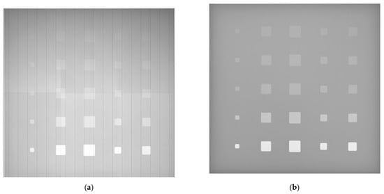
The response of these pixels may vary, even at the same level of X-ray photon exposure. Furthermore, with continuous use of the detector, there is an increasing possibility of degradation of the pixel performance across the detector over time [34]. Common pixel-based defects of the X-ray detectors include noisy pixels, over-responding pixels, under-responding pixels, dead pixels, non-uniform pixels, lag pixels, and bad neighborhood pixels. Depending on the type of pixel defect, a single pixel or a cluster of pixels could be affected. Detailed information on these mentioned pixel defects is offered in ASTM E2597 Standard Practice for Manufacturing Characterization of Digital Detector Arrays [35]. Ideal practices employ correction for defective pixels via interpolation of neighboring pixels. In addition, further processing of the acquired image is necessary, which includes averaging of different raw images, flat fielding of the images to correct the anode heel effect and uneven detector panel response [30], application of lookup tables (where necessary) [31], etc. Figure 1 shows an example of raw intensity distribution detected using the digital detector array and the outcome after necessary pixel intensity correction processes have been performed. Considering that the mentioned steps are unique to specific X-ray imaging systems, it becomes daunting to obtain a single simulation solution that will be robust enough to fully mimic all acquisition environments and image outputs.
2.2. Bridging the Research Gap
This research aims to develop a pipeline for generating synthetic digital X-ray images and utilizing these images to train a deep learning algorithm for the detection and segmentation of flaws in NDT digital X-ray radiography. Our approach has the potential not only to overcome the limitations posed by the scarcity of datasets but also to revolutionize the way training data is curated, consequently enhancing flaw detection models. In effect, the results offered by this study should influence the development of solutions that could enhance the safety and reliability of various industrial components.
3. Materials and Methods
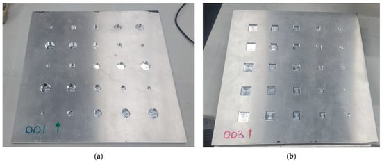
In our research, we employed aluminum plates for data collection purposes, each plate measuring 300 mm × 300 mm × 6.5 mm. Distributed across each of the six plates used in this study are 25 flat-bottom holes, resulting in a total of 150 flat-bottom holes. These holes were drilled using an end milling machining procedure and varied in shape, being either cylindrical or cuboidal. The cylindrical holes had a diameter ranging from 9 mm to 20 mm, while the cuboidal holes had side dimensions ranging from 7 mm to 20 mm. The depth of the holes also varied from a minimum depth of 0.5 mm, with 0.5 mm incremental steps, to a maximum depth of 5.5 mm. Figure 2 shows examples of the plates used in the study. By varying the depth of these flat bottom holes, the dataset captures a wide range of potential defect presentations that are of interest in this study. This variability is crucial for training a model capable of generalizing over a broad range of defect representations in real X-ray images to be later considered.
Furthermore, we utilized a digital X-ray radiography acquisition system with a maximum tube voltage of 150 kV and a maximum tube current of 0.5 mA. The system included a scintillation-based 2D digital detector array (DDA) with an active detection area of pixels (9,594,506 pixels) and a pixel size of 100 microns. Throughout the imaging of the aluminum plates, we consistently used a Source-to-Detector Distance (SDD) of 600 mm, with each plate placed directly on the detector during acquisition. The idea of using a consistent setup was to ensure similar gray value distribution across all plates for a given exposure factor, particularly in areas of equal thickness. Due to the expansive size of the DDA, the entire size of an aluminum plate (as considered in this study) could be captured in a single acquisition. However, it is important to note that the diverging nature of the X-ray beam from the tube’s focal spot to the detector results in an inhomogeneous distribution of X-ray intensity across the detector. Reasons for this inhomogeneity include the inverse relationship of the radiation intensity to the square of the beam’s travel distance from the source [36]. Additionally, the anode heel effect earlier discussed contributes to the inhomogeneity in gray value (GV) distribution. Therefore, by implication, the gray value distribution we observed differed across the plate, even at regions with the same thickness. Table 1 provides the exposure factors utilized for each plate. Varying the exposure factors significantly varied the intensity distribution across each acquisition, altering the image quality parameters such as the Signal-to-Noise ratio and Contrast-to-Noise ratio values across the defective areas (flat-bottom holes) and non-defective regions of the plates [37].
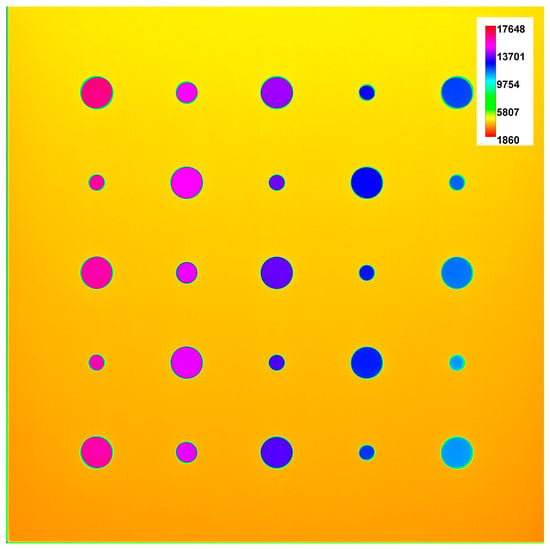
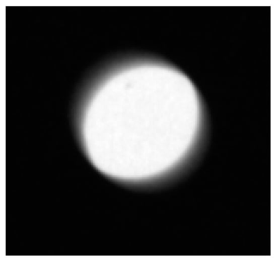
Flat-bottom holes with different depths relative to the plate’s thickness show distinct features representing higher signal intensity at their respective regions, demonstrating the effect of differential X-ray beam attenuation. This can be seen in Figure 3. Given the planner nature of the plate, the rendering of the 3D features (actual holes on the plate) on 2D X-ray images acquired using transmission X-ray radiography are described as follows: the cylindrical holes appear as circular features, while the cuboidal flat-bottom holes appear as square shaped features. This is particularly true when the central X-ray beam is parallel and at the central axis of the holes. However, due to the divergent nature of the X-ray beam, as discussed earlier, the resultant morphology of the rendered features is influenced by two factors: the depth of the flat-bottom holes and their proximity to the central X-ray beam path. Holes with more depth and positioned farther away from the central beam tend to increase the deviation from the ideal morphology (circle or square). Additionally, the edges are blurred due to effects such as X-ray beam scattering [38], the finite size of the focal spot, and the geometry of the setup [39]. Figure 4 offers an example of these effects.
Figure 3.
A color-spectrum representation of an acquired grayscale X-ray radiography image, showing inhomogeneous intensity distribution across the same thickness regions of the plate.
Figure 4.
A cropped X-ray radiography image showing the edge effect due to the geometry of the cylindrical flat-bottom hole and the X-ray beam divergence.
Due to the inhomogeneity witnessed in the acquired images, it was important to consider regions on each image that are statistically different. Hence, a total of 3000 cropped images were realized: 25 × 20 × 6 (features per plate × number of exposures × number of plates) to have a robust representation during synthetic image generation. However, it was important to identify and isolate images with saturated pixels, where 698 implicated images were isolated from the dataset, leaving a total of 2311 candidate real cropped digital X-ray images (1411 circular features and 900 with square features).
3.1. Synthetic Image Generation
The generation of synthetic digital X-ray images forms the cornerstone of this research, offering a viable approach to bridging the gap in the availability of data for training deep learning models in NDT digital X-ray radiography applications. The first step in this process involves a comprehensive analysis of real X-ray radiography images. This analysis focused on understanding the statistical distribution of gray values within real digital X-ray images considered. The intensity distribution of the 1411 digital X-ray images with circular flaws was analyzed. Statistical measures were obtained of the gray values at the background and at the features that represent areas with different plate thicknesses because of the presence of flat-bottom holes. These statistical measures included the following: Minimum GV, Maximum GV, Mean GV, Standard Deviation of GV, and Variance. The background had a defined Region of Interest (ROI) for all the images. The ROI for each feature within an image was determined using the maximum inscribed polygons within the edges of annotated features in the ground truth masks. To obtain a statistical representation of the actual remaining thickness of the plate, it was crucial to reduce the size of the inscribed polygons by 6 pixels, considering the effect described in Figure 4.
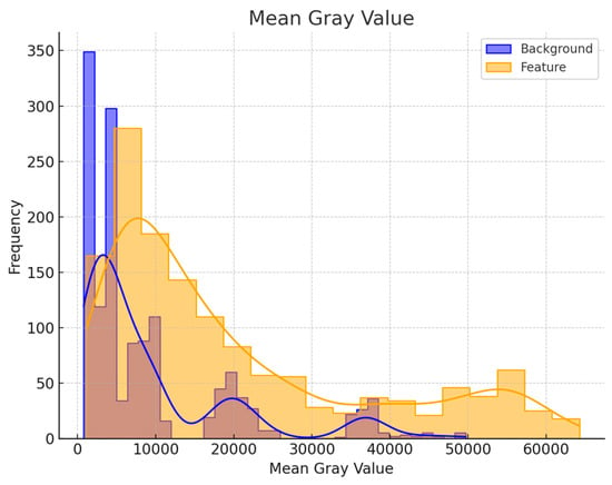
Figure 5 shows a superimposed histogram plot of the mean gray values of the assessed 1411 real X-ray images with circular features measured at the regions of the features and backgrounds. The distribution of the measured values stems primarily from the different exposure conditions used and the varying thicknesses of the flat-bottom holes in the imaged plates. Additionally, the inhomogeneity of the X-ray intensity further influences the distribution of these measured values.
Figure 5.
Superimposed histogram representation of the mean gray values measured in the considered 1411 real X-ray radiography images with circular features. The blue and orange lines represent the smoothed distribution of data for background and features respectively.
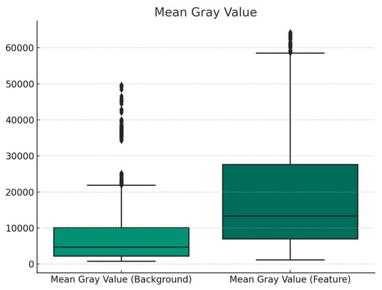
The box-and-whiskers plot in Figure 6. offers a unique presentation of the assessed data that is relevant in understanding how robust, or not, our data is in terms of feature representation. It could be observed that the interquartile ranges of the mean GV of the features, which represent 50% of our data, lie around 7000 to 28,000 GV. The upper whisker, which ranges between the 3rd quartile and the maximum (representing 25% of the data), has values ranging from 28,000 to around 58,000 gray values. Outliers could be observed above the 58,000 gray values. Depending on the expectations in a real scenario, this distribution could be used strategically to build the dataset.
Figure 6.
Box-and-whiskers plot of the mean gray values measured in the considered 1411 real X-ray radiography images with circular features.
The variations in gray value distribution are indicative of various material thicknesses (normal plate thickness and plate thickness at regions with flaws). With the statistical data extracted from the 1411 real digital X-ray images with circular features, we employed a specialized algorithm to generate synthetic images. This algorithm randomly generates gray values for the synthetic images but within the confines of the statistical distribution that was sampled in the real digital X-ray images. This approach ensures that the synthetic images, while randomly generated, still adhere to realistic patterns witnessed in the real X-ray images. The pipeline employs techniques from computational modeling and stochastic processes. It incorporates randomness to simulate the natural variability found in real-world scenarios but remains guided by the statistical confines derived from the preceding analysis of real images. The statistical parameters acquired are introduced into the synthetic image generation pipeline through the key steps described as follows:
Poisson distribution is used to model the pixel intensity values in a fixed interval. The probability mass function (PMF) of the Poisson distribution is given by Equation (1).
In the Poisson distribution formula, represents the probability of observing events. The symbol stands for the average number of events in an interval, equivalent to the mean gray value in this context. The term refers to Euler’s number, approximately , and denotes the factorial of , which is the product of all positive integers up to .
In Equation (2), the context for introducing Gaussian noise, refers to the variable or pixel value. The mean, denoted as , is set to zero, and the standard deviation, represented by , is set to 5% of the mean gray value.
Furthermore, the values are standardized and converted to a standard normal distribution (mean = 0, standard deviation = 1) using the operation described in Equation (3).
where is the standardized value, is the original value, is the mean of the original values, and is the standard deviation of the original values.
To attain the desired mean and standard deviation for the synthetic image, the standardized values in the preceding step are recalled using Equation (4).
represents the rescaled value, the standardized value, is the desired standard deviation, desired is the desired mean. The minimum and maximum values are clipped to ensure more representative simulated data for a given case. Although we did not model the data using the measured values of variance as obtained from the real images, this parameter remains crucial in optimization, as it is used to assess the textural similarity between the real and synthetic data.
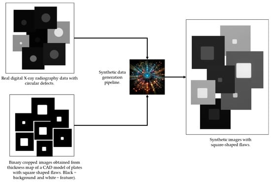
In our approach, we chose to use binary representation, as can be seen in the process chart in Figure 7, to define the target regions of interest to be used by the simulation pipeline for the determination of the feature and background. This is practicable because only two thicknesses are considered in each image. This binary representation was realized by thresholding a thickness map acquired from a CAD model with cuboidal features representing flat-bottom holes.
Figure 7.
High-level schematic representation of the processes involved in synthetic data generation.
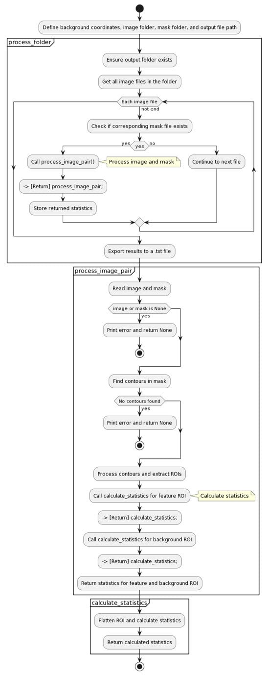
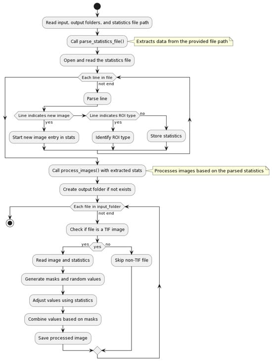
A detailed description of the synthetic data generation pipeline can be found in Figure A1 and Figure A2. Our statistical modeling approach ensures that the synthetic images reflect a realistic presentation of flaws, potentially enhancing the model’s applicability in digital X-ray radiography images. Additionally, this method allows for the creation of a large and diverse dataset, essential for the robust training of a deep learning model. Boundary characteristics between features and background are crucial for deep learning training. In real X-ray radiography acquisition, factors that worsen edge delineation include scatter radiation effects [40], the geometric configuration of the acquisition setup, penumbra formation resulting from the finite size of the focal spot [41], etc. To address this concern, in our synthetic images, we implemented a methodology that successfully mimics the edge characteristics observed in real X-ray images in our simulated images to potentially improve model performance. This was achieved by feathering the boundaries between features and background using the operations described as follows:
The Gaussian function utilized in our approach is two-dimensional to cover an area of pixel dimension. It is mathematically expressed by Equation (5), where is the standard deviation of the distribution, which controls the spread of the blur.
The convolution process for a point in the image is mathematically expressed in Equation (6).
Here, represents the original image, represents the intensity of the blurred image at the pixel location , and corresponds to the kernel size. indicates the value from the Gaussian kernel at position , while represents the intensity of the original image at a location offset by from . The sums over and iterate over the kernel size, which is defined by . For the kernel, would be (as the kernel extends pixels in each direction from the center).
Furthermore, it was essential to scale the blurred image to a range between and , inversely for the background and directly for the feature. This was achieved as expressed by Equations (7) and (8).
Finally, to achieve a blending of the background and feature regions of the synthetic data using these masks, the approach is mathematically expressed in Equation (9).
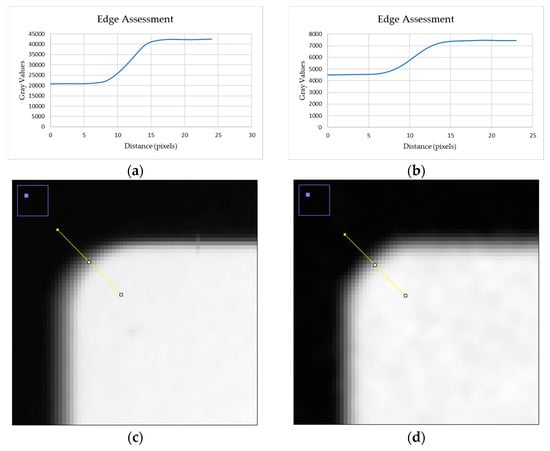
These operations ensure boundary transition between the background and feature to mimic what is obtainable in real X-ray radiography images. A comparison of real and synthetic data is described in Figure 8.
Figure 8.
(a) Shows line profile pixel intensity readings represented by the yellow line across the edge of the zoomed-in X-ray radiography image presented in (c); while image (b) shows line profile pixel intensity readings represented by the yellow line in across the edge of the zoomed-in synthetic image in (d).
3.2. Deep Learning Model Training
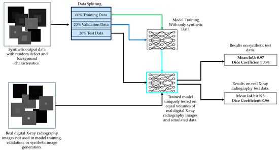
YOLOv8, an acronym for You Only Look Once version 8, is a state-of-the-art deep learning model designed for real-time object detection, image segmentation, and classification tasks [42]. It is known for its efficiency and speed in processing images. YOLOv8 incorporates a deep neural network architecture, combining the advantages of the YOLO framework with advancements in model design and training strategies. The model utilizes a single neural network to simultaneously predict bounding boxes, object classes, and segmentation masks for each detected object within an input image. The architecture is built upon a backbone of convolutional layers, enabling it to effectively capture hierarchical features in images. To train the model, we utilized pre-trained weights from yolov8n with about 3.4 million parameters, which was trained on the COCO dataset [43]. This implies that the initial weights used for training were not random. This transfer-learning approach was chosen in a bid to facilitate the training of the model with our purely synthetic data. A single class, called FB_Hole, was used, which represented the square-shaped features in both the synthetically generated dataset used for the training and the real X-ray radiography test data. A schematic description of the model training approach adopted in this study is presented in Figure 9.
Figure 9.
Model training description, showing the neural network trained on only synthetic data and tested two distinct times on both synthetic and real test data.
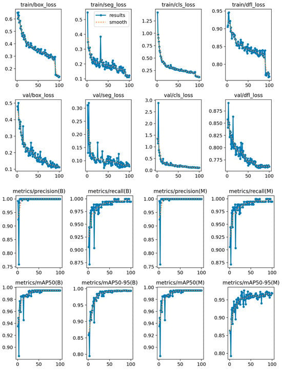
The model was trained for a total of 100 epochs, where the performance of the best-trained model was tested on real X-ray radiography images that were not included in either the training or validation datasets and compared the result with the model’s performance on synthetic data not included in either the training or validation data. Relevant training metrics are presented in Figure 10 and Figure 11.
Figure 11.
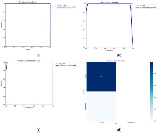
(a) Precision–Recall curve (b) F1-Confidence score (c) Precision-Confidence curve (d) Confusion Matrix.
From the charts provided in Figure 11, the model achieved near-perfect precision and recall across the dataset, which indicates that it can correctly identify and segment the target flaws (FB_Hole) with high reliability. It could also be observed that the F1 score remains high across all confidence levels, indicating a strong balance between precision and recall. Furthermore, the mean Average Precision scores are extremely high (around 0.995), demonstrating the model’s ability to accurately predict bounding boxes and segmentation. Additionally, our model trained relatively quickly, completing 100 epochs in 0.825 h, which is a considerably rapid training time that is indicative of an efficient training process, likely aided by the powerful Tesla T4 GPU used for training. A look at the loss metrics reveals a steady decrease over training epochs, reflecting the model’s learning efficacy and stability, and suggesting robustness against overfitting. Another striking observation is the model’s inference time, averaging at about 8.0 ms per image, hence making it remarkably fast and suitable for real-time applications. Moreover, the striped-down trained weight file is only 6.8 MB, which is small and further adds to the practicability of integrating the trained model into systems that require fast, accurate object detection and segmentation. A potential example is real-time automated defect recognition (ADR) solutions for digital X-ray radiography applications.
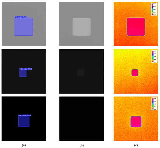
Figure 12 shows a cross-section of the results of the model performance on real X-ray radiography images. Apart from the prediction results and associated original images, corresponding color spectrum images are also presented to appreciate visually the inhomogeneous gray value distribution in the images.
Figure 12.
A cross-section of results of the model performance on real X-ray radiography images. Images on the same row represent a single entry, with columns (a), representing prediction, (b) the original input image, and (c) a conversion of the input images to color spectrum for easier visualization of the pixel intensity distribution.
4. Discussion
One of the noteworthy offerings of this research work is the ability of our model, trained exclusively on synthetic data, to demonstrate remarkable generalization capabilities when applied to real-world digital X-ray radiography image data. Our approach of building a synthetic image generation pipeline that incorporates the statistical characteristics of real X-ray images ensures that the synthetic data not only mimics these statistical properties of the real-world X-ray radiography images but also the nuances and complexities present in such real X-ray radiography images. Since the generalization of our trained model is at the core of our interest, for the synthetic data, we used a different morphological representation (square-shaped features) compared to the circular features of the dataset analyzed for the extraction of statistical parameters. Additionally, for the real X-ray radiography test images that were used to evaluate the model’s performance, a random selection of images was made from a dataset of 900 cropped images that were acquired with 20 different exposure conditions. These images had square feature representations that varied in gray values due to the differing thicknesses of the flat-bottom holes in the imaged aluminum plates. Notwithstanding the measures employed, the trained model attained a mean IoU of 0.93 and a mean dice coefficient of 0.96, showcasing the effectiveness of our synthetic data generation approach and underscoring the adaptability of the same in industrial contexts, particularly those involving manufactured components of similar dimensions.
5. Conclusions and Future Work
In conclusion, our research contributes to the growing body of evidence supporting the efficacy of synthetic data in training deep-learning models. The unique integration of the statistical distribution of intensity values, as seen in real X-ray radiography images, into the simulation pipeline in the manner expressed in this work represents a unique approach that enhances the deep learning model’s ability to generalize to real-world scenarios. By adopting our approach to industries that fabricate components with similar dimensions (such as the aluminum die-casting industry), we envision a revolution in quality assurance processes involving digital X-ray radiography inspections. As industries continue to embrace automated defect recognition (ADR), our methodology has the potential to become pivotal in ensuring consistent and high-quality assessment of digital X-ray radiography images of manufactured components.
While our approach has demonstrated promising advancements, it is essential to acknowledge its current limitations, particularly in terms of the generalizability of our synthetic X-ray radiography image generation pipeline to very complex geometries. This recognition of constraints lays the foundation for future research and improvement. As part of our future work, we intend to focus on addressing these limitations by incorporating methodologies specifically designed to accommodate complex geometries. This includes the further exploration of modeling techniques to address edge variations and geometry-induced scattering effects in curved structures.
Author Contributions
Conceptualization, B.H.; methodology, B.H.; software, B.H.; validation, B.H. and Z.W.; formal analysis, B.H., Z.W. and L.P.; investigation, B.H.; data curation, B.H.; writing—original draft preparation, B.H.; writing—review and editing, C.I.C.; supervision, C.I.C. and X.M.; funding acquisition, X.M. All authors have read and agreed to the published version of the manuscript.
Funding
The authors wish to acknowledge the support of the Natural Sciences and Engineering Council of Canada (NSERC), CREATE-oN DuTy! Program (funding reference number 496439-2017), the Mitacs Acceleration program (funding reference FR49395), the Canada Research Chair in Multi-polar Infrared Vision (MIVIM), and the Canada Foundation for Innovation.
Data Availability Statement
Data could be provided upon request through the corresponding author.
Acknowledgments
We thankfully acknowledge the support and collaboration provided by Gilab Solutions, Quebec City, Canada.
Conflicts of Interest
Author Luc Perron was employed by GI Lab Solutions, Quebec City, Canada. The remaining authors declare that the research was conducted in the absence of any commercial or financial relationships that could be construed as a potential conflict of interest.
References
- Chen, Z.-H.; Juang, J.-C. YOLOv4 Object Detection Model for Nondestructive Radiographic Testing in Aviation Maintenance Tasks. AIAA J. 2021, 60, 526–531. [Google Scholar] [CrossRef]
- Misokefalou, D.; Papoutsidakis, P.; Priniotakis, P. Non-Destructive Testing for Quality Control in Automotive Industry. IJEAST 2022, 7, 349–355. [Google Scholar] [CrossRef]
- Parlak, İ.E.; Emel, E. Deep Learning-Based Detection of Aluminum Casting Defects and Their Types. Eng. Appl. Artif. Intell. 2023, 118, 105636. [Google Scholar] [CrossRef]
- Beránek, L.; Kroisová, D.; Dvořáčková, Š.; Urban, J.; Šimota, J.; Andronov, V.; Bureš, L.; Pelikán, L. Use of Computed Tomography in Dimensional Quality Control and NDT. Manuf. Technol. 2020, 20, 566–575. [Google Scholar] [CrossRef]
- Baur, M.; Uhlmann, N.; Pöschel, T.; Schröter, M. Correction of Beam Hardening in X-ray Radiograms. Rev. Sci. Instrum. 2019, 90, 025108. [Google Scholar] [CrossRef] [PubMed]
- Aral, N.; Amor Duch, M.; Banu Nergis, F.; Candan, C. The Effect of Tungsten Particle Sizes on X-ray Attenuation Properties. Radiat. Phys. Chem. 2021, 187, 109586. [Google Scholar] [CrossRef]
- Ou, X.; Chen, X.; Xu, X.; Xie, L.; Chen, X.; Hong, Z.; Bai, H.; Liu, X.; Chen, Q.; Li, L.; et al. Recent Development in X-ray Imaging Technology: Future and Challenges. Research 2021, 2021, 9892152. [Google Scholar] [CrossRef]
- Say, D.; Zidi, S.; Qaisar, S.M.; Krichen, M. Automated Categorization of Multiclass Welding Defects Using the X-ray Image Augmentation and Convolutional Neural Network. Sensors 2023, 23, 6422. [Google Scholar] [CrossRef]
- Standard Terminology for Nondestructive Examinations. Available online: https://www.astm.org/e1316-17a.html (accessed on 5 December 2023).
- Luo, A.A.; Sachdev, A.K.; Apelian, D. Alloy Development and Process Innovations for Light Metals Casting. J. Mater. Process. Technol. 2022, 306, 117606. [Google Scholar] [CrossRef]
- Mazzei, D.; Ramjattan, R. Machine Learning for Industry 4.0: A Systematic Review Using Deep Learning-Based Topic Modelling. Sensors 2022, 22, 8641. [Google Scholar] [CrossRef]
- Fascista, A.; Coluccia, A.; Ravazzi, C. A Unified Bayesian Framework for Joint Estimation and Anomaly Detection in Environmental Sensor Networks. IEEE Access 2023, 11, 227–248. [Google Scholar] [CrossRef]
- Lazzaretti, A.E.; Costa, C.H.D.; Rodrigues, M.P.; Yamada, G.D.; Lexinoski, G.; Moritz, G.L.; Oroski, E.; Goes, R.E.D.; Linhares, R.R.; Stadzisz, P.C.; et al. A Monitoring System for Online Fault Detection and Classification in Photovoltaic Plants. Sensors 2020, 20, 4688. [Google Scholar] [CrossRef] [PubMed]
- Lindgren, E.; Zach, C. Industrial X-ray Image Analysis with Deep Neural Networks Robust to Unexpected Input Data. Metals 2022, 12, 1963. [Google Scholar] [CrossRef]
- García Pérez, A.; Gómez Silva, M.J.; De La Escalera Hueso, A. Automated Defect Recognition of Castings Defects Using Neural Networks. J. Nondestruct. Eval. 2022, 41, 11. [Google Scholar] [CrossRef]
- Tyystjärvi, T.; Virkkunen, I.; Fridolf, P.; Rosell, A.; Barsoum, Z. Automated Defect Detection in Digital Radiography of Aerospace Welds Using Deep Learning. Weld World 2022, 66, 643–671. [Google Scholar] [CrossRef]
- Gabelica, M.; Bojčić, R.; Puljak, L. Many Researchers Were Not Compliant with Their Published Data Sharing Statement: A Mixed-Methods Study. J. Clin. Epidemiol. 2022, 150, 33–41. [Google Scholar] [CrossRef] [PubMed]
- Meyendorf, N.; Ida, N.; Singh, R.; Vrana, J. NDE 4.0: Progress, Promise, and Its Role to Industry 4.0. NDT E Int. 2023, 140, 102957. [Google Scholar] [CrossRef]
- Jiangsha, A.; Tian, L.; Bai, L.; Zhang, J. Data Augmentation by a CycleGAN-Based Extra-Supervised Model for Nondestructive Testing. Meas. Sci. Technol. 2022, 33, 045017. [Google Scholar] [CrossRef]
- Yosifov, M.; Reiter, M.; Heupl, S.; Gusenbauer, C.; Fröhler, B.; Fernández- Gutiérrez, R.; De Beenhouwer, J.; Sijbers, J.; Kastner, J.; Heinzl, C. Probability of Detection Applied to X-ray Inspection Using Numerical Simulations. Nondestruct. Test. Eval. 2022, 37, 536–551. [Google Scholar] [CrossRef]
- Bellon, C.; Deresch, A.; Gollwitzer, C.; Jaenisch, G.-R. Radiographic Simulator aRTist: Version 2. In Proceedings of the 18th WCNDT—World Conference on Nondestructive Testing, Durban, South Africa, 16–20 April 2012. [Google Scholar]
- Giersch, J.; Durst, J. Monte Carlo Simulations in X-ray Imaging. Nucl. Instrum. Methods Phys. Res. Sect. A Accel. Spectrometers Detect. Assoc. Equip. 2008, 591, 300–305. [Google Scholar] [CrossRef]
- Ivanovs, M.; Ozols, K.; Dobrajs, A.; Kadikis, R. Improving Semantic Segmentation of Urban Scenes for Self-Driving Cars with Synthetic Images. Sensors 2022, 22, 2252. [Google Scholar] [CrossRef] [PubMed]
- Kortylewski, A.; Schneider, A.; Gerig, T.; Egger, B.; Morel-Forster, A.; Vetter, T. Training Deep Face Recognition Systems with Synthetic Data. arXiv 2018, arXiv:1802.05891. [Google Scholar]
- Penekalapati, S.V.; Ramana, E.V.; Kumar, N.K. Automatic Detection of Sub-Surface Weld Defects Using Machine Learning Approach. In Proceedings of the 2022 International Conference on Recent Trends in Microelectronics, Automation, Computing and Communications Systems (ICMACC), Hyderabad, India, 28–30 December 2022; IEEE: Hyderabad, India, 2022; pp. 412–415. [Google Scholar]
- Bosse, S.; Lehmhus, D. Automated Detection of Hidden Damages and Impurities in Aluminum Die Casting Materials and Fibre-Metal Laminates Using Low-Quality X-ray Radiography, Synthetic X-ray Data Augmentation by Simulation, and Machine Learning. arXiv 2023, arXiv:2311.12041. [Google Scholar]
- Bosse, S. Automated Damage and Defect Detection with Low-Cost X-ray Radiography Using Data-Driven Predictor Models and Data Augmentation by X-ray Simulation. Eng. Proc. 2023, 56. [Google Scholar]
- Dong, X.; Taylor, C.J.; Cootes, T.F. Automatic Aerospace Weld Inspection Using Unsupervised Local Deep Feature Learning. Knowl.-Based Syst. 2021, 221, 106892. [Google Scholar] [CrossRef]
- Kumar, A.; Arnold, W. High Resolution in Non-Destructive Testing: A Review. J. Appl. Phys. 2022, 132, 100901. [Google Scholar] [CrossRef]
- Olivo, A. Edge-Illumination X-ray Phase-Contrast Imaging. J. Phys. Condens. Matter 2021, 33, 363002. [Google Scholar] [CrossRef]
- Kusk, M.W.; Jensen, J.M.; Gram, E.H.; Nielsen, J.; Precht, H. Anode Heel Effect: Does It Impact Image Quality in Digital Radiography? A Systematic Literature Review. Radiography 2021, 27, 976–981. [Google Scholar] [CrossRef]
- Qiao, C.-K.; Wei, J.-W.; Chen, L. An Overview of the Compton Scattering Calculation. Crystals 2021, 11, 525. [Google Scholar] [CrossRef]
- Sayed, M.; Knapp, K.M.; Fulford, J.; Heales, C.; Alqahtani, S.J. The Principles and Effectiveness of X-ray Scatter Correction Software for Diagnostic X-ray Imaging: A Scoping Review. Eur. J. Radiol. 2023, 158, 110600. [Google Scholar] [CrossRef]
- Hong, J.; Binzel, R.P.; Allen, B.; Guevel, D.; Grindlay, J.; Hoak, D.; Masterson, R.; Chodas, M.; Lambert, M.; Thayer, C.; et al. Calibration and Performance of the REgolith X-ray Imaging Spectrometer (REXIS) Aboard NASA’s OSIRIS-REx Mission to Bennu. Space Sci. Rev. 2021, 217, 83. [Google Scholar] [CrossRef]
- Standard Practice for Manufacturing Characterization of Digital Detector Arrays. Available online: https://www.astm.org/e2597_e2597m-22.html (accessed on 5 December 2023).
- Gutiérrez, C.E.; Sabra, A. The Reflector Problem and the Inverse Square Law. Nonlinear Anal. Theory Methods Appl. 2014, 96, 109–133. [Google Scholar] [CrossRef][Green Version]
- Hena, B.; Wei, Z.; Castanedo, C.I.; Maldague, X. Deep Learning Neural Network Performance on NDT Digital X-ray Radiography Images: Analyzing the Impact of Image Quality Parameters—An Experimental Study. Sensors 2023, 23, 4324. [Google Scholar] [CrossRef] [PubMed]
- Xiao, Z.; Song, K.-Y.; Gupta, M.M. Development of a CNN Edge Detection Model of Noised X-ray Images for Enhanced Performance of Non-Destructive Testing. Measurement 2021, 174, 109012. [Google Scholar] [CrossRef]
- Kuang, Y. (Ed.) Principles and Practice of Image-Guided Abdominal Radiation Therapy; IOP Publishing: Bristol, UK, 2023; ISBN 978-0-7503-2468-7. [Google Scholar]
- Graetz, J.; Balles, A.; Hanke, R.; Zabler, S. Review and Experimental Verification of X-ray Dark-Field Signal Interpretations with Respect to Quantitative Isotropic and Anisotropic Dark-Field Computed Tomography. Phys. Med. Biol. 2020, 65, 235017. [Google Scholar] [CrossRef]
- Momose, A. X-ray Phase Imaging Reaching Clinical Uses. Physica Medica 2020, 79, 93–102. [Google Scholar] [CrossRef]
- Terven, J.; Córdova-Esparza, D.-M.; Romero-González, J.-A. A Comprehensive Review of YOLO Architectures in Computer Vision: From YOLOv1 to YOLOv8 and YOLO-NAS. Mach. Learn. Knowl. Extr. 2023, 5, 1680–1716. [Google Scholar] [CrossRef]
- Lin, T.-Y.; Maire, M.; Belongie, S.; Hays, J.; Perona, P.; Ramanan, D.; Dollár, P.; Zitnick, C.L. Microsoft COCO: Common Objects in Context. In Proceedings of the Computer Vision–ECCV 2014: 13th European Conference, Zurich, Switzerland, 6–12 September 2014; pp. 740–755. [Google Scholar]
Disclaimer/Publisher’s Note: The statements, opinions and data contained in all publications are solely those of the individual author(s) and contributor(s) and not of MDPI and/or the editor(s). MDPI and/or the editor(s) disclaim responsibility for any injury to people or property resulting from any ideas, methods, instructions or products referred to in the content. |
© 2023 by the authors. Licensee MDPI, Basel, Switzerland. This article is an open access article distributed under the terms and conditions of the Creative Commons Attribution (CC BY) license (https://creativecommons.org/licenses/by/4.0/).
