Abstract
Within the domain of architectural urban informatization, the automated precision recognition of two-dimensional paper schematics emerges as a pivotal technical challenge. Recognition methods traditionally employed frequently encounter limitations due to the fluctuating quality of architectural drawings and the bounds of current image processing methodologies, inhibiting the realization of high accuracy. The research delineates an innovative framework that synthesizes refined semantic segmentation algorithms with image processing techniques and precise coordinate identification methods, with the objective of enhancing the accuracy and operational efficiency in the identification of architectural elements. A meticulously curated data set, featuring 13 principal categories of building and structural components, facilitated the comprehensive training and assessment of two disparate deep learning models. The empirical findings reveal that these algorithms attained mean intersection over union (MIoU) values of 96.44% and 98.01% on the evaluation data set, marking a substantial enhancement in performance relative to traditional approaches. In conjunction, the framework’s integration of the Hough Transform with SQL Server technology has significantly reduced the coordinate detection error rates for linear and circular elements to below 0.1% and 0.15%, respectively. This investigation not only accomplishes the efficacious transition from analog two-dimensional paper drawings to their digital counterparts, but also assures the precise identification and localization of essential architectural components within the digital image coordinate framework. These developments are of considerable importance in furthering the digital transition within the construction industry and establish a robust foundation for the forthcoming extension of data collections and the refinement of algorithmic efficacy.
1. Introduction
Prior to the establishment of Computer-Aided Design (CAD) technologies, architectural design relied heavily upon the manual creation of blueprints—a practice that has become increasingly obsolete in the era of progressive urban informatization. The integration of CAD systems has markedly advanced the discipline of architectural design; however, the assimilation of pre-existing structures into contemporary urban information management systems poses significant challenges [1,2]. The static locations and intricate configurations of these structures require modifications to meet the dynamic technical and social demands, thereby imposing advanced requisites on extant technological solutions. The precision of CAD blueprints is imperative for the development of accurate Building Information Models (BIM) [3], which not only enhance the informatization retrofitting of pre-existing structures, but also serve as a cornerstone for intelligent building management systems. The transformation of analog blueprints into digital BIM frameworks, however, is fraught with complexity and inefficiency, primarily due to the difficulty in accurately extracting component classifications and pivotal coordinates from these documents. The predominant method involves the digitization of physical blueprints via scanning, followed by labor-intensive manual adjustments within CAD software, a process that is both time-consuming and susceptible to human error. In light of this, the urgent development of an algorithm capable of swiftly and precisely discerning component categories and essential coordinates from paper blueprints has emerged as a critical imperative.
In the realm of computer vision, the implementation of deep learning methodologies has engendered profound breakthroughs, with wide-reaching implications across multiple scientific domains, including architecture, medicine, and materials science [4,5,6,7,8,9]. Semantic segmentation, deemed a pivotal endeavor within computer vision, endeavors to delineate images and assign semantic labels to each constituent pixel, drawing upon an established taxonomy of tags [10]. This task transcends the capabilities of mere image classification or object recognition by furnishing a granular perspective on the image content, thus facilitating an advanced level of interpretative analysis. A plethora of algorithms, such as FCN, PSPNet, U-Net, SegNet, the Deeplab series, Transformer, and notably SegFormer, have been developed to address this intricate task [11,12,13,14,15,16,17,18]. Within the sphere of civil engineering, and more specifically in the identification of structural defects, the application of semantic segmentation algorithms has demonstrated superior performance [19,20,21,22,23,24,25]. The research presented herein utilizes the SegFormer network, which is predicated on the Transformer design paradigm, expressly conceived for the exigent task of pixel-level image segmentation. Empirical studies corroborate that the SegFormer model, in conjunction with other transformative enhancements upon the Transformer framework, plays a critical role in propelling the evolution of semantic segmentation models towards heightened efficiency [9,26].
The fidelity of blueprint identification is imperative for influencing the extraction of architectural parameters and the caliber of downstream applications. The scholarly discourse to date has predominantly addressed the delineation of component outlines within blueprints, resulting in the advent of assorted recognition methodologies. Methods predicated on the discernment of contours and edges have been shown to proficiently capitalize on the inherent regularity of line segments and the salient edge details present in bidimensional blueprints [27,28,29]. The application of graph theory, moreover, has facilitated the transposition of architectural drawing components into actionable spatial and topological data [30]. In the realm of facade blueprints, investigative efforts have been directed toward the analysis and taxonomy of stratified content, including the accurate discernment of elevations, thereby yielding a suite of innovative categorization techniques for architectural stratification [31]. The pervasive deployment of deep learning modalities, especially within the recognition of three-dimensional CAD models, has demonstrated considerable promise for augmenting the precision of twofold blueprint detection [32,33]. Recent interdisciplinary investigations have seen a surge in the confluence of machine vision and architectural engineering schematics. A novel approach by Zhao et al. [34] amalgamates hybrid image processing, targeted detection, and Optical Character Recognition (OCR) to extract entity information from structural imagery. Concurrently, Pan et al. [35] have pioneered a technique that integrates instance segmentation with semantically augmented image processing, specifically tailored for the identification of pipeline blueprints and the restoration of BIM frameworks in the IFC standard.
While foundational research has established a platform for blueprint recognition, these incumbent methodologies are marred by inefficiencies. Presently, deep learning has exhibited notable utility in two-dimensional blueprint detection, yet its practical deployment is constricted, with particular deficits in the detection of component coordinates—a domain where the efficacious harnessing of deep learning remains inadequately addressed. Therefore, the present investigation introduces an innovative approach that synthesizes the SegFormer semantic segmentation network model with advanced image processing techniques, endeavoring to actualize the potential of sophisticated deep learning applications in the semantic segmentation of architectural blueprints. Empirical evaluations substantiate that the proposed methodology facilitates the precise and efficient extraction of CAD components and their coordinates from scanned blueprints, markedly refining the intricacy and temporal efficiency associated with the recognition and transformation of bidimensional blueprints.
The structure of this manuscript is organized in the following manner. Section 2 delineates the research methodology with comprehensive detail. Section 3 constructs the experimental framework and furnishes the pertinent data sets. In Section 4, the findings are elucidated, and an analysis of the conclusions is undertaken, coupled with an examination of potential variables influencing the outcomes. The concluding section synthesizes the investigation, articulating the merits and scholarly contributions of this endeavor, and suggests trajectories for prospective inquiry.
2. Methodology
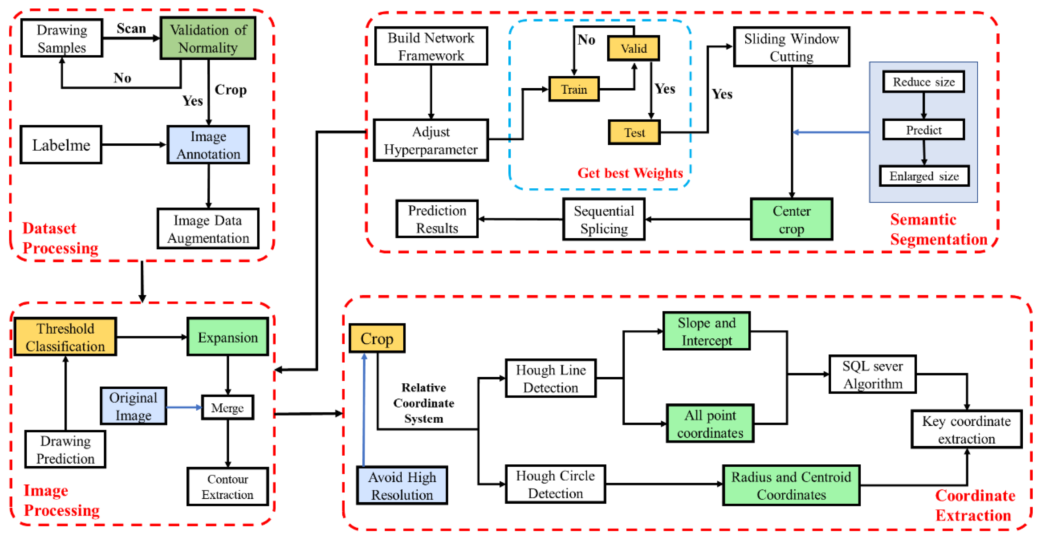
This section delineates the architecture of the SegFormer semantic segmentation network and the generation of a novel data set, examining the processing of semantic information in identified images and methods for coordinate extraction. The methodology is implemented in four distinct stages, as detailed in Figure 1.
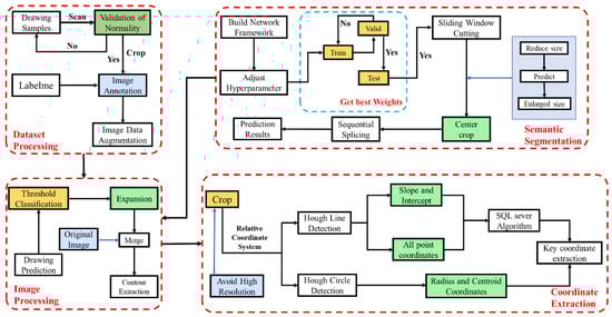
Figure 1.
Schematic diagram illustrating the comprehensive implementation of the proposed approach.
2.1. SegFormer Network
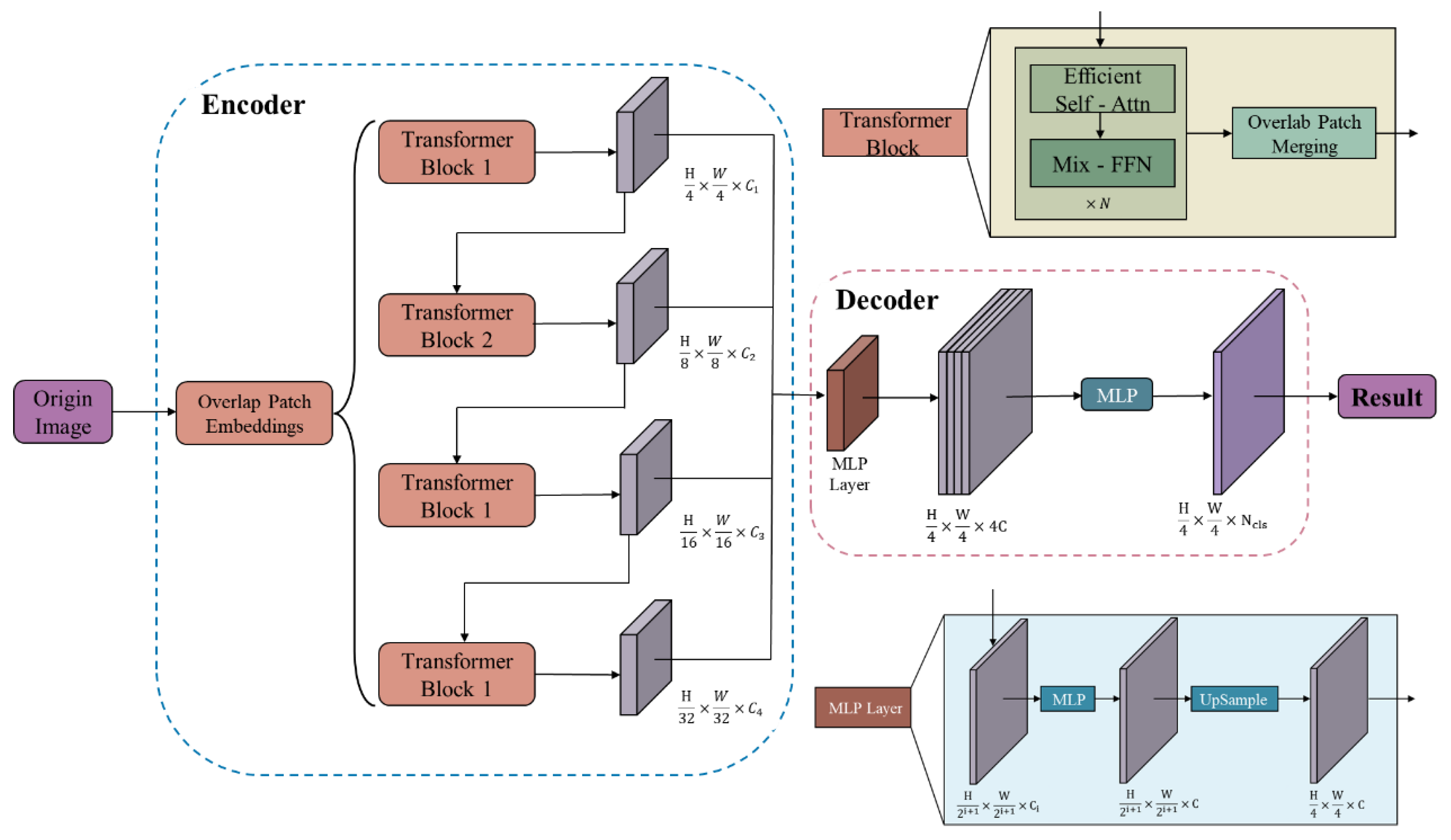
Figure 2 illustrates the SegFormer network’s utilization of a lightweight Transformer architecture for semantic segmentation. Key advantages involve the following: generating multi-resolution features through Overlap Patch Embedding; incorporating positional data using Mix-FFN, obviating position encoding and maintaining stable performance across resolution variations; and employing a simple MLP decoder for feature fusion and prediction. Empirical evidence confirms the network’s proficiency and resilience in semantic segmentation tasks.

Figure 2.
Illustrative diagram of the SegFormer network architecture for semantic segmentation.
2.2. Data Set
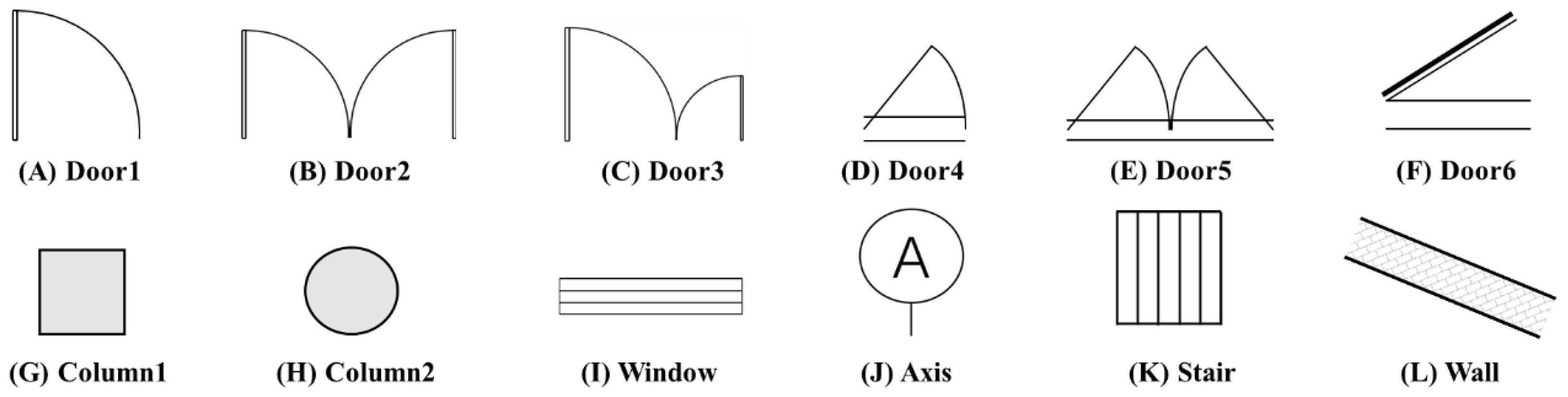
Semantic segmentation assigns distinct semantic meanings via diverse color labels, as illustrated in Figure 3 and Figure 4. The study categorizes 13 types of architectural and structural elements, comprising 12 architectural and 4 structural categories, with categories (G), (I), and (K) being common to both classifications.
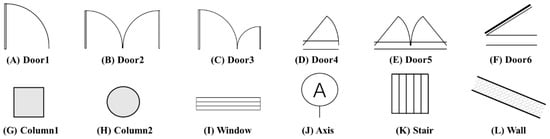
Figure 3.
Taxonomy of architectural components within the building sector.
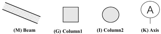
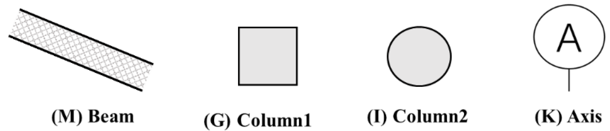
Figure 4.
Taxonomy of structural elements within the field of structural engineering.
The data set blueprints undergo conversion from two-dimensional formats into high-resolution pixel images, matching the deep learning network’s input size and computational limits to prevent overfitting due to resolution discrepancies. Images are resized as necessary using the Resize method with a gray bar to avoid distortion. The Labelme tool annotates these images, aligning labels precisely with component boundaries to produce images suitable for the semantic segmentation network.
2.2.1. Image Noise Reduction Processing
The data set’s original images undergo denoising to remove superfluous interference, termed ‘noise’, in the image data. Non-Local Means filtering, a denoising algorithm [36], is applied to prepare images for subsequent processing. The post-processed images comply with the established definition:
In Formula (1), represents the search area, and represents the weight, that is, the similarity between the , area blocks, usually represented by the Euclidean distance formula:
In Equation (2), is the normalization factor, defined as the sum of all weights, while acts as the filtering coefficient. This coefficient modulates the influence of Euclidean distance by controlling the rate of exponential decay. The term signifies the Gaussian-weighted Euclidean distance between adjacent regions and , where denotes the standard deviation of the Gaussian kernel. The algorithm’s efficacy lies in its capacity for full-image denoising, proficiently eliminating Gaussian noise across the image.
2.2.2. Adaptive Augmentation for Image Data Set Optimization
Adaptive image augmentation, which randomly transforms the original image to expand the training data set, enhances model robustness and mitigates overfitting. Changes in the original image’s size, flip, or rotation necessitate corresponding adjustments to the labels, whereas the label map remains invariant to image parameter alterations. The methods for this augmentation are detailed in Table 1.

Table 1.
Overview of image augmentation techniques applied to the data set.
2.3. Coordinate System Processing
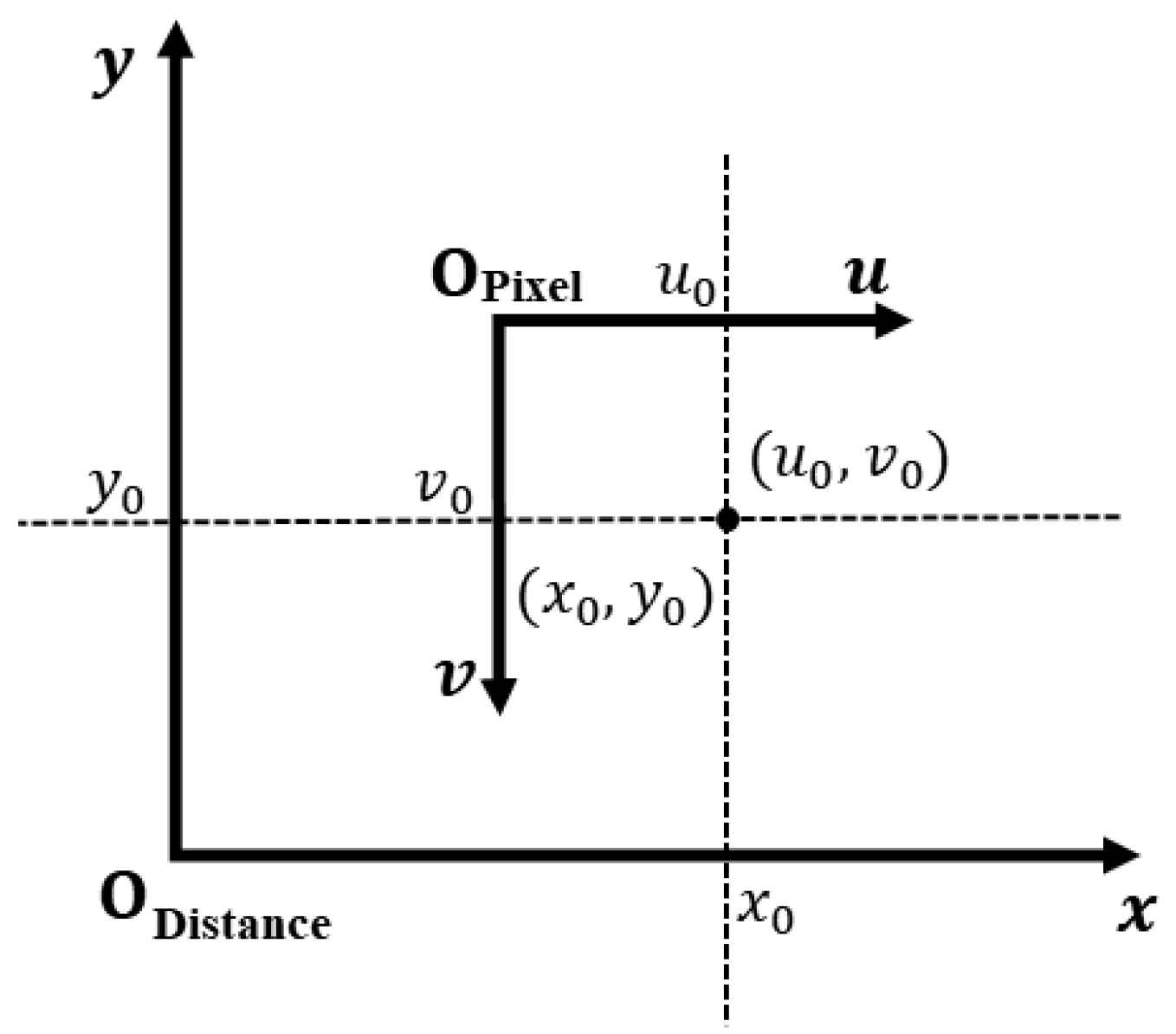
In the pixel map, pixel count represents length, whereas a separate coordinate system quantifies actual distance. A point on the pixel map is denoted by coordinates , while its equivalent on the actual blueprint is expressed as . The procedure to determine the conversion ratio between these systems is outlined as follows:
In Equation (3), and denote the X and Y coordinate conversion ratios, respectively. The coordinates (, , correspond to the initial points on the pixel map and the actual plane, while (, , represent the terminal points. To reduce errors, a minimum pixel-to-actual-length ratio (px:mm) of 1:1 is required, with higher ratios yielding more precise conversions.
A discrepancy exists between the image coordinate system, which primarily operates in the fourth quadrant, and the actual coordinate system, which is centered on the first quadrant. The coordinate conversion methodology is depicted in Figure 5 and detailed in Equation (4):

Figure 5.
Illustrative diagram depicting the correlation between the pixel and real-world coordinate systems.
The term is defined as the total width of the image measured in millimeters. Coordinates (, and refer to the positions on the pixel map and the corresponding actual planar distances, respectively.
2.4. Image Processing
2.4.1. Semantic Segmentation Using the “Edge Expansion Sliding Window Cropping Method”
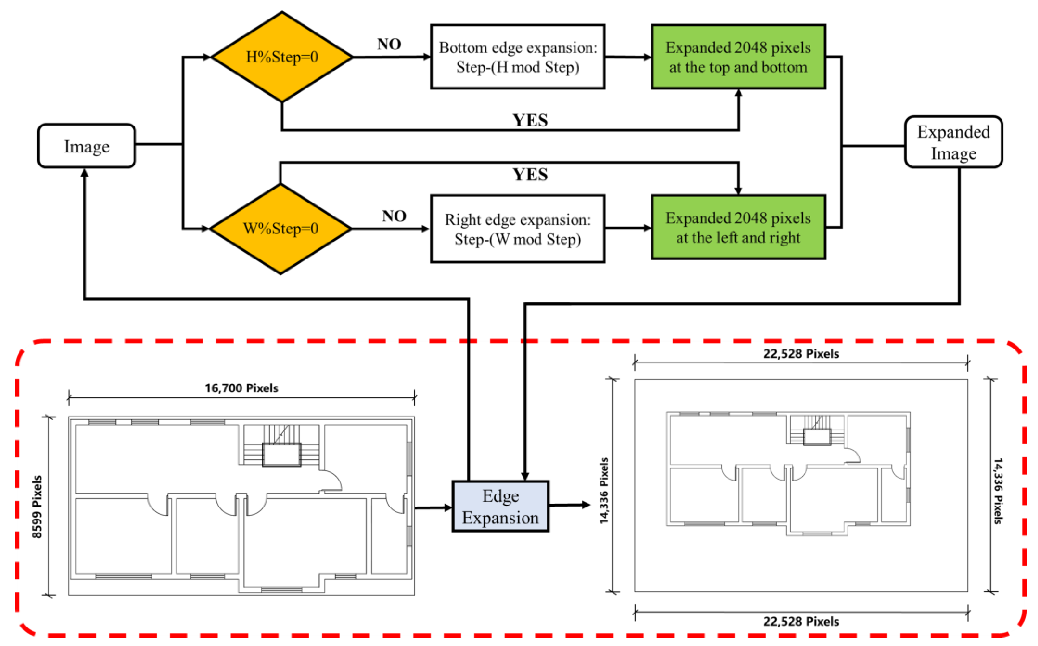
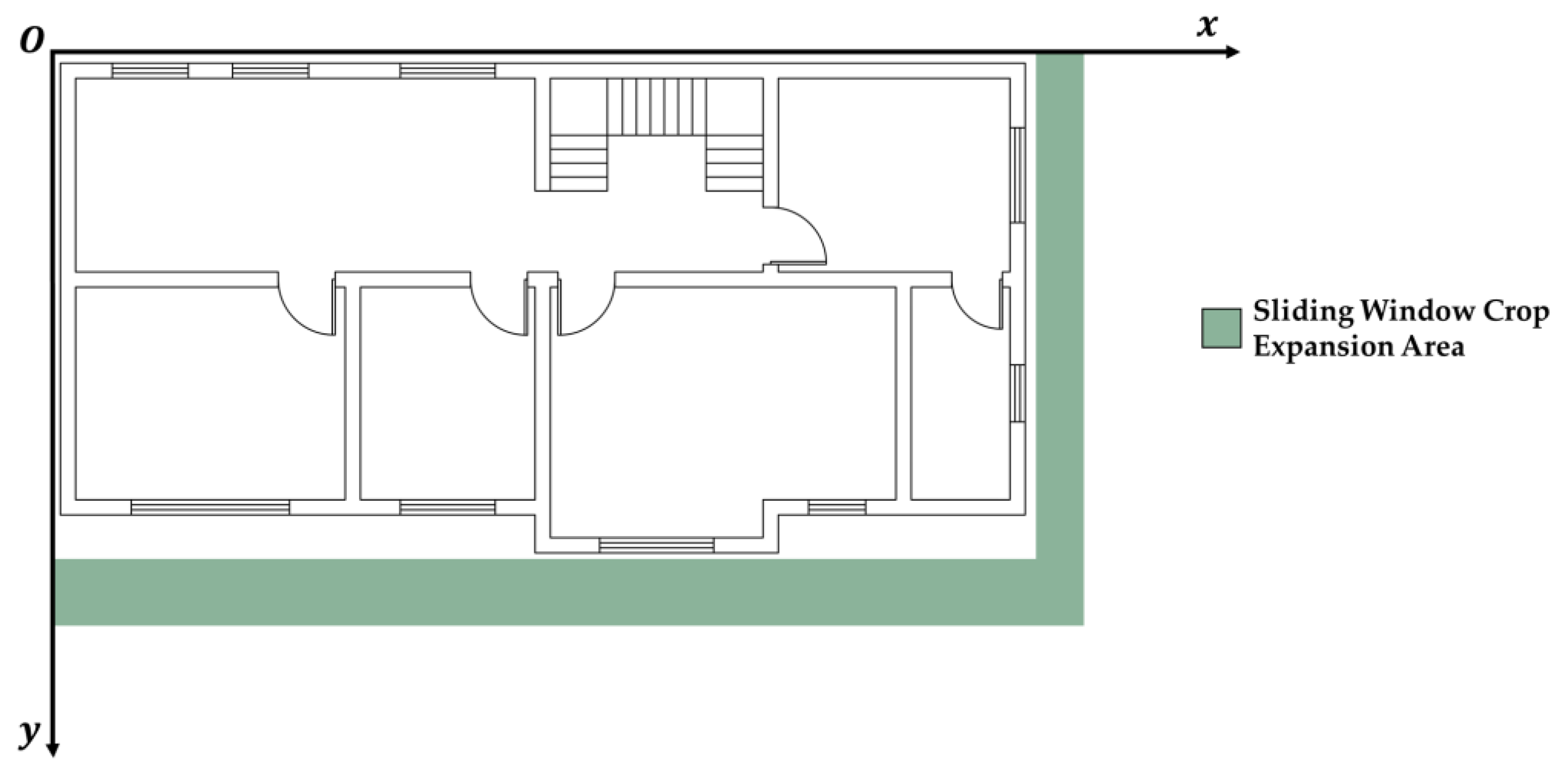
This study addresses semantic segmentation for high-resolution images. Standard cropping to facilitate prediction often neglects edge effects, risking errors when image borders cut through components. Disproportionate component sizes within the image also skew predictions. The introduced “Edge Expansion Sliding Window Cropping Method” combats these issues by extending image edges and padding with a white background, ensuring complete component capture. The method is detailed in Figure 6.
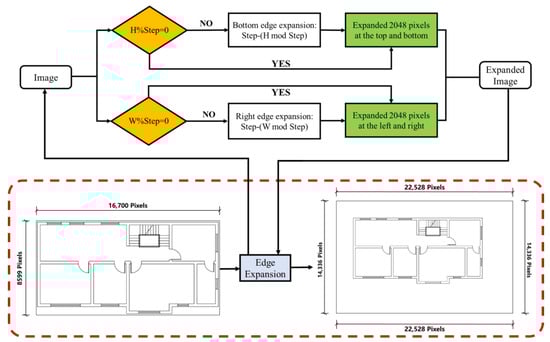
Figure 6.
Illustrative diagram of the process flow for edge expansion operations.
The image, once expanded, is processed using a sliding window crop of 2048-pixel steps, yielding windows of 6144 by 6144 pixels. This window size optimizes component area ratios, with expansions being step size multiples. Direct semantic segmentation is precluded by the sliding window technique, necessitating a resizing step. Resizing is achieved through nearest neighbor interpolation [37], assigning output pixel grayscale values based on their nearest input pixel counterparts. The transformation employs the following formula:
In Formula (5), and correspond to the pixel’s x and y coordinates, respectively, while and denote its width and height, respectively. Similarly, and pertain to the original image’s dimensions, and and indicate the original image’s coordinates that map to the point (, ) in the target image.
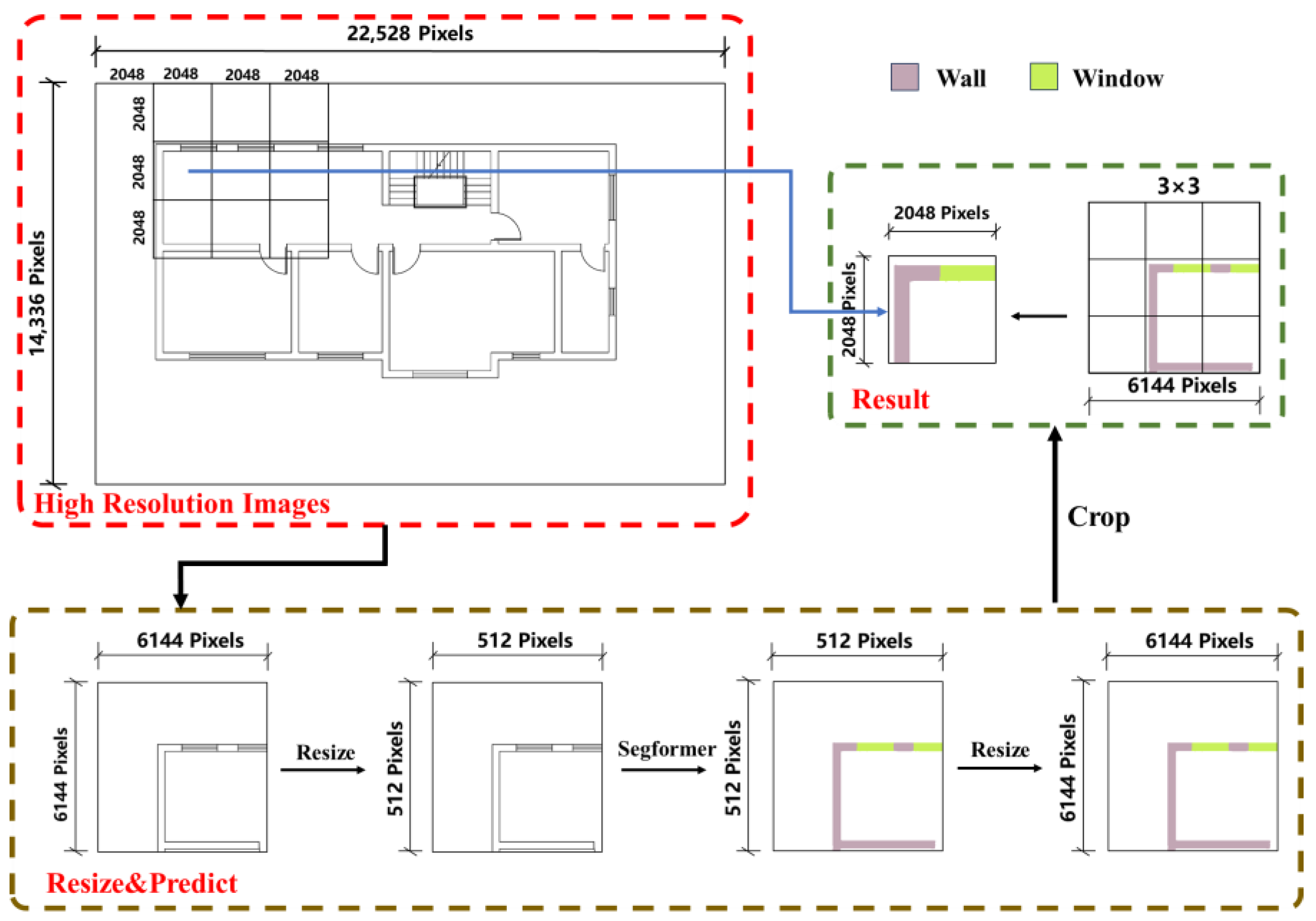
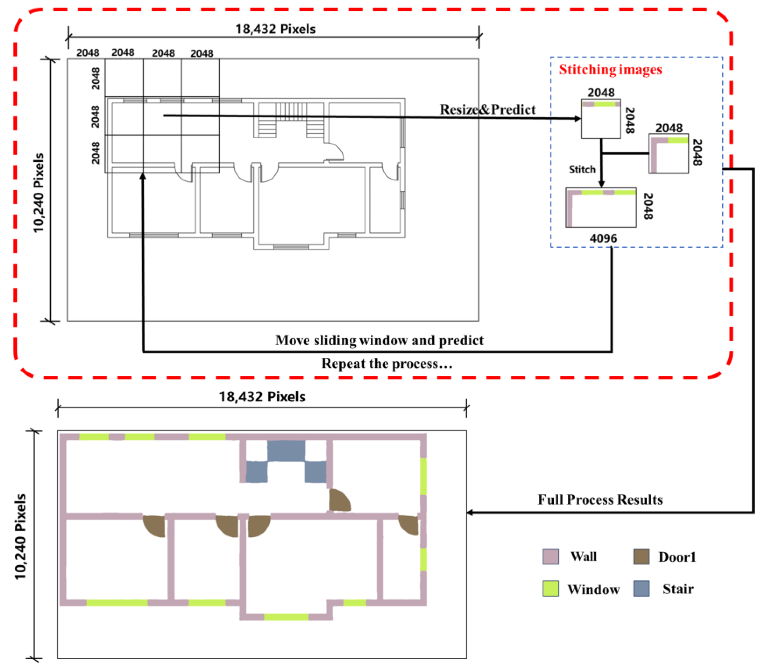
Images are downscaled to 512 × 512 pixels for the network model input as shown in Figure 7. Predicted outputs are then upscaled to 6144 × 6144 pixels using nearest neighbor interpolation, from which a 2048 × 2048-pixel central segment is extracted. The sliding window advances one step horizontally, and the procedure is repeated to secure a new central segment, which is immediately adjoined to the previous one. Upon reaching the image’s right boundary, the window descends a step and resumes leftward; this cycle continues until coverage is complete. The central segments are concatenated to form the final high-resolution semantic segmentation image, depicted in Figure 8.
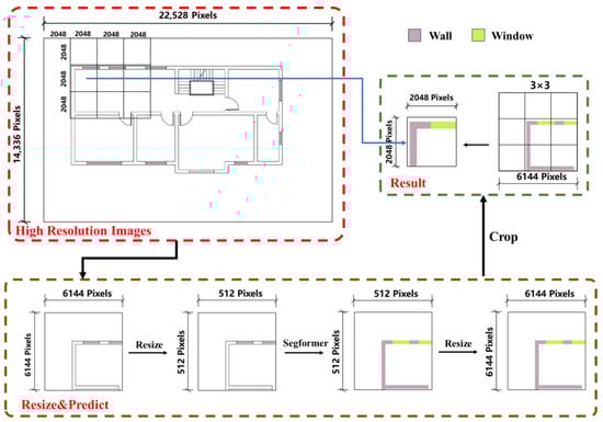
Figure 7.
Semantic segmentation using the ‘Sliding Window Cropping’ method.
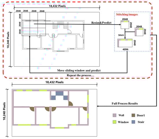
Figure 8.
Illustration of the execution flow for semantic segmentation applied to high-resolution image.
The method provides clear advantages. The expansion step in the image enlargement process ensures the original image’s initial frame is centered in the first sliding window, effectively preventing issues related to incomplete edge contours and maintaining the quality of the segmented image edges.
2.4.2. Classification and Contour Extraction Using Color Space
Semantic segmentation assigns unique colors to labels representing various semantics, with these values being predetermined. The present study applies these labels to extract particular features, ensuring that the resulting image maintains only these features at their original pixel locations.
The “Edge Expansion Sliding Window Cropping Method” ensures alignment between the coordinates of the original and the semantic segmentation images, allowing for their integrated processing. Through the Alpha Blending Method, the images are merged by modulating the blend ratios, yielding a composite image. In this process, the color semantics of the pixels within the original image’s contour are modified. Extraction of pixels is then performed in color space, with non-contour pixels removed, leaving only the desired component contours intact. Semantic segmentation thus acts as a means to delineate target contours from the original image without altering pixel coordinates.
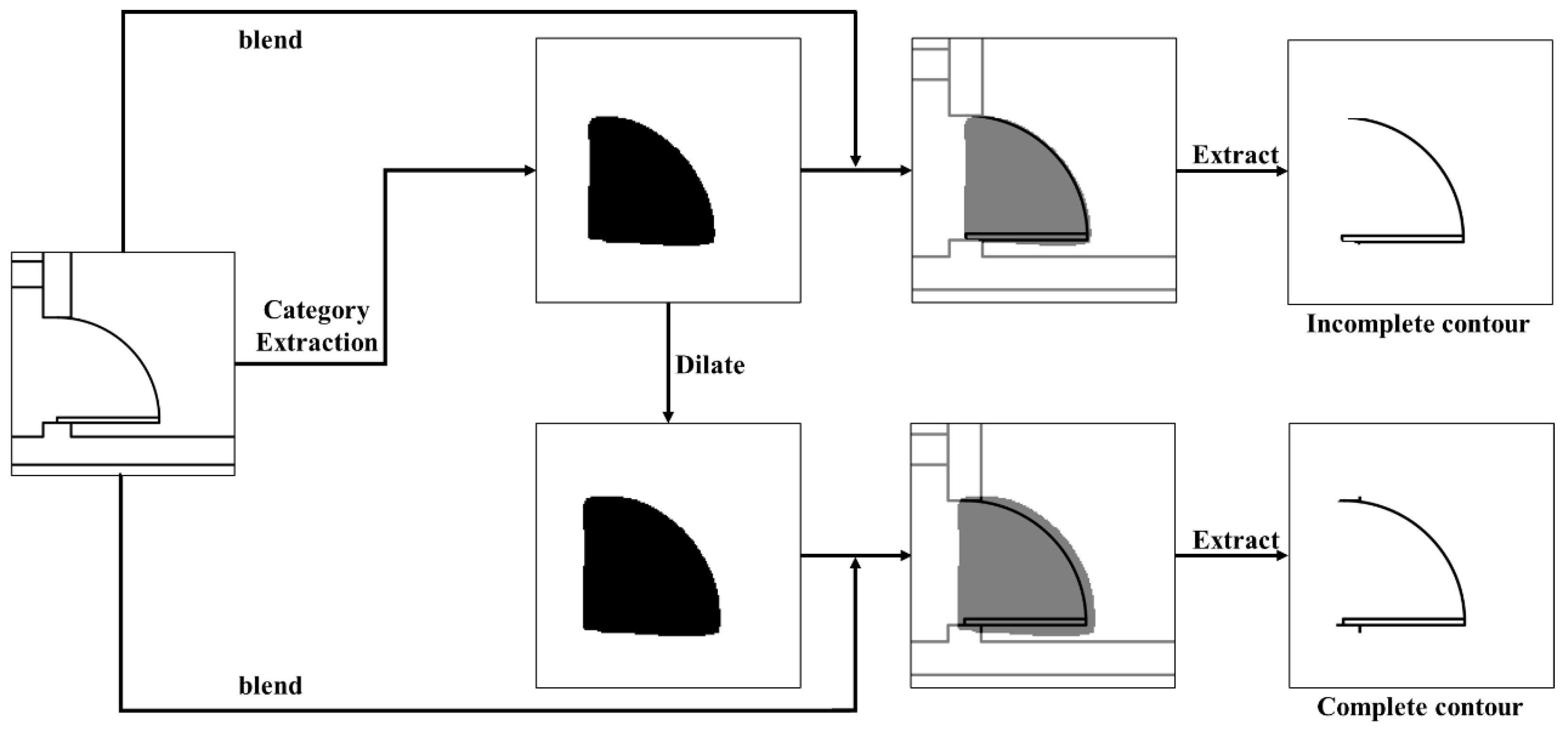
For component integrity, lines and arcs must be contiguous. Semantic segmentation may not fully capture contours, leading to inaccuracies like “dents” or “protrusions” (Figure 9). To address this, a dilation operation [38] fills gaps around the contour, ensuring complete coverage over the original contour. This operation replaces each pixel with the maximum value from its vicinity, with the dilation coefficient determined by component type.
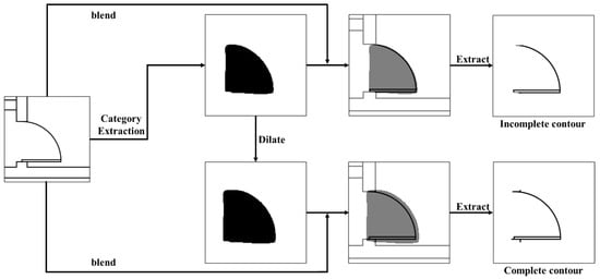
Figure 9.
Enhancement of semantic information areas via the dilation algorithm.
The process delineates the full contour of the target component. Contours are extracted globally and cropped locally to facilitate coordinate detection. Establishing the cropped image’s coordinate origin in relation to the full image is critical for precise detection. The process is depicted in Figure 10.
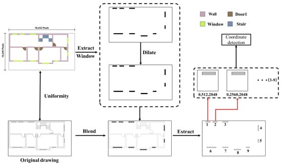
Figure 10.
Approach for deriving target component outlines employing threshold extraction and hybrid algorithms.
2.5. Hough Transform
2.5.1. Probabilistic Hough Line Detection
In two-dimensional blueprints, contours comprising line segments are critical for defining component positions. The Probabilistic Hough Line Detection method, an adaptation of the Hough Transform [39], efficiently detects these segments by sampling random edge points and filters out lines under a specified threshold, thereby optimizing detection precision for blueprint analysis.
Prior to Probabilistic Hough Line Detection, images are converted to grayscale to detect edges. For each edge, line parameters like slope and intercept are determined, and the most significant peak in the Hough space indicates the detected line, which is overlaid on the original image. The algorithm outputs coordinates, slopes, and intercepts of line segments; lines with zero or infinite slopes are handled by an SQL query algorithm. Key component coordinates are then extracted by importing data into the SQL Server for processing with the SQL algorithm.
2.5.2. Hough Circle Detection
The Hough Circle Transform [40] is extensively utilized for circle detection in image processing. By analyzing pixel data, it accurately annotates circles that adhere to established parametric criteria. In blueprint analysis, this method proves particularly effective for identifying circular elements, including grid networks and cylindrical structures.
2.6. Querying and Outputting Coordinates Using SQL Server
This study utilizes SQL Server database services to retrieve line segment contours and intersections processed by the Hough Transform and to identify essential coordinates of components, accurately defining their positions. Key coordinates and parameters for each component type are detailed in Table 2.
Table 2.
Compendium of key coordinate and parameter definitions for various component types.
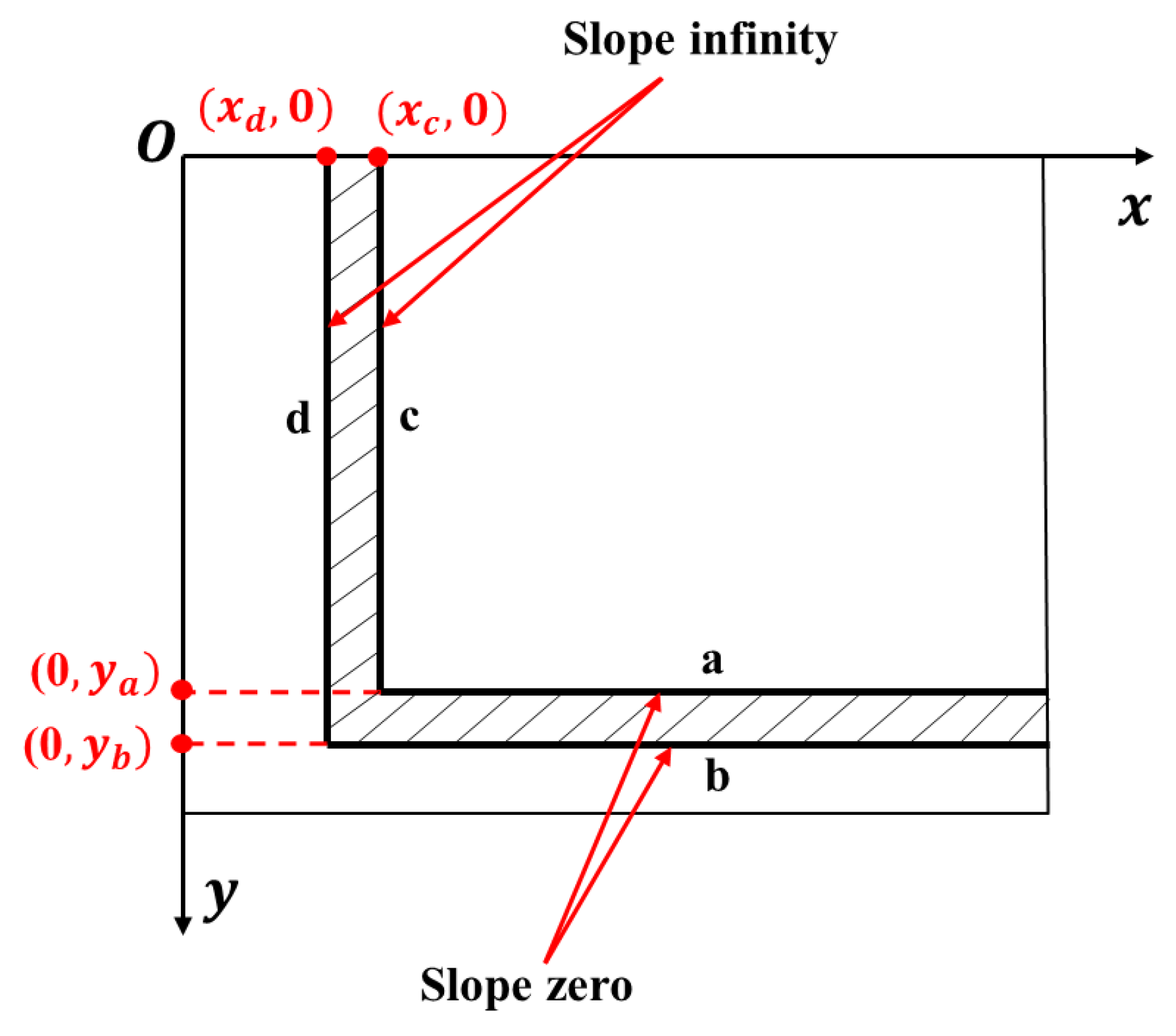
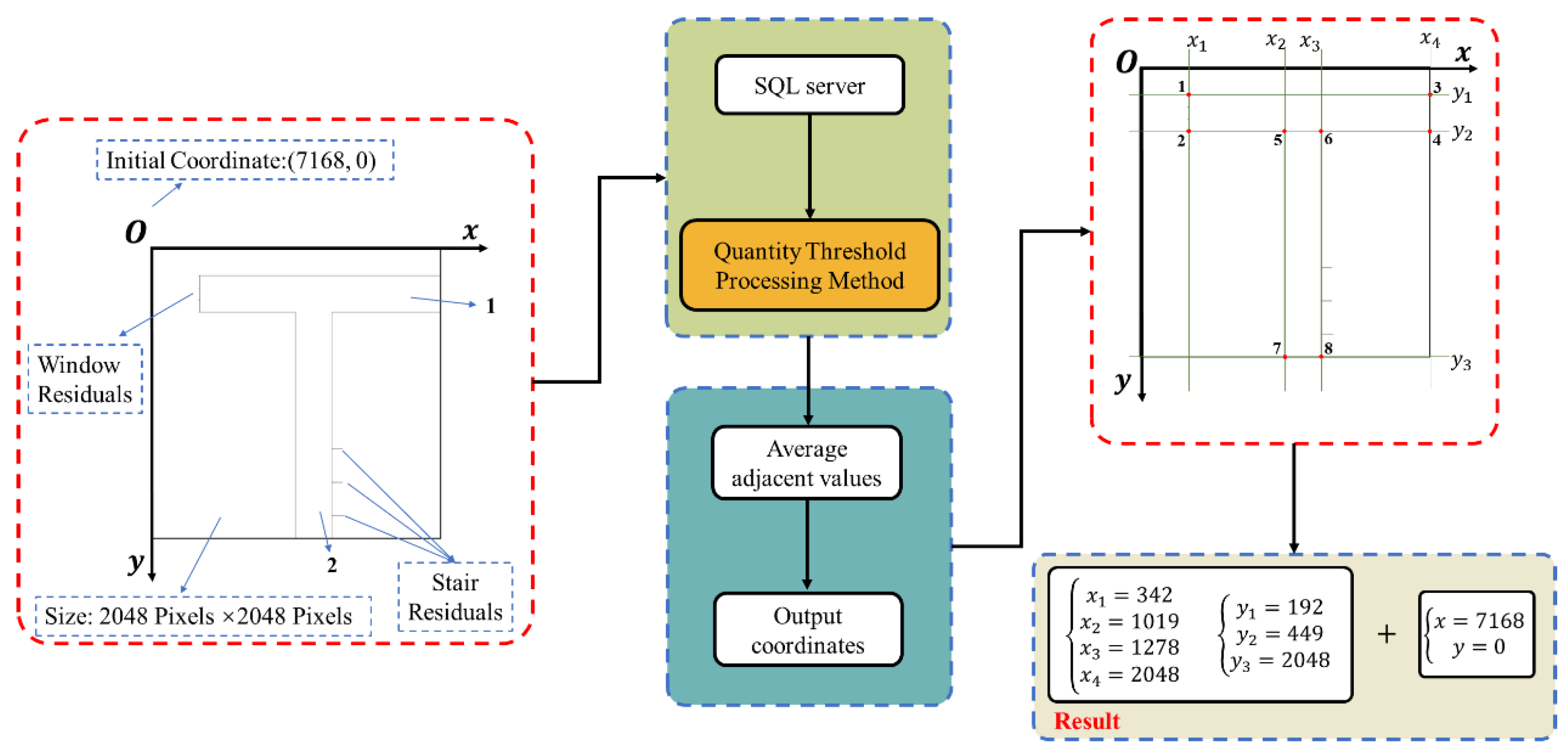
In Cartesian coordinates, line detection addresses slopes of zero, infinite, or nonzero values. This study introduces the “Quantity Threshold Processing Method,” applied to parallel lines with zero or infinite slopes, using a pixel count threshold. As illustrated in Figure 11, the Y coordinates for one-pixel-wide line segments a and b are queried. When these segments are aligned parallel to the X-axis, points along a given Y value are collectively assessed. Exceeding the threshold triggers the output of the and values. The method then retrieves the extreme X coordinates for these Y values and calculates the wall endpoints as their average. The wall width is derived from the Y interval, adjusted by a conversion ratio. This process efficiently defines the endpoints and width for walls indicated by segments a and b, thereby optimizing Cartesian line analysis.
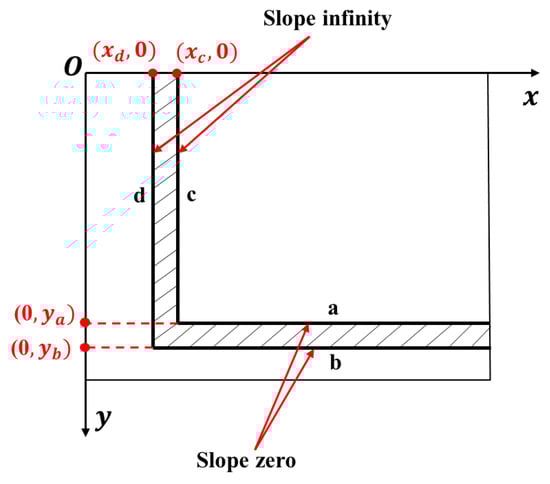
Figure 11.
Illustrative diagram of line segments exhibiting zero or infinite slope.
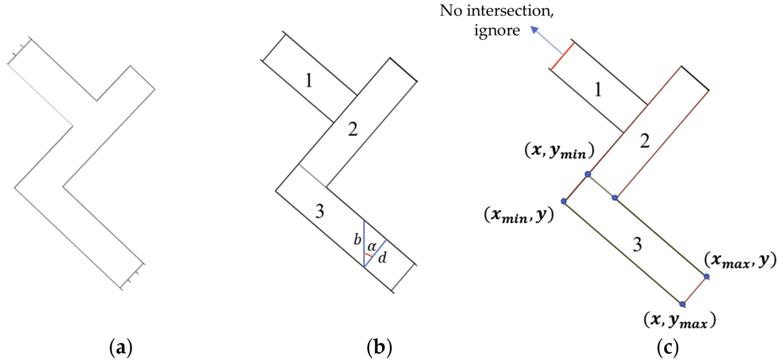
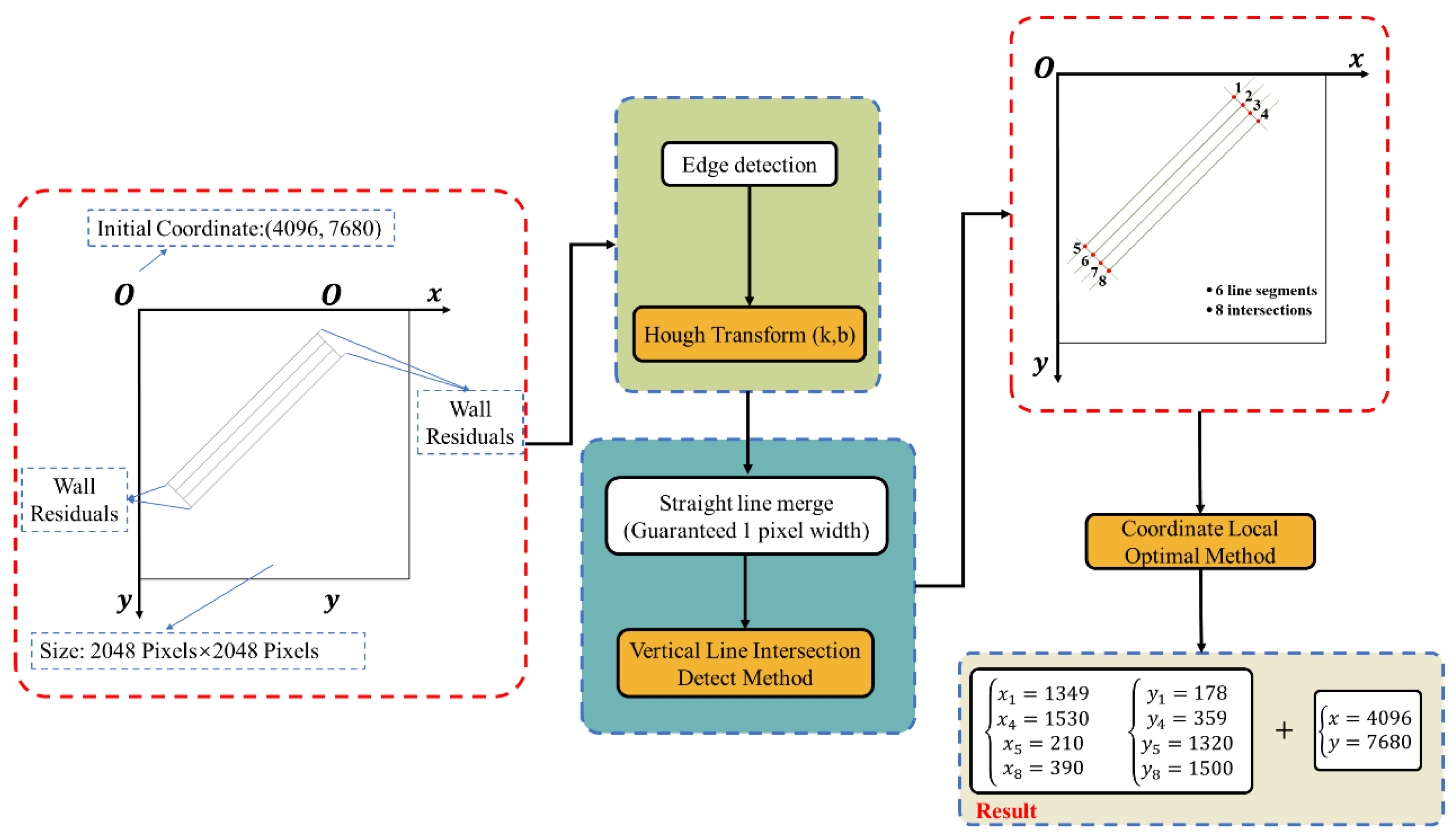
For lines with nonzero and non-infinite slopes, intersection points are computed, and essential coordinates are isolated. The Probabilistic Hough Line Detection method, using SQL Server queries, identifies endpoints of these line segments based on their slopes and intercepts. This method, inapplicable to the “Quantity Threshold Processing Method,” necessitates an alternative for identifying intersections of vertical lines. As depicted in Figure 12, a wall with varied directional surfaces, including windows, is segmented by the Probabilistic Hough approach. When analyzing walls such as Wall 1 and Wall 3, managing parallel lines is crucial. Trigonometry determines wall width from the difference in intercepts, as shown in Figure 12b. Segments fall into a group if their intercept variances lie within two predetermined thresholds, calculated by the following designated formula:
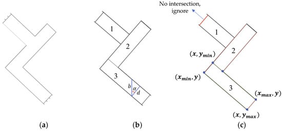
Figure 12.
Illustrative diagram of component coordinates derived from line segments with constant slope detection: (a) Three walls with residual profiles and windows; (b) Target blocking and parameter definition; (c) Coordinate detection.
In the formula, denotes the minimum threshold value and the maximum. Line segments with intercept differences that reside within these bounds are grouped together.
The study introduces the ‘Coordinate Local Extremum Method’ for pinpointing critical coordinates of structural elements with consistent slopes, like walls and stairs. For such elements, one of the key coordinates (X or Y) is invariably the extremum among the component’s vertices. This principle is delineated as follows:
“The ‘Vertical Line Intersection Detection Method,’ as shown in Figure 12c, extracts Wall 3’s coordinates. Trend lines, running parallel to the component’s projected direction, and intersecting perpendicular vertical lines are considered. Segments not intersecting with trend lines, such as Wall 1’s left segment, are excluded. The method discerns the wall’s vertices at five intersection points using the ‘Coordinate Local Extremum Method’. Endpoints are computed as the mean of adjacent intersections. The width of the wall is derived from the trigonometric relation of the trend lines’ intercept differences and the angle, detailed in Figure 12b, according to the following stated formula:
In the aforementioned formulas, α is the angle of inclination for Wall 3’s line segments, and and correspond to the intercepts of these segments, respectively. denotes the pixel width of the wall, and the actual width is calculated by multiplying d by a conversion ratio.
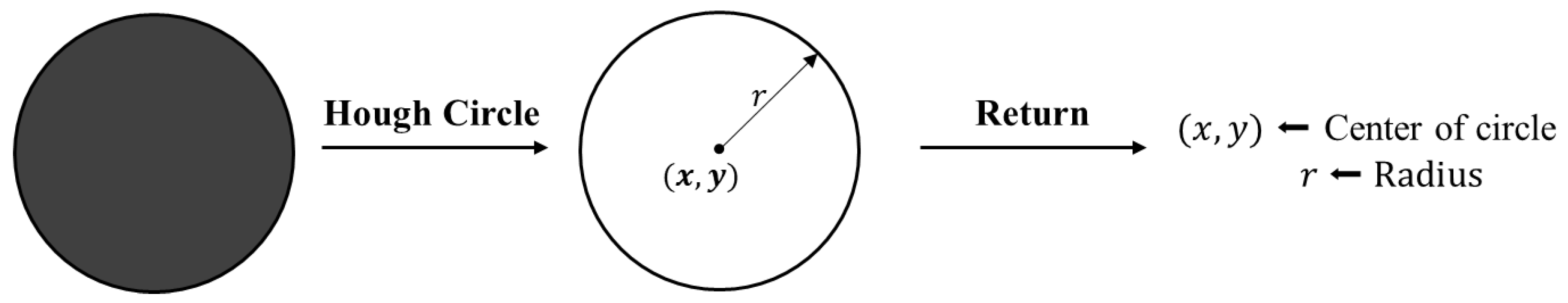
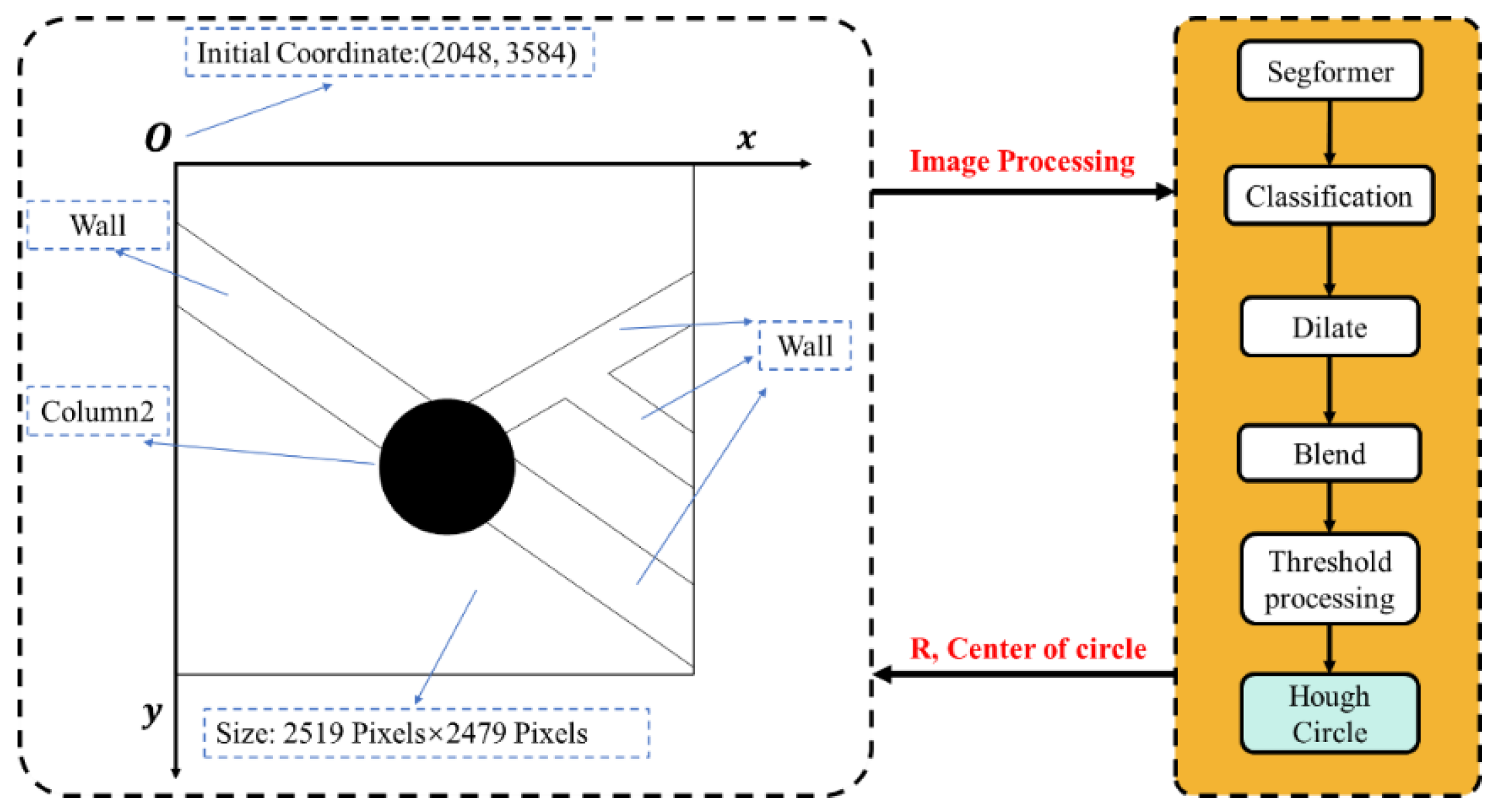
In circular analyses, Figure 13 illustrates a streamlined SQL query. The Hough Circle Detection algorithm detects circular perimeters, outputting central coordinates and radii. These parameters, stored on an SQL server, are retrievable through optimized queries. Multiplication of these results by a conversion factor yields the cylinder’s exact position and radius.
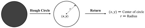
Figure 13.
Illustrative diagram of applying the Hough Circle Detection method for circular contour detection.
In the coordinate detection approach, line segments wider than a pixel, as shown in Figure 14, yield numerous intersections. For n-pixel-wide segments, up to intersections may result, hindering precise coordinate identification. To resolve this, an averaging process replaces these segments with single-pixel counterparts. Segments closer than a set threshold and with similar slopes are combined, their extremities averaged, thereby reducing segment width to one pixel and optimizing coordinate extraction.
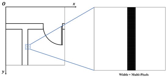
Figure 14.
Representation of pixel width of line segments in two-dimensional blueprints.
In conclusion, combining Hough Transform with SQL server improves image-based line segment coordinate detection’s efficiency and precision and extends its use.
3. Experiments
3.1. Experimental Environment
Semantic segmentation, image processing, and coordinate extraction were performed using an Intel Core i7-12700K processor (Intel Corporation, Santa Clara, CA, USA), 128 GB RAM (Kingston Technology Company, Inc., Fountain Valley, CA, USA), and Nvidia GeForce RTX 3090 GPU (Nvidia Corporation, Santa Clara, CA, USA). The SegFormer network was developed with the PyTorch-GPU, a specialized deep learning framework. SQL Server databases were deployed on Windows for efficient data management.
3.2. Characteristics and Partitioning of the Data Set
A comprehensive data set with annotated images is critical for training an effective semantic segmentation model. Due to the limited availability of open-source data, a specialized data set was compiled from Shanghai residential building blueprints, complying with national standards and classified into architectural and structural types. The network processes images at a resolution of 512 × 512 pixels, with the data divided into training, validation, and test sets at an 8:1:1 ratio. Training, validation, and testing facilitate model development, hyperparameter optimization, and performance evaluation, respectively. The data set includes varied categories to ascertain the model’s recognition accuracy:
- Independent Single-Target (13%): Isolated entities such as columns and walls;
- Single-Target Intersecting (8%): Overlapping elements of a single category, e.g., intersecting beams;
- Double-Target Intersecting (51%): Common combinations like walls with doors or columns;
- Multi-Target Connected (28%): Complex intersections involving multiple component types, such as walls with doors and windows.
3.3. Characteristics and Partitioning of the Data Set
The confusion matrix, composed of True Positives (TP), True Negatives (TN), False Positives (FP), and False Negatives (FN), quantifies the model’s test set accuracy, as detailed in Figure 15. In semantic segmentation, pixels are treated as discrete data points for classification.
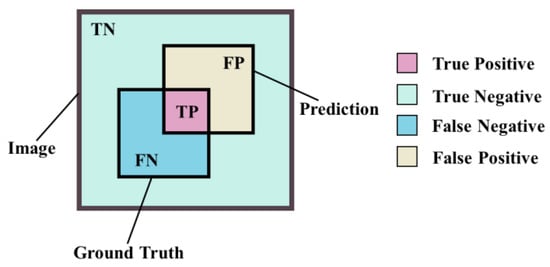
Figure 15.
Illustrative diagram showcasing the interrelationships of the four elements within a confusion matrix.
The confusion matrix facilitates the derivation of metrics to evaluate semantic segmentation performance, specifically Mean Intersection over Union (MIoU) and Pixel Accuracy (PA), whose formulas are provided:
In the formulas presented, represents the count of pixel classification categories. MIoU gauges semantic segmentation efficacy by averaging the IoU for all categories, comparing the overlap of predicted and ground truth labels per category. The cumulative mean of these comparisons yields an image’s MIoU. PA evaluates the correct pixel correspondences between predictions and ground truth.
3.4. Hyperparameter Settings
The SegFormer model’s performance is contingent on hyperparameters: learning rate, batch size, optimizer, pre-trained weights, learning rate decay, weight decay, loss function, and epoch count. Optimal configurations, identified through comparative analysis, are detailed in Table 3.
Table 3.
Configuration of hyperparameters for deep learning training.
3.5. Drawing Selection and Coordinate Detection
Detection is categorized into two approaches based on the contour line’s slope. One approach uses the raw image, the other the enlarged and rotation-filled image. It is established that one millimeter translates to 1.076 pixels in the raw image.
3.5.1. Components Composed of Line Segments with Zero or Infinite Slope
The ‘Quantity Threshold Processing Method’ is applied to analyze components. Figure 16, from a Shanghai villa’s blueprint, is the detection experiment subject. The blueprint includes line segments with horizontal or vertical orientations, representing essential architectural features like walls and openings. The case study focuses on detecting wall coordinates in a specific section, where the wall’s width is 240 mm, which is equivalent to 258.24 pixels.
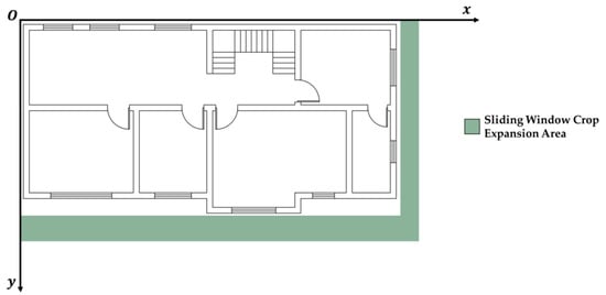
Figure 16.
Confirmation image of components constituted by line segments exhibiting zero or infinite slope.
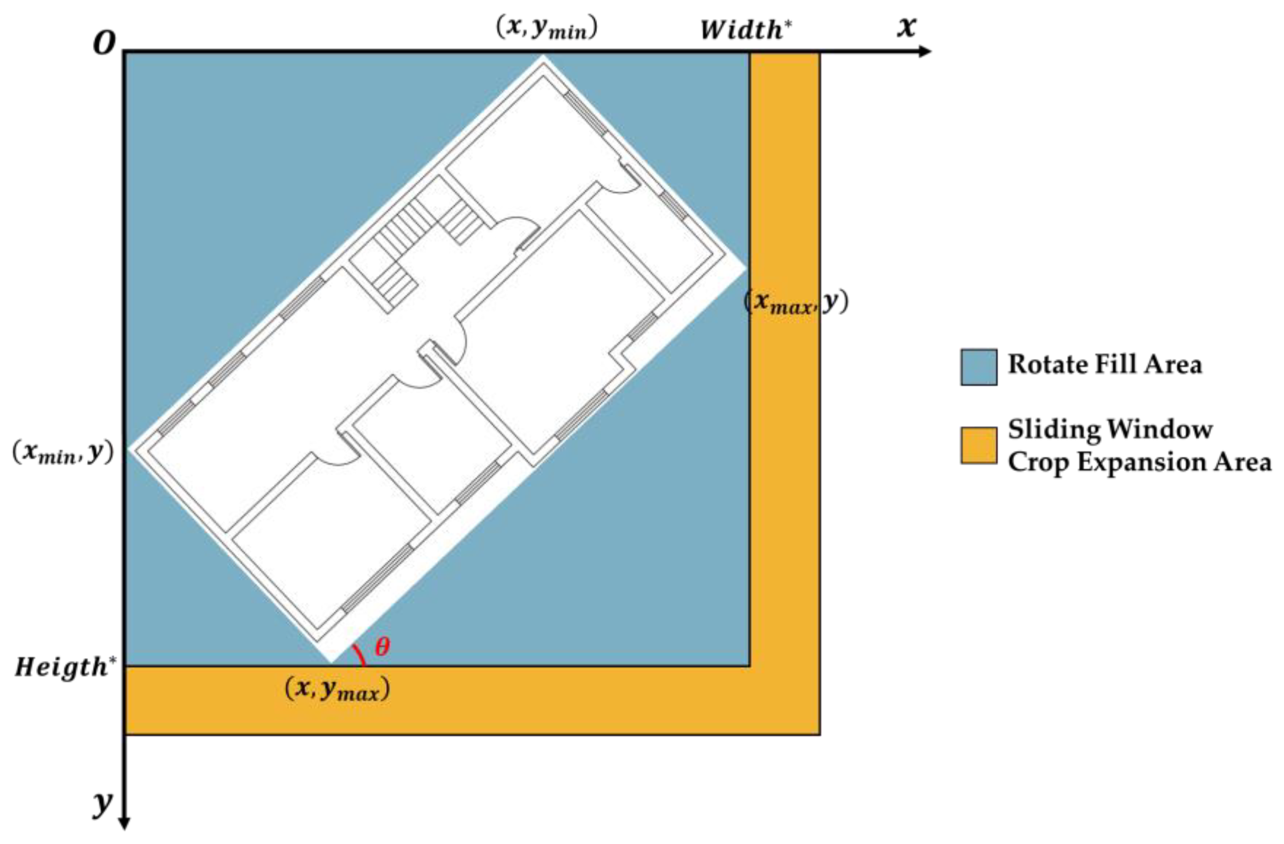
3.5.2. Components Composed of Line Segments with Constant Slope
The ‘Coordinate Local Maximum Method’ and ‘Vertical Line Intersection Detection Method’ are applied to these components. Figure 17 illustrates the original image rotated counterclockwise by a θ angle (0° < θ < 90°), here 45°, rendering line segment slopes uniform at 1 or −1. Image corners post-rotation are filled (blue) and expanded (orange), utilizing the remainder method from Figure 6 to streamline image segmentation and coordinate detection. The processing complies with the subsequent formula:

Figure 17.
Confirmation image of components constituted by line segments exhibiting constant slope.
In the aforementioned formulas, and denote the pixel dimensions post-rotation, whereas Width and Height refer to the dimensions of the expanded image. The term ‘mod’ signifies the modulus operation.
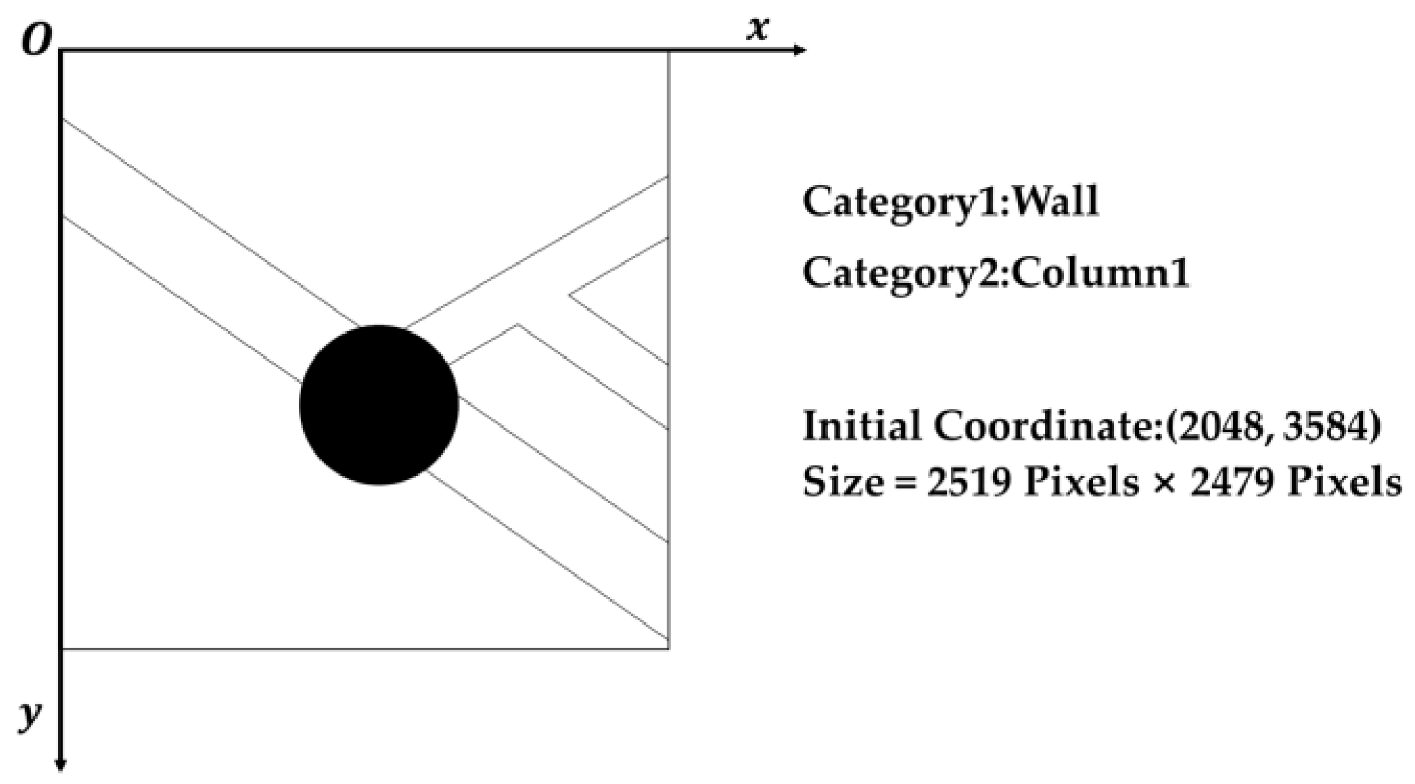
3.5.3. Circular Components
The investigation focuses on coordinate detection for circular elements in a Shanghai school’s architectural drawing. Figure 18 shows the initial layout, component intersections, and dimensions, with a conversion scale of 1 mm to 1.105 pixels.
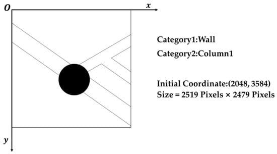
Figure 18.
Confirmation image and parameters illustrating the efficacy of circular component coordinate detection.
4. Results and Discussion
4.1. Performance Analysis of Deep Learning
4.1.1. Comparison of Deep Learning Models
The study assesses SegFormer against established semantic segmentation networks: PSPNet, U-Net, Deeplabv3+, and HRNet, underscoring SegFormer’s superior performance. Network descriptions consider baseline functionality using default backbones as detailed in Table 4. Models maintain original architecture, standard hyperparameters, and consistent data sets in training evaluations.
Table 4.
Selection matrix for backbone networks across different deep learning architectures.
Semantic segmentation models are trained on a consistent architectural data set and tested with a corresponding set of architectural images. Results are tabulated in Table 5.
Table 5.
Comparative performance of custom data set across various network architectures.
Using 200 training iterations, SegFormer demonstrates superiority in MIoU and PA metrics due to its effective encoder-decoder configuration and complex feature extraction network. With the exception of PSPNet, all models achieve over 90% MIoU and 95% PA, attesting to the custom data set’s quality and uniformity. Despite SegFormer’s longer training duration, this aspect is not critical to the study. The overall assessment validates the choice of SegFormer, suggesting that advanced feature extraction networks, despite increasing training times, improve performance.
4.1.2. Training Monitoring Analysis with Established Hyperparameter Configuration
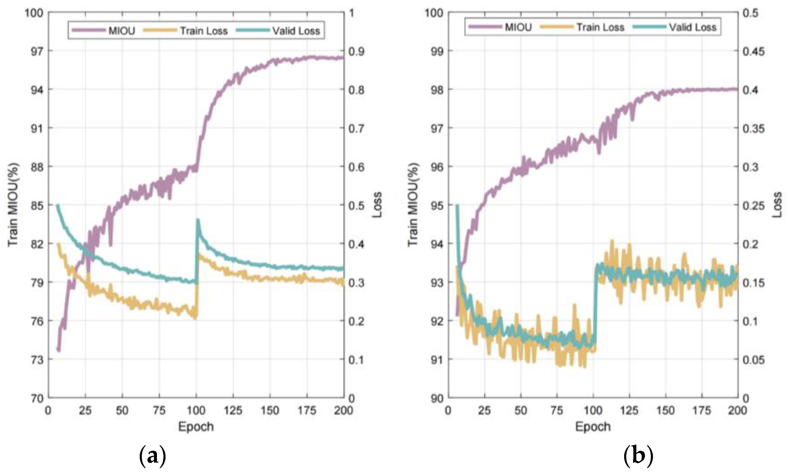
Figure 19 presents the variation in MIoU and Loss for two specialized drawing data sets under consistent network settings and hyperparameters. Training incorporates an initial 100-epoch phase with frozen layer weights, followed by 100 epochs with active weight adjustment. Owing to the expansive, high-quality data set, the network achieves a substantial MIoU within roughly five epochs and continues to improve until it stabilizes. Loss for both data sets converges quickly during the initial frozen phase. Subsequent weight unfreezing accelerates MIoU gains due to varying update velocities. Loss discrepancies between data sets are pronounced, with simplified category counts linked to reduced classification and detection errors. Loss peaks temporarily at the 100-epoch threshold as layers adapt to new data distributions and parameter settings. Training progression sees these layers recalibrate, with normalization stabilizing values and leading to a reduction and stabilization of Loss.
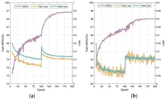
Figure 19.
Documenting the key metric variations throughout the model training process: (a) Architecture; (b) Structure.
Table 6 reports the model’s performance on the test set, with MIoU and PA exceeding 96% and 98%, respectively, denoting high accuracy. The superior results from professional data sets, despite their smaller size relative to architectural ones, are attributed to their lower component diversity. This simplicity allows for more focused learning on specific category features and reduces the incidence of classification errors.
Table 6.
Comparative performance of the SegFormer network across diverse domain-Specific data sets.
4.1.3. Training Monitoring Analysis with Established Hyperparameter Configuration
Table 7 and Table 8 reveal low misclassification rates among identified categories, with ‘BG’ representing the background and ‘A’ to ‘M’ corresponding to the component types from Figure 3 and Figure 4. Minor alignment issues in semantic segmentation, due to occasional component-background misclassifications, are acceptable given the task’s complexity, category diversity, and the applied contour dilation in subsequent processing.
Table 7.
Outcome of the confusion matrix from model training within the structural domain.
Table 8.
Outcome of the confusion matrix from model training within the architectural domain.
Table 7 and Table 8 indicate that components with simple linear designs are more prone to misclassification, with beams often mistaken for columns and walls for other categories due to their basic line structures. These patterns highlight the challenges of classifying simple contours and the importance of using large, augmented data sets for effective training.
4.2. Conclusions and Analysis of Component Coordinate Detection
4.2.1. Detection of Component Coordinates with Segments Formed by Slopes of Zero or Infinity
Figure 20 shows a 2048 px × 2048 px image obtained through sliding window cropping, with an origin at (7168, 0) in the global coordinate system. To map line coordinates from this image to the full image, add the origin coordinates to each localized coordinate set.
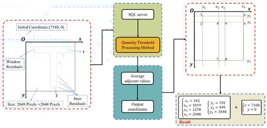
Figure 20.
Example of component coordinate detection constituted by line segments exhibiting zero or infinite slope.
Table 9 displays keypoint detection outcomes in terms of pixel, distance, and actual coordinates for two orthogonal walls, allowing for error assessment through distance comparison. Wall 1 runs parallel to the X-axis and Wall 2 to the Y-axis.
Table 9.
Analytical review of coordinate detection in components comprising line segments with zero or infinite slope.
Detection errors for wall keypoints remain below 0.05% on both the X and Y axes, impervious to distortion from unrelated component contours. These results satisfy practical application demands despite real-world challenges.
4.2.2. Coordinate Detection of Components with Segments Formed by Constant Slopes
The case study, using the detection method shown in Figure 17, presents a 2048 × 2048-pixel image in Figure 21, cropped using a sliding window technique with a starting point at (4096, 7680). Coordinates within this image require adjustment by this offset for accurate positioning.
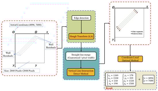
Figure 21.
Example of component coordinate detection constituted by line segments exhibiting constant slope.
Figure 21 identifies six window line segments and eight intersection points. The ‘Coordinate Local Extremum Method’ isolates the window’s four key points (1, 4, 5, 8) for comparison with true coordinates, detailed in Table 10.
Table 10.
Example of component coordinate detection constituted by line segments exhibiting constant slope.
Detection results show less than 0.06% error on the X and Y axes, demonstrating high precision. Unaltered by extraneous contours, these findings comply with practical precision standards.
4.2.3. Detection of Component Coordinates with Segments Formed by Slopes of Zero or Infinity
Figure 22 outlines a process for detecting coordinates to ascertain the image’s center of the circle (COC) and cylinder pixel radius.
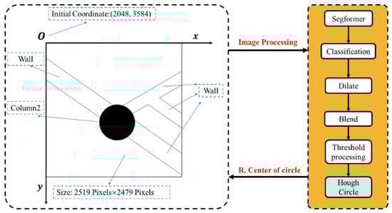
Figure 22.
Process for implementing circular component coordinate detection.
The detected pixel center coordinates and pixel radius, when multiplied by the conversion ratio and compared to actual values, yield the error margin listed in Table 11. These findings corroborate the precision of the Hough Circle Detection method, aligning with results from the line segment detection approach.
Table 11.
Evaluation and error analysis of detected circular components.
Detection methods incur errors primarily from three sources: rounding in representing actual distances in pixel coordinates, inaccuracies when pixel-to-distance conversion ratios are inexact, and precision loss in vector image transformations, such as scaling or rotation, due to interpolation.
4.3. Limitation
The presented method efficiently handles most coordinate detection cases, yet a few scenarios may present challenges.
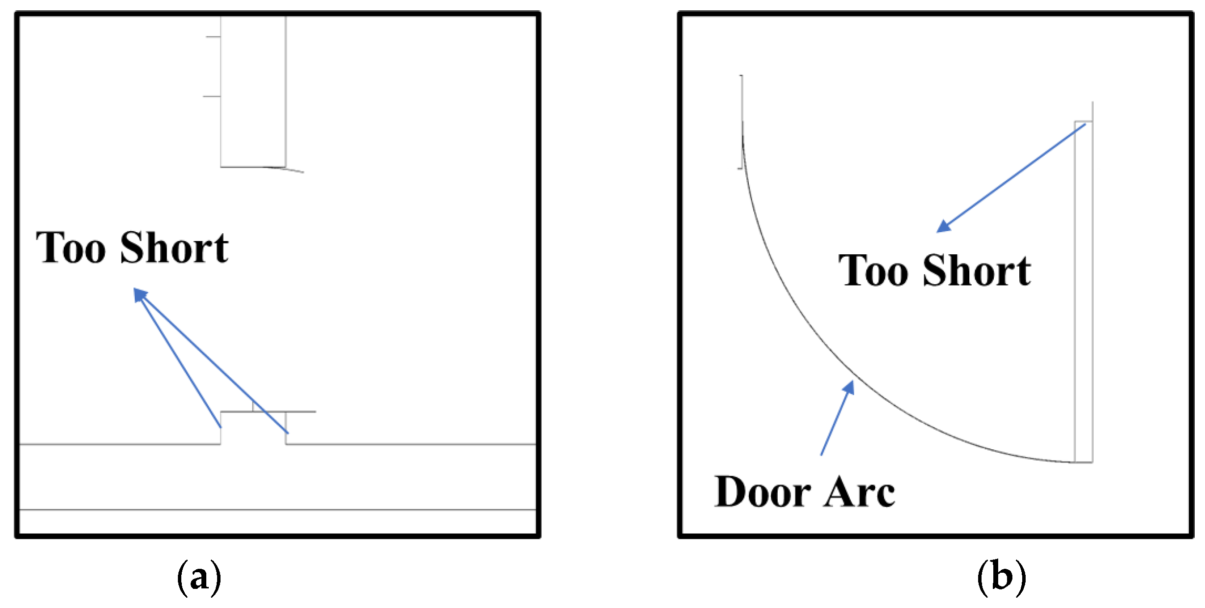
The inflation technique may resolve certain issues but has potential drawbacks in specific contexts. A standard inflation rate can lead to excessive expansion of some components, obscuring their contours. This effect is particularly marked when the component to be detected is shorter than surrounding non-target structures, increasing coordinate detection difficulty. Figure 23a shows that an ill-suited inflation ratio can disproportionately affect coordinate detection where shorter line segments, such as in a merlon’s wall, are overshadowed by the dominant contours of adjacent features like a door.
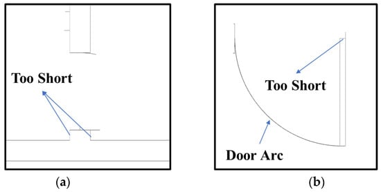
Figure 23.
Challenging examples encountered in applying coordinate detection algorithms: (a) Short wall; (b) Short line and arc.
In some instances, short key line segments may increase detection difficulties. As shown in Figure 23b, the door panel’s narrow key line segment, intersecting with the wall, could be problematic. A low detection threshold might identify this segment correctly but could also falsely detect multiple segments in the door arc. This could lead to the misidentification of the door arc as several minor segments with different slopes and intercepts in pixel images, reducing the accuracy of coordinate detection.
5. Conclusions
The study introduces a framework for recognizing components and pinpointing key coordinates in paper-based 2D blueprints, utilizing semantic segmentation and image processing. It examines the potential for accurate multi-category recognition and assesses the detection efficacy. Key findings include the following:
- The framework classifies components in two-dimensional blueprints using semantic data. Analyses include deep learning network selection, data set training, and error rates across categories. Notably, the ‘Edge Expansion Sliding Window Cropping Method’ was effective in high-resolution semantic segmentation, with the networks achieving IOU scores of 96.44% and 98.01%. Generally, prediction errors for component categories were below 0.5%, indicating standardized data sets and the precision and robustness of the models;
- By extracting semantic information, inflation and blending techniques effectively separate the target component’s contour in two-dimensional blueprints, minimizing irrelevant contour noise. Semantic segmentation’s classification properties refine coordinate detection on the processed blueprint, curtailing interference and errors;
- The integration of the “Quantity Threshold Processing Method” with SQL Server and algorithms such as the “Coordinate Local Extremum Method” and “Vertical Line Intersection Detection Method,” both incorporating the Hough Transform, yields improved coordinate detection accuracy. For line segment components, detection errors remain below 0.1%, and for circular components, within 0.15%, indicating exceptional performance.
This study initiates the exploration of coordinate recognition within two-dimensional blueprint components. Future work will aim to achieve the following:
- Employ higher-resolution blueprints to reduce coordinate detection errors by improving the pixel-to-dimension ratio;
- Enhance blueprint complexity and variety to broaden the study’s applicability;
- Refine coordinate detection techniques to address the identification of complex component contours;
- Leverage coordinate data to facilitate BIM model reconstruction and urban digitalization
With the progressive informatization of construction, deep learning is expected to become increasingly integral to the intelligent management and maintenance of structures.
Author Contributions
Conceptualization, S.G. and D.W.; methodology, S.G.; software, D.W.; validation, S.G.; formal analysis, S.G.; investigation, S.G.; resources, D.W.; data curation, S.G.; writing—original draft preparation, S.G.; writing—review and editing, D.W.; visualization, S.G.; supervision, D.W. All authors have read and agreed to the published version of the manuscript.
Funding
This research received no external funding.
Data Availability Statement
Data is available at https://drive.google.com/file/d/11c9GCrSOxAhGQhuM98SdNdASP165jR3T/view?usp=drive_link (accessed on 25 December 2023).
Conflicts of Interest
The authors declare no conflict of interest.
References
- Yang, B.; Liu, B.; Zhu, D.; Zhang, B.; Wang, Z.; Lei, K. Semiautomatic Structural BIM-Model Generation Methodology Using CAD Construction Drawings. J. Comput. Civ. Eng. 2020, 34, 04020006. [Google Scholar] [CrossRef]
- Volk, R.; Stengel, J.; Schultmann, F. Building Information Modeling (BIM) for existing buildings—Literature review and future needs. Autom. Constr. 2014, 38, 109–127. [Google Scholar] [CrossRef]
- Regassa Hunde, B. Debebe Woldeyohannes A. Future prospects of computer-aided design (CAD)—A review from the perspective of artificial intelligence (AI), extended reality, and 3D printing. Results Eng. 2022, 14, 100478. [Google Scholar] [CrossRef]
- Baduge, S.K.; Thilakarathna, S.; Perera, J.S.; Arashpour, M.; Sharafi, P.; Teodosio, B.; Shringi, A.; Mendis, P. Artificial intelligence and smart vision for building and construction 4.0: Machine and deep learning methods and applications. Autom. Constr. 2022, 141, 104440. [Google Scholar] [CrossRef]
- Wang, T.; Gan VJ, L. Automated joint 3D reconstruction and visual inspection for buildings using computer vision and transfer learning. Autom. Constr. 2023, 149, 104810. [Google Scholar] [CrossRef]
- Liu, F.; Wang, L. UNet-based model for crack detection integrating visual explanations. Constr. Build. Mater. 2022, 322, 126265. [Google Scholar] [CrossRef]
- Phan, D.T.; Ta, Q.B.; Huynh, T.C.; Vo, T.H.; Nguyen, C.H.; Park, S.; Choi, J.; Oh, J. A smart LED therapy device with an automatic facial acne vulgaris diagnosis based on deep learning and internet of things application. Comput. Biol. Med. 2021, 136, 104610. Available online: https://www.ncbi.nlm.nih.gov/pubmed/34274598 (accessed on 29 November 2023). [CrossRef]
- Phan, D.T.; Ta, Q.B.; Ly, C.D.; Nguyen, C.H.; Park, S.; Choi, J.; O Se, H.; Oh, J. Smart Low Level Laser Therapy System for Automatic Facial Dermatological Disorder Diagnosis. IEEE J. Biomed. Health Inform. 2023, 27, 1546–1557. Available online: https://www.ncbi.nlm.nih.gov/pubmed/37021858 (accessed on 24 November 2023). [CrossRef]
- Xia, Z.; Ma, K.; Cheng, S.; Blackburn, T.; Peng, Z.; Zhu, K.; Zhang, W.; Xiao, D.; Knowles, A.J.; Arcucci, R. Accurate identification and measurement of the precipitate area by two-stage deep neural networks in novel chromium-based alloys. Phys. Chem. Chem. Phys. 2023, 25, 15970–15987. Available online: https://www.ncbi.nlm.nih.gov/pubmed/37265373 (accessed on 26 November 2023). [CrossRef]
- Mo, Y.; Wu, Y.; Yang, X.; Liu, F.; Liao, Y. Review the state-of-the-art technologies of semantic segmentation based on deep learning. Neurocomputing 2022, 493, 626–646. [Google Scholar] [CrossRef]
- Shelhamer, E.; Long, J.; Darrell, T. Darrell, Fully convolutional networks for semantic segmentation. IEEE Trans. Pattern Anal. Mach. Intell. 2017, 39, 640–651. [Google Scholar] [CrossRef] [PubMed]
- Zhao, H.; Shi, J.; Qi, X.; Wang, X.; Jia, J. Pyramid scene parsing network. In Proceedings of the 2017 IEEE Conference on Computer Vision and Pattern Recognition (CVPR), Honolulu, HI, USA, 21–26 July 2017; pp. 6230–6239. [Google Scholar] [CrossRef]
- Ronneberger, O.; Fischer, P.; Brox, T. U-net: Convolutional networks for biomedical image segmentation. In Proceedings of the 2015 International Conference on Medical Image Computing and Computer-Assisted Intervention (MICCAI), Munich, Germany, 5–9 October 2015; Springer: Berlin/Heidelberg, Germany, 2015; pp. 234–241. [Google Scholar] [CrossRef]
- Vijay Badrinarayanan, R.C. Alex Kendall, Segnet: A deep convolutional encoder-decoder architecture for image segmentation. IEEE Trans. Pattern Anal. Mach. Intell. 2017, 39, 2481–2495. [Google Scholar] [CrossRef]
- Chen, L.; Papandreou, G.; Kokkinos, I.; Murphy, K.; Yuille, A. Semantic image segmentation with deep convolutional nets and fully connected crfs. arXiv 2014, arXiv:1412.7062v4. [Google Scholar]
- Chen, L.; Zhu, Y.; Papandreou, G.; Schroff, F.; Adam, H. Encoder-decoder with atrous separable convolution for semantic image segmentation. In Proceedings of the 2018 European Conference on Computer Vision (ECCV), Munich, Germany, 8–14 September 2018; Springer: Berlin/Heidelberg, Germany, 2018; pp. 833–851. [Google Scholar] [CrossRef]
- Vaswani, A.; Shazeer, N.; Parmar, N.; Uszkoreit, J.; Jones, L.; Gomez, A.N.; Kaiser, L.; Polosukhin, I. Attention is all you need. Adv. Neural Inf. Process. Syst. 2017, 30. [Google Scholar] [CrossRef]
- Xie, E.; Wang, W.; Yu, Z.; Anandkumar, A.; Alvarez, J.M.; Luo, P. SegFormer: Simple and efficient design for semantic segmentation with transformers. Adv. Neural Inf. Process. Syst. 2021, 34, 12077–12090. [Google Scholar]
- Dang, L.M.; Wang, H.; Li, Y.; Nguyen, L.Q.; Nguyen, T.N.; Song, H.K.; Moon, H. Deep learning-based masonry crack segmentation and real-life crack length measurement. Constr. Build. Mater. 2022, 359, 129438. [Google Scholar] [CrossRef]
- Yuan, Y.; Zhang, N.; Han, C.; Liang, D. Automated identification of fissure trace in mining roadway via deep learning. J. Rock Mech. Geotech. Eng. 2023, 15, 2039–2052. [Google Scholar] [CrossRef]
- Zhou, Q.; Situ, Z.; Teng, S.; Liu, H.; Chen, W.; Chen, G. Automatic sewer defect detection and severity quantification based on pixel-level semantic segmentation. Tunn. Undergr. Space Technol. 2022, 123, 104403. [Google Scholar] [CrossRef]
- Ji, A.; Xue, X.; Wang, Y.; Luo, X.; Xue, W. An integrated approach to automatic pixel-level crack detection and quantification of asphalt pavement. Autom. Constr. 2020, 114, 103176. [Google Scholar] [CrossRef]
- Ramani, V.; Zhang, L.; Kuang, K.S.C. Probabilistic assessment of time to cracking of concrete cover due to corrosion using semantic segmentation of imaging probe sensor data. Autom. Constr. 2021, 132, 103963. [Google Scholar] [CrossRef]
- Wang, H.; Li, Y.; Dang, L.M.; Lee, S.; Moon, H. Pixel-level tunnel crack segmentation using a weakly supervised annotation approach. Comput. Ind. 2021, 133, 103545. [Google Scholar] [CrossRef]
- Hao, Z.; Lu, C.; Li, Z. Highly accurate and automatic semantic segmentation of multiple cracks in engineered cementitious composites (ECC) under dual pre-modification deep-learning strategy. Cem. Concr. Res. 2023, 165, 107066. [Google Scholar] [CrossRef]
- Shim, J.-H.; Yu, H.; Kong, K.; Kang, S.-J. FeedFormer: Revisiting Transformer Decoder for Efficient Semantic Segmentation. Proc. AAAI Conf. Artif. Intell. 2023, 37, 2263–2271. [Google Scholar] [CrossRef]
- Meeran, S.; Pratt, M.J. Automated feature recognition from 2D drawings. Comput.-Aided Des. 1993, 25, 7–17. [Google Scholar] [CrossRef]
- Meeran, S.; Taib, J.M. A generic approach to recognising isolated, nested and interacting features from 2D drawings. Comput.-Aided Des. 1999, 31, 891–910. [Google Scholar] [CrossRef]
- Hwang, H.-J.; Han, S.; Kim, Y.-D. Recognition of design symbols from midship drawings. Ocean. Eng. 2005, 32, 1968–1981. [Google Scholar] [CrossRef]
- Huang, H.C.; Lo, S.M.; Zhi, G.S.; Yuen, R.K.K. Graph theory-based approach for automatic recognition of CAD data. Eng. Appl. Artif. Intell. 2008, 21, 1073–1079. [Google Scholar] [CrossRef]
- Yin, M.; Tang, L.; Zhou, T.; Wen, Y.; Xu, R.; Deng, W. Automatic layer classification method-based elevation recognition in architectural drawings for reconstruction of 3D BIM models. Autom. Constr. 2020, 113, 103082. [Google Scholar] [CrossRef]
- Neb, A.; Briki, I.; Schoenhof, R. Development of a neural network to recognize standards and features from 3D CAD models. Procedia CIRP 2020, 93, 1429–1434. [Google Scholar] [CrossRef]
- Manda, B.; Dhayarkar, S.; Mitheran, S.; Viekash, V.K.; Muthuganapathy, R. ‘CADSketchNet’—An Annotated Sketch dataset for 3D CAD Model Retrieval with Deep Neural Networks. Comput. Graph. 2021, 99, 100–113. [Google Scholar] [CrossRef]
- Zhao, Y.; Deng, X.; Lai, H. Reconstructing BIM from 2D structural drawings for existing buildings. Autom. Constr. 2021, 128, 103750. [Google Scholar] [CrossRef]
- Pan, Z.; Yu, Y.; Xiao, F.; Zhang, J. Recovering building information model from 2D drawings for mechanical, electrical and plumbing systems of ageing buildings. Autom. Constr. 2023, 152, 104914. [Google Scholar] [CrossRef]
- Liu, X.; Wu, Z.; Wang, X. Validity of non-local mean filter and novel denoising method. Virtual Real. Intell. Hardw. 2023, 5, 338–350. [Google Scholar] [CrossRef]
- Zheng, J.; Song, W.; Wu, Y.; Liu, F. Image interpolation with adaptive k-nearest neighbours search and random non-linear regression. IET Image Process. 2020, 14, 1539–1548. [Google Scholar] [CrossRef]
- Wilson, G.R. Morphological operations on crack coded binary images. IEE Proc.—Vis. Image Signal Process. 1996, 143, 171. [Google Scholar] [CrossRef]
- Chutatape, O.; Guo, L. A modified Hough transform for line detection and its performance. Pattern Recognit. 1999, 32, 181–192. [Google Scholar] [CrossRef]
- Yao, Z.; Yi, W. Curvature aided Hough transform for circle detection. Expert Syst. Appl. 2016, 51, 26–33. [Google Scholar] [CrossRef]


Disclaimer/Publisher’s Note: The statements, opinions and data contained in all publications are solely those of the individual author(s) and contributor(s) and not of MDPI and/or the editor(s). MDPI and/or the editor(s) disclaim responsibility for any injury to people or property resulting from any ideas, methods, instructions or products referred to in the content. |
© 2023 by the authors. Licensee MDPI, Basel, Switzerland. This article is an open access article distributed under the terms and conditions of the Creative Commons Attribution (CC BY) license (https://creativecommons.org/licenses/by/4.0/).