Hierarchical Graph Neural Network: A Lightweight Image Matching Model with Enhanced Message Passing of Local and Global Information in Hierarchical Graph Neural Networks

Abstract

Graph Neural Networks (GNNs) have gained popularity in image matching methods, proving useful for various computer vision tasks like Structure from Motion (SfM) and 3D reconstruction. A well-known example is SuperGlue. Lightweight variants, such as LightGlue, have been developed with a focus on stacking fewer GNN layers compared to SuperGlue. This paper proposes the h-GNN, a lightweight image matching model, with improvements in the two processing modules, the GNN and matching modules. After image features are detected and described as keypoint nodes of a base graph, the GNN module, which primarily aims at increasing the h-GNN’s depth, creates successive hierarchies of compressed-size graphs from the base graph through a clustering technique termed SC+PCA. SC+PCA combines Principal Component Analysis (PCA) with Spectral Clustering (SC) to enrich nodes with local and global information during graph clustering. A dual non-contrastive clustering loss is used to optimize graph clustering. Additionally, four message-passing mechanisms have been proposed to only update node representations within a graph cluster at the same hierarchical level or to update node representations across graph clusters at different hierarchical levels. The matching module performs iterative pairwise matching on the enriched node representations to obtain a scoring matrix. This matrix comprises scores indicating potential correct matches between the image keypoint nodes. The score matrix is refined with a ‘dustbin’ to further suppress unmatched features. There is a reprojection loss used to optimize keypoint match positions. The Sinkhorn algorithm generates a final partial assignment from the refined score matrix. Experimental results demonstrate the performance of the proposed h-GNN against competing state-of-the-art (SOTA) GNN-based methods on several image matching tasks under homography, estimation, indoor and outdoor camera pose estimation, and 3D reconstruction on multiple datasets. Experiments also demonstrate improved computational memory and runtime, approximately 38.1% and 26.14% lower than SuperGlue, and an average of about 6.8% and 7.1% lower than LightGlue. Future research will explore the effects of integrating more recent simplicial message-passing mechanisms, which concurrently update both node and edge representations, into our proposed model.

1. Introduction

Image matching involves finding correspondences between key features extracted from pairs of similar images. This process is beneficial for tasks like homography [1,2,3,4,5] and camera pose estimation [6]. These tasks, in turn, are useful for various computer vision applications, such as Structure from Motion (SfM) [7], 3D reconstruction [4], Simultaneous Localization and Mapping (SLAM) [8], change detection [9], etc. Image matching is also used in various real-world applications, like logo spotting [10], person re-identification [11], UAV visual navigation [12], medical image registration [9,13], etc. The conventional image matching pipeline typically involves three main steps: (1) feature detection and description, (2) feature matching, and (3) geometric transformation estimation. This paper concentrates mainly on the feature matching step. Modern feature matching techniques utilize Graph Neural Networks (GNNs) [2,3,4,13,14]. In GNNs, image keypoints are represented as nodes, and their relationships are represented as edges in graphs [13,15,16]. A popular GNN-based feature matching technique is SuperGlue [2], which ranked highly in the CVPR 2020 workshop. SuperGlue [2] has been extensively studied, leading to variants like LightGlue [3], LifelongGlue [4], AdaSG [8], etc.

From a high-level perspective, these variants either decrease or increase the number of GNN layers, denoted as $L$. Decreasing $L$ can make the model more scalable for devices with limited resources by reducing computational complexity. On the other hand, increasing $L$ can improve accuracy and support continual learning but comes at the cost of increased computational complexity. From a technical perspective, one fundamental motivation for adjusting (decreasing or increasing) $L$ is the message-passing mechanism of the graphs within the GNN. This mechanism iteratively passes information between adjacent keypoint nodes connected by edges. By standard, the mechanism predominantly captures local information surrounding each node [17], ensuring adjacent (neighbor) nodes with similar local structures learn comparable representations [18] from each other. This implies that, while the standard message-passing mechanism easily captures local information, it faces challenges in aggregating global information over a long range and struggles with interactions between non-adjacent nodes at a global level [19,20].

This inherent limitation constrains the expressivity of GNN models [21], restricting them from utilizing fixed locality information for computing node representations [22]. Consequently, relying solely on the standard message-passing mechanism for image matching tasks results in keypoints that are mostly limited to local information, leading to degraded performance [21,22]. Therefore, it is a promising research area to explore methods for GNN-based feature matching techniques capable of capturing both local and global information for optimal performance. Research in this area often relies on the fundamental strategy of increasing the number of message-passing iterations, denoted as $t$, by stacking $L$ [23,24]. A single round of message-passing iteration $t$ creates a single GNN layer $L$. In doing so, the matching model will still predominantly capture local information among nodes. To spread local information globally across multiple layers, increasing $t$ entails executing multiple rounds of the standard message-passing process for a sufficient number of iterations $t$. This process is analogous to stacking multiple GNN layers $L$, which, in turn, increases the depth of the graph network and expands the receptive field of each node [20].

A similar strategy was observed with SuperGlue [2], which stacks $L=9$ GNN layers. However, stacking $L$ layers to enable multiple message-passing for $t$ iterations can result in overly similar or indistinguishable node representations, commonly known as the over-smoothing problem [19,22,25]. Over-smoothing causes an exponential convergence of similarities among node features, which diminishes the GNN model’s discriminative power to capture nuanced differences between nodes in the graph. Consequently, GNN-based image matching models like SuperGlue [2], while efficient, may not benefit from increasing the number of layers in a single network depth beyond a certain threshold [20]. LifelongGlue [4] introduced a novel approach to address this challenge faced by SuperGlue [2] by increasing the number of layers in its GNN. In its attempt to enable multiple message-passing iterations and capture both local and global information, LifelongGlue [4] increases $L$ while implementing a continual learning strategy. Instead of utilizing a single network depth like SuperGlue [2], LifelongGlue [4] adopts two distinct networks: the memory model (MM) and the live model (LM) networks, each comprising $L=9$ stacked GNN layers. This setup allows for the flexibility of increasing the total network depth to 18 GNN layers. These two networks also have layer-wise connections to facilitate continuous message flow between them. However, this strategy leads to increased computation time during inference, resulting in quadratic time complexity $\mathrm{O}\left(n^2\right)$, where $n$ represents the number of keypoints [4]. Consequently, the matching layer’s runtime also increases as the number of keypoints increases.

Both SuperGlue [2] and LifelongGlue [4] clearly demand significant computational time and memory resources. This limitation restricts their training and makes their adoption impractical for numerous real-life applications, particularly on resource-constrained platforms like robots and mobile phones [3,8]. As a solution to the above limitations of SuperGlue [2] and LifelongGlue [4], a lightweight variant called LightGlue [3] has been proposed. LightGlue [3] aims to stack multiple GNN layers for multiple message-passing iterations, with the sole objective of capturing both local and global information. In contrast to SuperGlue [2] and LifelongGlue [4], LightGlue [3] achieves this goal by reducing the number of GNN layers.

LightGlue [3] achieves this by adaptively modulating the number of layers stacked deep within the graph network’s depth. It evaluates discriminative information (such as visual overlap, appearance, or similarity) in image pairs, decides whether predictions require further computations within the network depth, and stops at earlier layers if additional computations are unnecessary. Although LightGlue [3] also occasionally sets $L=9$ in experiments, it also reports instances where the network depth stops increasing at the third and eighth GNN layers for easier and more difficult matching tasks, respectively. Similarly, AdaSG [8], another lightweight variant, also adapts to the similarity of input image pairs.

Furthermore, LightGlue [3] and AdaSG [8] are lightweight variants primarily focused on discriminative information in image pairs, often more likely to revert to the settings where $L=9$ of GNN layers during the message passing of local and global information. For these reasons, this study proposes a lightweight GNN-based feature matching model with an enhanced message-passing mechanism to capture local and global information between image pairs. Inspired by the existing literature highlighting the categorization of clustering methods into local or global, based on the information they capture [26,27] and the notion that lightweight operation is required to evaluate graph clustering where a graph is compressed from its original graph [28,29,30], we propose that a lightweight GNN-based deep-feature matcher can benefit from clustering. We establish that compressing graphs through hierarchical levels for iterative message-passing processes can be analogous to stacking graph layers, as with the case of conventional ‘Glue’-based GNN feature matching models. Therefore, our proposed approach—enhancing the message-passing of global and local information within and across compressed graphs organized at multiple hierarchical levels of the network’s depth—does not aim to directly address the over-smoothing problem through layer stacking, as advocated by the aforementioned approaches. Instead, our focus lies in improving the distinguishability of learned node representations through graph clustering at various hierarchy levels.

We can observe at this point that the proposed approach has two main advantages over existing GNN models: (a) constructing hierarchical GNNs by successively stacking multiple more compressed-size graphs in levels; in each hierarchical level, a compressed graph is created from a clustering technique that preserves the local and global information of nodes and graphs. (b) Enhancing the standard message-passing procedure that, in itself, allows nodes to efficiently aggregate their local features within each node cluster and global features across the broader hierarchies of graphs. These provide a dual benefit to our proposed h-GNN by enabling it to achieve a double gain of local and global information.

Contribution

The contribution of this paper is three-fold:

• Propose a hybrid clustering method termed SC+PCA which integrates the objective function of Principal Component Analysis (PCA) with that of the Spectral Clustering model to preserve local and global information in graphs;
• Create a hierarchical GNN (h-GNN) by successively stacking multiple more compressed-size graphs in hierarchical levels as a means of increasing the network’s depth through SC+PCA;
• Propose message-passing mechanisms that inherently propagate local and global messages among nodes and across graphs in four ways: First, by maintaining the standard message propagation as local information within neighboring nodes. Second, by propagating messages as global information from nodes of graphs to nodes of another graph sequentially lower in the hierarchy of the graph network’s depth. Third, by propagating messages as global information from nodes of graphs to nodes of another graph sequentially higher in the hierarchy of the network’s depth. Fourth, by propagating messages as global information from nodes of the global graph in the highest hierarchy to nodes of the base graph in the lowest hierarchy of the network’s depth.

The remaining part of this paper is organized as follows: Section 2 presents the proposed h-GNN. The comparative evaluation findings derived from detailed experiments, along with discussions, are outlined in Section 3, and Section 4 concludes the paper and gives recommendations.

2. Proposed Hierarchical Graph Neural Network (h-GNN)

2.1. Overview of the Proposed Approach

This paper proposes the h-GNN, a feature matching model that employs message-passing mechanisms to facilitate the exchange of both local and global information between nodes of graphs at different levels of the network. The approach consists of two consecutive steps: (1) keypoint detection and description, and (2) feature matching. The keypoint detection and description step enriches keypoints with positional and visual cues. The feature matching step also has two modules, which are the GNN and the matching modules. Under the GNN module, three sub-steps are performed. First, an input base graph is created using the enriched keypoints as the graph’s nodes. Second, a clustering technique is applied to the base graph to generate a compressed graph at an initial hierarchical level. Subsequently, this clustering process is repeated on the consecutive compressed graphs multiple times, leading to the creation of graphs at successive hierarchical levels. Third, message-passing schemes facilitate information exchange among nodes within and across hierarchy levels. The detailed explanation regarding the next module, the matching module, will be deferred to Section 2.2.2. Figure 1 provides an overview of the proposed h-GNN framework, illustrating its steps, modules, and sub-steps.

2.2. Technical Details of the Proposed Approach

The subsequent paragraphs elaborate on the technical details of the general steps and subcomponents in Figure 1. Figure 2 illustrates the technical details of the architecture and workflow of the proposed hierarchical Graph Neural Network (h-GNN) model. Its core idea revolves around improving the exchange of local and global information among nodes and across hierarchical graphs through enhanced message passing.

2.2.1. Feature Detection and Description Step

The initial parts on the left side of Figure 2 provide a visual representation of this step. Given an image pair $\left(I^{\left(\mathrm{A}\right)},I^{\left(\mathrm{B}\right)}\right)$, keypoints $\left({\mathcal{K}}^{\left(\mathrm{A}\right)},{\mathcal{K}}^{\left(\mathrm{B}\right)}\right)$ are detected and processed to obtain their feature descriptors $\left({\mathcal{D}}^{\left(\mathrm{A}\right)},{\mathcal{D}}^{\left(\mathrm{B}\right)}\right)$. Next, the $\mathrm{k}\mathrm{E}\mathrm{n}\mathrm{c}$ encoder captures the positional information of keypoints for the image pair, as $\left(d_{\left(pos\right)}^{\left(\mathrm{A}\right)},d_{\left(pos\right)}^{\left(\mathrm{B}\right)}\right)$. Similarly, the d$\mathrm{E}\mathrm{n}\mathrm{c}$ encoder captures the visual information of descriptors, also for the image pair, as $\left(d_{\left(vis\right)}^{\left(\mathrm{A}\right)},d_{\left(vis\right)}^{\left(\mathrm{B}\right)}\right)$. Then, the keypoints and descriptors, enriched with positional and visual contextual cues derived from the image, are merged $\left(\oplus \right)$ to create the image keypoint features. These enriched image keypoints are a more distinct and informative representation of the image features. Following that, the feature matching step utilizes the enriched keypoint descriptors as nodes $v_i\in \mathcal{V}$ of the base graph $\mathcal{G}$.

2.2.2. Feature Matching Step

The feature matching step consists of two major modules, the GNN and the matching modules. The GNN module begins with defining the base graph from the enriched image keypoints. The first iteration of clustering is applied to this base graph to create the first hierarchical level of the compressed graph. Subsequent iterations of the clustering technique are then applied to generate successive hierarchical levels of compressed graphs. A dual non-contrastive clustering loss function is used to guide the clustering process and ensure clearer clustering of the graphs. The GNN module primarily aims at increasing h-GNN’s depth. Section 2.2.1 provides a comprehensive explanation of the procedures involved in the GNN module. The matching module performs iterative pairwise matching on the keypoint nodes to obtain a score matrix, which contains scores of all possible correct matches between the keypoints. The score matrix is refined with a ‘dustbin’ matrix to suppress outlier keypoints that do not have reliable matches. The Sinkhorn algorithm is used to generate a final partial assignment from the refined score matrix. There is a reprojection loss that facilitates the semi-supervised optimization of keypoint match positions. Further details about the matching module are covered in Section 2.2.2 of this paper. Details of the two loss functions used for each module are discussed in Section 2.2.3.

GNN Module

In this module of the h-GNN model, the process begins by defining the base graphs. These base graphs serve as the foundation for further processes. Subsequently, successive layers of compressed graphs are generated through a clustering technique. This iterative clustering technique is aimed at increasing the depth of the GNN by creating hierarchies of graphs.

Base Graph Definition: The structure of the base graph is defined in a manner similar to the initial graph structure of SuperGlue [2]. The set of nodes $\mathcal{V}=\left\{v_1,v_2,\dots ,v_n\right\}$ and edges $\mathcal{E}\subseteq \mathcal{V}\times \mathcal{V}$ are consequently defined for the base graph $\mathcal{G}=\left(\mathcal{V},\mathcal{E}\right)$ as follows. Use $n$ number of keypoints to represent nodes, then use the visual and position similarities between these keypoints to represent edges of the base graph $\mathcal{G}$. From Figure 3, it can be observed that the apparent input to the base graph $\mathcal{G}$ is the merged image keypoint features, i.e., $d_{\left(vis\right)}^{\left(*\right)}\oplus d_{\left(pos\right)}^{\left(*\right)}$ from the ‘feature detection and description step’. Additionally, we define two types of undirected edges, creating a multiplex structure for initial message passing. The first is the intra-image (self-) edges, which connect keypoints within the same image, and the second is the inter-image (cross-) edges, which connect keypoints from one image to those in the other. Later in this section, details on the self- and cross-attention mechanisms of keypoint connections are discussed.

Increasing h-GNN depth: Here, successive hierarchies of graphs are created through clustering, progressively increasing the network’s depth. This procedure is analogous to the stacking of $L$ multiple layers in other GNN-based feature matchers like SuperGlue [2]. Another essential objective achieved here is the preservation of both local and global information within nodes and across the entire graph. This preservation is achieved by organizing the graphs into multiple hierarchical levels of successively compressed mega-graphs at each iteration $l$ of the SC+PCA clustering technique. From this point onward, we give a concise mathematical description augmented with a figure illustration (see Figure 3), explaining how the network’s depth is increased.

Nodes $v_i\in \mathcal{V}$ of the base graph $\mathcal{G}$ can be progressively clustered into mega-node structures up to $L$ times, i.e., $L$ distinct hierarchical levels as follows: $\left\{{\mathcal{V}}_1^{\left(1\right)},{\mathcal{V}}_1^{\left(2\right)},\dots ,{\mathcal{V}}_1^{\left(L\right)},{\mathcal{V}}_2^{\left(1\right)},\dots ,{\mathcal{V}}_2^{\left(L\right)},{\mathcal{V}}_3^{\left(1\right)},\dots ,{\mathcal{V}}_i^{\left(L\right)}\right\}$. Within this structure, densely interconnected mega-nodes $v_i^{\left(l-1\right)}\in V_i^{\left(l-1\right)} \left(\mathrm{where} 1\le l\le L\right)$ of mega-graph ${\mathcal{G}}^{(l-1)}$ in the preceding hierarchical level $l-1$, are clustered into their corresponding mega-nodes $v_i^{\left(l\right)}\in V_i^{\left(l\right)}$ of the mega-graph ${\mathcal{G}}^{\left(l\right)}$ at the succeeding hierarchical level $l$.

Figure 3 illustrates this procedure of increasing the h-GNN depth. From Figure 3, we can observe that the nodes $\mathcal{V}$ of the base graph $\mathcal{G}$ are grouped into mega-nodes ${\mathcal{V}}_1^{\left(1\right)}$ of the mega-graph ${\mathcal{G}}^{\left(1\right)}$. Again, nodes within mega-graph ${\mathcal{G}}^{\left(1\right)}$ at hierarchical level $l=1$ are further grouped into mega-nodes ${\mathcal{V}}_2^{\left(1\right)}$ of the mega-graph ${\mathcal{G}}^{\left(2\right)}$ at hierarchical level $l+1=2$, and this progression continues iteratively until the global nodes $v_i^{\left(L\right)}\in V_i^{\left(L\right)}$ create the global graph ${\mathcal{G}}^{\left(L\right)}$. At each hierarchical level of clustering, our proposed SC+PCA clustering method is applied. The final iteration of this clustering technique results in the creation of the global graph ${\mathcal{G}}^{\left(L\right)}$. The global graph ${\mathcal{G}}^{\left(L\right)}$ is therefore the graph at the highest hierarchical level $L$. Again, later in this section, details on SC+PCA are discussed.

As the depth of the graph network increases, it is necessary to establish edges to facilitate message passing. This process simply involves creating edges between neighboring mega-nodes $v_i^{\left(l\right)}$ and $v_j^{\left(l\right)}$ in the mega-graph ${\mathcal{G}}^{\left(l\right)}$ if there are existing edges in the previous graph ${\mathcal{G}}^{(l-1)}$ connecting the mega-nodes. These edges facilitate the four types of message-passing mechanisms. The next section discusses the Spectral Clustering with the Principal Component Analysis (SC+PCA) method. After that section, the types of message-passing mechanisms are discussed.

• Spectral Clustering with Principal Component Analysis (SC+PCA)

The Spectral Clustering (SC) algorithm primarily focuses on preserving local information within nodes. However, when combined with Principal Component Analysis (PCA), the focus additionally includes preserving the global information of the entire graph. To clarify the process of SC+PCA, let us start by applying it to the base graph $\mathcal{G}$ to generate the corresponding mega-graph ${\mathcal{G}}^{\left(1\right)}$. In this application, the inputs to the SC+PCA are the original keypoint nodes of the image $I$, which have been enriched with positional and visual cues. The set of these keypoint nodes is denoted as $\left\{v_1,v_2,\dots ,v_i\right\}\in \mathcal{V}$.

The SC algorithm proceeds by utilizing the base graph to construct a local $1$-degree adjacency matrix ${\mathrm{A}}^1=\left[{\mathrm{a}}_{v_{ij}}\right]\in {\mathbb{R}}^{n\times n}$, where ${\mathrm{a}}_{v_{ij}}$ quantifies the neighborhood similarities between two keypoint nodes $v_i$ and $v_j$ in the graph network, without considering any intermediate nodes. The adjacency between any two nodes in ${\left[\mathrm{A}\right]}_{v_{ij}}$ is determined by a Gaussian kernel. Specifically, if $v_j$ is one of the $k$-nearest neighbors (kNN) (denoted as $\mathrm{N}\mathrm{B}\mathrm{R}\left(v_i\right)$), and is adjacent to a target node $v_i$, then ${\mathrm{a}}_{v_{ij}}$ is computed as follows:

$${\mathrm{a}}_{v_{ij}}=\left\{\begin{array}{cc}\hfill e^{\left({-d\left(v_i,v_j\right)}^2/{\sigma }^2\right)},& \mathrm{if} v_j\in \mathrm{N}\mathrm{B}\mathrm{R}\left(v_i\right)\hfill \\ \hfill 0,& \mathrm{otherwise}\hfill \end{array}\right.$$

(1)

The SC method considers the local neighborhood similarities of each node in the set ${\left\{v_i\right\}}_{i=1}^n$ by employing kNN to construct the adjacency matrix $\mathrm{A}$. Through this adjacency matrix, the SC method aims to find indicator vectors $y_i\in \mathrm{Y}$ for each node $v_i$ in the set, such that the following objective function is minimized:

$$\min tr\left({\mathrm{Y}}^{\mathrm{T}}\mathrm{L}\mathrm{Y}\right)$$

(2)

where ${\mathrm{Y}}^{\mathrm{T}}\mathrm{Y}=\mathrm{I}$, and $\mathrm{Y}={\left[y_1,y_2,\dots ,y_n\right]}^{\mathrm{T}}\in {\mathbb{R}}^{n\times c}$ is a matrix used to indicate the membership of each keypoint node $v_i$ in a particular cluster $c\in C$. If $v_i$ belongs to the $j$-th cluster, the corresponding entry $y_{ij}$ is set to 1; otherwise, it is set to 0. So, each row of matrix $\mathrm{Y}$ represents a keypoint node, and each column represents a cluster $c$. The function in Equation (2) is a standard trace minimization problem where its solution involves finding the top $c$ eigenvectors of the Laplacian matrix $\mathrm{L}=\mathrm{D}-\mathrm{A}$, which are then arranged as columns for the matrix $\mathrm{Y}$. Here, $\mathrm{L}$ is likened to the discrete analog of the Laplacian operator, providing insights into the discrete gradient between a node and its neighbors [31]. That is, an entry $l_{ij}$ of $\mathrm{L}$ is computed as

$$l_{ij}=\left\{\begin{array}{cc}1,\hfill & \mathrm{if} i=j;\hfill \\ x,& \mathrm{if} i\ne j \mathrm{and} v_j\in \mathrm{N}\mathrm{B}\mathrm{R}\left(v_i\right)\hfill \\ 0,\hfill & \mathrm{otherwise}\hfill \end{array}\right.$$

(3)

where $x$ represents the weight associated with the connection between node $v_i$ and its neighbor $v_j$. In simple terms, the Laplacian matrix $\mathrm{L}$ represents the connections and relationships between nodes in a graph.

For the base graph $\mathcal{G}$, with an adjacency matrix $\mathrm{A}$ of its nodes, a normalized Laplacian matrix $\tilde{\mathrm{L}}={\mathrm{D}}^{-1/2}\mathrm{L}{\mathrm{D}}^{-1/2}$ is derived by normalizing the Laplacian matrix $\mathrm{L}$ with respect to the diagonal degree matrix $\mathrm{D}=diag\left(c_1,c_2,\dots ,c_n\right)$ of the clusters. The matrix $\mathrm{D}$ has nonzero entries ${\left[\mathrm{d}\right]}_{ii}={\sum }_{j=1}^n{\mathrm{a}}_{v_{ij}}$. The solution to the problem now involves selecting the $k$-eigenvectors of the normalized Laplacian matrix $\tilde{\mathrm{L}}$ associated with the $c$ smallest eigenvalues. It is therefore easy to show that

$$tr\left({\mathrm{Y}}^{\mathrm{T}}\tilde{\mathrm{L}}\mathrm{Y}\right)={\displaystyle \frac{1}{2}}\sum _{i,j=1}^n{\mathrm{a}}_{v_{ij}}{‖y_i-y_j‖}^2$$

(4)

So, the complete SC model could now be given as follows:

$$\min \sum _{i,j=1}^n{\mathrm{a}}_{v_{ij}}{‖y_i-y_j‖}^2 s.t. {\mathrm{Y}}^{\mathrm{T}}\mathrm{Y}=\mathrm{I}$$

(5)

For this SC model, it is evident and of great significance that, when minimizing the squared Euclidean distance between the entries $y_i$ and $y_j$ of the indicator matrix $\mathrm{Y}$, local similarity structures of neighboring nodes are preserved within the base graph. Equation (5) above becomes the local objective function of the SC model that intends to preserve only the local structure of the nodes.

At this point, it is, therefore, reasonable to want to integrate both local neighborhood and global similarity structures into the SC model’s objective function. This is achieved by merging the model’s function with PCA, resulting in a hybrid method we termed SC+PCA. To integrate the objective function of PCA with that of the SC model outlined in Equation (6) into a unified objective function, we seek to minimize the following expression with respect to matrices $\mathrm{U}$ and $\mathrm{Y}$ as follows:

$$\underset{\mathrm{U},\mathrm{Y}}{\min }\sum _{i,j}{‖v_i-\mathrm{U}{y}_i‖}^2+\epsilon {‖y_i-y_j‖}^2{\mathrm{a}}_{v_{ij}} s.t. {\mathrm{Y}}^{\mathrm{T}}\mathrm{Y}=\mathrm{I}$$

(6)

where $\mathrm{U}=\left[u_1,u_2,\dots ,u_n\right]\in {\mathbb{R}}^{n\times c}$ denotes the projection matrix obtained by projecting the original keypoint nodes $v_i\in V$ relative to their respective clusters $c$ onto the clustering subspace spanned by all the selected $k$-eigenvectors. $\mathrm{Y}$ still represents the indicator matrix, similar to previous explanations, where $\epsilon >0$ is a parameter that controls the contribution of the standalone SC function so that the PCA function does not overperform the SC function in the unified function. Therefore, the unified objective function for preserving local and global structures of nodes within the base graph combines two terms: the first term measures the reconstruction error, minimizing the difference between the original keypoint nodes $v_i$ and their projections $\mathrm{U}{y}_i$ onto the global clustering space. The second term, similar to the SC function, concentrates on minimizing the difference in cluster memberships between a pair of neighbor keypoint nodes. The parameter $\alpha$ determines the weight of this second term relative to the reconstruction error. A higher $\alpha$ value emphasizes the importance of preserving local neighborhood structures (the second term) over the importance of preserving global structures (the first term). To balance the contribution of each term to the unified function, $\epsilon >0$, but is set as a small value below 0.5.

For the clustering process to project the original keypoint nodes onto the clustering subspace, $k$-eigenvectors must be selected. By applying $k$-means clustering to these eigenvectors, the $k$ number of eigenvectors is selected. The keypoint nodes of the base graph $\mathcal{G}$ are clustered into $c$ mega-nodes for the mega-graph ${\mathcal{G}}^{\left(1\right)}$ using the $k$-selected eigenvectors. By using $k$-means clustering, we have the flexibility to reduce the theoretical complexity of clustering from $\mathrm{O}\left(n^2\right)$ to $\mathrm{O}\left(n^2{k}^{-b}\right)$, where $n$ is the number of features, $k$ a user-defined parameter for the number of clusters from $k$-means clustering, and $b\ge 2$ is also a user-defined parameter. Since the complexity of our clustering technique is bounded by a function that grows quadratically with respect to $n$ and is inversely proportional to the power $b$ of $k$, $k$ and $b$ control the complexity, and its values are set during implementation. A straightforward implementation, setting the value for $k$, was to apply an increasing number of clusters, realizing an incremental partitioning of the base graph.

• Initiating Node Representations with Attention Mechanisms for each Graph of a Hierarchical Level

After using the clustering technique, SC+PCA, to create compressed-sized graphs for each successive hierarchical level, the first piece of information is passed among the nodes of each graph to yield the initial node representations. Here, by using two forms of attention mechanisms, the representations of the nodes within each graph (including the base graph) at each hierarchical level $l$ are initiated as $h_{v_i}^t$. Initial node representation is defined as the representation of a node before receiving messages through any of our proposed message-passing mechanisms. For instance, the initial representation of a particular node of the base graph will be the node’s first representation (update) before any of the four message-passing mechanisms, i.e., the ‘within-level’, ‘bottom-up’, ‘type-1’, or ‘type-2’ passes information to that node of the base graph. This representation further enriches the nodes’ distinctive features.

Similar to SuperGlue [2], the first update of the nodes to yield initial node representations of a graph in a particular hierarchical level involves propagating information mainly using the self-edge and cross-edge attention mechanisms. The attention mechanisms mainly define the manner of node connections. Self-attention edges connect nodes of one image with all the nodes of the same image, passing initial local messages to nodes within an image, whilst cross-attention edges connect nodes of one image to the nodes of another image, passing initial global messages between the nodes across the images in the pair. We illustrate these two types of attention mechanisms for initial message-passing in Figure 4 and Figure 5.

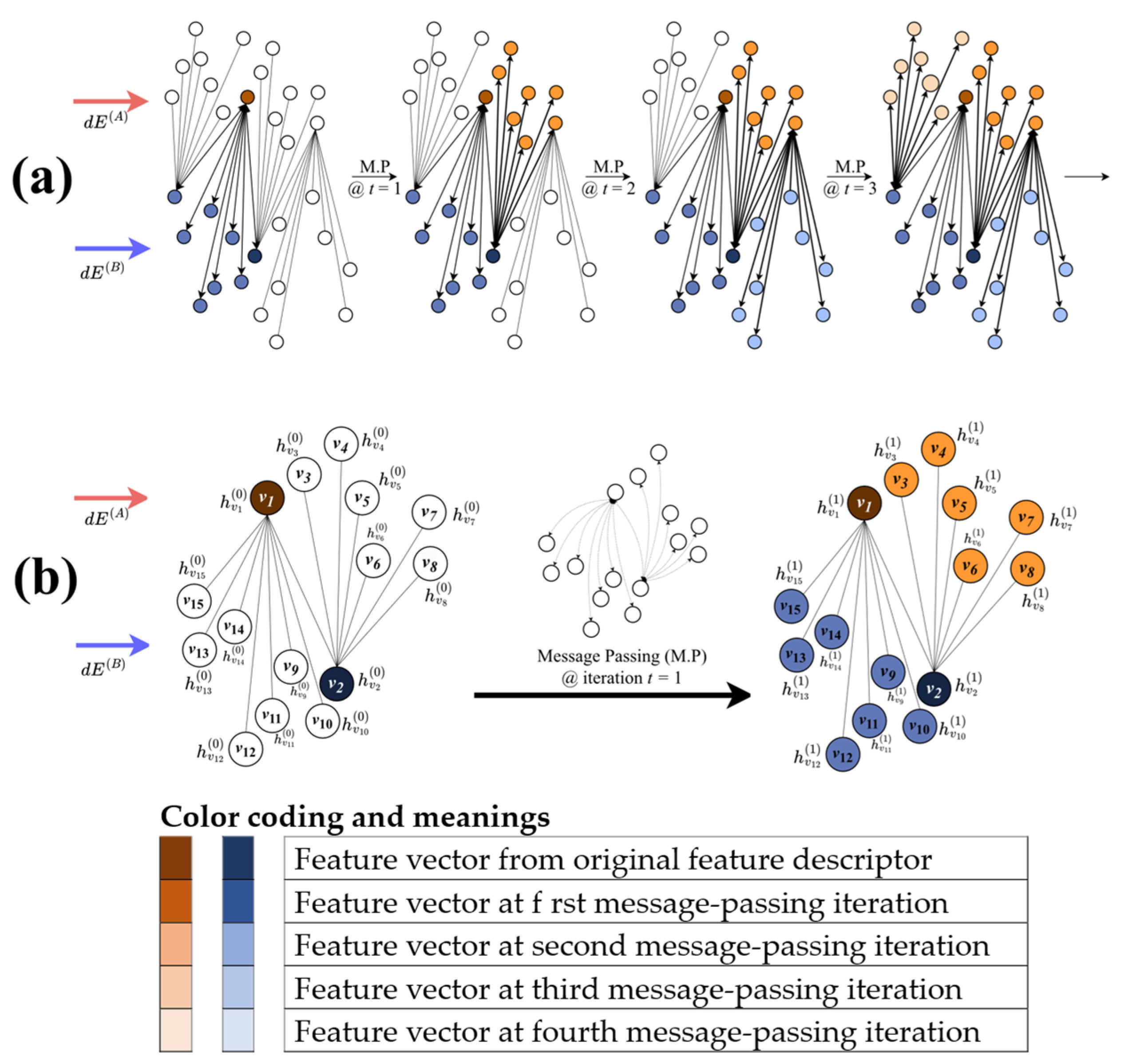
Message Passing in h-GNN

After applying SC+PCA to increase the graph network’s depth, and initiating node representations of graphs in the network, the next step is to develop efficient message-passing mechanisms that will update the initial node representations of graphs in the h-GNN. These mechanisms ensure that local and global information are propagated among nodes and graphs (i.e., within and across hierarchical levels of the h-GNN). It is important to note that SC+PCA inherently preserves both local and global information. Therefore, developing message-passing mechanisms that also ensure the propagation of both local and global information provides a dual benefit to our proposed h-GNN. As mentioned previously, the message-passing mechanism in h-GNN performed at an $l$-th level of hierarchy comes in four types.

1.

Within-level Message Propagation: This type adopts the general standard message-passing mechanism of SuperGlue [2]. To further enrich initial node representations, these representations are iteratively refined by updating and aggregating information received from neighboring nodes within the same graph ${\mathcal{G}}^{\left(l\right)}$. Basically, communication between nodes within a graph at a particular hierarchical level updates the initial node representations of the graph. Node representations are initiated with attention mechanisms. Following the general definition given by [32] of the standard message-passing mechanism, the $t$-th iteration of the within-level message passing to improve the node representation beyond the initial node representations can be expressed as

$$m_{v_j^{\left(l\right)}}^{\left(t\right)}={\mathrm{M}\mathrm{S}\mathrm{G}}^{\left(t\right)}\left\{\left(h_{v_j^{\left(l\right)}}^{\left(t-1\right)}\right)|\forall v_j^{\left(l\right)}\in \mathrm{N}\mathrm{B}\mathrm{R}\left(v_i^{\left(l\right)}\right) \mathrm{s}.\mathrm{t}.{\mathrm{A}}^{\left[1,\mathsf{\delta }\right]}\right\}$$

(7)

$$h_{v_i^{\left(l\right)}}^{\left(t\right)}={\mathrm{A}\mathrm{G}\mathrm{G}}^{\left(k\right)}\left(m_{v_j^{\left(l\right)}}^{\left(t\right)},h_{v_i^{\left(l\right)}}^{\left(t-1\right)}\right)$$

(8)

In Equation (7), $h_{v_j^{\left(l\right)}}^{\left(t-1\right)}$ is the previous representation of node $v_j^{\left(l\right)}$ at the $t-1$-th iteration of the message-passing process. This representation captures the information available at node $v_j^{\left(l\right)}$ prior to receiving messages from its neighboring nodes during the $t$-th iteration. Therefore, for the first message-passing iteration ($t=1$), the ‘previous’ node representation $h_{v_j^{\left(l\right)}}^{\left(t-1\right)}$ is actually the initial node representation, since no message-passing has occurred yet. This is denoted as $h_{v_j^{\left(l\right)}}^{\left(t-1\right)}=h_{v_i}^t$ if $t=1$.

The function ${\mathrm{M}\mathrm{S}\mathrm{G}}^{\left(t\right)}\left(·\right)$ represents the message aggregation mechanism, which aggregates information from neighboring nodes to compute the message. The $m_{v_j^{\left(l\right)}}^{\left(t\right)}$ is the message passed among the set of neighboring nodes $v_j\in \mathrm{N}\mathrm{B}\mathrm{R}\left(v_i\right)$), constrained to the $\mathsf{\delta }$-degree adjacency matrix ${\mathrm{A}}^{\left[1,\mathsf{\delta }\right]}\in {\left\{0,1\right\}}^{n\times n}$ ($n$ denotes the number of keypoint nodes), which describes the sharing of information between nodes that are $\mathsf{\delta }$-degrees of separation apart, skipping intermediate neighbor nodes when $\mathsf{\delta }>1$.

In Equation (8), the improved node representation $h_{v_i^{\left(l\right)}}^{\left(t\right)}$ at node $v_i^{\left(l\right)}$ and iteration $t$ is computed based on the received messages and the previous representation, i.e., $h_{v_i^{\left(l\right)}}^{\left(t\right)}$ is the improved node representation of the node $v_i^{\left(l\right)}$ after receiving information passed from its neighbor node $v_j^{\left(l\right)}$. The function ${\mathrm{A}\mathrm{G}\mathrm{G}}^{\left(t\right)}\left(·\right)$ denotes the aggregation mechanism, which combines the received messages and the previous representation to compute the updated node representation.

Equations (7) and (8) combine for the within-level message-passing process in the h-GNN, where information is exchanged between neighboring nodes (Equation (7)) and aggregated to update node representations within a graph of a particular hierarchy (Equation (8)). The δ-degree adjacency matrix controls the propagation of information, ensuring that information is exchanged only between nodes that are δ-degrees of separation apart.

To consider a practical application of Equations (7) and (8) in our context of image feature matching, $m_{v_j^{\left(l\right)}}^{\left(t\right)}$ represents the message passed from neighboring keypoints to the keypoint at iteration $t$. These messages encode information about the spatial positions and visual appearances of keypoints within a local neighborhood of the keypoint $v_j^{\left(l\right)}$. The function ${\mathrm{M}\mathrm{S}\mathrm{G}}^{\left(t\right)}\left(·\right)$ aggregates this information and incorporates them as, for instance, geometric (homography) transformations to align keypoints between the two images. The updated keypoint representation $h_{v_i^{\left(l\right)}}^{\left(t\right)}$, at iteration $t$, combines (aggregates) the received messages $m_{v_j^{\left(l\right)}}^{\left(t\right)}$ from neighboring keypoints and the previous representation $h_{v_i^{\left(l\right)}}^{\left(t-1\right)}$. The function ${\mathrm{A}\mathrm{G}\mathrm{G}}^{\left(t\right)}\left(·\right)$ performs this aggregation process, which in a practical sense could involve attention mechanisms to prioritize informative messages from neighboring keypoints.

2.

Bottom-up Message Propagation. After obtaining the node representations $h_{v_i}^{\left(k\right)}$ within all graphs ${\mathcal{G}}^{\left(l\right)}$, we perform the bottom-up type of message passing. In this type, directed messages propagate from a node in the graph ${\mathcal{G}}^{(l-1)}$ to the corresponding mega-node in the mega-graph ${\mathcal{G}}^{\left(l\right)}$. This enriches node information by aggregating from lower levels to higher levels in the hierarchy. Still following the general definition of GNN’s message passing in [32], the node representations are updated through bottom-up message propagation as follows:

$$m_{v_i^{\left(l\right)}}^{\left(t\right)}={\mathrm{M}\mathrm{S}\mathrm{G}}^{\left(t\right)}\left\{\left(h_{v_i^{\left(l-1\right)}}^{\left(t\right)}\right)|\forall v_i^{\left(l-1\right)}\in V_i^{\left(l-1\right)}\right\},$$

(9)

$$h_{v_i^{\left(l\right)}}^{\left(t\right)}={\mathrm{A}\mathrm{G}\mathrm{G}}^{\left(t\right)}\left(m_{v_i^{\left(l\right)}}^{\left(t\right)},h_{v_i^{\left(l\right)}}^{\left(t\right)}\right)$$

(10)

The rationale for presenting Equations (9) and (10) in this manner is similar to that of the previous equations, i.e., Equations (7) and (8). The breakdowns for these equations are therefore similar. For example, $v_i^{\left(l\right)}$ is a mega-node in ${\mathcal{G}}^{\left(l\right)}$, and $v_i^{\left(l-1\right)}\in V_i^{\left(l-1\right)}$ is its corresponding node in the graph ${\mathcal{G}}^{(l-1)}$ of the previous hierarchical level $l-1$. Also, $h_{v_i^{\left(l-1\right)}}^{\left(t\right)}$ represents the within-level node representation of $v_i$ at level $l-1$ and message-passing iteration $t$. In the hierarchical structure, $l-1$ denotes a lower level directly to $l$. Again, $h_{v_i^{\left(l\right)}}^{\left(t\right)}$ is the updated within-level node representation after bottom-up message propagation. The practical application of the ${\mathrm{M}\mathrm{S}\mathrm{G}}^{\left(t\right)}\left(·\right)$ and the ${\mathrm{A}\mathrm{G}\mathrm{G}}^{\left(t\right)}\left(·\right)$ functions in Equations (9) and (10) are also similar to the previous Equations (7) and (8).

We further adopt two top-down types of message-passing mechanisms among graphs of different hierarchical levels. We termed the two types Type-1 and Type-2.

3.

Type-1 Top-down Level Message Propagation: This is the direct reverse of the bottom-up type of message passing, where in order to update the node representations $h_{v_i^{\left(l\right)}}^{\left(t\right)}$, messages are directed from a mega-node in the mega-graph ${\mathcal{G}}^{\left(l\right)}$ to the corresponding node in the graph ${\mathcal{G}}^{(l-1)}$). This type of message passing updates node representations $h_{v_i^{\left(l-1\right)}}^{\left(t\right)}$ of graph ${\mathcal{G}}^{(l-1)}$) by aggregating discriminative features of nodes from higher levels to lower levels in the hierarchy, as follows:

$$h_{v_i^{\left(l-1\right)}}^{\left(t\right)}={\displaystyle \frac{1}{\left|v_i^{\left(l-1\right)}\right|+1}}\left(\sum _{v_i^{\left(l\right)}\in V_i^{\left(l\right)}}{h}_{v_i^{\left(l\right)}}^{\left(t\right)}+h_{v_i^{\left(l-1\right)}}^{\left(t\right)}\right)$$

(11)

From Equation (11), ${\displaystyle \frac{1}{\left|v_i^{\left(l-1\right)}\right|+1}}$ is a normalization factor, whereby $\left|v_i^{\left(l-1\right)}\right|+1$ represents the number of nodes in the set $V_i^{\left(l-1\right)}$, which consists of nodes at hierarchical level $l-1$ that are connected to node $v_i^{\left(l\right)}$. Adding one accounts for the original node itself and it ensures that the normalization includes both the sum of its neighbors’ contributions and its own current representation. This summation term aggregates the feature representations $h_{v_i^{\left(l\right)}}^{\left(t\right)}$ of mega-nodes $v_i^{\left(l\right)}$ at the higher level $l$ and the feature representations $h_{v_i^{\left(l-1\right)}}^{\left(t\right)}$ that represent the node $v_i^{\left(L-1\right)}$ at the lower level $l-1$.

To consider a practical application of Equation (11) in our context of image feature matching, the equation helps pass messages in a top-down manner, where it gathers information from higher-level nodes to be used for updating the lower-level node representations. The purpose is to refine and update the detailed node features at lower levels based on the more meaningful, aggregated information from higher levels.

4.

Type-2 Top-down Level Message Propagation: This type is where we update the node representations $h_{v_i}^{\left(t\right)}$ of original nodes $v_i$ of the base graphs $\mathcal{G}$ with the node representations $h_{v_i^{\left(L\right)}}^{\left(t\right)}$ of the global node $v_i^{\left(L\right)}\in V_i^{\left(L\right)}$ of the global graph ${\mathcal{G}}^{\left(L\right)}$. This updates node information by aggregating from the highest level in the hierarchy to the lowest level and could be expressed as

$$h_{{\mathit{v}}_{\mathit{i}}}^{\left(t\right)}={\displaystyle \frac{1}{\left|v_i\right|+1}}\left(\sum _{v_i^{\left(L\right)}\in V_i^{\left(L\right)}}{h}_{v_i^{\left(L\right)}}^{\left(t\right)}+h_{v_i}^{\left(t\right)}\right)$$

(12)

The breakdowns for Equations (11) and (12) are also similar. From Equation (12), ${\displaystyle \frac{1}{\left|v_i\right|+1}}$ is a normalization factor, whereby $\left|v_i\right|+1$ represents the number of original nodes in the set $V_i$, which consists of nodes at the base graph. Adding one accounts for the original node itself, and it ensures that the normalization includes both the sum of the neighbors of the original node contributions and its own current representation. This summation term aggregates the feature representations $h_{v_i^{\left(L\right)}}^{\left(t\right)}$ of global node $v_i^{\left(L\right)}$ at the highest hierarchical level $L$ and the feature representation $h_{v_i}^{\left(t\right)}$ that represents the original node $v_i$ at the lowest hierarchical level of the base graph.

To consider a practical application of Equation (12) in our context of image feature matching, the equation also helps pass messages in a top-down manner, where it gathers information from the highest-level nodes to be used for updating the lowest-level node representations. The purpose is to refine and update the detailed node features at the lowest level based on the more meaningful, aggregated information from the highest level. The four types of message-passing mechanisms are illustrated in Figure 6 below:

2.2.3. Matching Module

The inputs to the matching module are the enriched and distinctive keypoint descriptors associated with respective nodes. The matching module performs an iterative optimization on these enriched descriptors to obtain the matching results, which are represented as a partial assignment matrix. Thus, this module produces a partial assignment matrix. This is illustrated in the detailed overview of the h-GNN in Figure 2. Through the graph construction module (i.e., the GNN module) of the h-GNN, the enriched keypoint feature descriptors $\left(d_{\left(pos\right)}^{\left(*\right)},d_{\left(vis\right)}^{\left(*\right)}\right)$ for each image in the pair are transformed into distinct feature descriptors $f_i^{\left(A\right)}$ and $f_i^{\left(B\right)}$. These transformed descriptors are further enriched with local and global information, serving as robust representations for feature matching. Then, the matching layer performs an iterative optimization to obtain the matching results on these transformed descriptors $f_i^{\left(A\right)}$ and $f_i^{\left(B\right)}$ as a partial soft assignment matrix ${\left[\mathcal{P}\right]}_{M\times N}\in \left[0,1\right]$, where $M$ is number of local and global features in $f_i^{\left(A\right)}$ and $N$ is number of local and global features of $f_i^{\left(B\right)}$.

First, a pairwise matching score matrix ${\left[\mathcal{S}\right]}_{M\times N}$ is obtained by maximizing a score function between the feature descriptors, similar to solving any normal optimization problem through an iterative procedure. A higher matching score ${\mathit{s}}_{\mathit{i}\mathit{j}}\in \mathcal{S}$ from the function represents a higher match between two features. Thus, if we perform an iterative process to arrange all feature descriptors in the image $I^{\left(A\right)}$ vertically and all feature descriptors in the image $I^{\left(A\right)}$ horizontally, the score matrix, which contains scores of all possible correct matches, will be constructed. The score matrix $\mathcal{S}$ is augmented into an $\left(M+1\right)\times \left(N+1\right)$ dimension by a special case of a matrix with particular characteristics. The matrix is specially characterized such that it has non-empty row and column vectors, intersecting at their last elements. This is termed as a dustbin, and it is essentially a $1\times 1$ matrix appended to allow matrix $\mathcal{S}$ to suppress unmatched features between the descriptors. The score matrix and its appended $\left(\oplus \right)$ $r\times c$ dustbin matrix can be represented as

$${\left[\mathcal{S}\right]}_{\left(M+1\right)\times \left(N+1\right)}={\left[\mathcal{S}\right]}_{M\times N}\oplus \left(r_1,r_2,\dots ,r_m,r_{m+1}\right)\left(\begin{array}{c}{c}_1\\ c_2\\ ⋮\\ c_n\\ c_{n+1}\end{array}\right)│ r_{m+1}=c_{n+1}$$

(13)

Another optimization problem, the optimal transport problem, is also solved using the Sinkhorn algorithm. The algorithm is a commonly used efficient algorithm for solving optimal transport problems. The Sinkhorn algorithm translates all scores in the score matrix ${\left[\mathcal{S}\right]}_{M\times N}$ into percentages, which means the sum of any column or row should be one. The principle of the Sinkhorn algorithm is to divide each element of a row/column by the sum of that row/column so that the sum of that row/column becomes 1. The process of applying the Sinkhorn algorithm to all rows/columns in the score matrix is called row/column normalization. The optimal matching layer will iterate row and column normalization $T$ times until the sum of every row and column is 1, and the result is the final partial assignment matrix ${\left[\mathcal{P}\right]}_{\left(M+1\right)\times \left(N+1\right)}$. The dustbin matrix can be dropped and the dimension of $\mathcal{P}$ can be recovered to ${\left[\mathcal{P}\right]}_{M\times N}$.

2.2.4. Loss Functions

Two loss functions are used for the respective modules of the h-GNN. These loss functions are the reprojection loss ${\mathcal{L}}_{rp}$ and the dual non-contrastive clustering losses ${\mathcal{L}}_c^{\left(l\right)}$ Details regarding the reprojection loss ${\mathcal{L}}_{rp}$ and the clustering loss ${\mathcal{L}}_c^{\left(l\right)}$ are provided as follows:

Dual Non-contrastive Clustering Loss: This is a GNN module loss. Following [33], a dual non-contrastive clustering loss ${\mathcal{L}}_c^{\left(l\right)}$ was also implemented to semi-supervise clearer clustering partition and can be formulated as follows:

$${\mathcal{L}}_c^{\left(l\right)}={\displaystyle \frac{1}{C^{\left(l\right)}}}\left(\sum _{i,j=1}^{C^{\left(l\right)}}{\displaystyle \frac{{\mathrm{u}}_i·\mathcal{T}\left({\left\{{\mathrm{u}}_j^{\prime }\right\}}_{j\ne i}^{C^{\left(l\right)}}\right)}{‖{\mathrm{u}}_i‖‖\mathcal{T}\left({\left\{{\mathrm{u}}_j^{\prime }\right\}}_{j\ne i}^{C^{\left(l\right)}}\right)‖}}-\sum _{i=1}^{C^{\left(l\right)}}{\displaystyle \frac{{\mathrm{u}}_i·{\mathrm{u}}_i^{\prime }}{‖{\mathrm{u}}_i‖‖{\mathrm{u}}_i^{\prime }‖}}\right)$$

(14)

where $\mathcal{T}\left(·\right)$ denotes an operation that selects representative cluster centers from a set of clusters, and $C^l$ indicates the cluster $C$ at a particular hierarchical level $l$. The first term promotes differentiating dissimilar cluster center pairs $\left({\mathrm{u}}_i,{\mathrm{u}}_j\right)$ of different mega-graphs, and the second term encourages consistency within cluster center pairs $\left({\mathrm{u}}_i,{\mathrm{u}}_i^{\prime }\right)$ that could represent the same mega-graph at the next hierarchical level of clustering.

Reprojection Loss: This is a matching module loss that facilitates the semi-supervised optimization of keypoint match positions. This initially generates keypoint matches $\mathcal{M}$ between image pairs $\left(I^{\left(A\right)},I^{\left(B\right)}\right)$ using a feature descriptor and a matching algorithm. Subsequently, we estimate the $3\times 3$ homography matrices, ${\mathrm{H}}^{\left(AB\right)}$ (applicable to both indoor and outdoor tasks), between the image pair using the matched keypoints. For each task, the homography is applied to the keypoints in $I^{\left(A\right)}$, first projecting their locations onto the coordinate reference system of $I^{\left(A\right)}$ with

$$\left[{\left({\mathcal{M}}^{\left(AB\right)}\right)}^T,1\right]={\mathrm{H}}^{\left(AB\right)}{\left[{{\mathcal{M}}^{\left(A\right)}}^T,1\right]}^T$$

(15)

and second, reprojecting keypoint match ${\mathcal{M}}^{\left(AB\right)}$ by finding its closest detected keypoint match ${\mathcal{M}}^{\left(B\right)}$ within the threshold ${th}_{rp}$ of pixel distance. Then, the reprojection distance of ${\mathcal{M}}^{\left(AB\right)}$ and ${\mathcal{M}}^{\left(B\right)}$ is computed as

$${\mathrm{dist}}^{\left(AB\right)}={‖{\mathcal{M}}^{\left(AB\right)}-{\mathcal{M}}^{\left(B\right)}‖}_p$$

(16)

where $p$ represents the norm factor. To ensure reprojection loss, consider the reprojection distance in both directions, i.e., from image $I^{\left(A\right)}$ to image $I^{\left(B\right)}$ and from image $I^{\left(B\right)}$ to image $I^{\left(A\right)}$, symmetrically, where we obtain the following:

$${\mathcal{L}}_{rp}={\displaystyle \frac{1}{2}}\left({\mathrm{dist}}^{\left(AB\right)}+{\mathrm{dist}}^{\left(BA\right)}\right)$$

(17)

Minimizing the reprojection loss involves bringing the initially projected keypoint match and its associated keypoints closer together by adjusting their positions. With the acquisition of a pairwise matching score matrix $\mathcal{S}$, the adjustment of keypoint positions occurs in a unified optimization step, focusing on optimizing the scores within $\mathcal{S}$ that correspond to each keypoint.

3. Experiments and Discussions

This section is dedicated to explaining the strategies used to evaluate our proposed method. We compare the performance of our method to baseline methods on several datasets and metrics. A discussion subsection is also included to highlight the benefits and challenges of the proposed method.

3.1. Platform

Our proposed h-GNN model is implemented in a PyTorch framework. All experiments are performed on a Windows PC with a Ryzen 7 3700X 3.60 GHz CPU, 32 GB RAM, and an NVIDIA RTX 3080 GPU.

3.2. Implementation Setup

We utilized the Adam optimizer with an initial learning rate of 1e-4 and a batch size of 32. Our model employs multi-head self- and cross-attention with four heads across six hierarchical levels. Hierarchical levels are determined by $k$-means clustering with $k=5$ and $b=2$, iterated five times with incremental partitioning {$8, 16, 32, 64, 128\}$. This results in five hierarchical levels for the compressed-sized graphs and one hierarchical level for the base graph, making a total of six hierarchical levels of graphs. This is analogous to stacking nine layers, as in the case of other ‘Glue’-based GNN feature matchers. Base graphs and each hierarchical level comprise two self-edges and one cross-edge cluster-based GNN attention layer. We set $\mathsf{\delta }=2$, computing the first and second matrix powers of the adjacency matrix $\mathbf{A}$. This allows for flexibility in node connectivity, incorporating nodes at one $\left(\delta =1\right)$ and two $\left(\delta =2\right)$ degree(s) of separation apart during message passing. For the matching module, we run the Sinkhorn algorithm for $T=100$ iterations with a confidence threshold of $0.2$ for soft assignments, following conventions of ‘Glue’-based GNN feature matchers. Following the aforementioned setup, we evaluated the h-GNN for the following computer vision tasks: homography estimation, RANSAC variants for camera pose estimation, and qualitative visualization. With homography estimation for outdoor and indoor camera poses, the essential matrix loss parameter $\lambda =0.1$ for the first 20k iterations, then was fixed to 0.5. Training finished after $~$500k iterations. A comparison of model sizes (set in megabytes—MB) and average running times (set in milliseconds—ms) is also presented as an evaluation strategy.

3.3. Evaluations

3.3.1. Homography Estimation

RANSAC and weighted DLT homography estimators are used on image pairs sampled using random photometric distortions [1,34].

Setup: The ‘HPatches’ dataset [35] and the ‘Oxford and Paris’ [36] datasets are chosen to complement each other in evaluating our model’s capabilities. Whilst HPatches [35] offers a limited number of image pairs per scene, evaluating the model’s ability to handle repeated features, ‘Oxford and Paris’ [36] provides diverse features. In computing reprojection loss, where homography is applied to project keypoint match locations of $I^{\left(A\right)}$ onto $I^{\left(B\right)}$, the threshold ${th}_{rp}$ is set to 3, 5, and 10, indicating 3-, 5-, and 10-pixels distances between the projected keypoint matches ${\mathcal{M}}^{\left(AB\right)}$ and the actual keypoint matches ${\mathcal{M}}^{\left(B\right)}$ in the second image of a given pair (see Equation (15) for reference). Also, we evaluate homography estimation using the ${th}_{rp}$ and calculate precision (P), recall (R), and accuracy (A). The results are presented as AUC curves for reprojection thresholds less than 3, 5, and 10 pixels.

Baseline Models: Input images are resized to $640\times 480$ pixels. Sparse matchers are evaluated with 1024 local features from SuperPoint [1]. For the handcrafted sparse method, the PyTorch implementation of the nearest neighbor (NN) matching with (w/) a mutual check [37] was evaluated. For the learned sparse matchers, we include the NN w/PointCN [38], and w/the Order-Aware Network (OA-Net) [39] as outlier rejectors. Deep matchers are also evaluated, including SGMNet [40], SuperGlue [2], LightGlue [3], and LifelongGlue [4]. Official models of these feature matchers are trained on the MegaDepth [41] outdoor datasets used. Impartially, the transformer-based dense matcher, LoFTR [42], is also evaluated, selecting the top 1024 predicted matches. The h-GNN is also evaluated as a sparse matcher using 1024-dimensional feature vectors as inputs, derived from our feature descriptor described in Section 2.1.

Results: The h-GNN outperforms baseline methods, achieving high precision, recall, and accuracy (85.4, 87.3, and 86.2 for HPatches; 90.4, 83.1, and 88.0 for Oxford and Paris) in homography estimations with RANSAC. Compared to deep matchers, the h-GNN shows higher precision but ranks slightly below the dense matcher LoFTR [42]. Despite sparse keypoints, the h-GNN exhibits a higher accuracy than LoFTR [42] at coarser thresholds of 5 and 10 pixels for RANSAC (79.4 and 82.7 for HPatches; 80.8 and 85.2 for Oxford and Paris). When estimating homographies with DLT, the results of the h-GNN show much more accurate estimates than sparse and dense bassline matchers. Notably, the h-GNN competes with the dense matcher LoFTR [42] in homography estimations, even with a least-squares solver like DLT (39.7, 72.7, and 83.1 for HPatches; 38.5, 74.2, and 78.4 for Oxford and Paris). We show these results in

Table 1. Comparison of precision, recall, accuracy, and AUC at three threshold values for homography estimations with RANSAC and DLT on ‘HPatches’ and ‘Oxford and Paris’ datasets. Bold texts indicate the best results. The downwards arrow with tip rightwards’ (↳) indicate a sub-item that is related to the main item above it.

Features Detector and Descriptor		P|R|A (HPatches) (Oxford and Paris)	AUC-RANSAC @ (3|5|10) px (HPatches) (Oxford and Paris)	AUC-Weighted DLT @ (3|5|10) px (HPatches) (Oxford and Paris)
↳	Matchers
SuperPoint
↳	NN w/mutual checks	(31.7|37.4|41.1) (33.4|40.1|46.8)	(32.1|39.5|42.6) (33.4|43.3|48.6)	(0.0|1.7|1.8) (0.1|1.3|1.6)
↳	NN w/PointCN	(52.1|55.3|57.8) (59.9|57.7|61.9)	(33.1|60.1|73.1) (33.8|73.8|78.4)	(15.8|35.3|44.6) (17.2|38.1|47.6)
↳	NN w/OA-Net	(57.9|60.6|63.2) (67.8|71.4|61.5)	(34.2|62.9|74.8) (33.9|73.1|78.5)	(19.8|1.3|49.6) (22.5|1.3|53.6)
↳	SGMNet	(63.0|64.6|67.9) (72.5|73.3|63.2)	(36.2|63.2|76.8) (35.5|73.1|79.9)	(32.3|58.1|69.8) (33.2|71.2|74.3)
↳	SuperGlue	(66.2|74.4|70.3) (71.7|75.1|74.1)	(37.3|63.5|79.4) (36.5|73.2|80.7)	(34.5|60.7|74.6) (34.1|71.6|74.4)
↳	LightGlue	(67.3|83.0|83.7) (73.7|77.2|73.7)	(38.1|69.8|80.1) (36.8|74.1|81.3)	(38.3|76.7|79.1) (36.7|72.5|74.5)
↳	LifelongGlue	(81.2|85.3|85.8) (88.6|83.3|87.4)	(40.5|69.4|80.2) (38.9|76.6|82.7)	(38.8|78.2|80.1) (36.4|72.8|75.8)
Our Feature Detector and Descriptor
↳	h-GNN	(85.4|87.3|86.2) (90.4|83.1|88.0)	(39.9|79.4|82.7) (42.9|80.8|85.2)	(39.7|72.7|83.1) (38.5|74.2|78.4)
Dense
↳	LoFTR	(94.9|92.2|92.7) (89.8|91.1|90.8)	(41.9|78.5|81.3) (45.4|78.1|84.4)	(39.1|72.2|85.3) (37.9|73.6|77.8)

.

3.3.2. Tests on RANSAC Variants for Outdoor and Indoor Camera Pose Estimation

Indoor and outdoor scene complexities make it challenging for camera pose estimation tests. Outdoor scenes may have objects dominant in the scene but often exhibit very minimal discriminative overlaps. Indoor scenes may have many overlaps or constraints with features of a variety of cluttered indoor objects. We will show that our approach works quite well under these complexities of the two environment scenes by evaluating the performance of our method and comparing it with several state-of-the-art methods in camera pose estimation tasks varying RANSAC.

Setup: The outdoor and indoor scene datasets selected are MegaDepth [41] and SUN3D RGBD [43]. MegaDepth [41] addresses visual overlap challenges, and scenes are split into training (60%), validation (20%), and test (20%) sets without overlapping scenes. We used 239 sequences out of the 254 scenes in the SUN3D [43] dataset as known scenes and the remaining 15 as unknown scenes for testing. The known scenes were further split into 80% training and 20% validation. Five RANSAC variants—DegenSAC, MAGSAC, PROSAC, GC-RANSAC, and LO-RANSAC—were used as robust estimators of five essential matrices, each decomposed into rotation and translation matrices for camera pose recovery. See [44] for detailed explanations and implementations of each variant. Again, the threshold ${th}_{rp}$ was set as in the previous setup for homography estimation. We generated projected keypoint matches ${\mathcal{M}}^{\left(AB\right)}$ and keypoint matches ${\mathcal{M}}^{\left(B\right)}$ of the second image $I^{\left(B\right)}$. We evaluated outdoor and indoor camera pose estimations using ${th}_{rp}$, calculating angular differences between estimated rotation and translation matrices of ${\mathcal{M}}^{\left(AB\right)}$ and ${\mathcal{M}}^{\left(B\right)}$. The results are summarized in terms of maximum angular error in rotation and translation, reporting the mean average precision (mAP) at the error threshold $5°$.

Baselines: The inputs of the h-GNN are putative descriptors of image keypoints, which are detected by our proposed feature detector and descriptor, discussed in Section 2.1. We kept this evaluation simple and used only the SuperPoint [1] feature descriptor and detector for all baselines for fair comparison. In our test data for both scenes, the average number of keypoint correspondences generated by our feature detector and by SuperPoint [1] is about 2000. The inliers predicted by the h-GNN are fed to robust estimators, i.e., RANSAC and its five variants, to recover the camera pose. Following [45], we select LFGC-Net, NN matching w/OA-Net [39], Sparse GANet, SGMNet [40], SuperGlue [2], LightGlue [3], and LifelongGlue [4] for comparison.

Results: 

Table 2. The mAP@$5^{\circ }$ of our method and baselines with different variants of RANSAC on the outdoor (MegaDepth) and indoor (SUN3D) dataset scenes. Bold texts indicate the best.

Baselines	RANSAC Variants	Camera Pose (Datasets)
		Outdoor (MegaDepth)	Indoor (SUN3D)
LFGC-Net	RANSAC	35.86	17.78
	DegenSAC	33.43	19.81
	MAGSAC	38.48	18.75
	PROSAC	32.86	16.86
	GC-RANSAC	33.12	15.29
	LO-RANSAC	33.78	16.03
Sparse GANet	RANSAC	46.36	21.5
	DegenSAC	44.24	23.78
	MAGSAC	48.44	22.35
	PROSAC	42.05	19.36
	GC-RANSAC	42.19	17.86
	LO-RANSAC	44.64	19.55
NN w/OA-Net	RANSAC	35.85	18.67
	DegenSAC	34.68	19.32
	MAGSAC	37.22	18.98
	PROSAC	34.25	17.17
	GC-RANSAC	34.38	15.24
	LO-RANSAC	34.42	15.02
SGMNet	RANSAC	43.46	17.21
	DegenSAC	41.38	20.62
	MAGSAC	44.36	18.18
	PROSAC	37.24	15.93
	GC-RANSAC	36.58	14.56
	LO-RANSAC	38.74	17.14
SuperGlue	RANSAC	46.02	21.93
	DegenSAC	44.8	22.23
	MAGSAC	47.8	22.57
	PROSAC	42.5	20.88
	GC-RANSAC	41.2	19.31
	LO-RANSAC	45.6	20.91
LightGlue	RANSAC	44.44	21.43
	DegenSAC	43.12	22.98
	MAGSAC	46.67	23.02
	PROSAC	40.42	18.73
	GC-RANSAC	41.95	17.81
	LO-RANSAC	42.02	19.94
LifelongGlue	RANSAC	43.61	21.14
	DegenSAC	42.46	23.66
	MAGSAC	44.86	21.91
	PROSAC	37.76	18.62
	GC-RANSAC	39.13	17.91
	LO-RANSAC	42.43	19.69
h-GNN	RANSAC	46.94	21.46
	DegenSAC	47.35	22.79
	MAGSAC	49.38	21.74
	PROSAC	42.96	19.93
	GC-RANSAC	42.31	21.19
	LO-RANSAC	45.55	18.87

reports the $\mathrm{m}\mathrm{A}\mathrm{P}@5°$. MAGSAC estimator generally outperforms the popular RANSAC in outdoor camera pose estimations. The top three results are in relation to the performance of combining the MAGSAC estimator with the h-GNN, Sparse GANet, and SGMNet, in that order. Specifically, MAGSAC’s performance with the h-GNN feature matcher is 0.94 mAP (i.e., the actual mAP is 49.38) more than the mAP computed for the performance of using MAGSAC as an estimator of the Sparse GANet feature matcher. Combining MAGSAC and Sparse GANet for outdoor camera pose estimation yields 0.64 mAP (i.e., the actual mAP is 48.44) in performance more than the performance of combining MAGSAC with SGMNet, which gives an actual mAP of 47.8. A similar result in favor of the MAGSAC estimator is noted by [45], and may be attributed to the fact that RANSAC’s predefined inlier threshold is suboptimal for large-scale outdoor image matching data like MegaDepth [41], with no scene overlaps, varying lighting, and regular structural changes, whereas MAGSAC’s marginalization approach improves its performance in those constraints. Next to MANSAC, DegenSAC and RANSAC estimators also performed better when combined with the h-GNN, particularly on the MegaDepth [41] outdoor scenes, yielding 47.35 and 46.94 mAPs, respectively, compared to LO-RANSAC, PROSAC, and GC-RANSAC, which all show comparatively lower performances in that order. Table 2 indicates a generally low performance of the evaluated image matching methods for indoor scene pose estimation. This could be attributed to the difficulty in maintaining constant dominant features during the creation of indoor scenes, as various cluttered objects and complex lighting conditions capable of altering the objects’ textures may be present in those scenes. The best performance is observed with DegenSAC estimators combined with Sparse GANet and LifelongGlue, achieving mAPs of 23.78 and 23.66, respectively. This is followed by a LightGlue matcher using an MAGSAC estimator, which achieves an mAP of 23.02. The fourth on the list of best-performing combinations is LightGlue+DegenSAC, which achieves an mAP of 22.98. The fifth on the list is our proposed model, the h-GNN feature matcher, combined with the DegenSAC as its estimator, which achieved an mAP of 22.79.

3.3.3. Qualitative Analysis of the Open-Source Dataset

Setup: To evaluate our proposed model’s real-world effectiveness, we conducted keypoint matching on a series of sequential images from Strach’s dataset. Specifically, we selected its ‘Semper statue Dresden’ image sequence, comprising three sampled images. This sequence was chosen for its challenging nature, with a smaller number of images leading to numerous repeated features on the surfaces of sampled images. This scenario poses a significant challenge for image matching methods, allowing us to evaluate the performance of our proposed method under such conditions. We selected two out of the three sequential images and inputted them into our model for keypoint matching, visualizing the resultant matched keypoints on the image pair.

Baselines: The result of the proposed model was to compare that of nine baselines. Our h-GNN uses its own proposed feature detector to identify and describe keypoints in images. We visualized the output of the h-GNN with the nine existing models, which are the transformer-based matching model (LoFTR [42]), Sparse GANet, LFGC-Net, and SuperPoint [1], combined with different gluing mechanisms like SuperGlue [2], LightGlue [3], and LifelongGlue [4]. Additionally, there are nearest-neighbor (NN)-based models with different outlier rejectors, like mutual checks, PointCN, and OA-Net.

Results: Two methods were adopted to present the qualitative results of the performance of the h-GNN in handling repeated features on the surfaces of the image pair. We first provide some visualized results, then, second, we list statistical results from the matching.

Figure 7 visualizes some of the matched results in the image datasets. It is evident that using NN matching w/PointCN, OA-Net, and mutual checks as outlier rejectors yielded the fewest correct feature correspondences. This indicates that these methods had the lowest matching precision among the baselines. Although the use of SuperPoint as a feature descriptor for ‘Glue’-based models can remove some outliers, it also produced few matches compared to that of the h-GNN. However, using SuperPoint as a feature descriptor for ‘Glue’-based models generally achieved better results than LFGC-Net and nearest-neighbor-based approaches because of its use of the iterative graph updating method. To make the matching results easier to identify in Figure 7, matches that are common to all baselines are indicated by red lines. Green lines indicate matches that are unique to a particular matching method. We observed a moderate number of such green lines in the outputs of our proposed h-GNN, and even more in LoFTR [42].

Below, we list statistical results from the matching. The number of correct matches visualized for each method in Figure 7 is listed in

Table 3. Statistical results (raw matches and inlier matches) of the Semper sequence from Strach’s dataset.

Matcher	Semper Statue Dresden from Strach’s Dataset
	Keypoints	Matches
LoFTR	1760	1624
h-GNN	1721	1589
SparseGANet	927	896
SuperPoint+SuperGlue	732	477
SuperPoint+LightGlue	707	470
SuperPoint+LifelongGlue	738	458
LFGC-Net	631	389
NN w/PointCN	622	355
NN w/OA-Net	583	336
NN w/mutual checks	574	333

. The table lists ‘Keypoints’, which denotes the number of keypoints detected and described as features, and ‘Matches’, which denotes the number of estimated true matches between the image pairs. Also, as shown in Table 3, the h-GNN has the highest number of feature correspondences, next after the transformer-based deep image matcher LoFTR [42]. This interprets the effectiveness and competitive performance of the h-GNN comparable to deep image feature matchers and other Sparse image matching SOTAs.

3.3.4. Computation Time and Memory Complexities

Improving the processing time and GPU memory requirements while maintaining the lightweight nature of matching performance is one of the main motivations for developing the h-GNN model.

Setup: Figure 8a–c report the memory (test and train) and time (train) usage for different numbers of detected keypoint features (#Features) on an NVIDIA RTX 3080 GPU with 12 GB memory.

Baselines: The runtime and memory of our method are compared with SuperGlue [2] and with LightGlue [3], a lightweight variant of SuperGlue.

Results: In Figure 8a, our proposed method, h-GNN, consumes almost the same memory as LightGlue [3] during testing when the number of features is smaller than 2 k, where, after that, LightGlue [3] consumes more memory than our proposed method. During testing, our proposed method reduces the memory required by Superglue [2] by an average of 23.1% and that of LightGlue [3] by an average of 4.8%. Also, as shown in Figure 8b, for training, our proposed method reduces the memory required by Superglue [2] by an average of 38.1% and that required by LightGlue [3] by an average of 6.8%. The h-GNN can also achieve a better runtime performance. As shown in Figure 8c, for testing 10 k keypoints in intervals of 1 k, the h-GNN reduces the runtime by an average of 26.14%, compared to Superglue [2], and reduces the runtime by an average of 7.1% compared to LightGlue [3]. These results confirm that Superglue [2] constrains training on low-resource platforms more than LightGlue, and even more than our proposed approach, and, hence, our approach can be comparatively considered as a lightweight version of GNN-based image matching methods.

3.4. Ablation Study

We performed ablation studies to establish the performance of our proposed h-GNN on a real-world computer vision task, i.e., the Structure from Motion (SfM) pipeline. We also conducted two more ablation studies to investigate the contributions of different components in our h-GNN architecture, first to prove the validity of the SC+PCA clustering technique, and second to prove the validity of the message-passing (MP) mechanism of the h-GNN model.

3.4.1. h-GNN’s Performance in SfM Pipeline

Given the h-GNN’s impressive performance in camera pose estimation, particularly in challenging outdoor environments, we further investigate its applicability within the Structure from Motion (SfM) pipeline, also specifically tailored for outdoor scenes. In the SfM pipeline, feature matching is a useful step in camera pose estimation before sparse-to-dense point cloud generation from 2D images. We compare the feature matching results of the h-GNN against other feature matchers using the SFM pipelines in a 3D reconstruction.

Setup: This evaluation strategy involves utilizing two outdoor image scenes. In Figure 9, the top results are for the ‘Temple’ Multi-View Stereo (MVS) dataset. The dataset consists of 312 views, which were MVS captured on a hemisphere of a plaster model of the “Temple of the Dioskouroi”. Although this dataset may be described as an indoor scene dataset, as the views are captured on a hemisphere, it may also be considered as an outdoor scene, as the views originate from a plaster reproduction model of the “Temple of the Dioskouroi” outdoor scenes. Again, in Figure 9, the bottom results are for the ‘Intermediate-Family’ outdoor image sequence (a model from the ‘Tanks and Temples’ dataset). The complete process of the SfM pipeline is carried out using VisualSFM v0.5.26 software. Here, we conducted experiments using the default feature matching method within the VisualSFM pipeline, comparing it with customized configurations where alternative feature matching methods proposed in the literature were integrated with the VisualSFM pipeline. Subsequently, the matched features are inputted into VisualSFM to generate sparse 3D points. Since sparse 3D points are difficult to visualize, they are then fed into the CMVS/PMVS plugin to create dense 3D points. It is expected that a customized configuration that produces a greater number of sparse 3D points, consequently, will also produce visually appealing dense 3D points of the model from the image sequence, when so many sparse 3D points are fed into the CMVS/PMVS plugin.

Baselines: In Figure 9, the first column displays the reconstruction results obtained using the default matching process of VisualSFM. VisualSFM inherently employs SIFT to generate feature matches and utilizes RANSAC for estimating the fundamental matrix before the coarse filtering of outliers occurs. The second column is when SuperGlue [2] is used to generate feature matches that are loaded with corresponding image datasets into VisualSFM, but maintaining the use of RANSAC to filter outliers. The third column is when the h-GNN is used to generate feature matches, whereas all other settings remain similar to that above.

Results: Here, performance evaluation relies on the number of generated 3D points in a sparse reconstruction. This approach is justified, since a higher count of 3D points indicates a more acceptable image matching method for the 3D reconstruction process. Figure 9 presents the results. It is evident from the figure that the default VisualSFM tends to overlook many structures, as indicated by the missing points in the regions zoomed in with the red-colored rectangular boxes. These regions visualize some of the holes and distorted structures in the reconstruction. However, compared to VisualSFM+SuperGlue and the default VisualSFM, it can be observed that our h-GNN method accurately captures these intricate details, recovering their structures and highlighting the edges of a more complete 3D model. The quantitative results, specifically the counts of 3D points (# pts) and projections (# proj), further support this observation about our proposed method (i.e., VisualSFM+h-GNN). We focus on zooming in on the regions of the worst and best results for clarity.

3.4.2. Effects of SC+PCA Clustering Technique on h-GNN

We conducted ablation studies on camera pose estimation, again for the MegaDepth [41]. The number of keypoints varied from 1K to 2K, depending on the number of clusters we wanted to consider in this ablation study. There was the need to use a higher number of keypoints for experiments that considered models with a lower number of clusters, i.e., for 8-, 16-, and 32-layer models (see

Table 4. The effects of fixing or varying the number of cluster layers. We report pose estimation accuracy under different thresholds based on MegaDepth, using 1k and 2k keypoints where needed.

Methods	Pose Estimation
	$5^{\circ }$	${10}^{\circ }$	${20}^{\circ }$
Fixed Clusters
h-GNN 8-L @2k	25.45	36.63	54.73
h-GNN 16-L @2k	33.61	49.24	66.12
h-GNN 32-L @2k	38.82	56.81	73.68
Varied Cluster @1k	46.94	61.73	77.28

). All other experimental setups as described in Section 3.3.2 were maintained, except that we only selected RANSAC as the robust estimator for the h-GNN implementation. Also, with this experiment, the mAP at three error thresholds, $5°$, $10°$, and $20°$, were reported. The ablation study proves the validity of h-GNN’s SC+PCA clustering technique. More specifically, the study demonstrated the effects of fixing or varying the number of clusters produced by the SC+PCA clustering technique. The number of GNN layers (clusters) is fixed at 8, 16, and 32 layers, denoted as 8-L, 16-L, and 32-L models. Thereafter, another model is designed where the number of graphs constructed is varied. With this model, the SC+PCA clustering technique is allowed to produce and adopt its number of graph clusters.

Our ablation strategy gradually increased the fixed size of clusters in the h-GNN from 8 to 16 to 32, whilst the full number of clusters were used for the ‘varying’ strategy. In this experiment, we evaluated the effect of fixing the number of clusters to {8, 16, or 32} versus our choice to use the full number of clusters produced by the SC+PCA clustering technique, i.e., the ‘varying’ strategy. As observed in Table 4, the h-GNN, with a fixed number of clusters, suffers from a significant drop in performance, even when the number of keypoints is doubled. When the SC+PCA clustering technique of the h-GNN is allowed to adopt its number of layers, the best performance for the model analysis is observed.

3.4.3. Effects of Message-Passing (MP) Mechanism on h-GNN

We conducted an ablation study on camera pose estimation, again for MegaDepth [41], and using RANSAC as the default robust estimator of the h-GNN. All other experimental setups as described in Section 3.3.2 were still maintained. The ablation study proves the validity of the h-GNN’s message-passing (MP) mechanism, such that different configurations of the h-GNN, with its corresponding MP, were experimented on, and we again report the mAP at three error thresholds, $5°$, $10°$, and ${20}^{\circ }$, for each configuration.

The first configuration removed the within-level MP mechanism from the h-GNN model to analyze its contribution (see the case of ‘h-GNN w/only Within-level’ in

Table 5. The effects of varying h-GNN configurations, where each configuration uses only one type of message-passing mechanism. Pose estimation accuracy is reported under different thresholds based on MegaDepth.

Methods	Pose Estimation
	$5^{\circ }$	${10}^{\circ }$	${20}^{\circ }$
h-GNN w/only Within-level	42	56.93	71.87
h-GNN w/only bottom-up MP	42.65	57.35	73.03
h-GNN w/only Type-1 MP	42.63	57.36	73.03
h-GNN w/only Type-2 MP	43.33	58.11	74.55
Full h-GNN configuration	46.94	61.73	77.28

). This configuration produces an h-GNN model that maintains only the default MP, i.e., the within-level message propagation. This ‘h-GNN w/only Within-level’ configuration uses the standard message-passing mechanism of SuperGlue [2] and is general to most ‘Glue’-based feature matching methods. We also designed three other configurations of the h-GNN, each configuration using only one of the remaining three types of message-passing mechanism, either bottom-up, Type-1 top-down level, or top-down level message propagation mechanisms (see the cases of ‘h-GNN w/only Bottom-up MP’, ‘h-GNN w/only Type-1 MP’, and ‘h-GNN w/only Type-2 MP’ in Table 5). Moreover, we compared our proposed h-GNN at its full configuration, where all four types of message propagation mechanisms are used (see the case of ‘Full h-GNN configuration’ in Table 5). These configurations help us to investigate whether our proposed h-GNN without any modifications gives rise to the overall best performance, to analyze the importance of MP on the h-GNN.

From Table 5, we find that the full h-GNN configuration significantly outperforms the other configurations of h-GNN, which used only one type of message-passing mechanism, demonstrating the effectiveness of using all four types of MP on h-GNN. Specifically, the full h-GNN yields roughly 3 mAP at $5^{\circ }$, ${10}^{\circ }$, and ${20}^{\circ }$ error thresholds, more than the h-GNN configured to have only the Type-2 MP mechanism. Even though the h-GNN configuration with Type-2 MP outperforms the other configurations, except for the full h-GNN, the improvement of the h-GNN configuration with the Type-2 MP over the other configurations is relatively small. We also observe no significant difference in mAP values between configurations with bottom-up and Type-1 message propagations. We can attribute this observation to the fact that the Type-1 MP is a direct reverse of the bottom-up type of MP. Again, the results are shown in Table 4 and Table 5, where the mAP@$5^{\circ }$ error thresholds are reported for the ablation experiments. These results are similar to the results in Table 2, where the h-GNN was combined with the RANSAC robust estimator for homography estimation. They all yield 46.94 for mAP@$5^{\circ }$.

3.5. Discussions

The evaluation of the h-GNN against baseline methods in homography estimation on image datasets with repeated or diverse features considered three main aspects: the careful selection of baseline methods categorized as handcrafted or deep and sparse or dense matching methods; the variation of reprojection distances between keypoints; and the careful selection of homography estimators across two main categories: least-squares solvers, such as DLT, and iterative robust model fitting methods, such as RANSAC. For robust estimators, the results showed that the h-GNN outperforms baseline methods in both handcrafted and deep sparse methods and competes closely with deep dense matchers at coarser reprojection distances. For least-squares solvers, the h-GNN demonstrated significantly more accurate estimates than sparse baseline matchers, while remaining competitive with dense matchers in homography estimation.

The evaluation of the h-GNN against baseline methods on image datasets with varying complexities in indoor and outdoor scene environments offers valuable insights into the benefits and deficiencies of our proposed method. One significant benefit is the h-GNN’s robust performance in outdoor scene complexities, showcasing its ability to effectively handle images with diverse features and repeated patterns. Moreover, the h-GNN demonstrates versatility by seamlessly integrating with various RANSAC variants for camera pose estimation. Particularly in outdoor scene pose estimation, the h-GNN combined with MAGSAC surpasses other methods, indicating its superior performance in challenging outdoor environments. However, a major deficiency emerges, as the h-GNN exhibits a relatively lower performance in indoor scene pose estimation. This drawback may be attributed to the inherent difficulties in maintaining consistent features within cluttered indoor environments, posing challenges in feature matching and camera pose estimation. Despite its success in outdoor scenes, this limitation underscores the need for further refinement to enhance the h-GNN’s performance in indoor settings.

The qualitative analysis also highlights the h-GNN’s benefits in real-world scenarios, particularly in challenging environments. It reveals that when compared to transformer-based deep image matchers, the h-GNN outperforms other sparse matchers by achieving the highest number of feature correspondences. This highlights the h-GNN’s capability to handle repeated features on image surfaces effectively, consistently producing a high number of correct feature correspondences in challenging scenarios. However, the effectiveness of the h-GNN is deficient, as it is heavily reliant on its proposed feature detector for identifying and describing keypoints in images, and its performance may vary with different feature detectors, particularly those whose design architectures are different from SuperPoint and SuperGlue.

Generally, the findings highlight the effectiveness of the h-GNN as a sparse matcher, particularly when paired with robust estimators like MAGSAC and RANSAC, demonstrating superior performance in homography estimation tasks, especially in outdoor scenes. We have illustrated that the proposed matching method can achieve significant improvement in running time and memory usage, whilst maintaining a high matching accuracy in the above task. While our evaluation did not directly assess the application of our method on resource-limited devices, the observed improvements in time and memory suggest that such an evaluation would be feasible. These findings affirm that the h-GNN can be regarded as a lightweight GNN-based image matcher, offering promising prospects for practical implementation in various low-resource platforms. Specifically, the findings show that our proposed h-GNN is a lightweight GNN-based image matcher that achieves significant improvements in memory and time complexities in feature matching (by an average of 38.1% and 26.14% reduction in memory and runtime compared to SuperGlue [2] and 6.8% and 7.1% compared to LightGlue [3], a lightweight variant of SuperGlue [2]).

The experiments in the ablation study are three-fold; the first explores the performance of our proposed h-GNN on a Structure from Motion (SfM) pipeline, the second investigates the contribution of the SC+PCA clustering technique on the h-GNN, and the third investigates the contribution of message-passing mechanisms on the h-GNN.

The ablation study conducted on the h-GNN’s performance in 3D reconstruction using Structure from Motion (SfM) revealed its benefits over baseline methods, as it excelled in accurately capturing intricate points of the surfaces of 3D structures, free from holes and distortions, thereby highlighting the edges of 3D objects and producing more complete 3D models. This was evident in its ability to generate a higher number of 3D points compared to baseline methods. The increased count of 3D points signifies the h-GNN’s capability to generate denser and more accurate point clouds, indicating its effectiveness in image matching for Structure from Motion (SfM) tasks. Again, our ablation study conducted on the effects of the SC+PCA clustering technique on h-GNN revealed that allowing the technique to run its full number of iterations to produce and use its number of layers leads to the best performance for the h-GNN. Finally, the ablation study conducted on the effects of message-passing mechanisms on the h-GNN revealed that all four mechanisms combine to significantly improve the effectiveness of the h-GNN compared to when one type of message-passing mechanism is used for the h-GNN

4. Conclusions

In this paper, we propose the h-GNN, a lightweight GNN-based model for image feature matching. The h-GNN enhances message passing to capture both local and global information by leveraging hierarchical clustering. This hierarchical approach in itself preserves both local and global information on graphs. By adopting this method, the h-GNN efficiently passes messages between nodes with a compact attention pattern in graph networks. This contrasts with the prevalent practice of stacking multiple layers of complete graphs in GNNs for feature matching. Experimental results across various tasks and datasets demonstrate that the h-GNN improves feature matching accuracy and downstream task performance compared to state-of-the-art methods, all while requiring modest computational resources and memory. Thus, it can be concluded that the number of matches estimated by the h-GNN model is greater as compared to the majority of the sparse image matching models and even competes with the transformer-based dense image matching models. The h-GNN performs well in various challenging and complex scenarios, as it benefits from its message-passing capabilities that consider local and global information. Also, the h-GNN performs well, as it additionally benefits from the use of the clustering technique that preserves local and global information in graphs while increasing the network depth of the h-GNN. Our future research will aim to improve the adopted message-passing mechanisms, which are currently limited to only aggregating node feature representations. We will research into developing some recent types of simplicial message-passing mechanisms [46] that consider aggregating not only node feature representations but also edge feature representations in the message-passing process.

References

1. DeTone, D.; Malisiewicz, T.; Rabinovich, A. SuperPoint: Self-Supervised Interest Point Detection and Description. In Proceedings of the 2018 IEEE/CVF Conference on Computer Vision and Pattern Recognition Workshops, Salt Lake City, UT, USA, 18–23 June 2018; pp. 224–236. [Google Scholar] [CrossRef]
2. Sarlin, P.-E.; DeTone, D.; Malisiewicz, T.; Rabinovich, A. SuperGlue: Learning Feature Matching with Graph Neural Networks. In Proceedings of the 2020 IEEE/CVF Conference on Computer Vision and Pattern Recognition, Seattle, WA, USA, 13–19 June 2020; pp. 4938–4947. [Google Scholar] [CrossRef]
3. Lindenberger, P.; Sarlin, P.-E.; Pollefeys, M. LightGlue: Local Feature Matching at Light Speed. In Proceedings of the 2023 IEEE/CVF International Conference on Computer Vision, Paris, France, 1–6 October 2023; pp. 17627–17638. [Google Scholar] [CrossRef]
4. Zaman, A.; Yangyu, F.; Irfan, M.; Ayub, M.S.; Guoyun, L.; Shiya, L. LifelongGlue: Keypoint matching for 3D reconstruction with continual neural networks. Expert Syst. Appl. 2022, 195, 116613. [Google Scholar] [CrossRef]
5. Bellavia, F. Image Matching by Bare Homography. IEEE Trans. Image Process. 2024, 33, 696–708. [Google Scholar] [CrossRef] [PubMed]
6. Xu, M.; Wang, Y.; Xu, B.; Zhang, J.; Ren, J.; Huang, Z.; Poslad, S.; Xu, P. A critical analysis of image-based camera pose estimation techniques. Neurocomputing 2024, 570, 127125. [Google Scholar] [CrossRef]
7. Cao, M.; Jia, W.; Lv, Z.; Zheng, L.; Liu, X. SuperPixel-Based Feature Tracking for Structure from Motion. Appl. Sci. 2019, 9, 2961. [Google Scholar] [CrossRef]
8. Liu, Y.; Huang, K.; Li, J.; Li, X.; Zeng, Z.; Chang, L.; Zhou, J. AdaSG: A Lightweight Feature Point Matching Method Using Adaptive Descriptor with GNN for VSLAM. Sensors 2022, 22, 5992. [Google Scholar] [CrossRef] [PubMed]
9. Salimpour, S.; Queralta, J.P.; Westerlund, T. Self-calibrating anomaly and change detection for autonomous inspection robots. In Proceedings of the 6th IEEE International Conference on Robotic Computing, Naples, Italy, 5–7 December 2022; pp. 207–214. [Google Scholar] [CrossRef]
10. Le, V.P.; De Tran, C. Key-point matching with post-filter using sift and brief in logo spotting. In Proceedings of the 2015 IEEE International Conference on Computing & Communication Technologies-Research, Innovation, and Vision for Future, Can Tho, Vietnam, 25–28 January 2015; pp. 89–93. [Google Scholar] [CrossRef]
11. Xu, Y.; Li, Y.J.; Weng, X.; Kitani, K. Wide-baseline multi-camera calibration using person re-identification. In Proceedings of the IEEE/CVF Conference on Computer Vision and Pattern Recognition, Nashville, TN, USA, 20–25 June 2021; pp. 13134–13143. [Google Scholar] [CrossRef]
12. Zhou, Y.; Guo, Y.; Lin, K.P.; Yang, F.; Li, L. USuperGlue: An unsupervised UAV image matching network based on local self-attention. Soft Comput. 2023, 1–21. [Google Scholar] [CrossRef]
13. Ma, J.; Jiang, X.; Fan, A.; Jiang, J.; Yan, J. Image matching from handcrafted to deep features: A survey. Int. J. Comput. Vis. 2021, 129, 23–79. [Google Scholar] [CrossRef]
14. Khemani, B.; Patil, S.; Kotecha, K.; Tanwar, S. A review of graph neural networks: Concepts, architectures, techniques, challenges, datasets, applications, and future directions. J. Big Data 2024, 11, 18. [Google Scholar] [CrossRef]
15. Xu, J.; Chen, J.; You, S.; Xiao, Z.; Yang, Y.; Lu, J. Robustness of deep learning models on graphs: A survey. AI Open 2021, 2, 69–78. [Google Scholar] [CrossRef]
16. Wu, Z.; Pan, S.; Chen, F.; Long, G.; Zhang, C.; Philip, S.Y. A comprehensive survey on graph neural networks. IEEE Trans. Neural Netw. Learn. Syst. 2020, 32, 4–24. [Google Scholar] [CrossRef] [PubMed]
17. Gilmer, J.; Schoenholz, S.S.; Riley, P.F.; Vinyals, O.; Dahl, G.E. Message Passing Neural Networks. In Machine Learning Meets Quantum Physics; Schütt, K., Chmiela, S., von Lilienfeld, O., Tkatchenko, A., Tsuda, K., Müller, K.R., Eds.; Lecture Notes in Physics; Springer: Berlin/Heidelberg, Germany, 2020; Volume 968, pp. 199–214. [Google Scholar] [CrossRef]
18. Ahmed, A.; Shervashidze, N.; Narayanamurthy, S.M.; Josifovski, V.; Smola, A.J. Distributed large-scale natural graph factorization. In Proceedings of the 22nd International World Wide Web Conference, Janeiro, Brazil, 13–17 May 2013; pp. 37–48. [Google Scholar] [CrossRef]
19. Alon, U.; Yahav, E. On the bottleneck of graph neural networks and its practical implications. In Proceedings of the 9th International Conference on Learning Representations, Vienna, Austria, 3–7 May 2021; pp. 1–16. Available online: https://openreview.net/pdf?id=i80OPhOCVH2 (accessed on 10 April 2024).
20. Zhong, Z.; Li, C.T.; Pang, J. Hierarchical message-passing graph neural networks. Data Min. Knowl. Discov. 2023, 37, 381–408. [Google Scholar] [CrossRef]
21. Oono, K.; Suzuki, T. Graph neural networks exponentially lose expressive power for node classification. In Proceedings of the 8th International Conference on Learning Representations, Addis Ababa, Ethiopia, 26–30 April 2020; pp. 1–37. Available online: https://openreview.net/forum?id=S1ldO2EFPr (accessed on 10 April 2024).
22. Itoh, T.D.; Kubo, T.; Ikeda, K. Multi-level attention pooling for graph neural networks: Unifying graph representations with multiple localities. Neural Netw. 2022, 145, 356–373. [Google Scholar] [CrossRef] [PubMed]
23. Xu, K.; Hu, W.; Leskovec, J.; Jegelka, S. How powerful are graph neural networks? In Proceedings of the 7th International Conference on Learning Representations, New Orleans, LA, USA, 6–9 May 2019; pp. 1–17. Available online: https://openreview.net/pdf?id=ryGs6iA5Km (accessed on 10 April 2024).
24. Xu, K.; Li, C.; Tian, Y.; Sonobe, T.; Kawarabayashi, K.I.; Jegelka, S. Representation learning on graphs with jumping knowledge networks. In Proceedings of the 35th International Conference on Machine Learning, Stockholm, Sweden, 10–15 June 2018; pp. 5453–5462. Available online: https://proceedings.mlr.press/v80/xu18c.html (accessed on 10 April 2024).
25. Li, Q.; Han, Z.; Wu, X. Deeper insights into graph convolutional networks for semi-supervised learning. In Proceedings of the 2018 AAAI Conference on Artificial Intelligence, New Orleans, LA, USA, 2–7 February 2018; Volume 32, pp. 3538–3545. [Google Scholar] [CrossRef]
26. Zhou, S.; Liu, X.; Zhu, C.; Liu, Q.; Yin, J. Spectral clustering-based local and global structure preservation for feature selection. In Proceedings of the 2014 International Joint Conference on Neural Networks, Beijing, China, 6–11 July 2014; pp. 550–557. [Google Scholar] [CrossRef]
27. Wang, F.; Zhang, C.; Li, T. Clustering with local and global regularization. IEEE Trans. Knowl. Data Eng. 2009, 21, 1665–1678. [Google Scholar] [CrossRef]
28. Elisa, S.S. Graph clustering. Comput. Sci. Rev. 2007, 1, 27–64. [Google Scholar] [CrossRef]
29. Shun, J.; Blelloch, G.E. Ligra: A lightweight graph processing framework for shared memory. In Proceedings of the 18th ACM SIGPLAN Symposium on Principles and Practice of Parallel Programming, Shenzhen, China, 23–27 February 2013; pp. 135–146. [Google Scholar] [CrossRef]
30. Li, G.; Rao, W.; Jin, Z. Efficient compression on real world directed graphs. In Proceedings of the Web and Big Data 1st International Joint Conference, APWeb-WAIM, Beijing, China, 7–9 July 2017; pp. 116–131. [Google Scholar] [CrossRef]
31. Ma, E.J. Computational Representations of Message Passing—Essays on Data Science. 2021. Available online: https://ericmjl.github.io/essays-on-data-science/machine-learning/message-passing (accessed on 2 January 2024).
32. Fan, X.; Gong, M.; Wu, Y.; Qin, A.K.; Xie, Y. Propagation enhanced neural message passing for graph representation learning. IEEE Trans. Knowl. Data Eng. 2021, 35, 1952–1964. [Google Scholar] [CrossRef]
33. Tu, W.; Guan, R.; Zhou, S.; Ma, C.; Peng, X.; Cai, Z.; Liu, Z.; Cheng, J.; Liu, X. Attribute-Missing Graph Clustering Network. In Proceedings of the AAAI Conference on Artificial Intelligence, Vancouver, BC, Canada, 20–27 February 2024; Volume 38, pp. 15392–15401. [Google Scholar] [CrossRef]
34. Revaud, J.; De Souza, C.; Humenberger, M.; Weinzaepfel, P. R2D2: Repeatable and reliable detector and descriptor. arXiv 2019, arXiv:1906.06195. [Google Scholar]
35. Balntas, V.; Lenc, K.; Vedaldi, A.; Mikolajczyk, K. KHPatches: A Benchmark and Evaluation of Handcrafted and Learned Local Descriptors. In Proceedings of the IEEE/CVF Conference on Computer Vision and Pattern Recognition, Honolulu, HI, USA, 21–26 July 2017; pp. 3852–3861. [Google Scholar] [CrossRef]
36. Radenović, F.; Iscen, A.; Tolias, G.; Avrithis, Y.; Chum, O. Revisiting Oxford and Paris: Large-scale image retrieval benchmarking. In Proceedings of the IEEE/CVF Conference on Computer Vision and Pattern Recognition, Salt Lake City, UT, USA, 18–23 June 2018; pp. 5706–5715. [Google Scholar] [CrossRef]
37. Lowe, D.G. Distinctive image features from scale-invariant keypoints. Int. J. Comput. Vis. 2004, 60, 91–110. [Google Scholar] [CrossRef]
38. Yi, K.M.; Trulls, E.; Ono, Y.; Lepetit, V.; Salzmann, M.; Fua, P. Learning to find good correspondences. In Proceedings of the IEEE/CVF Conference on Computer Vision and Pattern Recognition, Salt Lake City, UT, USA, 18–23 June 2018; pp. 2666–2674. [Google Scholar] [CrossRef]
39. Zhang, J.; Sun, D.; Luo, Z.; Yao, A.; Zhou, L.; Shen, T.; Chen, Y.; Liao, H.; Quan, L. Learning two-view correspondences and geometry using order-aware network. In Proceedings of the IEEE/CVF International Conference on Computer Vision, Seoul, Republic of Korea, 27 October–2 November 2019; pp. 5845–5854. [Google Scholar] [CrossRef]
40. Chen, H.; Luo, Z.; Zhang, J.; Zhou, L.; Bai, X.; Hu, Z.; Tai, C.-L.; Quan, L. Learning to Match Features with Seeded Graph Matching Network. In Proceedings of the IEEE/CVF International Conference on Computer Vision, Montreal, QC, Canada, 11–17 October 2021; pp. 6301–6310. [Google Scholar] [CrossRef]
41. Li, Z.; Snavely, N. MegaDepth: Learning single-view depth prediction from internet photos. In Proceedings of the IEEE/CVF Conference on Computer Vision and Pattern Recognition, Salt Lake City, UT, USA, 18–23 June 2018; pp. 2041–2050. [Google Scholar]
42. Sun, J.; Shen, Z.; Wang, Y.; Bao, H.; Zhou, X. LoFTR: Detector-Free Local Feature Matching with Transformers. In Proceedings of the IEEE/CVF International Conference on Computer Vision, Montreal, QC, Canada, 11–17 October 2021; pp. 8922–8931. [Google Scholar] [CrossRef]
43. Xiao, J.; Owens, A.; Torralba, A. SUN3D: A Database of Big Spaces Reconstructed Using SfM and Object Labels. In Proceedings of the IEEE/CVF International Conference on Computer Vision, Sydney, Australia, 1–8 December 2013; pp. 1625–1632. [Google Scholar] [CrossRef]
44. Wang, W.; Sun, Y.; Liu, Z.; Qin, Z.; Wang, C.; Qin, J. Image matching via the local neighborhood for low inlier ratio. J. Electron. Imaging 2022, 31, 023039. [Google Scholar] [CrossRef]
45. Jiang, X.; Wang, Y.; Fan, A.; Ma, J. Learning for mismatch removal via graph attention networks. ISPRS J. Photogramm. Remote Sens. 2022, 190, 181–195. [Google Scholar] [CrossRef]
46. Truong, Q.; Chin, P. Weisfeiler and Lehman Go Paths: Learning Topological Features via Path Complexes. In Proceedings of the AAAI Conference on Artificial Intelligence, Vancouver, BC, Canada, 20–27 February 2024; Volume 38, pp. 15382–15391. [Google Scholar] [CrossRef]
Figure 1. General overview of steps, modules, and sub-steps of the proposed h-GNN. The h-GNN process initiates with keypoint detection from distinctive features in input images, followed by computing descriptors for each keypoint. Subsequently, feature matching identifies correspondences between keypoints across different images. The model enhances robust feature matching through two primary modules: the GNN module and the matching module. The GNN module operates on a graph representation of keypoints, initially constructing an input base graph where nodes represent keypoints. Employing clustering techniques increases the GNN’s depth, facilitating message-passing among neighboring nodes to update keypoint node representations with local and global contextual information. The output from the GNN module is input to the matching module. Under the matching module, a pairwise matching score matrix is computed between matches of updated keypoint nodes from different images. A dustbin matrix handles outlier keypoints lacking reliable matches. The Sinkhorn algorithm refines initial matching scores by iteratively adjusting assignment probabilities, resulting in a more accurate final partial assignment matrix.
Information 15 00602 g001
Figure 2. Technical details of the architecture and workflow of the proposed h-GNN. The workflow begins with the image inputs. Then, each of the image pair inputs is labeled as I ( A ) , and I ( B ) is processed by a keypoint detector, represented by different colored (red and blue) blocks. Keypoint descriptors D A and D ( B ) are also extracted from each image. After the image inputs’ section, the workflow can be divided into three main components. The first is the feature detection and description stage, where features are detected from both images. These features are encoded through two encoders, d E n c and k E n c , to produce keypoint descriptors. The second is the graph module, which consists of a base graph G representation for the keypoint descriptors. Self- and cross-attention layers enhance feature representations within each graph. The type of attention layers is differentiated by the curved arrows, which show the nature of interaction between the two types of graphs. The third is the matching module, where a score matrix representation is derived from matching keypoints. The Sinkhorn algorithm produces a partial assignment matrix P i j , indicating matches between keypoints in both images.
Information 15 00602 g002
Figure 3. Illustration of iterative process of increasing network depth in h-GNN, through the application of the SC+PCA clustering method. The starting point is a base graph G of original nodes labeled as v i V . At the first iteration of the SC+PCA technique, these original nodes are clustered into their respective “mega-node”. These mega-nodes form the mega-graph G 1 at hierarchical level l = 1 . This process is iterative. Mega-nodes from G 1 are further grouped into more complex structures, creating another layer of hierarchy. For instance, the second and third iterations result in the formation of new mega-graphs G 2 and G 3 at hierarchical levels l = 2 and l = 3 , respectively. The clustering progression continues iteratively until it reaches the last hierarchical level L , where global node v i L V creates the final global graph G L . At each hierarchical level, our proposed SC+PCA clustering method is applied to group nodes effectively.
Information 15 00602 g003
Figure 4. (a) Visualizing the self-edge attention type of the message-passing process for capturing local information in an image pair after two message-passing mechanism (M.P) iterations, i.e., before iteration t . (b) The scope of the information propagation is expanded along the M.P process. The node v 1 has its original node feature vectors, h v i t ,   i = 1 , 2 , 5 , at the base graph (left), i.e., @ before message-passing iteration t . Beyond the base graph, the M.P propagates node information between each pair of neighbor nodes, starting from the center node v 3 . As a result, each node representation is updated by aggregating its own information and neighbor information after the message passing (right), i.e., @ t = 1 . The color coding and meanings are presented below, after cross-edge visualization.
Information 15 00602 g004
Figure 5. (a) Visualizing the cross-edge type of the message-passing process for capturing local information in an image pair after two message-passing mechanism (M.P.) iterations, i.e., @ iteration t = 3 . (b) The scope of the information propagation is expanded along the M.P process. The node v 1 has its original node information, h v i t = 1 , 2 , 3 , , 10 , , 15 , at the base graph (left), i.e., before message-passing iteration t. Beyond the base graph, the M.P procedure propagates node information between each pair of connected nodes, starting from the center nodes v 1 of the first image and v 2 of the second image. As a result, each node has its own information and neighbor information after the message passing (right), i.e., @ t = 1 . The color coding and meanings are presented just above this description.
Information 15 00602 g005
Figure 6. (a) An illustration of the four types of message-passing mechanisms. (b) An alternative illustration of the message-passing mechanisms shown in (a). Message passing through nodes’ connections and across different hierarchical levels is illustrated with various dashed lines with directed arrows.
Information 15 00602 g006
Figure 7. Feature correspondences of the ‘Semper statue Dresden’ image sequence set from Strach’s dataset. Our proposed model, h-GNN, which combined our SuperPoint feature detector, is compared with nine other image matching models. The results show that the h-GNN has more robustness when it comes to repeated features than that of the other baselines.
Information 15 00602 g007
Figure 8. Efficiency comparison. We show the memory (testing and training) and time (training) usage with an increasing number of input features up to 10k.
Information 15 00602 g008
Figure 9. The dense reconstruction results of the various methods on two scenes. The top is the results from the image scene of the Temple MVS dataset, whilst the bottom is the results from the image scene of the ‘Family’ image sequence from the ‘Tanks and Temples’ dataset. For each image scene and method, the pair (# pts, # proj) represents the count of preserved 3D points and their corresponding projections utilized for dense reconstruction, with higher counts indicating preferred results. The red-colored boxes zoom into specific regions to highlight the main differences in the reconstruction outputs across different methods.
Information 15 00602 g009