

Flying Projectile Attitude Determination from Ground-Based Monocular Imagery with a Priori Knowledge


Abstract
1. Introduction
2. Literature Review on Model-Based Target Attitude Determination
2.1. Template-Based Methods
2.2. Keypoint-Based Methods
2.3. Direct Pose Estimation
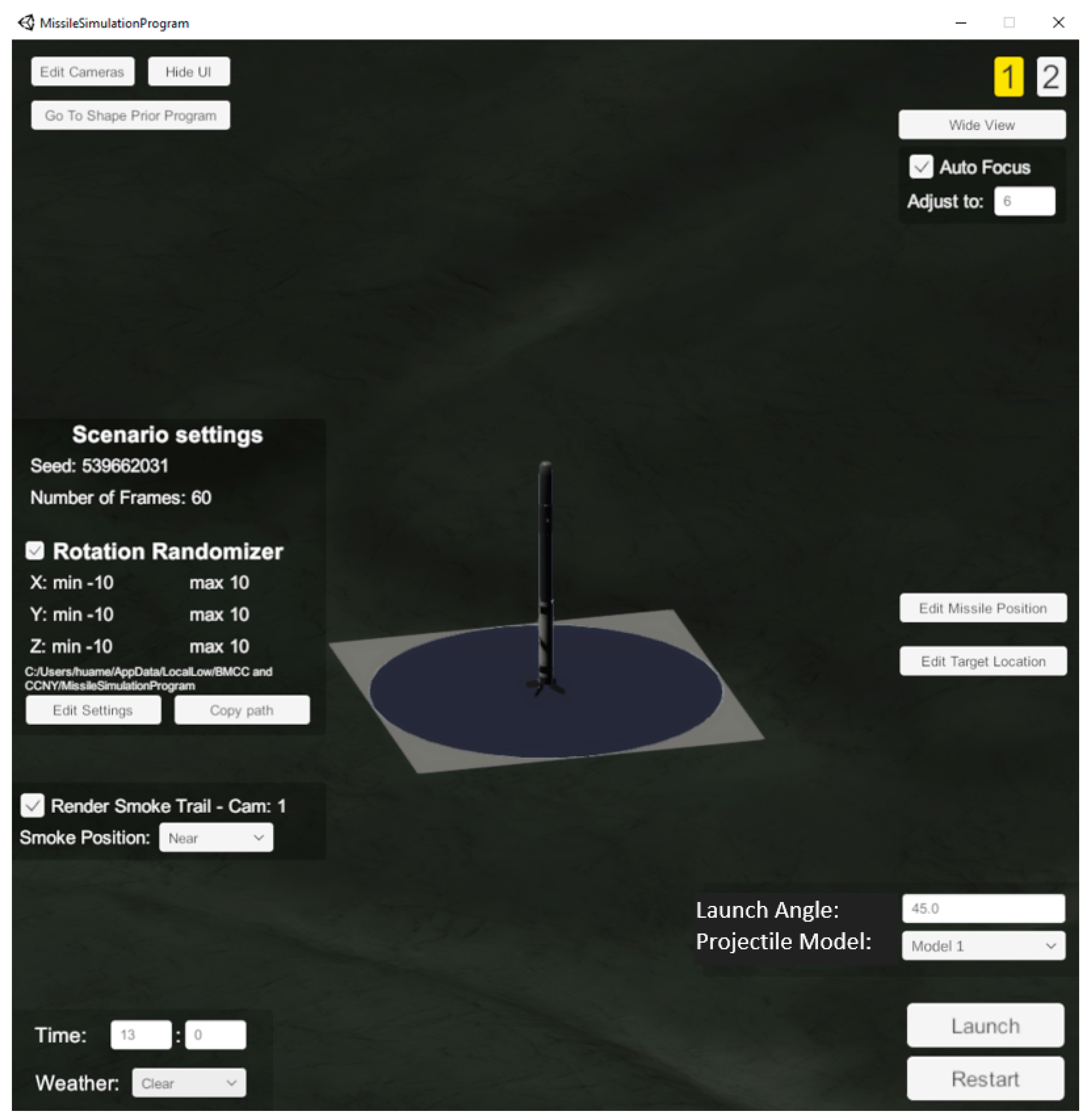
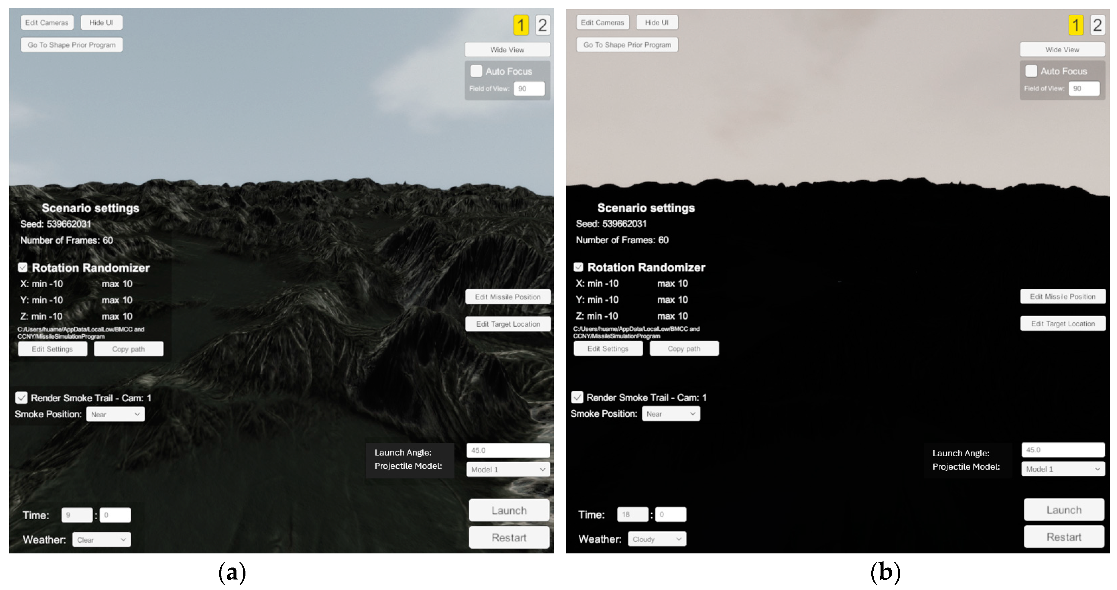
3. Synthetic Data Generation
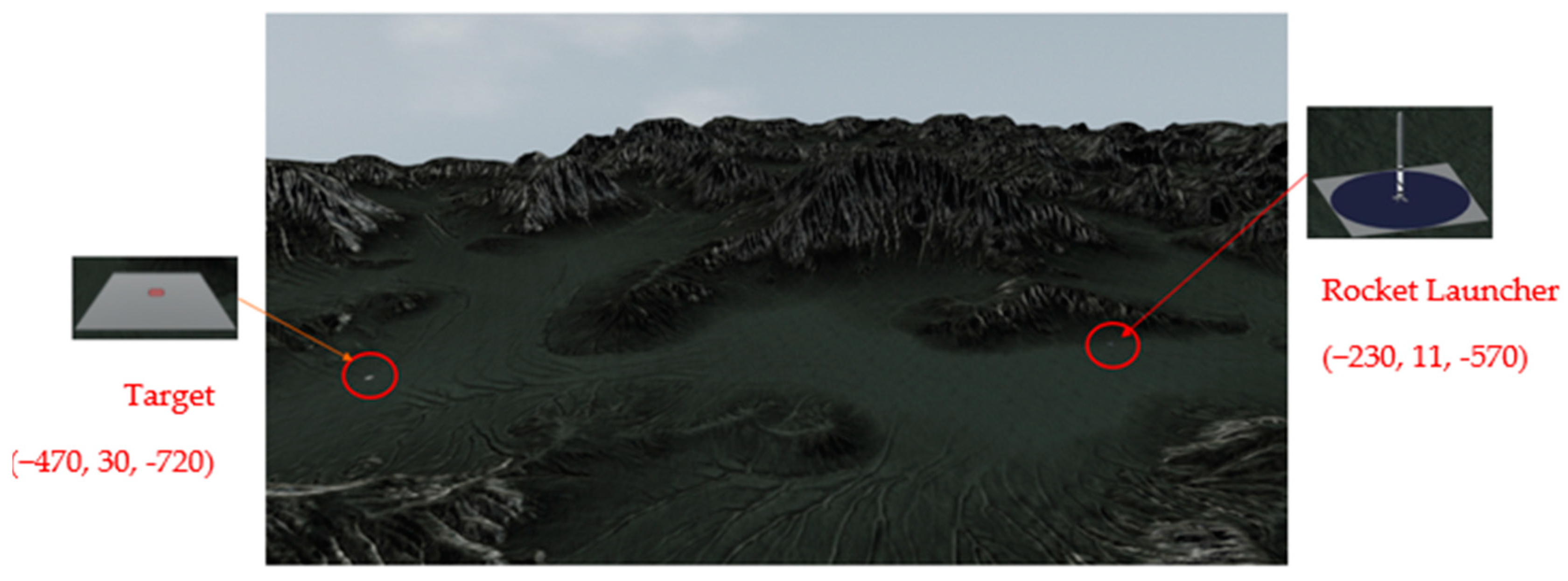
3.1. Background Models
3.2. 3D Projectile Models
3.3. Camera Models
3.4. Ground-Truth Annotation
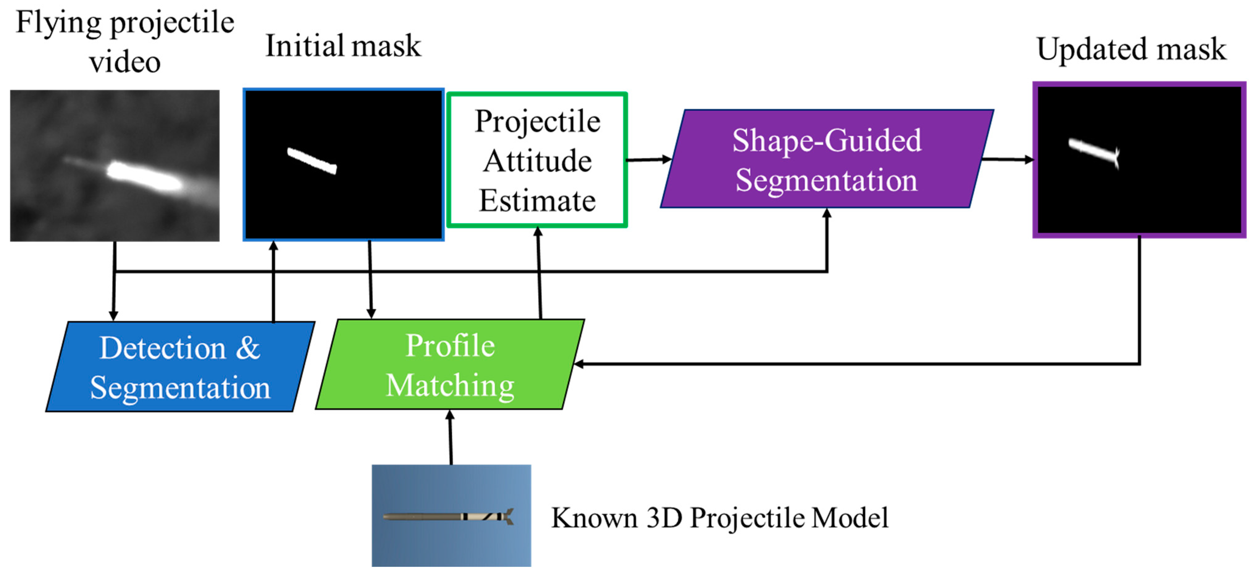
4. Approaches
4.1. Detection and Segmentation Module
4.2. Profile-Matching Module
4.2.1. Mask-Based Pose Estimation
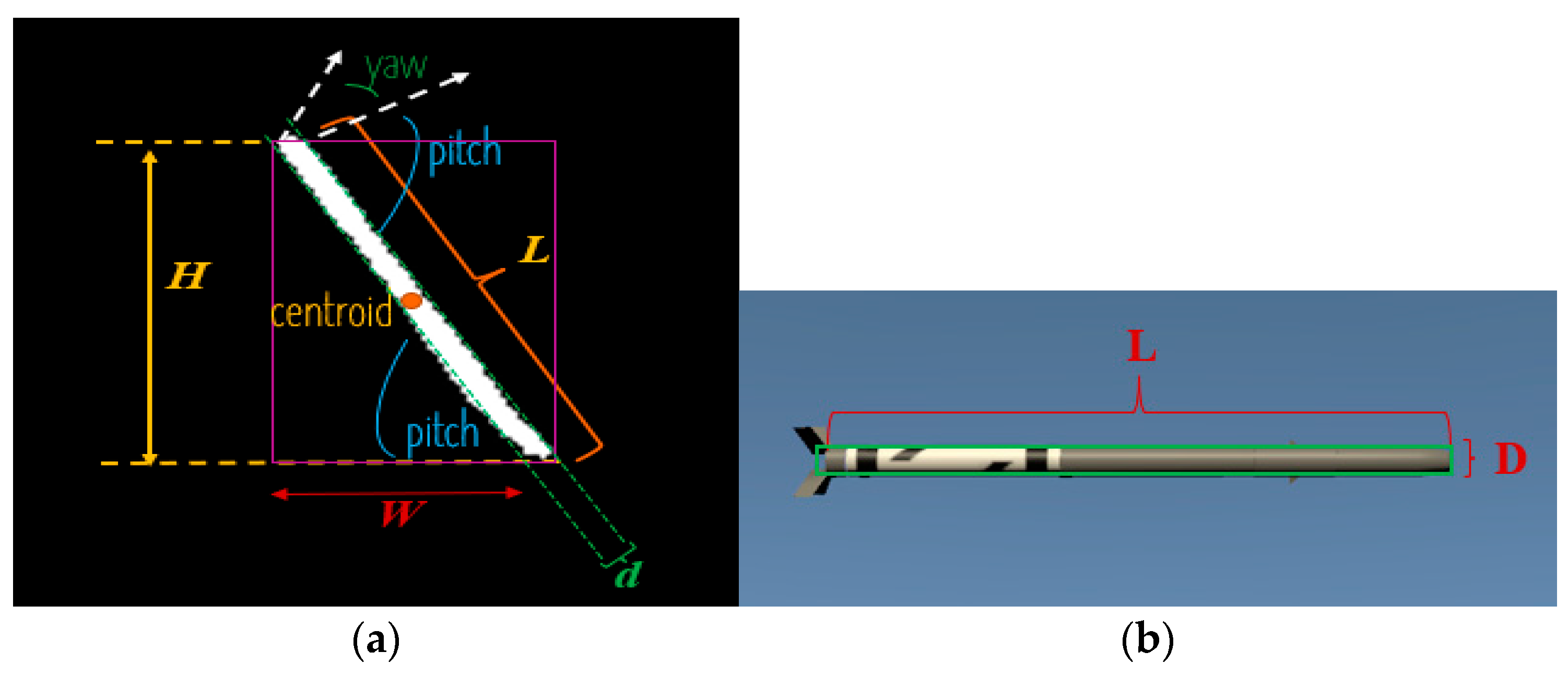
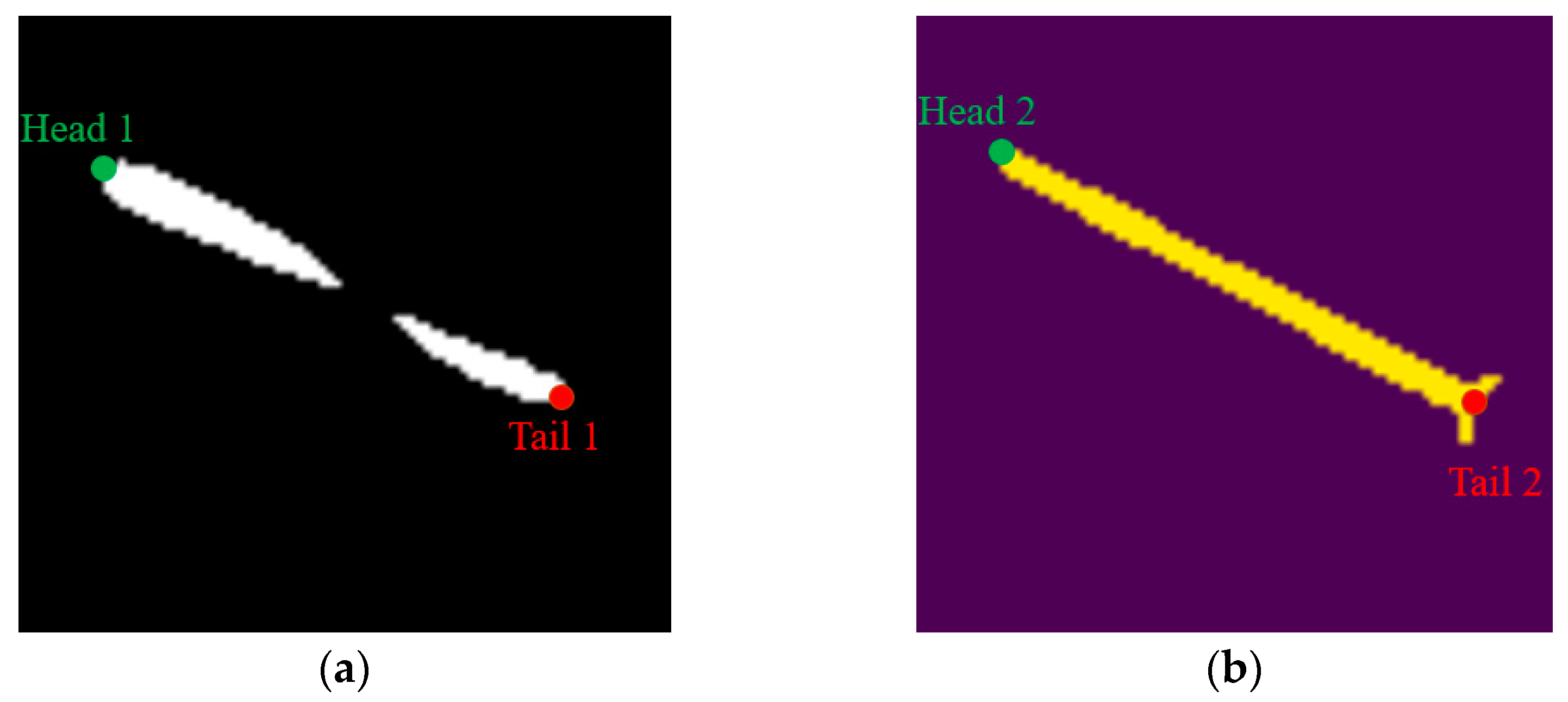
Pitch and Yaw Estimation
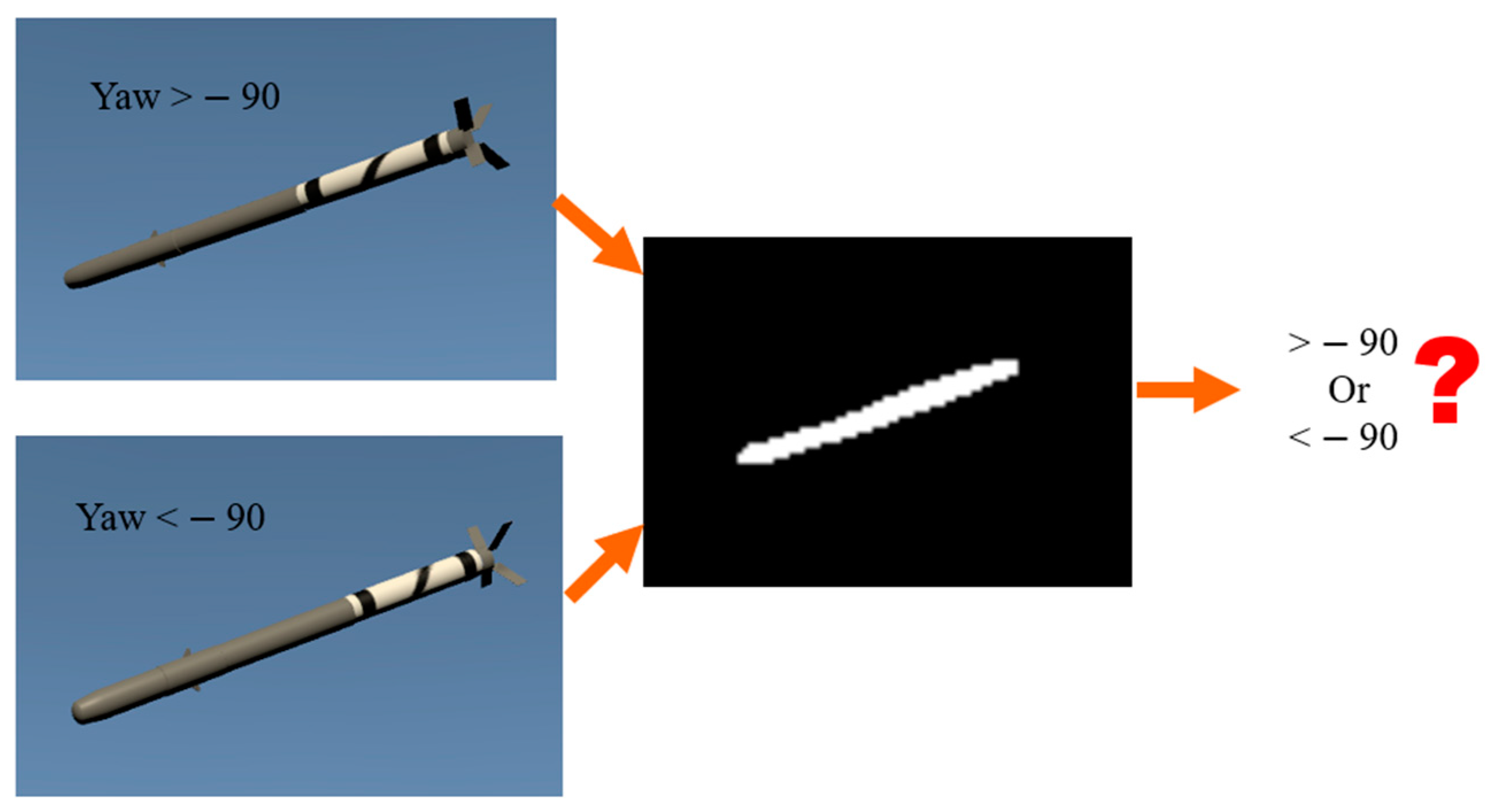
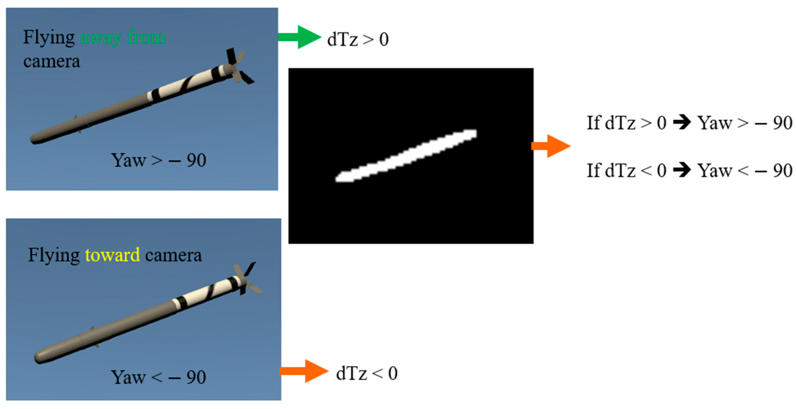
Ambiguity of Yaw Estimation
Estimation of Tx, Ty, and Tz
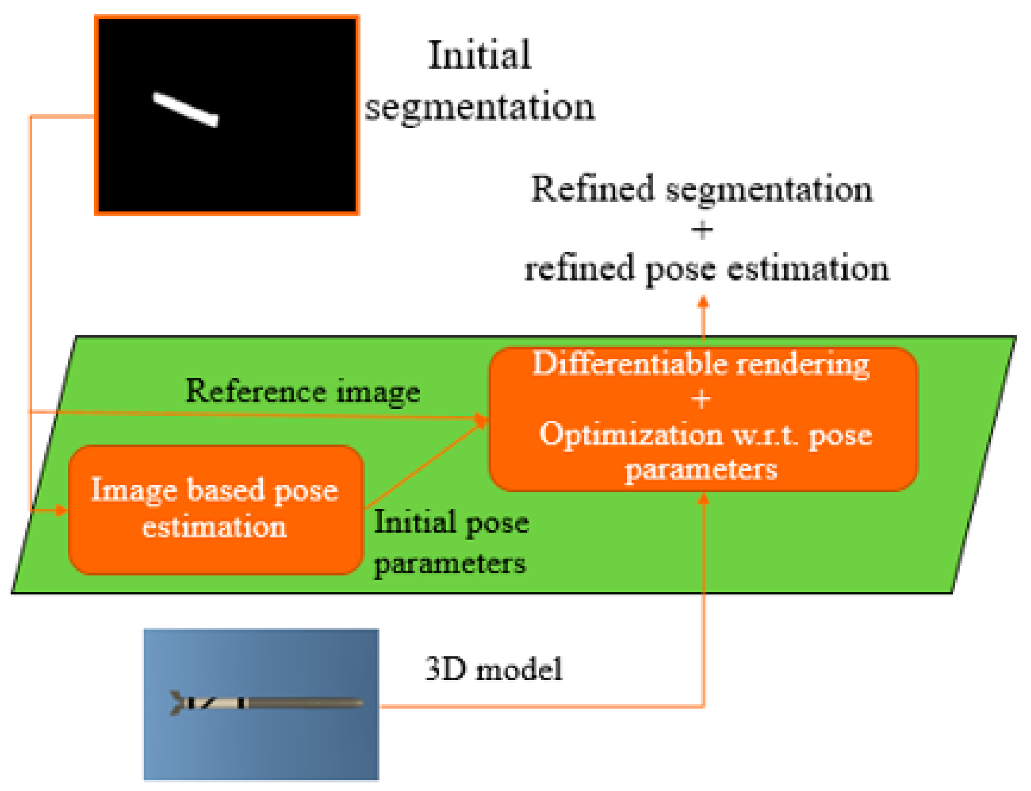
4.2.2. Pose Estimation through Profile Matching
4.3. Shape-Guided Segmentation
4.3.1. GVF-ASM
| Algorithm 1: GVF-ASM |
| Input: Target chip and a shape prior in the form of a binary mask. Output: Segmentation mask |
|
4.3.2. SIS-Cut
| Algorithm 2: SIS-Cut |
| Input: Target chip and a shape prior in the form of a binary mask. |
| Output: Segmentation mask |
|
| dist(pF,pB) = (7) |
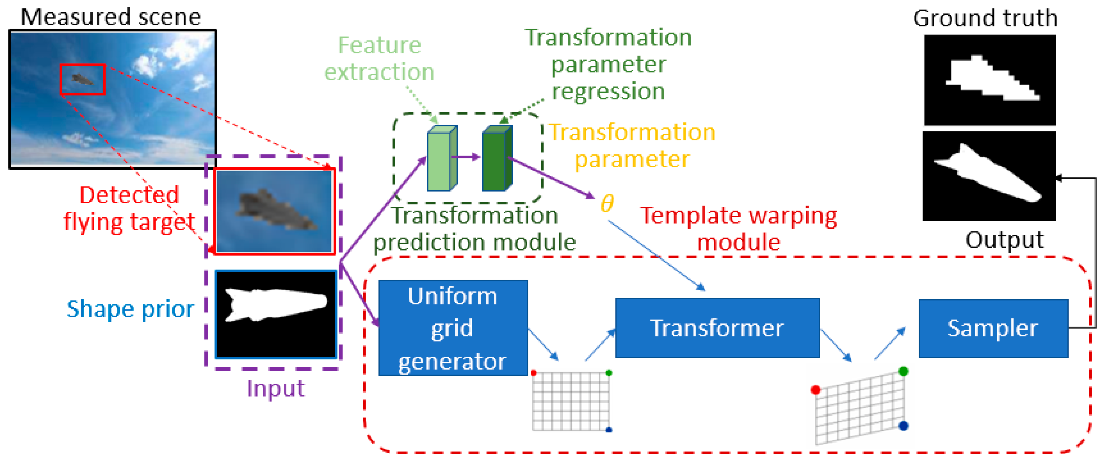
4.3.3. 2D TETRIS
Transformation Prediction Module
Template Warping Module
Shape Prior Generation
5. Experimental Procedures and Results
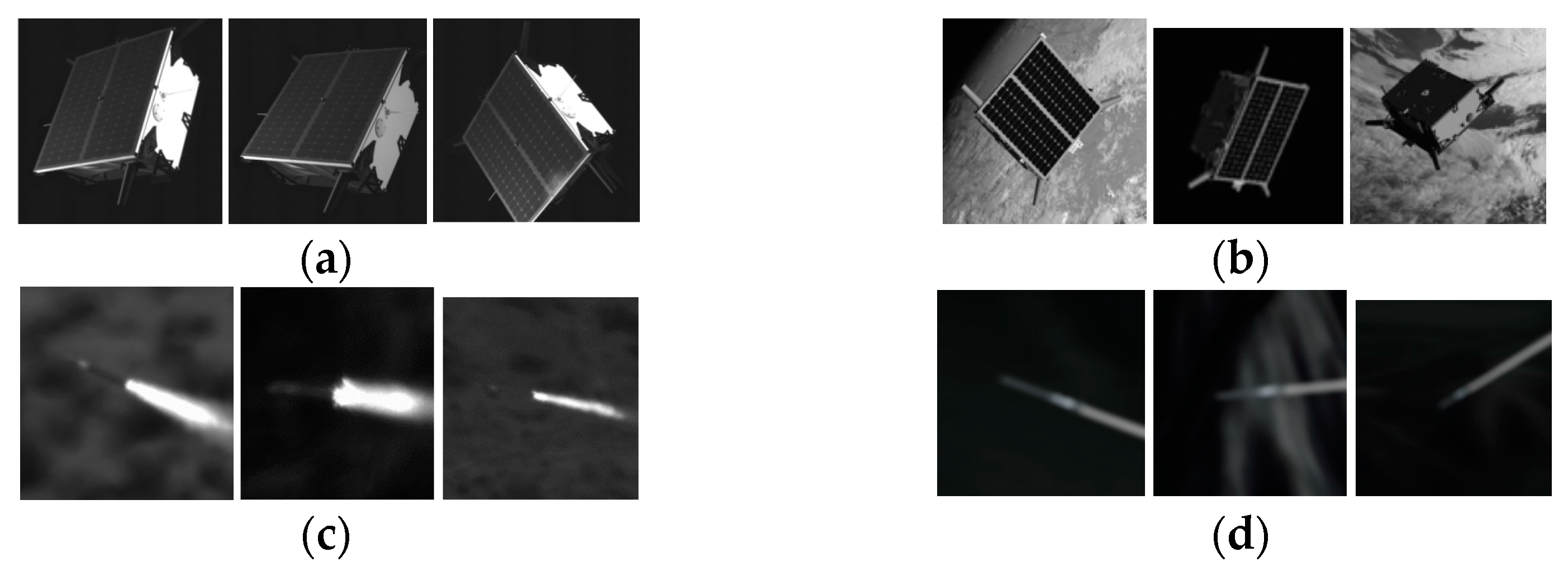
5.1. Datasets
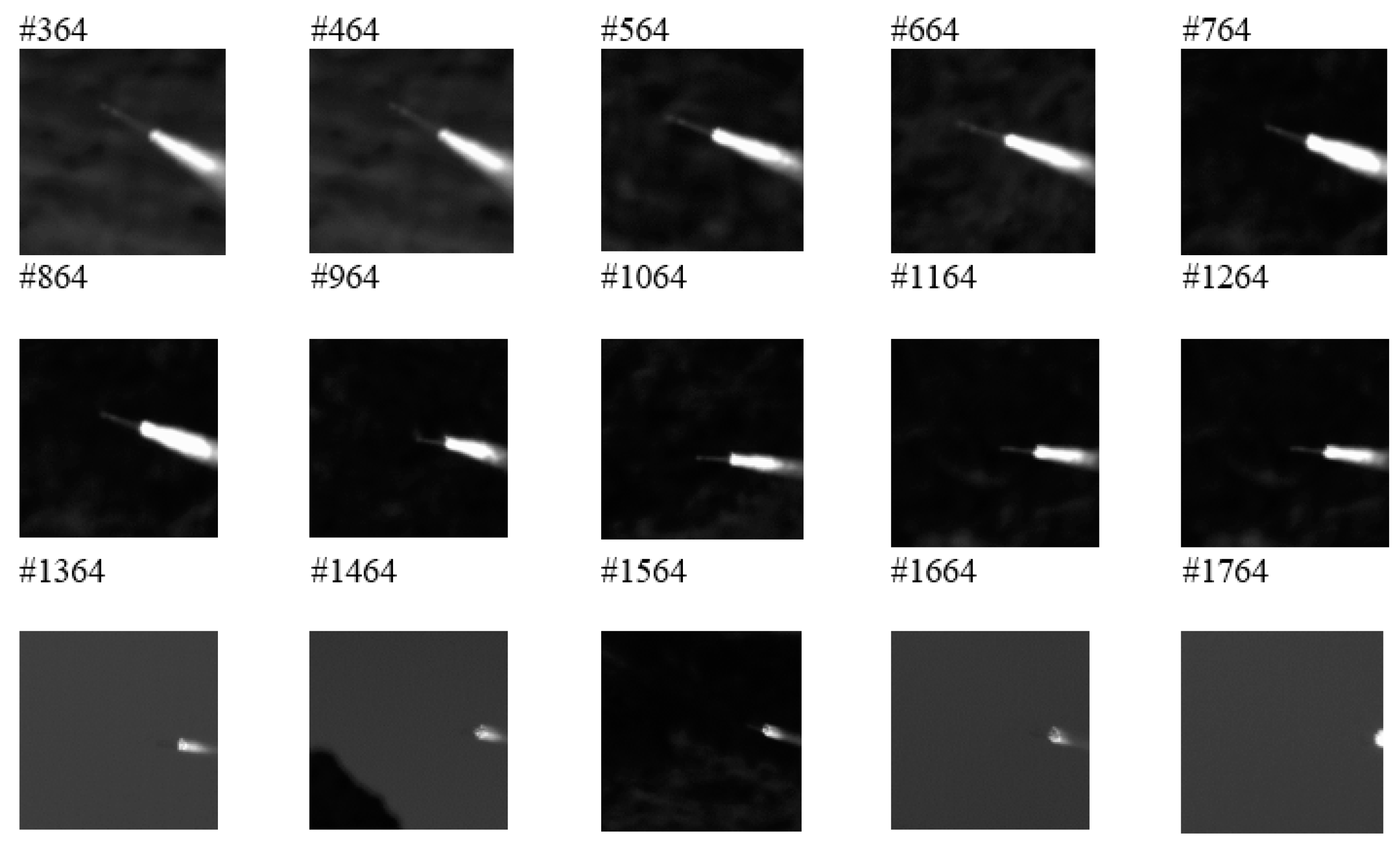
5.1.1. Simulated Data
5.1.2. Real Data
5.2. Mask R-CNN
5.2.1. Simulated Data
5.2.2. Real Data
5.3. Mask-Based Pose Estimation
5.3.1. Simulated Data
Unknown Tz
Known Tz
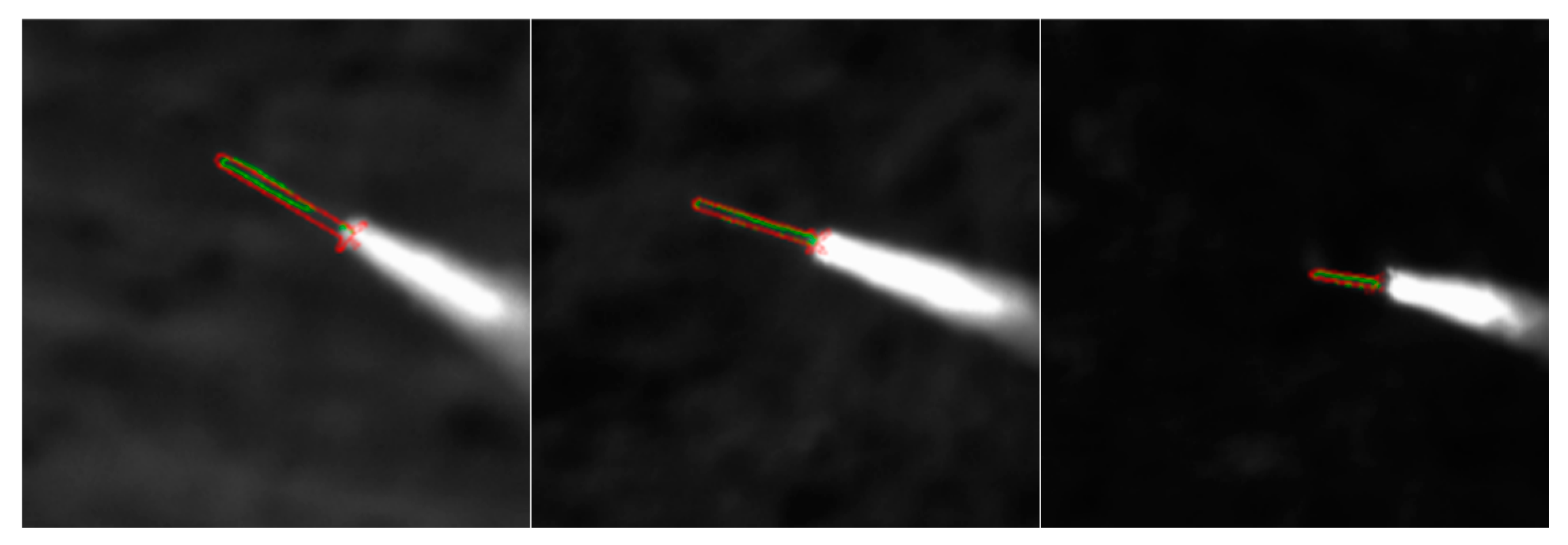
5.3.2. Real Data
5.4. Shape-Guided Segmentation
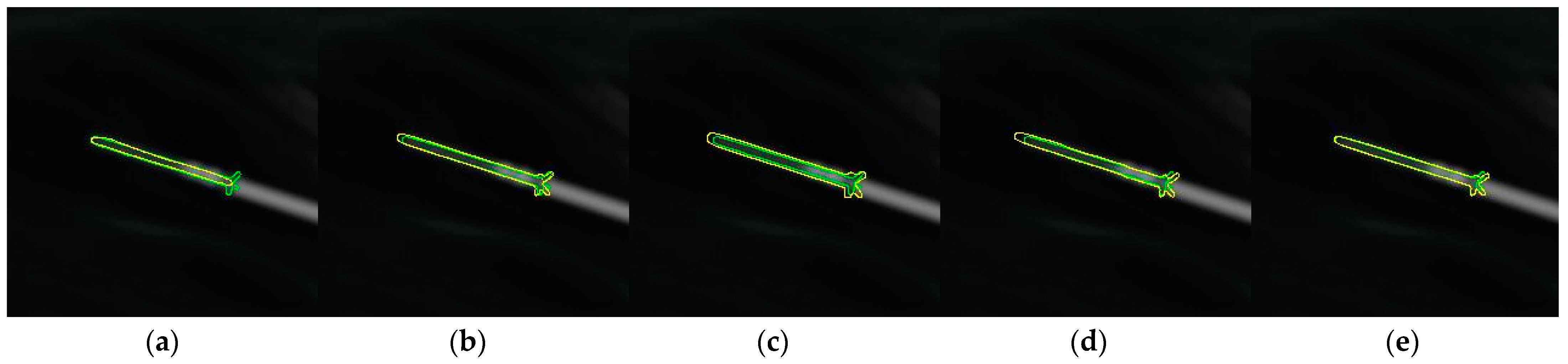
5.4.1. Simulated Data
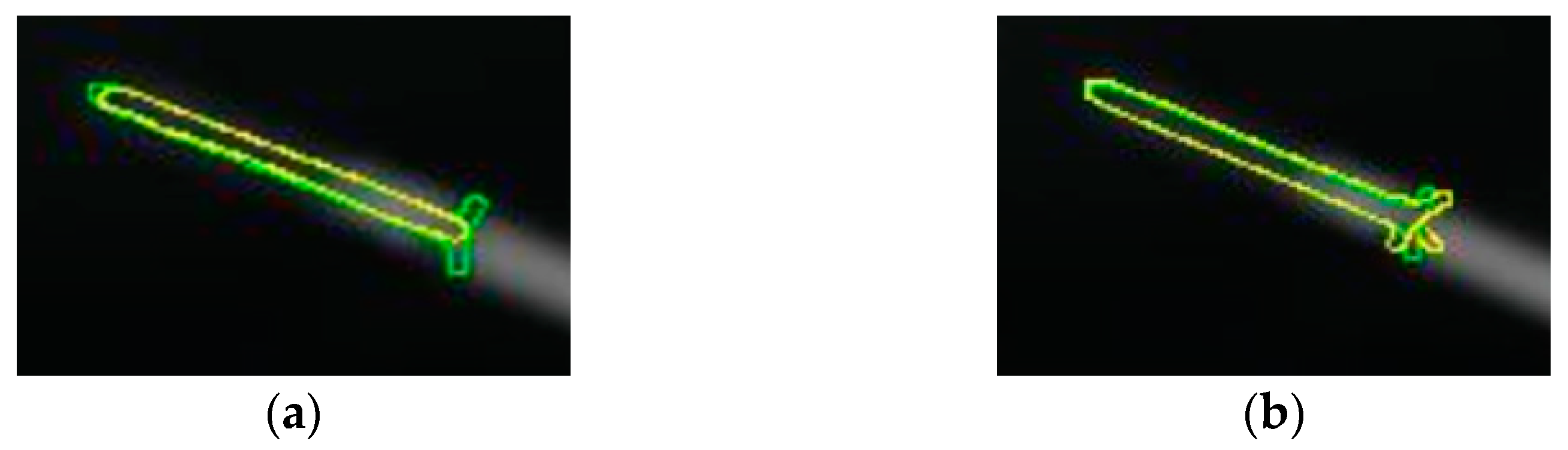
5.4.2. Real Data
5.5. Performance Evaluation
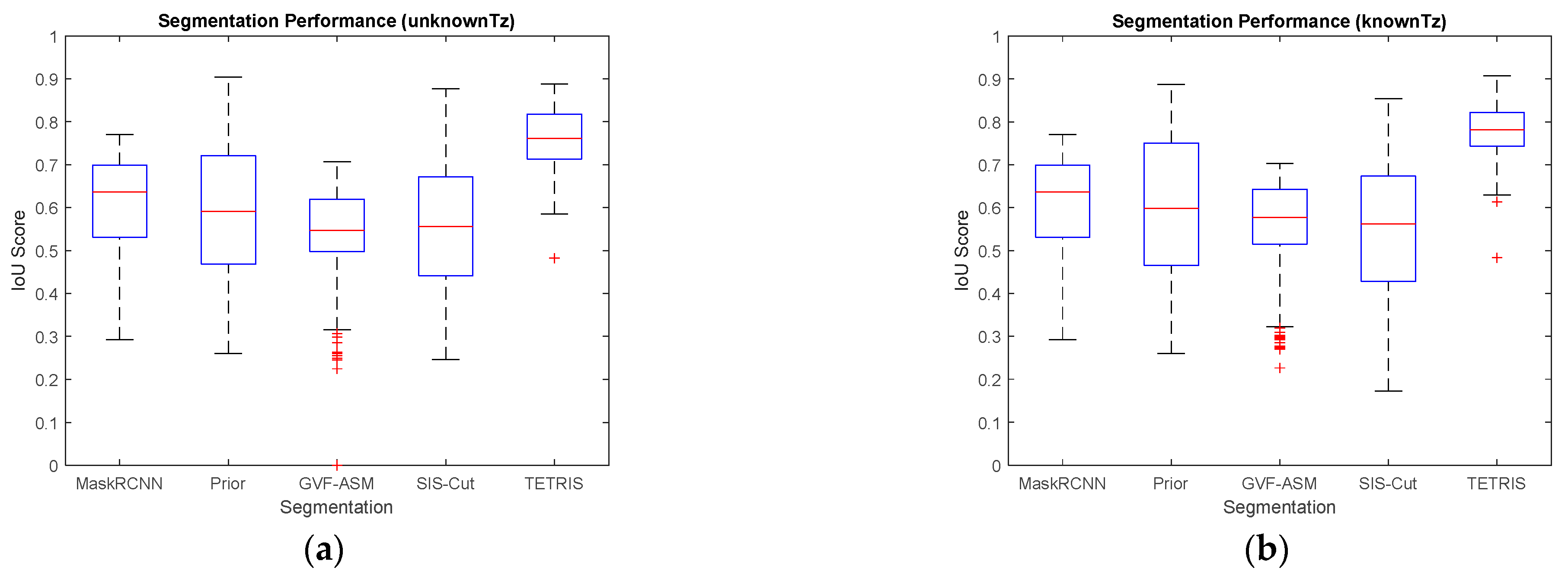
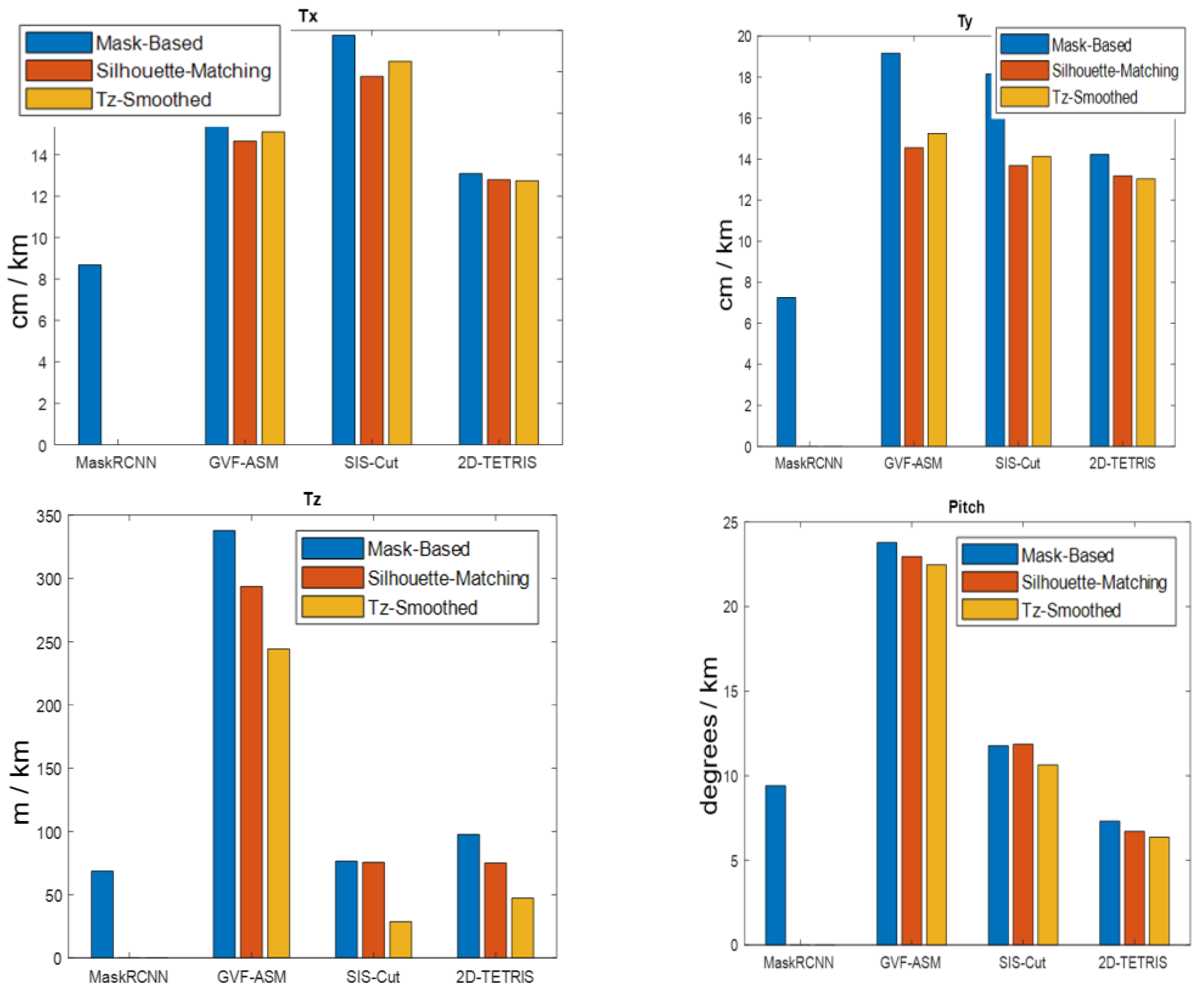
5.5.1. Unknown Tz
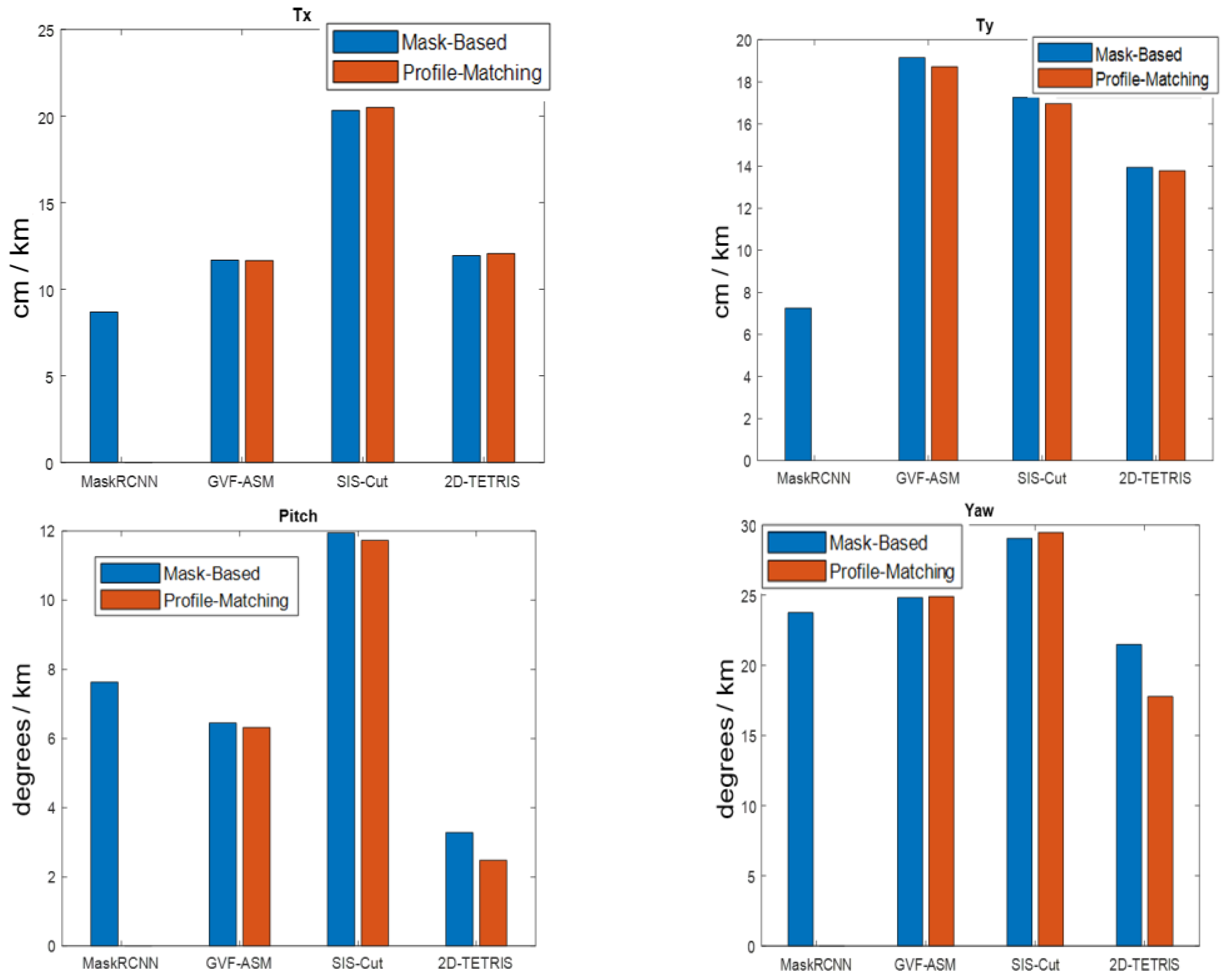
5.5.2. Known Tz
5.5.3. Runtime Comparison
6. Conclusions
Author Contributions
Funding
Institutional Review Board Statement
Informed Consent Statement
Data Availability Statement
Conflicts of Interest
References
- Hinterstoisser, S.; Holzer, S.; Cagniart, C.; Ilic, S.; Konolige, K.; Navab, N.; Lepetit, V. Multimodal templates for real-time detection of texture-less objects in heavily cluttered scenes. In Proceedings of the 2011 International Conference on Computer Vision (ICCV), Barcelona, Spain, 6–13 November 2011; IEEE: Piscataway, NJ, USA, 2011. [Google Scholar]
- Cao, Z.; Sheikh, Y.; Banerjee, N.K. Real-time scalable 6DOF pose estimation for textureless objects. In Proceedings of the 2016 IEEE International Conference on Robotics and Automation (ICRA), Stockholm, Sweden, 16–21 May 2016; IEEE: Piscataway, NJ, USA, 2016. [Google Scholar]
- Cootes, T.F.; Taylor, C.J.; Cooper, D.H.; Graham, J. Active shape models-their training and application. Comput. Vis. Image Underst. 1995, 61, 38–59. [Google Scholar] [CrossRef]
- Xu, C.; Prince, J.L. Gradient vector flow: A new external force for snakes. In Proceedings of the IEEE Computer Society Conference on Computer Vision and Pattern Recognition, San Juan, PR, USA, 17–19 June 1997; pp. 66–71. [Google Scholar]
- Boykov, Y.Y.; Jolly, M.-P. Interactive Graph Cuts for Optimal Bounday& Region Segmentation of Objects in N-D Images. In Proceedings of the Eighth IEEE International Conference on Computer Vision. ICCV 2001, Vancouver, BC, Canada, 7–14 July 2001. [Google Scholar]
- Lee MC, H.; Petersen, K.; Pawlowski, N.; Glocker, B.; Schaap, M. Tetris: Template transformer networks for image segmentation with shape priors. IEEE Trans. Med. Imaging 2019, 38, 2596–2606. [Google Scholar] [PubMed]
- Lee, A.; Dallmann, W.; Nykl, S.; Taylor, C.; Borghetti, B. Long-range pose estimation for aerial refueling approaches using deep neural networks. J. Aerosp. Inf. Syst. 2020, 17, 634–646. [Google Scholar] [CrossRef]
- Wang, Y.; Wang, H.; Liu, B.; Liu, Y.; Wu, J.; Lu, Z. A visual navigation framework for the aerial recovery of UAVs. IEEE Trans. Instrum. Meas. 2021, 70, 1–13. [Google Scholar] [CrossRef]
- Yang, J.; Wang, C.; Jiang, B.; Song, H.; Meng, Q. Visual perception enabled industry intelligence: State of the art, challenges and prospects. IEEE Trans. Ind. Inform. 2020, 17, 2204–2219. [Google Scholar] [CrossRef]
- Opromolla, R.; Fasano, G.; Rufino, G.; Grassi, M. A review of cooperative and uncooperative spacecraft pose determination techniques for close-proximity operations. Prog. Aerosp. Sci. 2017, 93, 53–72. [Google Scholar] [CrossRef]
- Sharma, S.; Park, T.H.; D’Amico, S. Spacecraft Pose Estimation Dataset (SPEED). Stanford Digital Repository. Available online: https://zenodo.org/records/6327547 (accessed on 21 December 2023).
- Zhu, M.; Derpanis, K.G.; Yang, Y.; Brahmbhatt, S.; Zhang, M.; Phillips, C.; Lecce, M.; Daniilidis, K. Single image 3D object detection and pose estimation for grasping. In Proceedings of the 2014 IEEE International Conference on Robotics and Automation (ICRA), Hong Kong, China, 31 May–7 June 2014; IEEE: Piscataway, NJ, USA, 2014. [Google Scholar]
- Marchand, E.; Hideaki, U.; Fabien, S. Pose estimation for augmented reality: A hands-on survey. IEEE Trans. Vis. Comput. Graph. 2015, 22, 2633–2651. [Google Scholar] [CrossRef] [PubMed]
- Yu, Y.K.; Wong, K.H.; Chang, M. Pose estimation for augmented reality applications using genetic algorithm. IEEE Trans. Syst. Man Cybern. Part B (Cybernetics) 2005, 35, 1295–1301. [Google Scholar] [CrossRef] [PubMed]
- Ferrara, P.; Piva, A.; Argenti, F.; Kusuno, J.; Niccolini, M.; Ragaglia, M.; Uccheddu, F. Wide-angle and long-range real time pose estimation: A comparison between monocular and stereo vision systems. J. Vis. Commun. Image Represent. 2017, 48, 159–168. [Google Scholar] [CrossRef]
- Kehl, W.; Milletari, F.; Tombari, F.; Ilic, S.; Navab, N. Deep learning of local rgb-d patches for 3d object detection and 6d pose estimation. In Proceedings of the European Conference on Computer Vision, Amsterdam, The Netherlands, 11–14 October 2016; Springer: Cham, Switzerland, 2016. [Google Scholar]
- Vidal, J.; Lin, C.-Y.; Marti, R. 6D pose estimation using an improved method based on point pair features. In Proceedings of the 2018 4th International Conference on Control, Automation and Robotics (Iccar), Auckland, New Zealand, 20–23 April 2018; IEEE: Piscataway, NJ, USA, 2018. [Google Scholar]
- Gao, Y.; Dai, Q. View-based 3D object retrieval: Challenges and approaches. IEEE Multimed. 2014, 21, 52–57. [Google Scholar] [CrossRef]
- Muja, M.; Rusu, R.B.; Bradski, G.; Lowe, D.G. Rein-a fast, robust, scalable recognition infrastructure. In Proceedings of the 2011 IEEE International Conference on Robotics and Automation, Shanghai, China, 9–13 May 2011; IEEE: Piscataway, NJ, USA, 2011. [Google Scholar]
- Hinterstoisser, S.; Cagniart, C.; Ilic, S.; Sturm, P.; Navab, N.; Fua, P.; Lepetit, V. Gradient response maps for real-time detection of textureless objects. IEEE Trans. Pattern Anal. Mach. Intell. 2011, 34, 876–888. [Google Scholar] [CrossRef] [PubMed]
- Gu, C.; Ren, X. Discriminative mixture-of-templates for viewpoint classification. In European Conference on Computer Vision; Springer: Berlin/Heidelberg, Germany, 2010. [Google Scholar]
- Sundermeyer, M.; Marton, Z.C.; Durner, M.; Brucker, M.; Triebel, R. Implicit 3d orientation learning for 6d object detection from rgb images. In Proceedings of the European Conference on Computer Vision (ECCV), Munich, Germany, 8–14 September 2018. [Google Scholar]
- Hodan, T.; Haluza, P.; Obdrzalek, S.; Matas, J.; Lourakis, M.; Zabulis, X. T-LESS: An RGB-D dataset for 6D pose estimation of texture-less objects. In Proceedings of the 2017 IEEE Winter Conference on Applications of Computer Vision (WACV), Santa Rosa, CA, USA, 24–31 March 2017; IEEE: Piscataway, NJ, USA, 2017. [Google Scholar]
- Lepetit, V.; Moreno-Noguer, F.; Fua, P. Epnp: An accurate o (n) solution to the pnp problem. Int. J. Comput. Vis. 2009, 81, 155–166. [Google Scholar] [CrossRef]
- Bleser, G.; Pastarmov, Y.; Stricker, D. Real-time 3d camera tracking for industrial augmented reality applications. In Proceedings of the 13th International Conference in Central Europe on Computer Graphics, Visualization and Computer Vision 2005 in Co-Operation with EUROGRAPHICS, Plzen, Czech Republic, January 31–February 4 2005. [Google Scholar]
- Petit, A.; Marchand, E.; Kanani, K. Vision-based detection and tracking for space navigation in a rendezvous context. In Int. Symp. on Artificial Intelligence, Robotics and Automation in Space; i-SAIRAS: Turin, Italy, 2012. [Google Scholar]
- Vacchetti, L.; Lepetit, V.; Fua, P. Combining edge and texture information for real-time accurate 3d camera tracking. In Proceedings of the Third IEEE and ACM International Symposium on Mixed and Augmented Reality, Arlington, VA, USA, 5 November 2004; IEEE: Piscataway, NJ, USA, 2004. [Google Scholar]
- Lowe, D.G. Distinctive image features from scale-invariant keypoints. Int. J. Comput. Vis. 2004, 60, 91–110. [Google Scholar] [CrossRef]
- Wagner, D.; Reitmayr, G.; Mulloni, A.; Drummond, T.; Schmalstieg, D. Pose tracking from natural features on mobile phones. In Proceedings of the 2008 7th IEEE/ACM International Symposium on Mixed and Augmented Reality, Cambridge, UK, 15–18 September 2008; IEEE: Piscataway, NJ, USA, 2008. [Google Scholar]
- Rad, M.; Lepetit, V. Bb8: A scalable, accurate, robust to partial occlusion method for predicting the 3d poses of challenging objects without using depth. In Proceedings of the IEEE International Conference on Computer Vision, Venice, Italy, 22–29 October 2017. [Google Scholar]
- Tekin, B.; Sinha, S.N.; Fua, P. Real-time seamless single shot 6d object pose prediction. In Proceedings of the IEEE Conference on Computer Vision and Pattern Recognition, Salt Lake City, UT, USA, 18–23 June 2018. [Google Scholar]
- Pavlakos, G.; Zhou, X.; Chan, A.; Derpanis, K.G.; Daniilidis, K. 6-dof object pose from semantic keypoints. In Proceedings of the 2017 IEEE International Conference on Robotics and Automation (ICRA), Singapore, 29 May–3 June 2017; IEEE: Piscataway, NJ, USA, 2017. [Google Scholar]
- Oberweger, M.; Rad, M.; Lepetit, V. Making deep heatmaps robust to partial occlusions for 3d object pose estimation. In Proceedings of the European Conference on Computer Vision (ECCV), Munich, Germany, 8–14 September 2018. [Google Scholar]
- Peng, S.; Liu, Y.; Huang, Q.; Zhou, X.; Bao, H. Pvnet: Pixel-wise voting network for 6dof pose estimation. In Proceedings of the IEEE/CVF Conference on Computer Vision and Pattern Recognition, Long Beach, CA, USA, 15–20 June 2019. [Google Scholar]
- Pham, T.; Cai, M.; Reid, I. Real-time monocular object instance 6d pose estimation. In Proceedings of the 29th British Machine Vision Conference (BMVC 2018), Newcastle, UK, 3 September–6 September 2019. [Google Scholar]
- Li, Y.; Wang, G.; Ji, X.; Xiang, Y.; Fox, D. Deepim: Deep iterative matching for 6d pose estimation. In Proceedings of the European Conference on Computer Vision (ECCV), Munich, Germany, 8–14 September 2018. [Google Scholar]
- Kehl, W.; Manhardt, F.; Tombari, F.; Ilic, S.; Navab, N. Ssd-6d: Making rgb-based 3d detection and 6d pose estimation great again. In Proceedings of the IEEE International Conference on Computer Vision, Venice, Italy, 22–29 October 2017. [Google Scholar]
- Xiang, Y.; Schmidt, T.; Narayanan, V.; Fox, D. Posecnn: A convolutional neural network for 6d object pose estimation in cluttered scenes. arXiv 2017, arXiv:1711.00199. [Google Scholar]
- Li, X.; Chen, G.; Blasch, E.; Pham, K. Detecting missile-like flying target from a distance in sequence images. In Signal Processing, Sensor Fusion, and Target Recognition XVII; SPIE: Paris, France, 2008; Volume 6968. [Google Scholar]
- He, K.; Gkioxari, G.; Dollár, P.; Girshick, R. Mask r-cnn. In Proceedings of the IEEE International Conference on Computer Vision, Venice, Italy, 22–29 October 2017. [Google Scholar]
- PyTorch3D. Available online: https://pytorch3d.readthedocs.io/en/latest/overview.html# (accessed on 21 December 2023).
- Grosgeorge, D.; Petitjean, C.; Dacher, J.-N.; Ruan, S. Graph cut segmentation with a statistical shape model in cardiac MRI. Comput. Vis. Image Underst. 2013, 117, 1027–1035. [Google Scholar] [CrossRef]
- Cha, J.; Farhangi, M.M.; Dunlap, N.; Amini, A.A. Segmentation and tracking of lung nodules via graph-cuts incorporating shape prior and motion from 4D CT. Med. Phys. 2018, 45, 297–306. [Google Scholar] [CrossRef] [PubMed]
- Jaderberg, M.; Simonyan, K.; Zisserman, A. Spatial transformer networks. In Advances in Neural Information Processing Systems; MIT Press: Cambridge, MA, USA, 2015; Volume 28. [Google Scholar]
- Simonyan, K.; Zisserman, A. Very deep convolutional networks for large-scale image recognition. arXiv 2014, arXiv:1409.1556. [Google Scholar]
- He, K.; Zhang, X.; Ren, S.; Sun, J. Deep residual learning for image recognition. In Proceedings of the IEEE Conference on Computer Vision and Pattern Recognition, Salt Lake City, UT, USA, 18–23 June 2016. [Google Scholar]
- Szegedy, C.; Liu, W.; Jia, Y.; Sermanet, P.; Reed, S.; Anguelov, D.; Erhan, D.; Vanhoucke, V.; Rabinovich, A. Going deeper with convolutions. In Proceedings of the IEEE Conference on Computer Vision and Pattern Recognition, Boston, MA, USA, 7–12 June 2015. [Google Scholar]
- Szegedy, C.; Vanhoucke, V.; Ioffe, S.; Shlens, J.; Wojna, Z. Rethinking the inception architecture for computer vision. In Proceedings of the IEEE Conference on Computer Vision and Pattern Recognition, Las Vegas, NV, USA, 7–30 June 2016. [Google Scholar]
- Szegedy, C.; Ioffe, S.; Vanhoucke, V.; Alemi, A. Inception-v4, inception-resnet and the impact of residual connections on learning. In Proceedings of the Thirty-first AAAI Conference on Artificial Intelligence, Vancouver, BC, Canada, 20–27 February 2017. [Google Scholar]
- Wu, Y.; Kirillov, A.; Massa Francisco Lo, W.-Y.; Girshick, R. Detectron2. 2019. Available online: https://github.com/facebookresearch/detectron2 (accessed on 21 December 2023).


| Train | Validation | Test | |
|---|---|---|---|
| Launch Angle | 40 | 41 | 39 |
| Time of the day | 17:00 | 17:30 | 17:15 |
| Random seed | 539662031 | 539662032 | 539662033 |
| Weather | Cloudy | Cloudy | Cloudy |
| Camera | 1 | 1 | 1 |
| # of frames | 175 | 175 | 175 |
| GVF-ASM | GraphCut Criterion-Based | 2D TETRIS | |
|---|---|---|---|
| Time | 1502 (s) | 995 (s) | 7.12 (s) |
| Framerate (ratio) | ~0.12 fps (1) | ~0.18 fps (1.5) | ~25 fps (208) |
| Code | MatlabTM | MatlabTM | Python |
| OS | Windows 10 | Windows 10 | Ubuntu 20.04 |
| Hardware | CPU | CPU | CPU + GPU |
Disclaimer/Publisher’s Note: The statements, opinions and data contained in all publications are solely those of the individual author(s) and contributor(s) and not of MDPI and/or the editor(s). MDPI and/or the editor(s) disclaim responsibility for any injury to people or property resulting from any ideas, methods, instructions or products referred to in the content. |
© 2024 by the authors. Licensee MDPI, Basel, Switzerland. This article is an open access article distributed under the terms and conditions of the Creative Commons Attribution (CC BY) license (https://creativecommons.org/licenses/by/4.0/).
Share and Cite
Chen, H.; Zhu, Z.; Tang, H.; Blasch, E.; Pham, K.D.; Chen, G. Flying Projectile Attitude Determination from Ground-Based Monocular Imagery with a Priori Knowledge. Information 2024, 15, 201. https://doi.org/10.3390/info15040201
Chen H, Zhu Z, Tang H, Blasch E, Pham KD, Chen G. Flying Projectile Attitude Determination from Ground-Based Monocular Imagery with a Priori Knowledge. Information. 2024; 15(4):201. https://doi.org/10.3390/info15040201
Chicago/Turabian StyleChen, Huamei, Zhigang Zhu, Hao Tang, Erik Blasch, Khanh D. Pham, and Genshe Chen. 2024. "Flying Projectile Attitude Determination from Ground-Based Monocular Imagery with a Priori Knowledge" Information 15, no. 4: 201. https://doi.org/10.3390/info15040201
APA StyleChen, H., Zhu, Z., Tang, H., Blasch, E., Pham, K. D., & Chen, G. (2024). Flying Projectile Attitude Determination from Ground-Based Monocular Imagery with a Priori Knowledge. Information, 15(4), 201. https://doi.org/10.3390/info15040201