Abstract
With the vast amount of social media posts available online, topic modeling and sentiment analysis have become central methods to better understand and analyze online behavior and opinion. However, semantic and sentiment analysis have rarely been combined for joint topic-sentiment modeling which yields semantic topics associated with sentiments. Recent breakthroughs in natural language processing have also not been leveraged for joint topic-sentiment modeling so far. Inspired by these advancements, this paper presents a novel framework for joint topic-sentiment modeling of short texts based on pre-trained language models and a clustering approach. The method leverages techniques from dimensionality reduction and clustering for which multiple algorithms were considered. All configurations were experimentally compared against existing joint topic-sentiment models and an independent sequential baseline. Our framework produced clusters with semantic topic quality scores of up to while the best score among the previous approaches was . The sentiment classification accuracy increased from to and the uniformity of sentiments within the clusters reached up to in contrast to the baseline of . The presented approach can benefit various research areas such as disaster management where sentiments associated with topics can provide practical useful information.
1. Introduction
“What people think” has historically been an important piece of information during many decision-making processes [1]. With the rise of social media platforms, an increasing amount of information on exactly such thoughts has become available to the public [2]. To extract meaningful information from the myriad of posts at hand, computational methods such as topic modeling [3,4] and sentiment analysis [1,2,5] have been researched and adapted specifically for short-form textual social media data. In practice, this allows for the analysis and monitoring of a variety of real-world phenomena such as earthquakes [6,7], floodings [8,9], refugee movements [10] or disease outbreaks [11,12,13] through social media data.
Traditionally, semantic analysis in the form of topic modeling and sentiment analysis has mostly been conducted separately, resulting in sequential workflows that use the two modalities in different ways. Apart from a few joint topic-sentiment models (e.g., [14,15,16]) based on the classic topic modeling technique Latent Dirichlet Allocation (LDA) [17], the joint analysis of these two features has previously not received much attention. However, sentiments can provide additional information about semantic topics that might be helpful for critical events such as natural disasters [18]. This situation is especially remarkable as traditional topic modeling has undergone an evolution introducing pre-trained Large Language Models (LLMs) into their working principles in recent years. Specifically, research has shown that a technique based on the clustering of embedding vectors can outperform classic topic modeling methods such as LDA [19,20,21]. Yet, extensions of this framework, have hardly been considered so far.
Given these developments, this research study introduces a novel approach to joint topic-sentiment modeling called the Joint Topic-Sentiment (JTS) framework. It is capable of computing semantic clusters of topics that are associated with a sentiment. The approach works by clustering joint feature vectors that represent both the semantic meaning and the sentiment of each input document. As it leverages distinct components for semantic embedding creation, dimensionality reduction, and clustering, the JTS framework itself allows for a degree of flexibility. Components can be exchanged depending on the needs of the user, e.g., if the data are multilingual or monolingual or if certain runtime requirements should be met. We realized the JTS framework using Principal Component Analysis (PCA) and Uniform Manifold Approximation and Projection (UMAP) for dimensionality reduction and k-means, a Growing Self-Organizing Map (GSOM) and Hierarchical Density-Based Spatial Clustering of Applications with Noise (HDBSCAN) for clustering. The respective variants were compared against each other and previous approaches for joint topic-sentiment modeling. Additionally, a sequential, independent topic modeling plus sentiment classification approach using BERTopic (s. Section 3) was considered for comparison. Our JTS framework achieved a topic coherence score of up to and a topic diversity score of up to whereas the highest respective scores among all other approaches were and . Simultaneously, the sentiment classification accuracy improved from , which was the best value among the existing joint topic-sentiment models, to with our approach. The uniformity of sentiments within the clusters reached up to compared to of the independent BERTopic plus sentiment classification approach. The key contributions of our research are therefore as follows:
- We introduce the novel JTS framework for joint topic-sentiment modeling which uses LLMs and a clustering approach.
- Our framework was evaluated using different configurations and compared against previous approaches as well as an independent, sequential approach.
- The results indicate that the JTS framework is capable of producing more coherent clusters of social media posts both concerning semantics and sentiments while simultaneously providing the highest sentiment classification accuracy.
Going further, our study adheres to the following structure. First, in Section 2, the related work regarding topic modeling, sentiment classification, and joint-topic-sentiment modeling is summarized. In Section 3, we present the architecture, working principles, and implementation of our JTS framework. Moreover, the experimental setup and the evaluation metrics are explained. We then present our results in Section 4. This is followed by a discussion of the results and the methodology in Section 5. Finally, the contributions of our study are summarized in Section 6.
2. Related Work
The paper draws from advancements in sentiment classification and topic modeling which are reviewed in this section. Additionally, recent works in joint topic-sentiment modeling are examined.
2.1. Topic Modeling
The presented JTS framework extracts semantic topics associated with sentiments from large collections of texts. It is, therefore, closely related to classic topic modeling, which is a technique for topic discovery in collections of documents. Formally, topic modeling can be viewed as a form of content analysis or an unsupervised categorization task where one or more topic codes are assigned to each document [22]. Topic modeling has been used and developed further in many different fields including computer science, computational linguistics, geographic information science, social sciences, and humanities [7,23,24,25,26,27]. Early techniques for topic modeling include Latent Semantic Analysis (LSA) [28], Probabilistic Latent Semantic Analysis (PLSA) [29] and Non-negative Matrix Factorization (NMF) [30] which are probabilistic techniques based on word co-occurrences. A major milestone in the field was the introduction of LDA by [17] which still is one of the most widely used topic models until today. The model parameters used for topic assignment can be inferred using variational techniques [17], Gibb’s sampling [31] or using Variational Autoencoders (VAEs) [32]. Notably, LDA has been widely adapted to include a variety of characteristics such as time, space, or social media users [33,34].
With the evolution of natural language processing techniques, especially word and paragraph embeddings [35,36], LDA has been adapted to include semantic embedding information leading to the Embedded Topic Model (ETM) by Dieng et al. [37]. Simultaneously, a novel approach to topic modeling based on the clustering of such embedding vectors has emerged. The idea was first proposed by Sia et al. [19] who showed that clustering high-dimensional semantic embedding vectors can be a powerful strategy for topic modeling which performed similarly to LDA. The idea was refined by Angelov [20] who proposed top2vec as a standalone topic model. Its underlying rationale is the assumption that the semantic embedding space generated by doc2vec is a continuous representation of topics. It, therefore, makes sense to cluster document embeddings in this semantic space to retrieve discrete topics. Grootendorst [21] extended this idea with the introduction of BERTopic which uses state-of-the-art Sentence-BERT (SBERT) embeddings and a class-based term frequency and inverse document frequency (tf-idf) procedure for extracting topic-defining words.
A comprehensive comparison of those previous probabilistic and clustering-based topic modeling methods was conducted by Grootendorst [21]. The results are summarised in Table 1 and include three data sets: 20 Newsgroups [38], BBC News [39] and Trump’s Tweets [21]. top2vec and BERTopic by far outperformed LDA and NMF in terms of topic coherence measured by the Normalized Pointwise Mutual Information (NPMI) and Topic Diversity (TD).

Table 1.
Quantitative comparison of previous probabilistic and clustering-based topic models. The highest respective values for each data set and metric are highlighted in bold.
2.2. Sentiment Classification
Alongside the increasing presence and availability of opinionated content such as social media posts and personal blogs, understanding and analyzing people’s opinions toward a particular topic has become a distinct research area called sentiment analysis [1,5]. Focusing primarily on natural language processing, studies usually classify opinions into predefined categories such as negative/positive [40] or negative/neutral/positive [41]. Sentiment classification can occur on a document level, sentence level, or concerning particular aspects of the content. The main approaches for sentiment classification can generally be divided into three categories: (1) lexicon-based techniques which rely on pre-defined dictionaries of words or phrases associated with sentiment scores, (2) machine-learning methods relying on models such Support Vector Machines (SVMs) or random forests for supervised learning and (3) deep learning methods relying on recurrent, Long Short-Term Memory (LSTM) or transformer-architecture neural networks [2]. For sentiment analysis of short-form textual content, models based on pre-trained transformer networks such as Bidirectional Encoder Representations from Transformer (BERT) outperformed previous methods, especially when evaluated on tweets [42]. Table 2 depicts the mean recall of different models for sentiment classification on the English-language TweetEval data set [43] based on the study of Loureiro et al. [44]. The base Robustly Optimized BERT Approach (RoBERTa) model [45] as well as Twitter-RoBERTa pre-trained on a large corpus of tweets [44] achieved significantly higher values.
Table 2.
Mean recall for different classification models on the TweetEval test data set for sentiment analysis. The best score is highlighted in bold.
BERT-based models can also be pre-trained on multiple languages, allowing for high performance for multilingual learning tasks including sentiment classification. Table 3 shows the F1 scores for sentiment classification tasks in different languages as in the work of Barbieri et al. [42]. The multilingual XLM-RoBERTa [46] and Twitter-XLM-RoBERTa models fine-tuned with monolingual data greatly outperformed FastText [47] in the respective languages.
Table 3.
F1 scores for sentiment classification tasks in different languages based on the work of Barbieri et al. [42]. The highest value for each language is highlighted in bold.
Concerning social media analysis, the results of a sentiment classification algorithm might be input to further processing. To provide some examples, Camacho et al. [48] combined sentiment analysis with spatial clustering and statistics to examine geocoded tweets. Paul et al. [49] conducted a spatiotemporal sentiment analysis of tweets concerning the 2016 US presidential election and Kovacs-Györi et al. [50] leveraged sentiment analysis and spatiotemporal analysis to extract spatial and temporal patterns of park visits.
2.3. Joint Topic-Sentiment Modeling
While the individual fields of topic modeling and sentiment analysis have undergone several evolutions in recent years, the underlying techniques primarily focus on analyzing topics or sentiments separately from each other. Classic topic models do not output sentiment information which might provide the user with another level of knowledge and sentiment classification models deliver no context of what the posts are actually about. For this reason, a small number of joint topic-sentiment models have been developed, most of which can be considered an extension of LDA. The first major contribution to this research strand has been made by Lin and He [14] who introduced the Joint Sentiment/Topic (JST) model which follows an altered LDA architecture that includes an additional sentiment layer. Consequently, topics are associated with sentiment labels, and words with both sentiment labels and topics. Lin et al. [51] also presented Reverse-JST which reverses the sequence of sentiment and topic generation in the modeling process. The inference mechanism of JST relies on word co-occurrences. To circumvent the shortcomings of the bag-of-words-based approach (e.g., if the corpus is small) Fu et al. [15] additionally included word embeddings (e.g., word2vec or FastText) in the model resulting in the Topic-Sentiment Joint Model with Word Embeddings (TSWE). It extends the conditioned probability distribution of words given topics and sentiments in the JST model with a word embedding component. Dermouche et al. [16] introduced a topic-sentiment model similar to JST, which, however, can produce different descriptions of topics based on the different sentiment polarities and computes a topic-specific sentiment distribution. Liang et al. [52] adapted the JST approach for online reviews and ratings.
The main shortcoming of the above approaches is that the inferred sentiments do not have a direct meaning such as “negative” “neutral” or “positive”. Although paradigm words can be injected to provide the model with a sense of orientation [14], the lexicon has to be curated by hand and the inference mechanism uses a bag-of-words approach. This makes the above methods not nearly as reliable in comparison to newer neural network-based sentiment classification methods, e.g., [53,54], and renders the results hard to interpret if more than two classes are used. Moreover, a systematic comparison of the existing joint topic-sentiment topic models has not been conducted yet. Throughout previous works, the data sets and metrics used for the evaluation often differ vastly, as is the case for [14,15,16]. In the study of Fu et al. [15], TSWE generally outperformed JST in terms of the Normalized Mutual Information (NMI) of the extracted topics and regarding the sentiment classification accuracy, though no tabular data are available for the latter. For TSWE, the NMI ranged from to for two test data sets and different numbers of topics. JST only reached values between and .
3. Materials & Methods
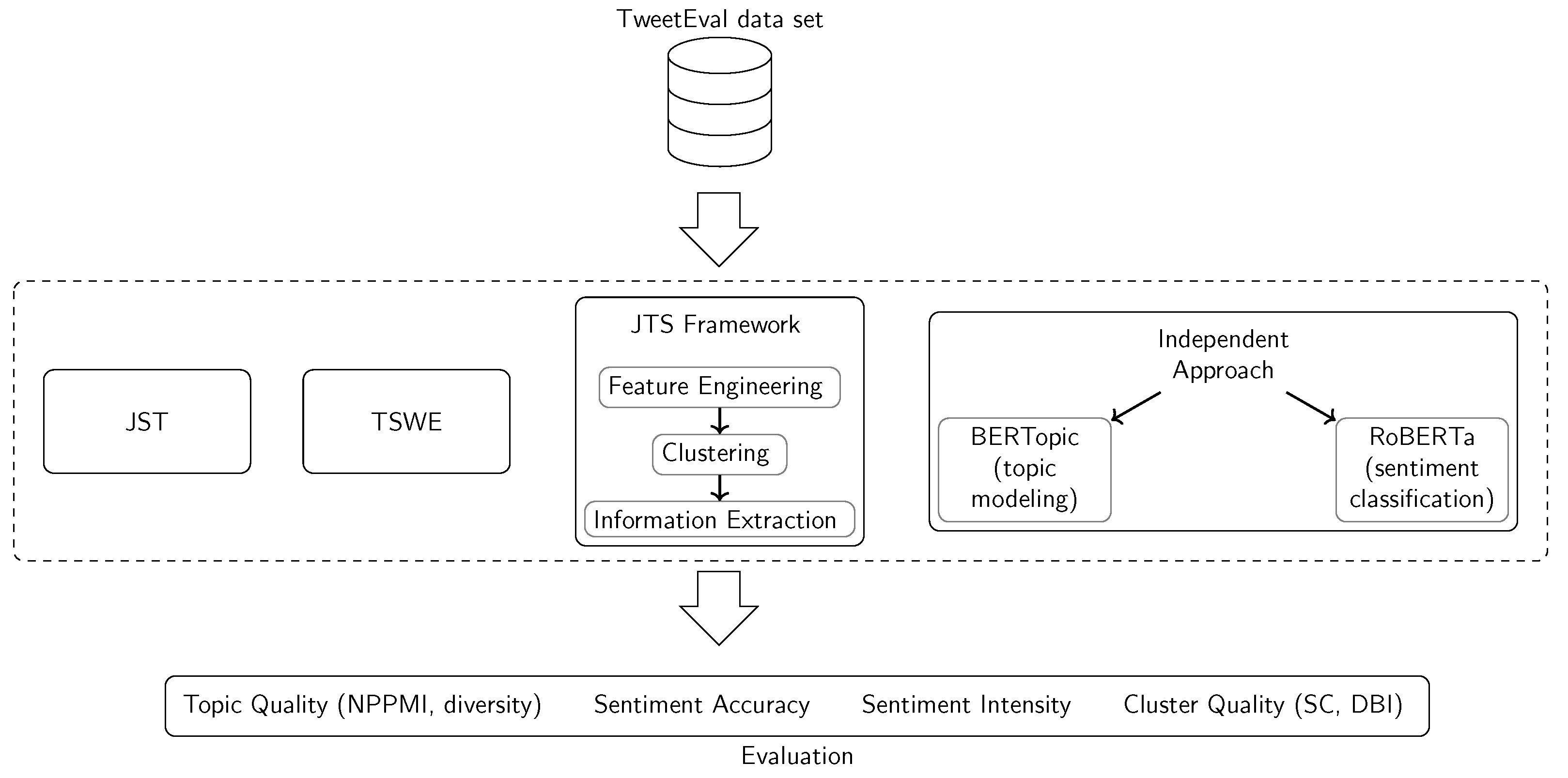
The following section explains the main methodology we developed for this study along with the experimental setup and the evaluation metrics. It starts with a detailed description of the presented approach and its implementation. Subsequently, the experimental setup based on the TweetEval test data set [43] is described. Figure 1 shows the overall design of this study including the evaluation where the proposed method is compared against similar approaches.
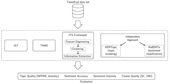
Figure 1.
Study design considered for the development and evaluation of the proposed topic-sentiment modeling framework.
3.1. JTS Framework
The presented JTS framework extracts topics associated with sentiments using a novel approach that clusters joint feature vectors that represent each social media post both semantically and with respect to the sentiment distribution. Subsequently, semantic and sentiment information are extracted from each cluster. The methodology therefore consists of a three-step procedure (excluding pre-processing) that is outlined in detail below. For clustering, we compared multiple methods in our experiments. The feature engineering process also entails dimensionality reduction, for which we investigated PCA and UMAP. Figure 2 depicts a visual overview of the JTS framework. Further along in this paper, we assumed that the model input is a collection of short-form textual social media posts .
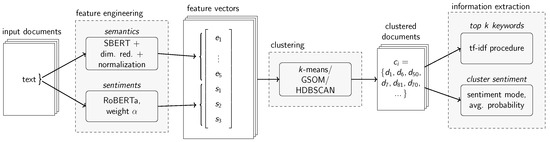
Figure 2.
Visual overview of the JTS framework.
3.1.1. Pre-Processing
The pre-processing of texts for the JTS model variants involves a two-fold approach. Only minimal pre-processing is required for the BERT-based language models used for sentiment analysis and embedding creation. They can handle language mostly as-is depending on the vocabulary of the underlying tokenizer, e.g., WordPiece for BERT [55]. For the keyword extraction process, the texts are pre-processed more extensively to prevent the occurrence of non-character tokens and redundancies in the output. Each text is therefore input to two independent pipelines resulting in two variants.
- Variant 1 (s. Section 3.1.2): User references and links are replaced with standardized tokens (“@user” and “http”) as they convey no relevant semantic information. Pota et al. [56] found that this can also be beneficial for sentiment classification. Moreover, excessive whitespace is stripped as it is not considered during tokenization. Due to the limited previous research conducted regarding text pre-processing for BERT-based language models, no additional steps are taken. Ek et al. [57] showed that BERT is generally quite robust to different punctuation. Furthermore, the inclusion of emojis can also improve sentiment classification results [58].
- Variant 2: (s. Section 3.1.4): Each text is pre-processed using a pipeline of (1) lowercasing, (2) removing special characters, non-character tokens and links, (3) removing user references and (4) converting tags to standalone words.
3.1.2. Feature Engineering
To cluster the input documents, a feature vector is obtained for each input text such that it is represented in a continuous joint topic-sentiment space. It captures both semantics and sentiments similar to the idea of a semantic space as proposed by Deerwester et al. [28] or Angelov [20]. Documents that are similar both semantically and concerning the associated sentiments are close in the joint topic-sentiment space and documents that are different are further apart. Effectively, each feature vector consists of a semantic part and a sentiment part which are concatenated to form a joint topic-sentiment representation.
The semantic part of the feature vector is obtained by computing a high-dimensional vector representation of each input text using SBERT [59]. This is possible due to the short length of social media posts which are usually within the token limit of BERT models. SBERT has furthermore been found to perform better on Semantic Textual Similarity (STS) tasks when compared to other approaches such as the Universal Sentence Encoder (USE) [60] and is also more computationally efficient [59]. The high-dimensional embedding vector is then reduced to a lower-dimensional representation with the help of dimensionality reduction. The dimensionality reduction techniques we considered for this study are UMAP and PCA. While PCA assumes that the data points lie in a linear subspace, UMAP involves manifold learning [61], making it a technique for non-linear dimensionality reduction. As Angelov [20] and Grootendorst [21] demonstrated, five-dimensional semantic vectors work well for topic modeling purposes which also turned out to be suitable for JTS framework after experimentation with different configurations.
For the sentiment part of the feature vector, the JTS framework follows a multi-class sentiment classification approach yielding “negative”, “neutral” or “positive” as output labels. Additionally, the classifier provides softmax probabilities for each of the three classes. The three sentiment probabilities are taken as a continuous representation of the sentiment distribution underlying each post. The sentiment classification models considered for the implementation were Twitter-RoBERTa-base-sentiment by Loureiro et al. [44] for English-only texts and Twitter-XLM-RoBERTa-base-sentiment by Barbieri et al. [42] for multilingual texts. Both were chosen due to their high empirical performance.
The entries of the semantic embedding vectors of the input texts, both in high- as well as low-dimensional form, do not have a fixed range of values. As this can skew the importance of semantics over sentiments in the final feature vector, the reduced semantic vector is scaled to unit length by dividing it by its norm [62]. This way, each entry can have an absolute value of one at maximum.
Finally, the normalized reduced embedding vector and the sentiment probabilities of each post are concatenated to achieve a continuous representation in a joint topic-sentiment space. To give the user some control over the importance of sentiments over semantics or vice versa, the sentiment part of the vector is weighted with a scalar weight value . A higher sentiment weight emphasizes sentiment differences more while a smaller value decreases the importance of sentiments.
3.1.3. Clustering
After generating joint topic-sentiment vectors for all posts to be analyzed, they are clustered to discover coherent collections of posts that are similar semantically and concerning the sentiment distribution. Since different clustering approaches come with different trade-offs, we considered three algorithms for the implementation: k-means, a GSOM, and HDBSCAN.
k-means: The classic k-means algorithm [63,64] is the simplest of all three clustering approaches. It requires the number of clusters k as a fixed input parameter and works well if the clusters are spherical. However, it might produce poor results when the clusters are non-spherical [65]. For our realization of the algorithm, we used a standard implementation using the k-means++ initialization method [66].
GSOM: Second, the GSOM by Alahakoon et al. [67] was considered as an unsupervised Artificial Neural Network (ANN) for clustering. It can be viewed as a dynamic version of the classic Self-Organizing Map (SOM) [68] that grows the neuron grid based on the input data. It is, therefore, not necessary to specify a static grid size, i.e., the number of clusters. After training the network, data points can be clustered by mapping each to its Best Matching Unit (BMU). For the implementation, we slightly modified the original GSOM algorithm to improve its handling of large amounts of input data. Specifically, the calculation of the growth threshold was modified to depend on three parameters: the spread factor , the number of input data points n, and some constant c. It can be written as . Furthermore, the weight initialization strategy was implemented as follows: Given the BMU, the location of the new neuron, and a third neighboring neuron, two cases are distinguished: (1) If the BMU has another neighboring neuron, the weight of the grown neuron is computed by evaluating Equation (1). (2) Else, the new neuron is grown in between the BMU and another neuron and the weight initialization follows Equation (2).
To prevent obscure initial weights beyond the value range of the training data, the weight vector of each new node was clipped component-wise if it exceeded a specified threshold for the minimum and maximum value. By default, the minimum threshold was set to and the maximum threshold to 1 based on the feature engineering output. The neighborhood radius and the learning rate were adapted based on the number of iterations and the network size to account for both factors. Specifically, the neighborhood radius was updated using the decaying formula in Equation (3) which incorporates the initial neighborhood radius , the current training iteration t and the total number of (training) iterations T. Moreover, the learning rate was adapted based on the number of nodes in the network using Equation (4) where are constants.
The respective default parameter values used in the experiments were , , .
HDBSCAN: HDBSCAN by [69] has become a popular density-based option for clustering, and has been used extensively in previous topic models such as top2vec and BERTopic [20,21]. It does not require a pre-determined number of clusters as input but might consider points as outliers that will not be assigned to a fixed cluster. Due to the hierarchical nature of the algorithm, it is possible to extract a cluster hierarchy from a run of HDBSCAN. For the experiments, we therefore extracted flat clustering results from the hierarchy to make the outputs comparable. The criterion used for obtaining the clusters was excess of mass which provides a global optimum to the problem of finding clusters with the highest stability [70].
3.1.4. Information Extraction
After the clustering step, the groups consist of numerical vectors that are associated with the respective input posts. To extract interpretable information about each cluster’s semantic topic and sentiment, the JTS framework leverages a slightly modified tf-idf procedure and cluster statistics.
Topic keywords. The top k keywords of each cluster are extracted based on word importance encoded in a tf-idf weight vector [71] for each cluster. The weight vector is computed in a two-step procedure:
- First, based on all input documents , the vocabulary and the respective idf values are learned.
- Subsequently, the documents within each cluster are concatenated to one string, and the tf-idf value is calculated using the term frequencies of the learned vocabulary words in the cluster and the previously learned idf values.
Formally, the tf-idf value for some term t in the vocabulary is calculated as in Equation (5) where c is a cluster of documents, the term frequency of term t in all documents of cluster c, n the total number of documents, and is the number of original documents containing t. Additionally, one is added to the inverse document frequency such that terms that occur in all documents are not completely ignored. It is also added to the numerator and denominator of the idf equation to prevent divisions by zero.
To reduce the occurrences of uninformative words in the final result, stopwords in the language(s) of the input documents are ignored when building the vocabulary for the tf-idf calculation. Very rare words that occur only in very few documents with document frequency and very frequent words with document frequency are ignored as well. The two thresholds and the stopwords are parameters of the keyword extraction algorithm. Finally, for each cluster c, the top k most important words (keywords) are extracted by computing its tf-idf vector and taking the k words with the highest respective values.
Cluster sentiment. To extract cluster sentiments, simple cluster statistics are used. The main cluster sentiments consist of the mode of the sentiment predictions within each cluster. As a supplementary measure of the sentiment intensity, the means of the corresponding sentiment probabilities are calculated. Analogously, the mean of the scores of each of the three sentiment classes can be calculated to obtain an average sentiment distribution for each cluster.
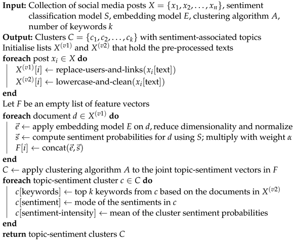
Algorithm 1 provides a more formal description of the entire JTS workflow. The procedures described in the above paragraphs are summarized in short functional descriptions within the larger algorithm.
| Algorithm 1: Pseudocode description of the JTS workflow |
 |
3.2. Experiments
Quantitatively, the JTS framework is comparable to existing joint topic-sentiment models. Therefore, it was benchmarked against the JST model by Lin and He [14] and TSWE by Fu et al. [15]. To also include a conceptually similar topic model based on a clustering-of-embedding-vectors approach, BERTopic [21] was combined with a transformer-based sentiment classification model [72] to compute both topics and sentiments. It can be viewed as a sequential-only approach that considers topics and sentiments independently.
3.2.1. Data and Setup
Given that joint topic-sentiment modeling fulfills two purposes simultaneously, topic extraction and sentiment classification, the data set used for quantitative assessment was the TweetEval test data set [43] for sentiment analysis taken from SemEval-2017, Task 4 [73]. It consists of 12,282 multi-thematic tweets in English and a true sentiment label corresponding to one of the three classes “negative“, “neutral”, and “positive”.
Each tweet was pre-processed as explained in Section 3.1. For JST and TSWE, the texts were additionally lemmatized, i.e., each word was transformed into its base form using wordnet [74], and English stopwords were removed. This decision was made based on the fact that both operate under the bag-of-words hypothesis.
All tested models were tuned to produce 60 topics in total, yielding a fine-grained overview of topics and their sentiments. As JST and TSWE produce topic-sentiment pairs where both the number of topics and sentiment components need to be specified, we parametrized the models with 3 sentiment components and 20 topic components per sentiment. Moreover, both models were injected with labeled sentiment paradigm words.
For the sequential BERTopic approach as well as the JTS framework, we used the Twitter-RoBERTa-base-sentiment model to compute sentiment predictions as it has been shown to outperform other state-of-the-art models for sentiment classification on English-language tweets [44]. Furthermore, BERTopic was parametrized to produce exactly 60 topics. We evaluated the JTS framework using different techniques for dimensionality reduction (PCA and UMAP) and clustering (k-means, a GSOM and HDBSCAN). All variants were adjusted to produce 60 clusters in total. To realize this for the GSOM, we stopped the network’s growth after 60 neurons had been reached. The sentiment weight during the generation of the feature vectors was always set to to emphasize semantics slightly higher. For the computation of semantic embedding vectors, we used the all-MiniLM-L12-v2 SBERT model for the English language. Finally, for all models, only words with an absolute document frequency and relative document frequency were considered in the keyword extraction process and English stopwords were ignored.
3.2.2. Software
All variants of the JTS framework were implemented in Python 3.9 [75] using NumPy 1.24.3 [76], scikit-learn 1.2.2 [77], SBERT as available in sentence-transformers 2.2.2 [59] and the transformers package version 4.29.2 [78]. We chose these packages due to their extensive functionality and ease of use. The unified Application Programming Interface (API) of the transformers package by Wolf et al. [78] also allows for the integration of current and future language models with even better performance or multilingual capabilities. The code for the full workflow is available by request. JST and TSWE were realized using the jointtsmodel package [79] version 1.6 as it provides a uniform, comparable implementation of these approaches. For BERTopic, we used the original implementation of Grootendorst [21] with version number 0.15.0.
3.2.3. Evaluation Metrics
The evaluation of the JTS framework mainly focused on semantic topic quality, sentiment prediction quality, and the uniformity of sentiments in each cluster.
Topic Quality. A major part of the quantitative evaluation is concerned with semantic cluster quality assessment which is equivalent to measuring topic quality and coherence in topic modeling. In the early days of topic modeling, perplexity (e.g., [17]) was often used as an evaluation metric for topic coherence. However, it has been shown to negatively correlate with human judgment, making it unsuited for what is supposed to be measured [80]. More recently, topic models have mostly been evaluated using information theoretic measures of topic coherence—in particular, the NPMI. It is based on the Positive Mutual Information (PMI) by Fano [81] and compares the probability of two words occurring together with the expected probability of them occurring together if independence is assumed. Equation (6) depicts its formal computation given a target word w and a context word c [82].
Bouma [83] normalized the equation with the self-information resulting in a value range of where a value of means that w and c never occur together, 0 that the words occur together as expected by random chance and 1 means that there is complete co-occurrence. Jurafsky and Martin [84] argued, however, that negative PMI values tend to be unreliable. If two words occur with individual probability , one would need to show that the probability of them occurring together is ≪ to state that they occur together less often than by chance. This assertion is hard to make unless the corpus of documents is huge. Moreover, it is unclear whether it is even possible to evaluate scores of unrelatedness with human judgment [82,84,85,86]. For this reason, the Positive Pointwise Mutual Information (PPMI) is often used instead [82,84] which is written as . It can also be normalized using the self-information yielding the Normalized Positive Pointwise Mutual Information (NPPMI) which takes on values in the range of where 1 means complete co-occurrence and 0 no significant co-occurrence. The formula is depicted in Equation (7).
For this paper’s experiments, we computed a topic coherence score for each cluster by taking the average NPPMI of the top k words of the respective topic-sentiment cluster. Subsequently, we calculated a model-level Topic Coherence (TC) score as the mean of all cluster-wise topic coherence scores [87].
As an additional measure for topic quality, we used the TD [37]. It provides a metric on how different the computed topics are with respect to their vocabulary and is defined as the fraction of unique words in the top k words of all topics. A topic diversity score close to 0 indicates that topics are likely redundant while a score close to 1 indicates that the topics are more varied. Moreover, as an overall measure of the Topic Quality (TQ) of a model, we used the product of the model-level topic coherence and topic diversity which can be written as as proposed by Dieng et al. [37].
Sentiment Quality. We measured the uniformity of the sentiments within a cluster using the fraction of sentiment labels that aligned with the global cluster sentiment label. It is referred to as the Sentiment Uniformity (SU) going further. The model-level sentiment uniformity was determined by calculating the mean of all cluster-wise values. Since each topic-sentiment model also computed sentiment labels for each input text, we measured the overall correctness of the predicted sentiments using the exact match ratio [88] which is referred to as Sentiment Exact Match Ratio (S-EMR) in the results section. It reflects the classification accuracy regarding the true sentiment labels and is calculated as the fraction of samples that were labeled correctly.
Cluster Quality. Since the JTS framework is a clustering-based approach, we also evaluated the quality of the clusters in the joint feature vector space. To realize this, we used two common measures for cluster quality: the Silhouette Coefficient (SC) [89] and the Davies–Bouldin Index (DBI) [90]. The SC is calculated for each sample based on cluster cohesion (mean intra-cluster distance) and separation (mean distance to all data points in the nearest neighboring cluster) as the difference of the two values divided by the maximum. An overall SC is then obtained by calculating the mean of all sample-wise scores. It has a range of where a value of 1 indicates that the clusters are internally cohesive and well-separated. The DBI, on the other hand, is computed as the average similarity of each cluster with its most similar cluster. Similarity, in this context, is the ratio between inter-cluster and intra-cluster distances. Lower DBI values indicate better clustering results, i.e., increased separation in between clusters and decreased variation within clusters. In our experiments, we calculated the average SC and DBI for all JTS variants. The output values cannot be compared to the adversarial approaches, however. JST and TSWE do not directly yield clusters of vectors due to their working principles. They are rather based on a generative process where words in documents are drawn from a distribution based on topics and sentiments. BERTopic furthermore operates on a purely semantic vector space that is different to the joint topic-sentiment space used by our JTS framework. A comparison of SC and DBI values would therefore be misleading.
4. Results
To maintain structure, the experimental results are divided into two parts: First, JST, TSWE, and BERTopic are compared against the JTS framework when PCA was used for dimensionality reduction. Second, the same comparison is made when UMAP was used instead.
4.1. JTS with PCA
The results of the quantitative evaluation when PCA was used for reducing the semantic embedding vectors to five dimensions are depicted in Table 4. The JTS approach consistently yielded better topic coherence than JST, TSWE and BERTopic for all three tested clustering algorithms. However, k-means and the GSOM performed poorly with respect to topic diversity and yielded overall topic quality scores similar to the other methods. An exception in this regard was the JTS approach using HDBSCAN which delivered the highest topic diversity. In terms of sentiment classification accuracy, JST and TSWE achieved a S-EMR of merely , making the classifications not particularly meaningful. The RoBERTa-based sentiment classification model used in the BERTopic and JTS approaches, in contrast, delivered a S-EMR of . While the sentiment uniformity was for JST and TSWE by definition of their working principles, the clusters produced by BERTopic and JTS with k-means and the GSOM were not as uniform. The interpretability of the respective cluster sentiments was therefore strongly limited. The value was better when HDBSCAN was used for clustering, delivering a sentiment uniformity of .
Table 4.
Performance metrics for 60 clusters computed on the TweetEval data set averaged over a total of 10 runs when PCA was used for dimensionality reduction for the JTS variants. The sentiment statistics marked with * were computed independently from the topic model and k denotes the number of keywords used for the computation of TC and TD. The best scores for each metric are highlighted in bold.
Cluster quality based on the SC was better for the JTS variants that used k-means and the GSOM for clustering. The SC score of still indicates that the clusters overlapped, though. HDBSCAN yielded a significantly worse SC of . The cause of this might be the “cluster” of outliers HDBSCAN produces. The DBI provides a slightly different picture with HDBSCAN achieving the lowest (best) score of . k-means and the GSOM were not far off, achieving marginally higher values of and .
Overall, the JTS framework using k-means and a GSOM performed similarly to the other approaches in combination with PCA for dimensionality reduction. It provided better sentiment classification accuracy and topic coherence for the cost of sentiment uniformity and topic diversity. When HDBSCAN was used for clustering, an improvement could also be achieved for topic diversity and the sentiment uniformity was high as well. However, the SC was significantly lower than for the variants based on k-means and the GSOM.
4.2. JTS with UMAP
The results were consistently better when UMAP was used for dimensionality reduction of the semantic embedding vectors. The output metrics are depicted in Table 5. All JTS variants vastly outperformed the other approaches in almost all aspects. Topic coherence was significantly higher across the board. Topic diversity was once again higher when HDBSCAN was used for clustering, although, k-means and the GSOM now yielded similar scores to JST, TSWE and BERTopic. Consequently, the overall topic quality scores were also higher for all JTS variants. In addition, the sentiment classification accuracy was again significantly better for all models that used the RoBERTa-based sentiment classification model. In contrast to the previous PCA-based variants, the JTS variants that used UMAP for dimensionality reduction also achieved high sentiment uniformity scores.
Table 5.
Performance metrics for 60 clusters computed on the TweetEval data set averaged over a total of 10 runs when UMAP was used for dimensionality reduction for the JTS variants. The sentiment statistics marked with * were computed independently from the topic model and k denotes the number of keywords used for the computation of TC and TD. The best scores for each metric are highlighted in bold.
The SC scores for all UMAP-based variants were noticeably higher compared to the JTS variants using PCA. k-means performed best, achieving a SC of , and the GSOM yielded a similar value of . HDBSCAN yielded a very low SC score of similarly to the previous section. Regarding the DBI, k-means and the GSOM both delivered a value of when combined with UMAP and HDBSCAN produced a slightly higher score of .
The results support the use of UMAP for a real-world JTS model. The clustering algorithms performed quite similarly overall, with the only exception being that HDBSCAN delivered better topic diversity but lower sentiment uniformity and worse SC and DBI scores. Compared to the other approaches, the JTS framework produced clusters of higher semantic quality and with better sentiment classification accuracy.
5. Discussion
The discussion is divided into a discussion of the experimental results and a discussion of the methodology.
5.1. Discussion of Results
The experiments show that the JTS framework can be a powerful tool for joint topic-sentiment modeling. It produced clusters that were of higher quality semantically when compared to previous approaches and yielded more accurate sentiments. The outputs were significantly better when UMAP was used for dimensionality reduction instead of PCA which supports its use in other topic modeling approaches such as [20,21]. However, UMAP does not scale nearly as well as PCA in terms of runtime and memory requirements for large data sets [91] which is why both techniques were considered for the experiments. Therefore, if very large data sets are to be analyzed, the JTS framework using PCA and HDBSCAN might be suited best. For all other scenarios, one of the variants using UMAP is recommended given the significantly improved results. The evaluation metrics are not as clear regarding the choice of the clustering algorithm. HDBSCAN was slightly advantageous for the PCA-based configuration in terms of semantic topic quality, sentiment uniformity and the average DBI. For the UMAP-based configuration, no consistently best clustering approach could be identified.
5.2. Discussion of the Methodology
As the experimental results indicate, the choice of the individual components of the JTS framework is not trivial. The results of previous studies [44,59] clearly favor the use of BERT for semantic embedding computation and sentiment classification and UMAP had an advantage over PCA in the experiments. However, the choice of the clustering algorithm largely depends on the needs of the user. k-means allows for a hard clustering where each data point is assigned to exactly one cluster but requires previous knowledge in the form of the number of assumed clusters as input. HDBSCAN was slightly superior in the experiments but often produced a large cluster of outliers when applied to data sets beyond the evaluation data. Such a collection of outliers is not coherent and does not provide any usable information. Moreover, a presumed number of clusters is once again required as input to extract flat clusters from the cluster hierarchy. The GSOM clustering approach does not require such input and computes the number of clusters naturally based on the accumulated error of the SOM nodes. It also assigns each data point to exactly one cluster like k-means. However, the topic-sentiment clusters computed with the GSOM algorithm had a slightly worse topic quality when compared to HDBSCAN. Simultaneously, however, the sentiment uniformity was higher with the GSOM algorithm in combination with UMAP. The GSOM algorithm additionally allows for the visualization of the learned neuron grid using a U-matrix-style visualization [92].
Despite their empirical performance, the BERT-based models used for the JTS variants present a significant bottleneck in terms of runtime and memory requirements. Moreover, many aspects of BERT-based transformer models are still not fully understood [93]. During semantic embedding generation for this study, for instance, it could be observed that the introduction of emojis tends to move the sentence embedding vectors of SBERT further apart in semantic space. Due to the scope of this paper, this effect was not examined further. However, it highlights the need for additional endeavors focusing on explainability. In many contexts, language models are used as black boxes with little transparency on how individual decisions are made and what the hidden representations mean [93]. This is also the case for the JTS framework as implemented for this study.
Concerning future research, the incorporation of additional dimensions in the feature vectors such as geographic space, time or image data should be explored. Additionally, the JTS framework might benefit from the integration of generative LLMs such as the Generative Pre-trained Transformer (GPT) or Llama-2 [94,95,96,97] in several ways. The GPT family of models specifically has been shown to be a powerful tool for sentiment analysis [98,99], even outperforming BERT-based models in some parts. GPT and Llama-2 have also successfully been utilized for topic modeling in approaches such as TopicGPT [100] and PromptTopic [101] which achieved similar performance to BERTopic or even improved upon it. However, such LLM-based techniques usually do not provide numeric embedding vectors or sentiment probabilities which are required by the JTS framework. They can therefore not be integrated into our method without major adjustments. Moreover, generative language models can be used to generate meaningful topic labels based on the cluster keywords and the associated tweets. In experimental test runs, the topic labels produced by GPT3.5 and Llama-2 were semantically correct, short, and understandable. Stammbach et al. [102] also showed that LLMs can be a powerful tool for the automatic evaluation of topic models.
Yet, there are several risks associated with the use of such LLMs. As the underlying training data sets are often not public (e.g., [94,97]), there is an even higher risk for unknown biases [103] compared to more transparent models such as BERT. As Pham et al. [100] also pointed out, some of the test data sets used for evaluating zero-shot classification performance might even be included in the unknown training data, thus skewing the results. Compared to variants of SBERT and RoBERTa—which already require a fair amount of computational resources—GPT and Llama-2 are even more resource-hungry and need a Graphics Processing Unit (GPU) with significant memory to run efficiently [101]. However, smaller models such as Mistral-7B [104] are becoming increasingly competitive, paving the way for the efficient use of LLMs in the future. Consequently, the development of a prompt-based framework for joint topic-sentiment modeling and a comparison to our current method presents a promising opportunity for a follow-up study.
6. Conclusions
This study introduced a novel framework for joint topic-sentiment modeling called the JTS framework. It works by merging semantic embedding vectors and sentiment probabilities into joint feature vectors which are then clustered. For semantic embedding generation and sentiment classification, pre-trained BERT-based transformer models are leveraged. From each respective cluster, the top k keywords and sentiment information are subsequently extracted using a tf-idf procedure and simple statistics. The JTS framework was experimentally compared against JST, TSWE, and an independent BERTopic plus sentiment classification approach. For the implementation of the experiments, several configurations of the JTS framework were considered. PCA and UMAP were compared for dimensionality reduction during the feature vector generation and k-means, a GSOM and HDBSCAN were considered for clustering. Overall, the JTS variants produced clusters with higher semantic topic quality and more accurate sentiment predictions compared to previous approaches.
In combination with PCA, HDBSCAN was most promising for clustering. It yielded an overall TQ score of based on the top 10 cluster keywords while the best score among all other approaches was . The clusters were uniform concerning the sentiment with a SU value of when compared to the independent BERTopic-based approach which only achieved a score of . For the UMAP-based variants of the JTS framework, the results were noticeably better and all clustering algorithms outperformed the adversarial approaches. Combined with HDBSCAN, our framework achieved an overall TQ of based on the top 10 keywords while the best value among the adversarial approaches was . The sentiment uniformity was also high for all clustering techniques in combination with UMAP ranging from to . The S-EMR was for all JTS variants while JST and TSWE only reached a respective value of .
Within a larger research context, the presented JTS framework allows for simultaneous semantic and sentiment analysis of short-form documents. Latent semantic topics are discovered in the form of clusters of texts, and each cluster is associated with a sentiment. The cluster sentiment contextualizes the semantic topic which might be useful in various contexts. One such example would be disaster management [105] where Neppalli et al. [18] showed that the sentiments of social media posts were linked to the distance to natural disasters. Sentiment-associated semantic clusters could, therefore, be leveraged for more efficient filtering of disaster-related social media posts. It also eases the interpretation of the clusters due to the additional layer of information.
Author Contributions
Conceptualization, D.H. and B.R.; methodology, D.H. and B.R.; software, D.H.; evaluation, D.H.; formal analysis, D.H.; investigation, D.H.; resources, B.R.; data curation, D.H.; writing—original draft preparation, D.H.; writing—review and editing, D.H. and B.R.; visualization, D.H.; supervision, B.R.; project administration, B.R.; funding acquisition, B.R. All authors have read and agreed to the published version of the manuscript.
Funding
This research was funded by the Austrian Research Promotion Agency (FFG) through the project MUSIG (Grant Number 886355). This work has also received funding from the European Commission—European Union under HORIZON EUROPE (HORIZON Research and Innovation Actions) under grant agreement 101093003 (HORIZON-CL4-2022-DATA-01-01). Views and opinions expressed are however those of the author(s) only and do not necessarily reflect those of the European Union—European Commission. Neither the European Commission nor the European Union can be held responsible for them.
Institutional Review Board Statement
Not applicable.
Informed Consent Statement
Not applicable.
Data Availability Statement
The raw data supporting the conclusions of this article will be made available by the authors on request.
Acknowledgments
We would like to thank the anonymous reviewers for taking the time and effort to review our manuscript. We appreciate the valuable and critical comments which helped us improve the quality of our study.
Conflicts of Interest
The authors declare no conflicts of interest.
References
- Pang, B.; Lee, L. Opinion Mining and Sentiment Analysis. Found. Trends® Inf. Retr. 2008, 2, 1–135. [Google Scholar] [CrossRef]
- Al-Qablan, T.A.; Mohd Noor, M.H.; Al-Betar, M.A.; Khader, A.T. A Survey on Sentiment Analysis and Its Applications. Neural Comput. Appl. 2023, 35, 21567–21601. [Google Scholar] [CrossRef]
- Egger, R.; Yu, J. A Topic Modeling Comparison Between LDA, NMF, Top2Vec, and BERTopic to Demystify Twitter Posts. Front. Sociol. 2022, 7, 886498. [Google Scholar] [CrossRef] [PubMed]
- Vayansky, I.; Kumar, S.A.P. A Review of Topic Modeling Methods. Inf. Syst. 2020, 94, 101582. [Google Scholar] [CrossRef]
- Yue, L.; Chen, W.; Li, X.; Zuo, W.; Yin, M. A Survey of Sentiment Analysis in Social Media. Knowl. Inf. Syst. 2019, 60, 617–663. [Google Scholar] [CrossRef]
- Crooks, A.; Croitoru, A.; Stefanidis, A.; Radzikowski, J. #Earthquake: Twitter as a Distributed Sensor System. Trans. GIS 2013, 17, 124–147. [Google Scholar] [CrossRef]
- Resch, B.; Usländer, F.; Havas, C. Combining Machine-Learning Topic Models and Spatiotemporal Analysis of Social Media Data for Disaster Footprint and Damage Assessment. Cartogr. Geogr. Inf. Sci. 2018, 45, 362–376. [Google Scholar] [CrossRef]
- Hu, B.; Jamali, M.; Ester, M. Spatio-Temporal Topic Modeling in Mobile Social Media for Location Recommendation. In Proceedings of the 2013 IEEE 13th International Conference on Data Mining, Washington, DC, USA, 7–10 December 2013; pp. 1073–1078. [Google Scholar] [CrossRef]
- Lwin, K.K.; Zettsu, K.; Sugiura, K. Geovisualization and Correlation Analysis between Geotagged Twitter and JMA Rainfall Data: Case of Heavy Rain Disaster in Hiroshima. In Proceedings of the 2015 2nd IEEE International Conference on Spatial Data Mining and Geographical Knowledge Services (ICSDM), Fuzhou, China, 8–10 July 2015; pp. 71–76. [Google Scholar] [CrossRef]
- Havas, C.; Wendlinger, L.; Stier, J.; Julka, S.; Krieger, V.; Ferner, C.; Petutschnig, A.; Granitzer, M.; Wegenkittl, S.; Resch, B. Spatio-Temporal Machine Learning Analysis of Social Media Data and Refugee Movement Statistics. ISPRS Int. J. Geo-Inf. 2021, 10, 498. [Google Scholar] [CrossRef]
- Havas, C.; Resch, B. Portability of Semantic and Spatial–Temporal Machine Learning Methods to Analyse Social Media for near-Real-Time Disaster Monitoring. Nat. Hazards 2021, 108, 2939–2969. [Google Scholar] [CrossRef]
- Stolerman, L.M.; Clemente, L.; Poirier, C.; Parag, K.V.; Majumder, A.; Masyn, S.; Resch, B.; Santillana, M. Using Digital Traces to Build Prospective and Real-Time County-Level Early Warning Systems to Anticipate COVID-19 Outbreaks in the United States. Sci. Adv. 2023, 9, eabq0199. [Google Scholar] [CrossRef]
- Wakamiya, S.; Kawai, Y.; Aramaki, E. Twitter-Based Influenza Detection After Flu Peak via Tweets with Indirect Information: Text Mining Study. JMIR Public Health Surveill. 2018, 4, e65. [Google Scholar] [CrossRef]
- Lin, C.; He, Y. Joint Sentiment/Topic Model for Sentiment Analysis. In Proceedings of the 18th ACM Conference on Information and Knowledge Management—CIKM’09, Hong Kong, China, 2–6 November 2009; pp. 375–384. [Google Scholar] [CrossRef]
- Fu, X.; Wu, H.; Cui, L. Topic Sentiment Joint Model with Word Embeddings. In Proceedings of the DMNLP@PKDD/ECML, Riva del Garda, Italy, 19–23 September 2016. [Google Scholar]
- Dermouche, M.; Kouas, L.; Velcin, J.; Loudcher, S. A Joint Model for Topic-Sentiment Modeling from Text. In Proceedings of the 30th Annual ACM Symposium on Applied Computing—SAC’15, New York, NY, USA, 13–17 April 2015; pp. 819–824. [Google Scholar] [CrossRef]
- Blei, D.M.; Ng, A.Y.; Jordan, M.I. Latent Dirichlet Allocation. J. Mach. Learn. Res. 2003, 3, 993–1022. [Google Scholar]
- Neppalli, V.K.; Caragea, C.; Squicciarini, A.; Tapia, A.; Stehle, S. Sentiment Analysis during Hurricane Sandy in Emergency Response. Int. J. Disaster Risk Reduct. 2017, 21, 213–222. [Google Scholar] [CrossRef]
- Sia, S.; Dalmia, A.; Mielke, S.J. Tired of Topic Models? Clusters of Pretrained Word Embeddings Make for Fast and Good Topics Too! In Proceedings of the 2020 Conference on Empirical Methods in Natural Language Processing (EMNLP), Online, 16–20 November 2020; pp. 1728–1736. [Google Scholar] [CrossRef]
- Angelov, D. Top2Vec: Distributed Representations of Topics. arXiv 2020, arXiv:2008.09470. [Google Scholar]
- Grootendorst, M. BERTopic: Neural Topic Modeling with a Class-Based TF-IDF Procedure. arXiv 2022, arXiv:2203.05794. [Google Scholar]
- Hoyle, A.; Sarkar, R.; Goel, P.; Resnik, P. Are Neural Topic Models Broken? In Proceedings of the Findings of the Association for Computational Linguistics: EMNLP 2022, Abu Dhabi, United Arab Emirates, 7–11 December 2022; pp. 5321–5344. [Google Scholar]
- Yau, C.K.; Porter, A.; Newman, N.; Suominen, A. Clustering Scientific Documents with Topic Modeling. Scientometrics 2014, 100, 767–786. [Google Scholar] [CrossRef]
- Suominen, A.; Toivanen, H. Map of Science with Topic Modeling: Comparison of Unsupervised Learning and Human-Assigned Subject Classification. J. Assoc. Inf. Sci. Technol. 2016, 67, 2464–2476. [Google Scholar] [CrossRef]
- Carron-Arthur, B.; Reynolds, J.; Bennett, K.; Bennett, A.; Griffiths, K.M. What is All the Talk about? Topic Modelling in a Mental Health Internet Support Group. BMC Psychiatry 2016, 16, 367. [Google Scholar] [CrossRef] [PubMed]
- Carter, D.J.; Brown, J.J.; Rahmani, A. Reading the High Court at A Distance: Topic Modelling The Legal Subject Matter and Judicial Activity of the High Court of Australia, 1903–2015. LawArXiv 2018. [Google Scholar] [CrossRef]
- Blauberger, M.; Heindlmaier, A.; Hofmarcher, P.; Assmus, J.; Mitter, B. The Differentiated Politicization of Free Movement of People in the EU. A Topic Model Analysis of Press Coverage in Austria, Germany, Poland and the UK. J. Eur. Public Policy 2023, 30, 291–314. [Google Scholar] [CrossRef]
- Deerwester, S.; Dumais, S.T.; Furnas, G.W.; Landauer, T.K.; Harshman, R. Indexing by Latent Semantic Analysis. J. Am. Soc. Inf. Sci. 1990, 41, 391–407. [Google Scholar] [CrossRef]
- Hofmann, T. Probabilistic Latent Semantic Analysis. In Proceedings of the Fifteenth Conference on Uncertainty in Artificial Intelligence—UAI’99, San Francisco, CA, USA, 30 July–1 August 1999; pp. 289–296. [Google Scholar]
- Choo, J.; Lee, C.; Reddy, C.K.; Park, H. UTOPIAN: User-Driven Topic Modeling Based on Interactive Nonnegative Matrix Factorization. IEEE Trans. Vis. Comput. Graph. 2013, 19, 1992–2001. [Google Scholar] [CrossRef] [PubMed]
- Griffiths, T.L.; Steyvers, M. Finding Scientific Topics. Proc. Natl. Acad. Sci. USA 2004, 101, 5228–5235. [Google Scholar] [CrossRef] [PubMed]
- Kingma, D.P.; Ba, J. Adam: A Method for Stochastic Optimization. arXiv 2017, arXiv:1412.6980. [Google Scholar] [CrossRef]
- Zhao, W.X.; Jiang, J.; Weng, J.; He, J.; Lim, E.P.; Yan, H.; Li, X. Comparing Twitter and Traditional Media Using Topic Models. In Advances in Information Retrieval; Clough, P., Foley, C., Gurrin, C., Jones, G.J.F., Kraaij, W., Lee, H., Mudoch, V., Eds.; Lecture Notes in Computer Science; Springer: Berlin/Heidelberg, Germany, 2011; pp. 338–349. [Google Scholar] [CrossRef]
- Dieng, A.B.; Ruiz, F.J.R.; Blei, D.M. The Dynamic Embedded Topic Model. arXiv 2019, arXiv:1907.05545. [Google Scholar] [CrossRef]
- Mikolov, T.; Chen, K.; Corrado, G.; Dean, J. Efficient Estimation of Word Representations in Vector Space. arXiv 2013, arXiv:1301.3781. [Google Scholar] [CrossRef]
- Le, Q.; Mikolov, T. Distributed Representations of Sentences and Documents. In Proceedings of the 31st International Conference on Machine Learning—PMLR, Beijing, China, 22–24 June 2014; pp. 1188–1196. [Google Scholar]
- Dieng, A.B.; Ruiz, F.J.R.; Blei, D.M. Topic Modeling in Embedding Spaces. Trans. Assoc. Comput. Linguist. 2020, 8, 439–453. [Google Scholar] [CrossRef]
- Lang, K. NewsWeeder: Learning to Filter Netnews. In Machine Learning Proceedings 1995; Prieditis, A., Russell, S., Eds.; Morgan Kaufmann: San Francisco, CA, USA, 1995; pp. 331–339. [Google Scholar] [CrossRef]
- Greene, D.; Cunningham, P. Practical Solutions to the Problem of Diagonal Dominance in Kernel Document Clustering. In Proceedings of the 23rd International Conference on Machine Learning (ICML’06), Pittsburgh, PA, USA, 25–29 June 2006; ACM Press: New York, NY, USA, 2006; pp. 377–384. [Google Scholar]
- Alharbi, A.S.M.; de Doncker, E. Twitter Sentiment Analysis with a Deep Neural Network: An Enhanced Approach Using User Behavioral Information. Cogn. Syst. Res. 2019, 54, 50–61. [Google Scholar] [CrossRef]
- Wei, J.; Liao, J.; Yang, Z.; Wang, S.; Zhao, Q. BiLSTM with Multi-Polarity Orthogonal Attention for Implicit Sentiment Analysis. Neurocomputing 2020, 383, 165–173. [Google Scholar] [CrossRef]
- Barbieri, F.; Espinosa Anke, L.; Camacho-Collados, J. XLM-T: Multilingual Language Models in Twitter for Sentiment Analysis and Beyond. In Proceedings of the Thirteenth Language Resources and Evaluation Conference, Marseille, France, 20–25 June 2022; pp. 258–266. [Google Scholar]
- Barbieri, F.; Camacho-Collados, J.; Espinosa Anke, L.; Neves, L. TweetEval: Unified Benchmark and Comparative Evaluation for Tweet Classification. In Proceedings of the Findings of the Association for Computational Linguistics: EMNLP 2020, Online, 16–20 November 2020; pp. 1644–1650. [Google Scholar] [CrossRef]
- Loureiro, D.; Barbieri, F.; Neves, L.; Espinosa Anke, L.; Camacho-collados, J. TimeLMs: Diachronic Language Models from Twitter. In Proceedings of the 60th Annual Meeting of the Association for Computational Linguistics: System Demonstrations, Dublin, Ireland, 22–27 May 2022; pp. 251–260. [Google Scholar] [CrossRef]
- Liu, Y.; Ott, M.; Goyal, N.; Du, J.; Joshi, M.; Chen, D.; Levy, O.; Lewis, M.; Zettlemoyer, L.; Stoyanov, V. RoBERTa: A Robustly Optimized BERT Pretraining Approach. arXiv 2019, arXiv:1907.11692. [Google Scholar]
- Conneau, A.; Khandelwal, K.; Goyal, N.; Chaudhary, V.; Wenzek, G.; Guzmán, F.; Grave, E.; Ott, M.; Zettlemoyer, L.; Stoyanov, V. Unsupervised Cross-lingual Representation Learning at Scale. In Proceedings of the 58th Annual Meeting of the Association for Computational Linguistics, Online, 5–10 July 2020; Jurafsky, D., Chai, J., Schluter, N., Tetreault, J., Eds.; Association for Computational Linguistics: Seattle, WA, USA, 2020; pp. 8440–8451. [Google Scholar] [CrossRef]
- Bojanowski, P.; Grave, E.; Joulin, A.; Mikolov, T. Enriching Word Vectors with Subword Information. Trans. Assoc. Comput. Linguist. 2017, 5, 135–146. [Google Scholar] [CrossRef]
- Camacho, K.; Portelli, R.; Shortridge, A.; Takahashi, B. Sentiment Mapping: Point Pattern Analysis of Sentiment Classified Twitter Data. Cartogr. Geogr. Inf. Sci. 2021, 48, 241–257. [Google Scholar] [CrossRef]
- Paul, D.; Li, F.; Teja, M.K.; Yu, X.; Frost, R. Compass: Spatio Temporal Sentiment Analysis of US Election What Twitter Says! In Proceedings of the 23rd ACM SIGKDD International Conference on Knowledge Discovery and Data Mining—KDD’17, Halifax, NS, Canada, 13–17 August 2017; pp. 1585–1594. [Google Scholar] [CrossRef]
- Kovacs-Györi, A.; Ristea, A.; Kolcsar, R.; Resch, B.; Crivellari, A.; Blaschke, T. Beyond Spatial Proximity—Classifying Parks and Their Visitors in London Based on Spatiotemporal and Sentiment Analysis of Twitter Data. ISPRS Int. J. Geo-Inf. 2018, 7, 378. [Google Scholar] [CrossRef]
- Lin, C.; He, Y.; Everson, R.; Ruger, S. Weakly Supervised Joint Sentiment-Topic Detection from Text. IEEE Trans. Knowl. Data Eng. 2012, 24, 1134–1145. [Google Scholar] [CrossRef]
- Liang, Q.; Ranganathan, S.; Wang, K.; Deng, X. JST-RR Model: Joint Modeling of Ratings and Reviews in Sentiment-Topic Prediction. Technometrics 2023, 65, 57–69. [Google Scholar] [CrossRef]
- Alaparthi, S.; Mishra, M. BERT: A Sentiment Analysis Odyssey. J. Mark. Anal. 2021, 9, 118–126. [Google Scholar] [CrossRef]
- Kotelnikova, A.; Paschenko, D.; Bochenina, K.; Kotelnikov, E. Lexicon-Based Methods vs. BERT for Text Sentiment Analysis. In Analysis of Images, Social Networks and Texts; Burnaev, E., Ignatov, D.I., Ivanov, S., Khachay, M., Koltsova, O., Kutuzov, A., Kuznetsov, S.O., Loukachevitch, N., Napoli, A., Panchenko, A., et al., Eds.; Lecture Notes in Computer Science; Springer: Cham, Switzerland, 2022; pp. 71–83. [Google Scholar] [CrossRef]
- Devlin, J.; Chang, M.W.; Lee, K.; Toutanova, K. BERT: Pre-training of Deep Bidirectional Transformers for Language Understanding. In Proceedings of the 2019 Conference of the North American Chapter of the Association for Computational Linguistics: Human Language Technologies, Volume 1 (Long and Short Papers), Minneapolis, MN, USA, 2–7 June 2019; pp. 4171–4186. [Google Scholar] [CrossRef]
- Pota, M.; Ventura, M.; Fujita, H.; Esposito, M. Multilingual Evaluation of Pre-Processing for BERT-based Sentiment Analysis of Tweets. Expert Syst. Appl. 2021, 181, 115119. [Google Scholar] [CrossRef]
- Ek, A.; Bernardy, J.P.; Chatzikyriakidis, S. How Does Punctuation Affect Neural Models in Natural Language Inference. In Proceedings of the Probability and Meaning Conference (PaM 2020), Gothenburg, Sweden, 3–5 June 2020; pp. 109–116. [Google Scholar]
- de Barros, T.M.; Pedrini, H.; Dias, Z. Leveraging Emoji to Improve Sentiment Classification of Tweets. In Proceedings of the 36th Annual ACM Symposium on Applied Computing—SAC ’21, Virtual, 22–26 March 2021; pp. 845–852. [Google Scholar] [CrossRef]
- Reimers, N.; Gurevych, I. Sentence-BERT: Sentence Embeddings Using Siamese BERT-Networks. In Proceedings of the 2019 Conference on Empirical Methods in Natural Language Processing and the 9th International Joint Conference on Natural Language Processing (EMNLP-IJCNLP), Hong Kong, China, 3–7 November 2019; pp. 3980–3990. [Google Scholar] [CrossRef]
- Cer, D.; Yang, Y.; Kong, S.Y.; Hua, N.; Limtiaco, N.; John, R.S.; Constant, N.; Guajardo-Cespedes, M.; Yuan, S.; Tar, C.; et al. Universal Sentence Encoder. arXiv 2018, arXiv:1803.11175. [Google Scholar] [CrossRef]
- Fefferman, C.; Mitter, S.; Narayanan, H. Testing the Manifold Hypothesis. J. Am. Math. Soc. 2016, 29, 983–1049. [Google Scholar] [CrossRef]
- Strang, G. Introduction to Linear Algebra, 5th ed.; Cambridge Press: Wellesley, MA, USA, 2016. [Google Scholar]
- Lloyd, S. Least Squares Quantization in PCM. IEEE Trans. Inf. Theory 1982, 28, 129–137. [Google Scholar] [CrossRef]
- MacQueen, J. Some Methods for Classification and Analysis of Multivariate Observations. In Proceedings of the Fifth Berkeley Symposium on Mathematical Statistics and Probability, Volume 1: Statistics; University of California Press: Berkeley, CA, USA, 1967; Volume 5.1, pp. 281–298. [Google Scholar]
- Jin, X.; Han, J. K-Means Clustering. In Encyclopedia of Machine Learning; Sammut, C., Webb, G.I., Eds.; Springer: Boston, MA, USA, 2010; pp. 563–564. [Google Scholar] [CrossRef]
- Arthur, D.; Vassilvitskii, S. K-Means++: The Advantages of Careful Seeding. In Proceedings of the Eighteenth Annual ACM-SIAM Symposium on Discrete Algorithms—SODA ’07, New Orleans, LA, USA, 7–9 January 2007; pp. 1027–1035. [Google Scholar]
- Alahakoon, D.; Halgamuge, S.; Srinivasan, B. Dynamic Self-Organizing Maps with Controlled Growth for Knowledge Discovery. IEEE Trans. Neural Netw. 2000, 11, 601–614. [Google Scholar] [CrossRef]
- Kohonen, T. The Hypermap Architecture. In Artificial Neural Networks; Kohonen, T., Mäkisara, K., Simula, O., Kangas, J., Eds.; North-Holland: Amsterdam, The Netherlands, 1991; pp. 1357–1360. [Google Scholar] [CrossRef]
- Campello, R.J.G.B.; Moulavi, D.; Sander, J. Density-Based Clustering Based on Hierarchical Density Estimates. In Advances in Knowledge Discovery and Data Mining; Pei, J., Tseng, V.S., Cao, L., Motoda, H., Xu, G., Eds.; Lecture Notes in Computer Science; Springer: Berlin/Heidelberg, Gernmay, 2013; pp. 160–172. [Google Scholar] [CrossRef]
- Malzer, C.; Baum, M. A Hybrid Approach To Hierarchical Density-based Cluster Selection. In Proceedings of the 2020 IEEE International Conference on Multisensor Fusion and Integration for Intelligent Systems (MFI), Virtual, 14–16 September 2020; pp. 223–228. [Google Scholar] [CrossRef]
- Salton, G. Automatic Text Processing: The Transformation, Analysis, and Retrieval of Information by Computer; Addison-Wesley Series in Computer Science; Addison-Wesley: Boston, MA, USA, 1989. [Google Scholar]
- Camacho-Collados, J.; Rezaee, K.; Riahi, T.; Ushio, A.; Loureiro, D.; Antypas, D.; Boisson, J.; Espinosa Anke, L.; Liu, F.; Martínez Cámara, E. TweetNLP: Cutting-Edge Natural Language Processing for Social Media. In Proceedings of the 2022 Conference on Empirical Methods in Natural Language Processing: System Demonstrations, Abu Dhabi, United Arab Emirates, 7–11 December 2022; pp. 38–49. [Google Scholar]
- Rosenthal, S.; Farra, N.; Nakov, P. SemEval-2017 Task 4: Sentiment Analysis in Twitter. In Proceedings of the 11th International Workshop on Semantic Evaluation (SemEval-2017), Vancouver, BC, Canada, 3–4 August 2017; pp. 502–518. [Google Scholar] [CrossRef]
- Fellbaum, C. (Ed.) WordNet: An Electronic Lexical Database; Language, Speech, and Communication; MIT Press: Cambridge, MA, USA, 1998. [Google Scholar]
- van Rossum, G. Python Tutorial [Technical Report]; CWI (National Research Institute for Mathematics and Computer Science): Amsterdam, The Netherlands, 1995. [Google Scholar]
- Harris, C.R.; Millman, K.J.; van der Walt, S.J.; Gommers, R.; Virtanen, P.; Cournapeau, D.; Wieser, E.; Taylor, J.; Berg, S.; Smith, N.J.; et al. Array Programming with NumPy. Nature 2020, 585, 357–362. [Google Scholar] [CrossRef]
- Pedregosa, F.; Varoquaux, G.; Gramfort, A.; Michel, V.; Thirion, B.; Grisel, O.; Blondel, M.; Prettenhofer, P.; Weiss, R.; Dubourg, V.; et al. Scikit-Learn: Machine Learning in Python. J. Mach. Learn. Res. 2011, 12, 2825–2830. [Google Scholar]
- Wolf, T.; Debut, L.; Sanh, V.; Chaumond, J.; Delangue, C.; Moi, A.; Cistac, P.; Rault, T.; Louf, R.; Funtowicz, M.; et al. Transformers: State-of-the-Art Natural Language Processing. In Proceedings of the 2020 Conference on Empirical Methods in Natural Language Processing: System Demonstrations, Online, 16–20 November 2020; Liu, Q., Schlangen, D., Eds.; Association for Computational Linguistics: Seattle, WA, USA, 2020; pp. 38–45. [Google Scholar] [CrossRef]
- victor7246. Victor7246/Jointtsmodel. Available online: https://github.com/victor7246/jointtsmodel (accessed on 7 March 2024).
- Chang, J.; Gerrish, S.; Wang, C.; Boyd-graber, J.; Blei, D. Reading Tea Leaves: How Humans Interpret Topic Models. In Advances in Neural Information Processing Systems; Curran Associates, Inc.: Red Hook, NY, USA, 2009; Volume 22. [Google Scholar]
- Fano, R.M. Transmission of Information: A Statistical Theory of Communications, 3rd ed.; MIT Press: Cambridge, MA, USA, 1966. [Google Scholar]
- Church, K.W.; Hanks, P. Word Association Norms, Mutual Information, and Lexicography. In Proceedings of the 27th Annual Meeting of the Association for Computational Linguistics, Vancouver, BC, Canada, 26–29 June 1989; pp. 76–83. [Google Scholar] [CrossRef]
- Bouma, G. Normalized (Pointwise) Mutual Information in Collocation Extraction. Proc. GSCL 2009, 30, 31–40. [Google Scholar]
- Jurafsky, D.; Martin, J.H. Speech and Language Processing, 3rd ed. Draft. Available online: https://web.stanford.edu/~jurafsky/slp3/ (accessed on 23 May 2023).
- Niwa, Y.; Nitta, Y. Co-Occurrence Vectors from Corpora vs. Distance Vectors from Dictionaries. In Proceedings of the COLING 1994 Volume 1: The 15th International Conference on Computational Linguistics, Kyoto, Japan, 5–9 August 1994. [Google Scholar]
- Dagan, I.; Marcus, S.; Markovitch, S. Contextual Word Similarity and Estimation from Sparse Data. In Proceedings of the 31st Annual Meeting on Association for Computational Linguistics—ACL ’93, Columbus, OH, USA, 22–26 June 1993; pp. 164–171. [Google Scholar] [CrossRef]
- Terragni, S.; Fersini, E.; Galuzzi, B.G.; Tropeano, P.; Candelieri, A. OCTIS: Comparing and Optimizing Topic Models Is Simple! In Proceedings of the 16th Conference of the European Chapter of the Association for Computational Linguistics: System Demonstrations, Online, 19–23 April 2021; pp. 263–270. [Google Scholar] [CrossRef]
- Sorower, M.S. A Literature Survey on Algorithms for Multi-Label Learning. Or. State Univ. Corvallis 2010, 18, 25. [Google Scholar]
- Rousseeuw, P.J. Silhouettes: A Graphical Aid to the Interpretation and Validation of Cluster Analysis. J. Comput. Appl. Math. 1987, 20, 53–65. [Google Scholar] [CrossRef]
- Davies, D.L.; Bouldin, D.W. A Cluster Separation Measure. IEEE Trans. Pattern Anal. Mach. Intell. 1979, PAMI-1, 224–227. [Google Scholar] [CrossRef]
- McInnes, L. UMAP Documentation: Release 0.5; UMAP: Odisha, India, 2023. [Google Scholar]
- Ultsch, A.; Siemon, H.P. Kohonen’s Self Organizing Feature Maps for Exploratory Data Analysis. In Proceedings of the International Neural Network Conference (INNC-90), Paris, France, 9–13 July 1990; Widrow, B., Angeniol, B., Eds.; Springer: Dordrecht, The Netherlands, 1990; Volume 1, pp. 305–308. [Google Scholar]
- Zini, J.E.; Awad, M. On the Explainability of Natural Language Processing Deep Models. ACM Comput. Surv. 2022, 55, 103:1–103:31. [Google Scholar] [CrossRef]
- OpenAI. GPT-4 Technical Report. arXiv 2023, arXiv:2303.08774. [Google Scholar] [CrossRef]
- Radford, A.; Narasimhan, K.; Salimans, T.; Sutskever, I. mproving Language Understanding by Generative Pre-Training [Technical Report]. OpenAI. 2018. Available online: https://cdn.openai.com/research-covers/language-unsupervised/language_understanding_paper.pdf (accessed on 15 July 2023).
- Brown, T.; Mann, B.; Ryder, N.; Subbiah, M.; Kaplan, J.D.; Dhariwal, P.; Neelakantan, A.; Shyam, P.; Sastry, G.; Askell, A.; et al. Language Models Are Few-Shot Learners. In Advances in Neural Information Processing Systems; Curran Associates, Inc.: Red Hook, NY, USA, 2020; Volume 33, pp. 1877–1901. [Google Scholar]
- Touvron, H.; Martin, L.; Stone, K.; Albert, P.; Almahairi, A.; Babaei, Y.; Bashlykov, N.; Batra, S.; Bhargava, P.; Bhosale, S.; et al. Llama 2: Open Foundation and Fine-Tuned Chat Models. arXiv 2023, arXiv:2307.09288. [Google Scholar] [CrossRef]
- Kheiri, K.; Karimi, H. SentimentGPT: Exploiting GPT for Advanced Sentiment Analysis and Its Departure from Current Machine Learning. arXiv 2023, arXiv:2307.10234. [Google Scholar] [CrossRef]
- Wang, Z.; Pang, Y.; Lin, Y. Large Language Models Are Zero-Shot Text Classifiers. arXiv 2023, arXiv:2312.01044. [Google Scholar] [CrossRef]
- Pham, C.M.; Hoyle, A.; Sun, S.; Iyyer, M. TopicGPT: A Prompt-based Topic Modeling Framework. arXiv 2023, arXiv:2311.01449. [Google Scholar] [CrossRef]
- Wang, H.; Prakash, N.; Hoang, N.K.; Hee, M.S.; Naseem, U.; Lee, R.K.W. Prompting Large Language Models for Topic Modeling. arXiv 2023, arXiv:2312.09693. [Google Scholar] [CrossRef]
- Stammbach, D.; Zouhar, V.; Hoyle, A.; Sachan, M.; Ash, E. Revisiting Automated Topic Model Evaluation with Large Language Models. In Proceedings of the 2023 Conference on Empirical Methods in Natural Language Processing, Singapore, 6–10 December 2023; Bouamor, H., Pino, J., Bali, K., Eds.; Association for Computational Linguistics: Seattle, WA, USA, 2023; pp. 9348–9357. [Google Scholar] [CrossRef]
- Weidinger, L.; Mellor, J.; Rauh, M.; Griffin, C.; Uesato, J.; Huang, P.S.; Cheng, M.; Glaese, M.; Balle, B.; Kasirzadeh, A.; et al. Ethical and Social Risks of Harm from Language Models. arXiv 2021, arXiv:2112.04359. [Google Scholar] [CrossRef]
- Jiang, A.Q.; Sablayrolles, A.; Mensch, A.; Bamford, C.; Chaplot, D.S.; de las Casas, D.; Bressand, F.; Lengyel, G.; Lample, G.; Saulnier, L.; et al. Mistral 7B. arXiv 2023, arXiv:2310.06825. [Google Scholar] [CrossRef]
- Ragini, J.R.; Anand, P.M.R.; Bhaskar, V. Big Data Analytics for Disaster Response and Recovery through Sentiment Analysis. Int. J. Inf. Manag. 2018, 42, 13–24. [Google Scholar] [CrossRef]

Disclaimer/Publisher’s Note: The statements, opinions and data contained in all publications are solely those of the individual author(s) and contributor(s) and not of MDPI and/or the editor(s). MDPI and/or the editor(s) disclaim responsibility for any injury to people or property resulting from any ideas, methods, instructions or products referred to in the content. |
© 2024 by the authors. Licensee MDPI, Basel, Switzerland. This article is an open access article distributed under the terms and conditions of the Creative Commons Attribution (CC BY) license (https://creativecommons.org/licenses/by/4.0/).