IUAutoTimeSVD++: A Hybrid Temporal Recommender System Integrating Item and User Features Using a Contractive Autoencoder ^†

Abstract

Collaborative filtering (CF), a fundamental technique in personalized Recommender Systems, operates by leveraging user–item preference interactions. Matrix factorization remains one of the most prevalent CF-based methods. However, recent advancements in deep learning have spurred the development of hybrid models, which extend matrix factorization, particularly with autoencoders, to capture nonlinear item relationships. Despite these advancements, many proposed models often neglect dynamic changes in the rating process and overlook user features. This paper introduces IUAutoTimeSVD++, a novel hybrid model that builds upon autoTimeSVD++. By incorporating item–user features into the timeSVD++ framework, the proposed model aims to address the static nature and sparsity issues inherent in existing models. Our model utilizes a contractive autoencoder (CAE) to enhance the capacity to capture a robust and stable representation of user-specific and item-specific features, accommodating temporal variations in user preferences and leveraging item characteristics. Experimental results on two public datasets demonstrate IUAutoTimeSVD++’s superiority over baseline models, affirming its effectiveness in capturing and utilizing user and item features for temporally adaptive recommendations.

1. Introduction

In the era of big data, Recommender Systems (RS) [1] have become crucial for personalized recommendations and an indispensable part of our daily life. These systems facilitate the user’s experience by helping them to make decisions based on their historical preferences, such as ratings, clicks, saved carts, wishlists, and order history. Collaborative filtering (CF) [2], which relies on user preferences, remains a highly successful recommendation approach. Among collaborative filtering methods, matrix factorization, a latent factor model, gained popularity after its success in the Netflix prize challenge [3]. It continues to yield competitive results when compared with state-of-the-art deep learning-based models, as proved recently in [4,5]. Matrix factorization approximates the rating matrix $\mathbf{R}$ using two lower-rank matrices, $\mathbf{P}$ and $\mathbf{Q}$, where k denotes the latent factor dimension. Despite the success of collaborative filtering, it struggles with sparsity (a lot of items without ratings) and cold-start (recommendations for a new user, for example) issues, particularly when recommending items to new users or handling new items. As the field of recommender systems advances, to address this limitation researchers have begun incorporating modern techniques such as deep learning (DL) [6,7] to propose innovative models. Other approaches adopt a hybrid strategy such as in [8,9,10], which combine latent factor models such as matrix factorization and deep learning techniques such as autoencoders or CNNs to leverage the benefits of both such as dimensionality reduction, efficient representation learning, and modeling of complex features. In this paper, our primary contribution lies in extending our previous model, autoTimeSVD++ [11], by incorporating user features. The proposed model integrates both user and item features, along with a temporal aspect based on timeSVD++ [12]. Our novel model, named IUAutoTimeSVD++, represents a temporal hybrid model that seamlessly integrates two techniques: temporal dynamics matrix factorization (timeSVD++) and the contractive autoencoder (CAE) [13]. Leveraging the effectiveness of CAE in feature extraction, it synergizes with temporal dynamics matrix factorization to enhance the model’s performance and recommendation accuracy. In light of this hybrid model, the present paper addresses the following research questions:

• How can integrate user–item features within the timeSVD++ model to enhance the accuracy of rating predictions?
• How to compare the performance of the IUAutoTimeSVD++ model with the baseline models, assessing its superiority and effectiveness?
• How can we quantify the impact and significance of each component in our model to understand their individual contributions to improving recommendation predictions?
• What are the limitations of the proposed model to provide insights into its potential areas for improvement?

By answering these research questions, our objective is to conduct a thorough evaluation of the IUAutoTimeSVD++ model, providing a detailed examination of its strengths, limitations, and possible future directions. The paper’s structure is organized as follows: The next section presents and discusses related works in the field of recommender systems by considering two main collaborative filtering methods: MF and PMF and its extensions. Section 3 is dedicated to presenting the architecture, prediction formula, and optimization process of the IUAutoTimeSVD++ model. In Section 4, we delve into the experimental results and present a comprehensive discussion of the findings. Finally, we summarize the main findings, underscore the contributions of our work in developing the IUAutoTimeSVD++ model, and suggest potential avenues for future research.

2. Related Work

In this section, our focus is on various collaborative filtering models, which include matrix factorization and its extensions, as well as contrastive learning (CL)-based models. The study is divided into three parts: the extensions of the native matrix factorization, probabilistic matrix factorization (PMF), and CL-based models as follows:

2.1. MF Extensions

Matrix factorization (MF) [14] has been a fundamental technique in recommendation systems, but researchers have continually sought to enhance its capabilities by suggesting novel extensions. Several models have been introduced to address specific challenges and incorporate additional data modalities, leading to improved recommendation accuracy and performance. One of the earliest extensions of MF is SVD++ [14] which incorporates the implicit feedback of users. Another extension of MF is timeSVD+ [12] which extends SVD++ by leveraging the time factor; this extension allows the model to extract user preferences over time. Another extension of MF is Visual Bayesian Personalized Ranking (VBPR) [15], which integrates visual information, such as images. By considering item visual features extracted using a CNN model, VBPR aims to make more informed and accurate recommendations, especially in the fashion domain, particularly when visual content plays a crucial role in item preferences. EMF (Explainable Matrix Factorization) [16] represents another notable extension of traditional matrix factorization techniques, aimed at achieving a balance between recommendation accuracy and interpretability. This model adopts a neighborhood explainability style to provide clear and intuitive explanations for its recommendations, making it more transparent and understandable to users. Another notable advancement is NeuMF (Neural Collaborative Filtering) [17]. It extends MF through a combination of two models: GMF, which is a generalized matrix factorization using pairwise product (Hadamard product), and an MLP-based model. Although NeuMF succeeds in capturing complex patterns, it suffers from computing efficiency issues due to the high cost of training the MLP branch of this model [4]. AutoSVD++ [8] introduces a hybrid approach by incorporating item features through a contractive autoencoder (CAE) into the SVD++ model. By leveraging item features, AutoSVD++ addresses the sparsity problem inherent in recommendation data, leading to improved recommendation accuracy and coverage. Similarly, SSAERec [10] extends the SVD++ [14] by adopting a hybrid strategy that involves utilizing a stacked autoencoder to extract item features. These extracted features are then incorporated into the latent factor model, which considers implicit feedback to enhance the recommendation process.

This review of related work is summarized in

Table 1. Matrix factorization extension models.

Baseline Model	Extension
MF [14]	Model	Type	Technique	Year	Time factor	User features	Item features	Visual features
	SVD++ [14]	Implicit feedback	Dot product	2008
	timeSVD++ [12]	Temporal	Dot product	2009	✔
	VBPR [15]	Visual	CNN	2016				✔
	EMF [16]	Explainability	Similarity	2016
	autoSVD++ [8]	Hybrid	Autoencoder	2017			✔
	NeuMF [17]	Embedding	MLP	2017
	SSAERec [10]	Hybrid	Autoencoder	2021			✔

:

2.2. PMF Extensions

In this context, probabilistic matrix factorization (PMF) [18] stands as a foundational model. PMF is a technique used in CF models for recommendation systems. The fundamental principle behind PMF is to represent the user–item interaction matrix as a probabilistic model. The model formalized both user and item latent factors as random variables following a Gaussian distribution (normal distribution) with a zero mean. ConvMF (convolutional matrix factorization) [9] serves as an extension, introducing a convolutional neural network (CNN) to seamlessly integrate textual item reviews with item embedding. Leveraging user reviews, ConvMF enhances traditional PMF to provide more personalized and context-aware recommendations. Another notable extension is DBPMF (deep probabilistic matrix factorization) [19], which applies a CNN to extract user–item features, and the results are then averaged with PMF.

A comprehensive summary of the studies on PMF extensions is presented in

Table 2. Probabilistic matrix factorization extension models.

Baseline Model	Extension
PMF [18]	Model	Type	Technique	Year	Time factor	User features	Item features	Visual features
	ConvMF [9]	Textual	CNN	2016			✔
	DBPMF [19]	Hybrid	CNN	2019		✔	✔

:

2.3. Contrastive Collaborative Filtering

Contrastive learning (CL) has emerged as a promising approach in recommendation systems, garnering significant attention in recent years. CL involves learning representations of users and items by contrasting positive interactions with negative interactions. This methodology aims to capture underlying patterns in user–item interactions, thereby enhancing recommendation quality. In CL-based recommendation, positive interactions, such as user–item interactions indicating preference or engagement, are treated as positive samples, while negative interactions, such as non-interactions or randomly sampled items, serve as negative samples. By training the recommendation model to maximize the similarity between positive user–item pairs and minimize the similarity between negative user–item pairs in the learned representation space, CL-based recommendation endeavors to learn more informative representations of users and items. This approach enables the model to capture nuanced preferences, thereby improving its ability to make accurate recommendations. Recent research efforts, such as [20], have integrated CL into collaborative filtering by extending graph neural networks (GNNs). These models leverage bipartite graph representations of user–item interactions and incorporate high-order interactions and message passing to learn augmented user and item representations. Additionally, other recent models, such as [21], further enhance GNN-based approaches by learning different intents. These advancements highlight the growing importance and potential of CL-based techniques in recommendation systems.

Despite the significant advancements in recommender system models—particularly, the hybridization of collaborative techniques with deep learning (DL) models such as convolutional neural networks (CNNs) and autoencoders for extracting item features and the advancements in integrating the contrastive learning (CL) in recommendation, which is a promising and ongoing research area—certain crucial aspects remain overlooked. Many existing models heavily rely on static approaches like matrix factorization (MF) or probabilistic matrix factorization (PMF), disregarding the dynamic nature of user preferences over time. User rating tastes evolve with time; for instance, preferences for movie genres may differ between weekdays and weekends. Additionally, user behavior may vary based on seasonal factors; for example, individuals might purchase warm clothing during the winter season and switch to beachwear during the summer. Furthermore, while some models focus solely on extracting item features, they often neglect the equally important user features. In light of these limitations, our motivation drives the proposition of the IUAutoTimeSVD++ model. By integrating both item and user features within a temporal dynamic framework, IUAutoTimeSVD++ aims to address sparsity issues, extract meaningful user–item features, and effectively capture changes in user preferences over time through the utilization of timeSVD++.

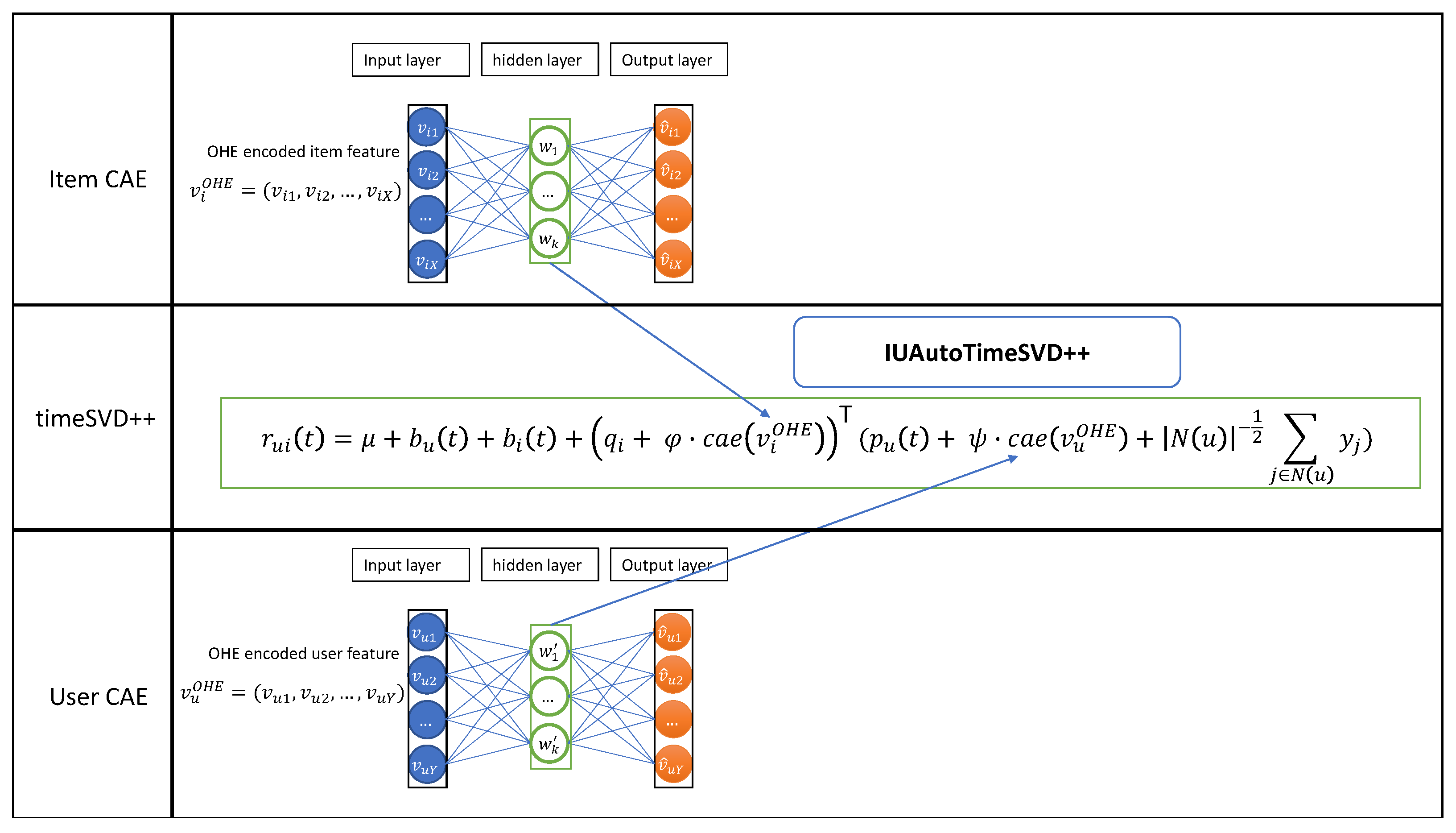
3. Our Model IUAutoTimeSVD++

3.1. Preliminary

Prior to delving into the exposition of the model architecture, we provide a comprehensive definition of the symbols employed in current article, as summarized in

Table 3. Notations and symbols used in the article.

Notation	Description
$\mathcal{U}$	The user’s set defined as $\{u_1,u_2,\dots ,u_m\}$
$\mathcal{I}$	The item’s set defined as $\{i_1,i_2,\dots ,i_n\}$
n	The number of items where $n\in \mathbb{N}$
m	The number of users where $m\in \mathbb{N}$
$v_i^{OHE}$	OHE item features vector $v_i^{OHE}=\{x_1,x_2,\dots ,x_X\}$ of size X
$v_u^{OHE}$	OHE user features vector $v_u^{OHE}=\{x_1,x_2,\dots ,x_Y\}$ of size Y
$\mathbf{R}$	Interaction of rating matrix
$\mathbf{Q}$	Low rank matrix representing items
$\mathbf{P}$	Low rank matrix representing users
K	The latent factors space
k	The latent factors dimension
$r_{ui}$	The rating value provided by a user u of an item i
$r_{ui\left(t\right)}$	The rating value at the time t
CAE	Contractive autoencoder
SVD	Single value decomposition
SGD	Stochastic gradient Descent

:

3.2. Model Architecture

The proposed IUAutoTimeSVD++ model extends the temporal latent factors of the timeSVD++ model by incorporating a comprehensive representation of user–item features, facilitated by the powerful contractive autoencoder (CAE). Leveraging the CAE as an efficient technique for extracting meaningful representations of both user and item features, our model aims to enhance the accuracy of recommendations.

The architecture of the IUAutoTimeSVD++ model comprises the following key components:

3.2.1. Temporal Latent Factors Model

The timeSVD++ [12] model, an extension of the conventional collaborative filtering model SVD++ (Singular Value Decomposition Plus Plus) [14], builds upon its foundations to incorporate temporal dynamics. This extension allows the model to adapt to changes in user preferences over time. TimeSVD++ introduces several modifications to the original SVD++ formulation, affecting components such as item bias, user bias, and the introduction of a new term: time deviation $de{v}_u^{OHE}\left(t\right)$ to account for temporal variability. Each component comprises two parts: an initial static part and a dynamic part to capture evolving user preferences. The timeSVD++ model contains the following components:

Item Bias

The item bias is split into two parts, the initial static $b_i$ and dynamic binning $Bin$, depending on the time as follows:

$$b_i\left(t\right)=b_i+b_{i,\mathrm{Bin}\left(t\right)}$$

(1)

Time Deviation

A deviation time to capture the rating time variability in linear form is as follows:

$${\mathrm{dev}}_u\left(t\right)=\mathrm{sign}(t-t_u)·{|t-t_u|}^{\beta }$$

(2)

User Bias

We update the user bias by introducing the time deviation $de{v}_u\left(t\right)$.

$$b_u\left(t\right)=b_u+{\alpha }_u·{\mathrm{dev}}_u\left(t\right)+b_{u,t}$$

(3)

User Latent Factors

In the same way as user bias, we introduce the deviation time in the user latent factors formula as follows:

$$p_u\left(t\right)=p_u+{\alpha }_u·{\mathrm{dev}}_u\left(t\right)+p_{u,t}$$

(4)

Table 4. TimeSVD++ Parameters.

Parameter	Description
$Bin\left(t\right)$	Time-based bin for mapping a day to its rank in a month
$\beta$	Parameter for the drift concept
${\alpha }_u$	Coefficient for the drift in user bias

lists the parameters used in timeSVD++:

By combining the expressions of $b_u\left(t\right)$, $b_i\left(t\right)$, and $p_u\left(t\right)$, we obtain the final expression of timeSVD++ model. Equation (5) represents the final timeSVD++ rating expression:

$${\widehat{r}}_{ui}\left(t\right)=\mu +b_u\left(t\right)+b_i\left(t\right)+q_i^{⊺}(p_u\left(t\right)+{\left|S\left(u\right)\right|}^{-\frac{1}{2}}\sum _{j\in S\left(u\right)}{y}_j)$$

(5)

3.2.2. Contractive Autoencoder

An autoencoder [22] is a type of artificial neural network designed for unsupervised learning. It consists of an encoder that compresses input data into a reduced-dimensional representation and a decoder that reconstructs the input from this representation. The training process encourages the autoencoder to learn efficient data encoding, making it well suited for tasks like feature learning and dimensionality reduction. A contractive autoencoder (CAE) [13] is a type of autoencoder. In the context of a CAE, the autoencoder architecture includes a regularization term inspired by the Jacobian matrix. The primary characteristic of a CAE is its use of this Jacobian-based regularization to enforce robustness in the learned representations. This regularization encourages the model to generate latent representations that are less sensitive to small variations or perturbations in the input data, making the autoencoder more robust and capable of capturing meaningful features.

The CAE components are summarized as follows:

Encoder

The encoder projects the input x into the hidden latent space h using the sigmoid activation function $\sigma$ as follows:

$$h=\sigma (Wx+{\mathrm{b}}_h)$$

(6)

Decoder

The decoder produces an output through the reconstruction of the input from the hidden layer x assuming that $W^{⊺}=W^{\prime }$.

$$y=\sigma (W^{\prime }h+{\mathrm{b}}_y)$$

(7)

Objective Function

The objective function is used for learning CAE parameters. $J_h\left(x\right)$ is the regulation term based on the Jacobian matrix in Frobenius norm.

$$L_{CAE}\left(\theta \right)=\sum _{x\in D_n}\left(L(x,g\left(f\left(x\right)\right))\right)+\lambda {\parallel J_h\left(x\right)\parallel }_F^2$$

(8)

Regulation Term

$${\parallel J_h\left(x\right)\parallel }_F^2=\sum _{ij}{\left(\frac{\partial h_j\left(x\right)}{\partial x_i}\right)}^2$$

(9)

Table 5. Description of CAE Parameters.

Parameter	Definition
$b_h$	Bias term added to hidden layers for shifting output
$b_y$	Additional bias term contributing to model flexibility
$D_n$	Dimensionality of the latent space
W	Weight matrix for transforming input data in the encoding process
$W^{\prime }$	Additional weight matrix, often associated with decoding in the autoencoder
$\lambda$	Regularization parameter controlling Jacobian regularization strength

outlines the parameters used to define the CAE model as follows:

The architecture of IUAutoTimeSVD++ is visually represented in Figure 1, providing a detailed overview of the model’s structure and the integration of temporal dynamics and item–user feature representations as follows:

3.3. IUAutoTimeSVD++ Methodology

To integrate user–item features into the timeSVD++ model, we follow a methodology outlined in the following steps:

3.3.1. One-Hot Encoding Representation

First, we collect the available user–item features, then we employ an algorithm based on one-hot encoding (OHE) to convert categorical and structural features into a binary representation. This technique transforms each categorical feature into multiple binary features, where each binary feature uniquely represents a category from the original feature. The one-hot encoding (OHE) process can be expressed through the following formulation: Let U and I denote the sets of users and items, respectively. A and B represents the set of user and item attributes, respectively. The one-hot encoding matrices for user and item features, denoted as $OHE(U,A)$ and $OHE(I,B)$, respectively, have dimensions $m\times Y$ and $n\times X$. Here, m stands for the number of users, n for the number of items, Y for the number of user attributes, and X for the number of item attributes. These matrices are defined as:

$$OHE(U,A)=\left[\begin{array}{cccc}{x}_{11}& x_{12}& \dots & x_{1Y}\\ x_{21}& x_{22}& \dots & x_{2Y}\\ ⋮& ⋮& \ddots & ⋮\\ x_{m1}& x_{m2}& \dots & x_{mY}\end{array}\right]$$

and

$$OHE(I,B)=\left[\begin{array}{cccc}{x}_{11}& x_{12}& \dots & x_{1X}\\ x_{21}& x_{22}& \dots & x_{2X}\\ ⋮& ⋮& \ddots & ⋮\\ x_{n1}& x_{n2}& \dots & x_{nX}\end{array}\right]$$

Here, $x_{ij}$ is defined as:

$$x_{ij}=\left\{\begin{array}{cc}1\hfill & \mathrm{if}\mathrm{the}i\text{-}\mathrm{th}\mathrm{user}\left(\mathrm{item}\right)\mathrm{has}\mathrm{the}j\text{-}\mathrm{th}\mathrm{attribute}\hfill \\ 0\hfill & \mathrm{otherwise}\hfill \end{array}\right.$$

In summary, while OHE is a simple, structured, and interpretable method for encoding categorical variables, it has drawbacks such as high dimensionality and sparse representations.

3.3.2. Features Extraction Using CAE

The contractive autoencoder (CAE) facilitates the learning of intricate non-linear mappings between the input, represented as one-hot encoding (OHE) vectors, and the resulting learned representation. This capability enables the model to discern and capture complex patterns and relationships within categorical data. Additionally, CAE has the capacity to derive a lower-dimensional representation of the initially high-dimensional OHE vectors. Rather than directly employing the sparse and high-dimensional OHE vectors, CAE learns a condensed and densely packed representation that encapsulates essential features. Unlike the binary vectors derived from OHE, the output of a CAE typically manifests as a continuous-valued vector. This continuous representation is adept at capturing the nuanced relationships and similarities between categories. Moreover, CAE is trained with the objective of reconstructing the input data from the learned representation. This training paradigm encourages the model to acquire robust features that exhibit decreased sensitivity to noise within the input data, potentially yielding more resilient representations compared to OHE, particularly in scenarios involving noisy or incomplete datasets.

To process the OHE features and extract meaningful item and user feature vectors, we employ two variants of CAE: Equation (10) delineates the CAE transformation for deriving the item features vector, and Equation (11) outlines the generation of the user features vector. The formulations are as follows:

$$\mathrm{cae}\left(v_i^{OHE}\right)=\sigma (W·v_i^{OHE}+b)$$

(10)

$$\mathrm{cae}\left(v_u^{OHE}\right)=\sigma (W^{\prime }·v_u^{OHE}+b^{\prime })$$

(11)

Equation (10) applies the CAE transformation to the item vector $v_i^{OHE}$, with W denoting the weight matrix and b representing the bias term added to the hidden layer. Equation (11) applies a similar transformation to the user vector $v_u^{OHE}$, utilizing a weight matrix $W^{\prime }$ and a bias term $b^{\prime }$. For simplicity, we assume $W^{\prime }=W$ and $b^{\prime }=b$.

3.3.3. Rating Prediction Equation

Equation (12) expresses the final recommendation prediction in our model, utilizing the item and user feature vectors obtained from the CAE as follows:

$$\begin{array}{c}\hfill {\widehat{r}}_{ui}\left(t\right)=\mu +b_i\left(t\right)+b_u\left(t\right)+{(q_i+\varphi .cae\left(v_i^{OHE}\right))}^{⊺}(p_u\left(t\right)+\psi .cae\left(v_u^{OHE}\right)+\frac{{\displaystyle \sum _{j\in S\left(u\right)}}{y}_j}{\sqrt{\left|S\right(u\left)\right|}})\end{array}$$

(12)

Here, ${\widehat{r}}_{ui}\left(t\right)$ denotes the predicted rating for user u on item i at time t. The components of the prediction include the global mean $\mu$, item bias $b_i\left(t\right)$, user bias $b_u\left(t\right)$, and the interactions between item factors $q_i$, user factors $p_u\left(t\right)$, and their respective CAE-derived feature vectors $\varphi .cae\left(v_i^{OHE}\right)$ and $\psi .cae\left(v_u^{OHE}\right)$. The parameters $\varphi$ and $\psi$ are used to normalize the CAE vectors, ensuring the consistent scaling of the extracted features. The term ${\sum }_{j\in S\left(u\right)}{y}_j/\sqrt{\left|S\right(u\left)\right|}$ represents the implicit feedback of a user u and a set of items $S\left(u\right)$, where $y_j$ is a binary variable indicating the interaction between the user u and the item i:

$$y_j=\left\{\begin{array}{cc}1\hfill & \mathrm{if}\mathrm{the}j\text{-}\mathrm{th}\mathrm{user}u\mathrm{has}\mathrm{interaction}\mathrm{with}\mathrm{the}\mathrm{item}i\hfill \\ 0\hfill & \mathrm{otherwise}\hfill \end{array}\right.$$

3.3.4. Model Training and Optimization

To learn the model parameters, we train the model by minimizing the regularized squared error loss defined through the following loss function $Loss$:

$$\begin{array}{c}min\mathcal{L}oss=min{\displaystyle \sum _{u,i\in K}}[r_{ui}\left(t\right)-{\left(q_i+\varphi .cae\left(v_i^{OHE}\right)\right)}^{⊺}\hfill \\ \hfill (p_u\left(t\right)+\psi .cae(v_u^{OHE})+\frac{{\displaystyle \sum _{j\in S\left(u\right)}}{y}_j}{\sqrt{\left|S\right(u\left)\right|}})-\mu -b_u-b_i{]}^2+\lambda .R\end{array}$$

(13)

where $\lambda$ is the learning rate and the R is the regularization terms. The term R is defined as:

$$R=B+{∥q_i∥}^2+{∥p_u∥}^2+\sum _{j\in S\left(u\right)}{∥y_j∥}^2$$

(14)

where B is the bias regularization term. B is defined as:

$$B=b_u^2+b_i^2+b_u{\left(t\right)}^2+b_i{\left(t\right)}^2+{\alpha }_u^2$$

(15)

We employ the stochastic gradient descent (SGD) algorithm, a widely utilized optimization technique for recommender systems, to learn the parameters of the IUAutoTimeSVD++ model denoted by $\mathrm{\Theta }=\{p,q\}$. The objective of SGD, as illustrated in Equation (16), is to minimize the error. This error, denoted as $e_{ui}$, represents the difference between the actual rating $r_{ui}\left(t\right)$ and the predicted rating ${\widehat{r}}_{ui}\left(t\right)$ at time t:

$$e_{ui}=r_{ui}\left(t\right)-{\widehat{r}}_{ui}\left(t\right)$$

(16)

In the SGD algorithm, the model’s parameters p and q undergo iterative updates, driven by the computed error, to refine predictions and enhance overall model performance. The update rules for the IUAutoTimeSVD++ model, outlined in Equations (20)–(24), govern the evolution of key components. These include the user bias ($b_u$), item bias ($b_i$), latent factors ($p_u$ and $q_i$), and time-dependent parameters ($b_u\left(t\right)$, $b_i\left(t\right)$, and ${\alpha }_u$). Each of these elements plays a crucial role in adapting the model to observed data, contributing to improved recommendation accuracy.

$$q_i=q_i+{\gamma }_2(e_{ui}(p_u+\psi .cae\left(v_u^{OHE}\right))-{\lambda }_2{q}_i)$$

(17)

$$p_u=p_u+{\gamma }_2(e_{ui}(q_i+\varphi .cae\left(v_i^{OHE}\right))-{\lambda }_2{p}_u)$$

(18)

$$y_j=y_j+{\gamma }_2(e_{ui}{\left|S\left(u\right)\right|}^{-\frac{1}{2}}(\varphi .cae\left(v_i^{OHE}\right))-{\lambda }_2{y}_i)$$

(19)

$$b_u=b_u+{\gamma }_1(e_{ui}-{\lambda }_1{b}_u)$$

(20)

$$b_i=b_i+{\gamma }_1(e_{ui}-{\lambda }_1{b}_i)$$

(21)

$$b_u\left(t\right)=b_u+{\gamma }_3(e_{ui}-{\lambda }_3{b}_u)$$

(22)

$$b_i\left(t\right)=b_i+{\gamma }_3(e_{ui}-{\lambda }_3{b}_i)$$

(23)

$${\alpha }_u={\alpha }_u+{\gamma }_{\alpha }(e_{ui}-{\lambda }_{\alpha }{\alpha }_u)$$

(24)

Here, ${\gamma }_1$, ${\gamma }_2$, ${\gamma }_3$, and ${\gamma }_{\alpha }$ represent the learning rates, and ${\lambda }_1$, ${\lambda }_2$, ${\lambda }_3$, and ${\lambda }_{\alpha }$ represent the regularization values.

4. Experimental Results

4.1. Datasets

To evaluate our model, we conducted many experiments using two public datasets: $ML-100K$ and $ML-1M$. The datasets are sourced from MovieLens [23]. The statistics of both datasets, including the number of interactions (# Interactions), the number of unique users (# Users) and the number of unique items (# Items), are presented in

Table 6. Dataset Statistics.

Dataset	# Interactions	# Users	# Items	Sparsity (%)
MovieLens 100K	100,000	943	1682	93.70
MovieLens 1M	1,000,209	6040	3952	95.53

:

Table 7. Example of User–Item Features.

Element	Available Features
User	Age, gender, job
Item	Genre, Year of apparition

presents an example of user and item (movie) features extracted from the MovieLens datasets:

4.2. Evaluation Metrics

We use RMSE and MAE [24] to evaluate the performance of our model; they are widely utilized as metrics for evaluating the RS accuracy. Equations (25) and (26) define RMSE and MAE, respectively:

$$RMSE=\sqrt{\frac{1}{\left|\mathcal{T}\right|}\sum _{(u,i)\in \mathcal{T}}{({\widehat{r}}_{ui}-r_{ui})}^2}$$

(25)

$$MAE=\frac{1}{\left|\mathcal{T}\right|}\sum _{(u,i)\in \mathcal{T}}\left|{\widehat{r}}_{ui}-r_{ui}\right|$$

(26)

where $\mathcal{T}$ denotes the test set, ${\widehat{r}}_{ui}$ denotes the score predicted by the model, and $r_{ui}$ represents the actual score of the test set. By calculating the RMSE and MAE, we can assess the accuracy of our model’s predictions compared to the ground truth ratings in the test set. A reduced RMSE (or MAE) value signifies improved performance, indicating that the model’s predictions closely align with the actual ratings.

4.3. Baseline Models

We compared our IUAutoTimeSVD++ model with the following baselines:

• MF: The basic variant of the matrix factorization model proposed in [14].
• PMF: A probabilistic variant of the matrix factorization proposed in [18].
• SVD++: An extension of the MF integrating the user implicit feedback proposed in [14].
• convMF: An extension of the PMF leveraging the textual content of the item and user reviews using CNN. [9].
• DBPMF: An extension of the PMF proposed in [19], leveraging item–user features using CNN.
• autoSVD++: A hybrid model proposed in [8] extending SVD++ through incorporating item features using CAE.
• SSAERec: A hybrid model proposed in [10] extending SVD++ and incorporating item features using stacked autoencoders.
• timeSVD++: The baseline temporal dynamic latent factors model proposed in [12].

4.4. Hyperparameter Analysis of Baseline Models and the Proposed Model

Hyperparameters play a crucial role in shaping the performance and behavior of machine learning models. Unlike the parameters of a model, which are learned during training, hyperparameters are set prior to training and govern various aspects of the learning process. They influence the model’s capacity, regularization, optimization strategy, and ability to generalize to unseen data. Understanding the importance of hyperparameters and categorizing them appropriately is essential for effectively tuning models to achieve optimal performance.

4.4.1. Categorization of Hyperparameters

Hyperparameters can be categorized based on their role and influence on the model. Some parameters are fundamental and common across different types of models, while others are specific to certain model architectures or techniques. Common hyperparameters include those related to model complexity (e.g., number of latent factors, number of layers), regularization (e.g., learning rate, regularization term), and optimization (e.g., optimization algorithm, batch size). On the other hand, hyperparameters associated with hybrid aspects of models, such as convolutional neural networks (CNNs) or autoencoders, may include parameters specific to the architecture (e.g., number of filters, filter sizes) or feature extraction techniques (e.g., sparsity constraints, dropout rates).

4.4.2. Fine-Tuning Model Performance across Baseline and Proposed Model

Matrix Factorization (MF)

MF [12] model parameters include:

• Number of latent factors (k): This parameter controls the dimensionality of the latent factor space. It typically ranges from 10 to 100. Larger values may capture more complex interactions but increase computational cost and risk overfitting.
• Learning rate ($\mathit{\alpha }$): Determines the step size in the optimization process. Common values range from 0.001 to 0.1. Higher values can speed up convergence but may lead to instability.
• Regularization term ($\mathit{\lambda }$): Balances the model’s fit to the training data and its complexity. Values typically range from 0.01 to 0.1. Higher values penalize large parameter values, preventing overfitting.
• Number of epochs: The number of iterations for optimization. This parameter affects convergence and computational cost. The appropriate number of iterations can vary depending on factors such as the complexity of the dataset, the size of the model, and the optimization algorithm used.

SVD++

Similar to MF, SVD++ includes parameters like the number of latent factors, learning rate, and regularization term. It additionally includes:

• Implicit feedback weight ($\mathit{\alpha }$) Balances the influence of implicit feedback signals. It is crucial to tune this parameter to weigh implicit feedback appropriately.

Probabilistic Matrix Factorization (PMF)

PMF [18] incorporates probabilistic modeling, introducing additional hyperparameters:

• Variance of the Gaussian prior (${\mathit{\sigma }}^{\mathbf{2}}$): Controls the spread of the Gaussian distribution over latent factors. A smaller value imposes stronger regularization.
• Hyperparameters of the prior distribution: PMF often uses priors such as Gaussian or Laplace distributions. Tuning these hyperparameters influences the model’s robustness to overfitting.

ConvMF (Convolutional Matrix Factorization)

Similar to MF, ConvMF [9] uses learning rate and regularization for optimization and controlling model complexity. Furthermore, it uses the following parameters:

• Dimension: Similar to latent factor. It represents the size of latent dimension for users and items.
• ${\mathit{\lambda }}_{\mathit{u}}$: User regularization parameter.
• ${\mathit{\lambda }}_{\mathit{v}}$: Item regularization parameter.
• CNN hyperparameters: Includes hyper parameters used for training the CNN model to extract embedding representation of the word such as number of kernels per window size and the size of latent dimension for word vectors.

Deep Bias Probabilistic Matrix Factorization (DBPMF)

DBPMF [19] uses the following parameters:

• Number of latent factors (K): Similar to MF and PMF, controls the dimensionality of latent factors.
• Hyperparameters of the dynamic model: DBPMF typically incorporates additional hyperparameters related to modeling temporal dynamics, such as transition matrices, state transition probabilities, and variance of state dynamics.
• Learning rate, regularization term, and variances: hyperparameters for optimizing the model and controlling the balance between fit to the data and model complexity.

AutoSVD++

AutoSVD++ [8] extends SVD++ with item features extracted using CAE [13] for improved performance. hyperparameters include, in addition to SVD++ parameters, the following parameters:

• Hyperparameter $\mathit{\beta }$ for feature extraction: This parameter is used to normalize the vector features extracted using CAE and avoid the model overfitting. The paper [8] does not provide any additional information about CAE model training.

SSAERec

SSAERec [10] extends the SVD++ model, incorporating additional parameters beyond those employed in SVD++. Among these, the following parameter is introduced:

• Hyperparameter $\mathit{\beta }$: This hyperparameter serves to normalize the Stacked Sparse Auto-Encoder (SSAE) utilized for extracting feature representations.

TimeSVD++

For timeSVD++ [12], the hyperparameters include those from the SVD++ model as well as additional parameters related to temporal dynamics as follows:

• ${\mathit{\alpha }}_{\mathit{u}}$: A regularization hyperparameter to control the time deviation term.
• $\mathit{\beta }$: A hyperparameter used to control the time deviation. It depends on the dataset determined through cross validation.
• Number of Time Bins: The timeSVD++ splits the time dimension into multiple time bins to capture temporal dynamics. The number of time bins is a hyperparameter that determines the granularity of the temporal modeling.

IUAutoTimeSVD++

Our model IUAutoTimeSVD++ uses the same hyperparameters corresponding to the timeSVD++ model. Additionally, it uses the following hyperparameters to control the user–item features contribution in the rating as follows:

• Item CAE vector hyperparameter $\mathit{\varphi }$: Used to normalize the item vector features extracted using CAE and avoid the model overfitting. Based on experiments and validation, the values range from $0.01$ to $0.1$.
• User CAE vector hyperparameter $\mathit{\psi }$: Used to normalize the user vector features. Similar to $\varphi$, common values vary from $0.01$ to $0.1$.
• CAE Hyperparameters: The CAE Hyperparameters used to train CAE to generate the user and item features are illustrated in the next subsection.

4.5. Hyperparameter Settings

4.5.1. CAE Training Hyperparameters

We use the Keras library to train the CAE model and extract the pre-trained user–item features. During the training phase, we configure the model with the following parameters: $h_{size}=600$ to set the size of the hidden layer, $\lambda =1\times {10}^{-5}$ as the regularization parameter, $batc{h}_{size}=128$ to determine the batch size used in training, and $epochs=20$ to specify the number of training epochs. The Adam optimizer is selected to optimize the model’s performance throughout the training process. With these settings, we aim to obtain effective and robust representations of the user–item features through the CAE model.

4.5.2. IUAutoTimeSVD++ Training Hyperparameters

To train the IUAutoTimeSVD++ model, we use the parameter settings illustrated in

Table 8. Hyperparameter settings of the IUAutoTimeSVD model.

Parameter	Description	Value
$\varphi$	I-CAE learning rate	$0.1$ (ML-100K), $0.01$ (ML-1M)
$\psi$	U-CAE learning rate	$0.1$ (ML-100K), $0.01$ (ML-1M)
k	Latent factors dimension	10
${\lambda }_1$	Learning rate	0.005
${\lambda }_2$	Learning rate	0.015
${\lambda }_3$	Learning rate	0.015
${\lambda }_{\alpha }$	Learning rate of user	0.0004
${\gamma }_1$	Regularization	0.005
${\gamma }_2$	Regularization	0.007
${\gamma }_3$	Regularization	0.001
${\gamma }_{\alpha }$	Regularization of user	0.00001
$\beta$	Control time deviation	0.015
epochs	Number of iteration	25

:

The learning rate and regularization values utilized in both SVD++ [14] and autoSVD++ [8] were kept consistent. However, when it comes to the parameters ${\lambda }_{\alpha }$, ${\gamma }_{\alpha }$, $\beta$, and ${\alpha }_u$, which are associated with the time aspects, a cross-validation approach was employed to identify the optimal values. Similarly, for the parameters $\varphi$ and $\psi$, cross-validation was utilized to determine the best values based on a set of values for each hyperparameter. In contrast, the learning rate and regularization values were kept consistent between SVD++ and autoSVD++, providing a fair comparison between the two models with respect to their base configuration. This consistency allows us to focus on the impact of the additional components introduced in IUAutoTimeSVD++ model and their contributions in improving recommendation accuracy. The model hyperparameters are set as mentioned in the author’s paper.

4.6. Results

4.6.1. Numerical Results

Table 9. RMSE Results for ML-100K and ML-1M Datasets.

Model	ML-100K RMSE	ML-1M RMSE
MF	0.935	0.873
PMF	0.915	0.853
SVD++	0.925	0.855
timeSVD++	0.919	0.852
convMF	0.914	0.856
DBPMF	0.999	0.948
autoSVD++	0.909	0.851
SSAERec	0.902	0.852
IUAutoTimeSVD++	0.892	0.845

presents the experiment results of our model in comparison with the other baseline models on both ML-100K and ML-1M datasets as follows:

Upon analyzing the RMSE results presented in Table 9, which includes the proposed IUAutoTimeSVD++ model evaluated on two distinct datasets, ML-100K and ML-1M, it is evident that IUAutoTimeSVD++ surpasses timeSVD++. The achieved lower RMSE values on both datasets (0.892 on ML-100K and 0.845 on ML-1M) indicate that our proposed model, incorporating temporal dynamics and user–item features, leads to enhanced prediction accuracy.

Furthermore, IUAutoTimeSVD++ outperforms various baseline models (PMF, MF, SVD++, convMF, DBPMF, autoSVD++, and SSAERec) on both datasets, showcasing its superiority over the compared baseline models.

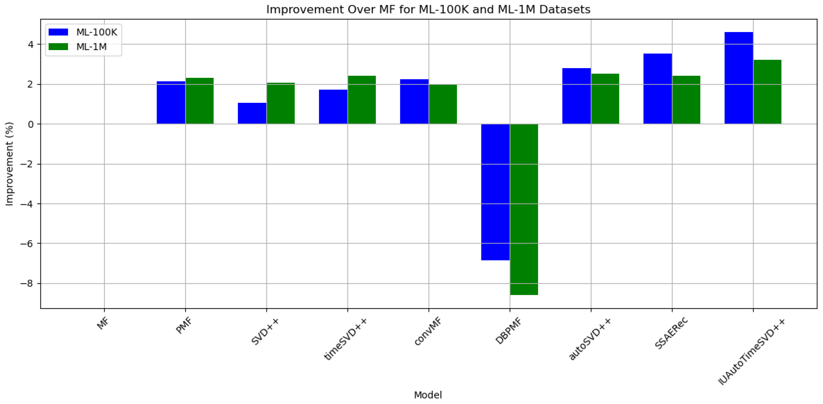
4.6.2. Improvement Analysis

To quantify the effectiveness of the IUAutoTimeSVD++ model over the baseline models, we compute the improvements of our model and other baseline models compared to the baseline model MF [14] as shown in Figure 2:

Indeed, based on the improvement analysis results in Figure 2, it is evident that the IUAutoTimeSVD++ model consistently outperforms the baseline models. The improvement plot clearly shows that the bars for IUAutoTimeSVD++ are above the horizontal dashed line (representing the baseline performance) for both datasets. This indicates that the IUAutoTimeSVD++ model achieves a lower RMSE value as compared to the baseline models, indicating superior predictive accuracy in making recommendations. The improvements showing that the integration of temporal dynamics and user–item features extracted through the contractive autoencoder leads to enhanced recommendation performance. The finding that IUAutoTimeSVD++ outperforms the baselines is valuable, as it demonstrates the effectiveness of the proposed model in addressing the limitations of traditional matrix factorization models through the use of CAE to extract user–item features. It also indicates that the inclusion of temporal dynamics and user–item features enhances the accuracy recommendation.

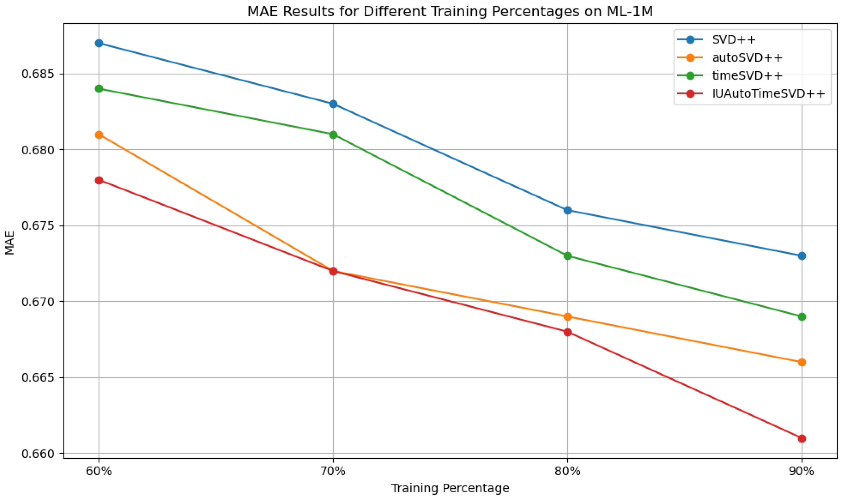
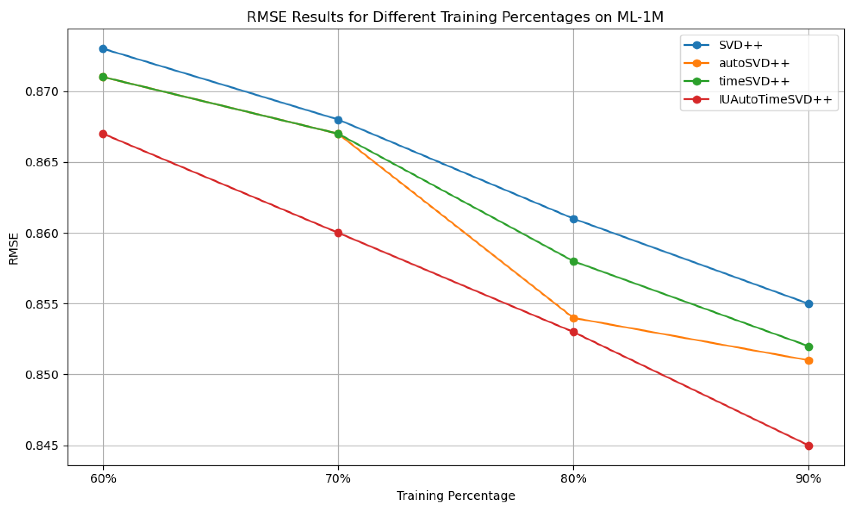
4.7. Effectiveness Study of Training Size Impact

To study the impact of the training/test dataset size, we conducted many experiments using several values of training size $\{60,70,80,90\}$. The results are presented in

Table 10. RMSE and MAE experimental results for different training percentages on ML-100K.

Dataset	Training	Metrics	SVD++	autoSVD++	timeSVD++	IUAutoTimeSVD++
ML-100K	90%	RMSE	0.925	0.909	0.919	0.892
		MAE	0.731	0.712	0.724	0.699
	80%	RMSE	0.943	0.925	0.929	0.912
		MAE	0.742	0.726	0.733	0.716
	70%	RMSE	0.935	0.920	0.939	0.915
		MAE	0.739	0.725	0.742	0.720
	60%	RMSE	0.944	0.938	0.941	0.936
		MAE	0.744	0.738	0.741	0.738

and

Table 11. RMSE and MAE experimental results for different training percentages on ML-1M.

Dataset	Training	Metrics	SVD++	autoSVD++	timeSVD++	IUAutoTimeSVD++
ML-1M	90%	RMSE	0.855	0.851	0.852	0.845
		MAE	0.673	0.666	0.669	0.661
	80%	RMSE	0.861	0.854	0.858	0.853
		MAE	0.676	0.669	0.673	0.668
	70%	RMSE	0.868	0.859	0.867	0.860
		MAE	0.683	0.672	0.681	0.672
	60%	RMSE	0.873	0.871	0.871	0.867
		MAE	0.687	0.681	0.684	0.678

:

We complement the effectiveness study results presented in Table 10 and Table 11 with visual representations in the following figures:

Effectiveness Study Results Analysis

Based on the comprehensive analysis of performance results across different test ratio configurations, as illustrated in Table 10 and Table 11 (Figure 3 and Figure 4) it becomes evident that the IUAutoTimeSVD++ model consistently outperforms other models. This is reflected in its superior accuracy, with lower values of RMSE and MAE on both the ML-100K and ML-1M datasets. Notably, the IUAutoTimeSVD++ model exhibits remarkable performance regardless of the proportion of data used for testing (10%, 20%, 30%, or 40%). It consistently demonstrates robustness and effectiveness in making accurate predictions and recommendations across various testing scenarios. Additionally, it is noteworthy that all the compared models achieve a better accuracy when utilizing a higher training ratio (90% of the data), as evidenced by lower RMSE values for both the ML-100K and ML-1M datasets. This observation emphasizes the importance of allocating more resources for the training phase. A higher training ratio allows the model to learn from a more extensive and representative portion of the data.

4.8. Ablation Study

In this subsection, we conduct an ablation study to dissect and scrutinize the key components influencing our model’s performance. Specifically, we isolate and analyze the impact of three critical factors: the temporal aspect, user features, and item features. By systematically varying or removing each component individually, we aim to discern their respective contributions to the overall model efficacy.

Table 12. Ablation Study on Model Components.

Model	Time	Item Features	User Features
timeSVD++	✔
I-AutoTimeSVD++	✔	✔
U-AutoTimeSVD++	✔		✔
IU-autoSVD++		✔	✔
IUAutoTimeSVD++	✔	✔	✔

enumerates the components employed in each variant examined in our ablation study:

4.8.1. Results

The results of the ablation study on both datasets are presented in

Table 13. Ablation study results for ML-100K.

Model	RMSE	MAE
timeSVD++	0.919	0.724
I-AutoTimeSVD++	0.896	0.704
U-AutoTimeSVD++	0.896	0.704
IU-autoSVD++	0.909	0.712
IUAutoTimeSVD++	0.892	0.699

and

Table 14. Ablation study results for ML-1M.

Model	RMSE	MAE
timeSVD++	0.852	0.669
I-AutoTimeSVD++	0.851	0.667
U-AutoTimeSVD++	0.845	0.662
IU-autoSVD++	0.851	0.666
IUAutoTimeSVD++	0.845	0.661

:

Based on analysis of the ablation study results in Table 13 and Table 14, the IUAutoTimeSVD++ model, which encompasses all three components (time, user, and item features), demonstrated the lowest RMSE and MAE values. This performance advantage signifies that IUAutoTimeSVD++ outperformed the other variants concerning predictive accuracy. The ablation study provided valuable insights into the significance of each component within the model. The presence of time, user, and item features working together smoothly enhanced the model’s ability to make the predictions more accurate. Notably, the results indicate that user and item features hold more importance than the time factor in predicting ratings. The integration of user features had a more substantial impact on the model’s performance compared to incorporating item features. Moreover, it was observed that leveraging only the user features yielded better accuracy.

4.8.2. Improvement Ablation Study Analysis

To gain a comprehensive understanding of the performance improvement of each variant of the model, we assess the improvement of all variants in comparison to the baseline model, timeSVD++. In this analysis, we calculate the difference in performance metrics (e.g., RMSE and MAE) between each variant and the baseline. This allows us to quantify how much better or worse each variant performs relative to the baseline. The results are illustrated in Figure 5 and Figure 6:

In light of analysis of the improvement plots (Figure 5 and Figure 6) the IUAutoTimeSVD++ model consistently outperforms the other variants and the baseline model timeSVD++, demonstrating its effectiveness in improving the recommendation accuracy. The inclusion of both user and item features (IUAutoTimeSVD++) appears to be more beneficial than including either user or item features alone (I-AutoTimeSVD++ and U-AutoTimeSVD++). The IU-autoSVD++ variant, which does not include the time component, performs slightly worse compared to the IUAutoTimeSVD++ model, suggesting that consideration of the temporal dynamics is essential for enhancing the model’s prediction accuracy. Overall, the ablation study highlights the significance of each component in the proposed IUAutoTimeSVD++ model and underscores its superiority in making accurate predictions and recommendations on both ML-100K and ML-1M datasets. The results provide valuable insights into the model’s effectiveness and the importance of incorporating user, item, and temporal features to tackle the sparsity problem and enhance the matrix factorization model for recommender systems.

4.9. Experimental Analysis on Sparse Synthetic Dataset: Subsampling MovieLens Data

We delve into the experimental analysis conducted on a synthetic dataset derived from the MovieLens dataset. The synthetic dataset is generated through subsampling (selecting the 30% of the user reviews), where a fraction of the original MovieLens data is retained to create a sparser version. This process allows us to explore the behavior of recommendation algorithms under varying degrees of data sparsity and evaluate the robustness of our proposed model, mimicking real-world scenarios with limited interaction data.

Table 15. Dataset Statistics.

Dataset	# Interactions	# Users	# Items	Sparsity (%)
Synthetic MovieLens 100K	30,000	943	1499	98.09
Synthetic MovieLens 1M	300,063	6040	3531	98.76

present the statistics of the synthetic datasets (ML-100K and ML-1M) after resampling and only selecting (30%) of reviews.

In our evaluation of compared recommendation models on synthetic datasets derived from the original MovieLens datasets (ML-100K and ML-1M) by retaining only 30% of ratings, we aimed to assess the models’ adaptability and performance under sparse data conditions. The results indicate that IUAutoTimeSVD++ consistently demonstrates robust performance on the synthetic datasets, despite the lower data density. With RMSE scores of $0.959$ on Synthetic ML-100K and $0.906$ on Synthetic ML-1M as shown in

Table 16. RMSE results for synthetic ML-100K and ML-1M Datasets.

Model	Synthetic ML-100K RMSE	Synthetic ML-1M RMSE
MF	0.962	0.915
SVD++	0.961	0.913
timeSVD++	0.959	0.909
autoSVD++	0.961	1.010
IUAutoTimeSVD++	0.959	0.906

, IUAutoTimeSVD++ exhibits resilience and effectiveness in capturing underlying user–item interactions even with limited rating information. This highlights its ability to generalize well and maintain performance across varying data densities. However, it is important to note that while IUAutoTimeSVD++ excelled on the synthetic datasets, the evaluation was limited to this model due to the unavailability of code for other baseline models. As a result, the performance of these models under sparse conditions remains unexplored. Nonetheless, the strong performance of IUAutoTimeSVD++ on the synthetic datasets underscores its potential for real-world applications where data sparsity is a challenge due to limited user–item interactions. This analysis provides valuable insights into how these models fare when faced with reduced data density, which is common in real-world applications.

5. Conclusions

We proposed IUAutoTimeSVD++, a novel hybrid model extending the temporal dynamic latent factor model timeSVD++ by incorporating user side information and item features. Our primary goal was to tackle the sparsity issue in matrix factorization and ensure a dynamic rating prediction mechanism. The proposed model leverages a contractive autoencoder to combine pre-trained item and user features, enabling a robust representation of the input features. Our experimental results have shown that IUAutoTimeSVD++ outperforms several baseline models, including those based on time and latent factors. The model’s superior performance validates the effectiveness of incorporating user and item features and the temporal dynamics into the rating prediction process. As a future direction, we aim to enhance the model’s capability in capturing short-term interactions. Currently, IUAutoTimeSVD++ focuses on modeling long-term user tastes, but incorporating short-term preferences, such as session-based interactions or recent user behaviors, is essential for providing more timely and accurate recommendations. To achieve this, we plan to adopt a recurrent neural network (RNN) and techniques like gated recurrent units (GRUs) [25] and long short-term memory (LSM) [26], which are adept at capturing sequential patterns in user–item interactions. Another promising research direction combining contrastive learning (CL) framework for matrix factorization models—where positive user–item interactions are contrasted with negative interactions to learn more informative latent representations inspired by some recent research such as [20] and the contractive autoencoder (CAE) providing a compact and dense representations of user and item features—could focus on developing a novel recommendation model that leverages the strengths of each technique. Additionally, we intend to explore additional rich features, such as visual and textual item attributes, to create a more comprehensive and personalized recommendation system. Moreover, we plan to explore parallel and distributed computing models like DSGD (distributed stochastic gradient descent) [27] to enhance the model’s efficiency and scalability for handling larger datasets.

References

1. Ricci, F.; Rokach, L.; Shapira, B. (Eds.) Recommender Systems Handbook, 2nd ed.; Springer: New York, NY, USA, 2015. [Google Scholar] [CrossRef]
2. Ekstrand, M.D.; Riedl, J.T.; Konstan, J.A. Collaborative Filtering Recommender Systems. Found. Trends Hum.-Comput. Interact. 2011, 4, 81–173. [Google Scholar] [CrossRef]
3. Bell, R.M.; Koren, Y. Lessons from the Netflix Prize Challenge. SIGKDD Explor. Newsl. 2007, 9, 75–79. [Google Scholar] [CrossRef]
4. Rendle, S.; Krichene, W.; Zhang, L.; Anderson, J. Neural Collaborative Filtering vs. Matrix Factorization Revisited. arXiv 2020, arXiv:2005.09683. [Google Scholar]
5. Anelli, V.W.; Bellogín, A.; Di Noia, T.; Pomo, C. Reenvisioning Collaborative Filtering vs. Matrix Factorization. In Proceedings of the Fifteenth ACM Conference on Recommender Systems, Amsterdam, The Netherlands, 27 September–1 October 2021; pp. 521–529. [Google Scholar]
6. Zhang, S.; Yao, L.; Sun, A.; Tay, Y. Deep Learning Based Recommender System: A Survey and New Perspectives. ACM Comput. Surv. 2019, 52, 1–38. [Google Scholar] [CrossRef]
7. Mu, R. A Survey of Recommender Systems Based on Deep Learning. IEEE Access 2018, 6, 69009–69022. [Google Scholar] [CrossRef]
8. Zhang, S.; Yao, L.; Xu, X. AutoSVD++: An Efficient Hybrid Collaborative Filtering Model via Contractive Auto-encoders. In Proceedings of the 40th International ACM SIGIR Conference on Research and Development in Information Retrieval, Tokyo, Japan, 7–11 August 2017; pp. 957–960. [Google Scholar] [CrossRef]
9. Kim, D.; Park, C.; Oh, J.; Lee, S.; Yu, H. Convolutional Matrix Factorization for Document Context-Aware Recommendation. In Proceedings of the 10th ACM Conference on Recommender Systems RecSys ’16, New York, NY, USA, 15–19 September 2016; pp. 233–240. [Google Scholar] [CrossRef]
10. Zhang, Y.; Zhao, C.; Chen, M.; Yuan, M. Integrating Stacked Sparse Auto-Encoder Into Matrix Factorization for Rating Prediction. IEEE Access 2021, 9, 17641–17648. [Google Scholar] [CrossRef]
11. Azri, A.; Haddi, A.; Allali, H. autoTimeSVD++: A Temporal Hybrid Recommender System Based on Contractive Autoencoder and Matrix Factorization. In Proceedings of the Smart Applications and Data Analysis—4th International Conference, SADASC 2022, Marrakesh, Morocco, 22–24 September 2022; Hamlich, M., Bellatreche, L., Siadat, A., Ventura, S., Eds.; Springer: Berlin/Heidelberg, Germany, 2022; Volume 1677, Communications in Computer and Information Science. pp. 93–103. [Google Scholar] [CrossRef]
12. Koren, Y. Collaborative filtering with temporal dynamics. In Proceedings of the KDD09: The 15th ACM SIGKDD International Conference on Knowledge Discovery and Data Mining, Paris, France, 28 June–1 July 2009; pp. 447–456. [Google Scholar]
13. Rifai, S.; Vincent, P.; Muller, X.; Glorot, X.; Bengio, Y. Contractive auto-encoders: Explicit invariance during feature extraction. In Proceedings of the 28th International Conference on International Conference on Machine Learning ICML’11, Madison, WI, USA, 28 June–2 July 2011; pp. 833–840. [Google Scholar]
14. Koren, Y.; Bell, R.; Volinsky, C. Matrix Factorization Techniques for Recommender Systems. Computer 2009, 42, 30–37. [Google Scholar] [CrossRef]
15. He, R.; McAuley, J. VBPR: Visual Bayesian Personalized Ranking from Implicit Feedback. arXiv 2015, arXiv:1510.01784. [Google Scholar] [CrossRef]
16. Abdollahi, B.; Nasraoui, O. Explainable Matrix Factorization for Collaborative Filtering. In Proceedings of the 25th International Conference Companion on World Wide Web WWW ’16 Companion, Geneva, Switzerland, 11–15 April 2016; pp. 5–6. [Google Scholar] [CrossRef]
17. He, X.; Liao, L.; Zhang, H.; Nie, L.; Hu, X.; Chua, T.S. Neural Collaborative Filtering. In Proceedings of the 26th International Conference on World Wide Web WWW ’17, Perth, Australia, 3–7 April 2017; pp. 173–182. [Google Scholar] [CrossRef]
18. Mnih, A.; Salakhutdinov, R.R. Probabilistic Matrix Factorization. In Advances in Neural Information Processing Systems 20; Platt, J.C., Koller, D., Singer, Y., Roweis, S.T., Eds.; Curran Associates, Inc.: Red Hook, NY, USA, 2008; pp. 1257–1264. [Google Scholar]
19. Li, K.; Zhou, X.; Lin, F.; Zeng, W.; Alterovitz, G. Deep Probabilistic Matrix Factorization Framework for Online Collaborative Filtering. IEEE Access 2019, 7, 56117–56128. [Google Scholar] [CrossRef]
20. Ren, X.; Xia, L.; Zhao, J.; Yin, D.; Huang, C. Disentangled contrastive collaborative filtering. In Proceedings of the 46th International ACM SIGIR Conference on Research and Development in Information Retrieval, Taipei, Taiwan, 23–27 July 2023; pp. 1137–1146. [Google Scholar]
21. Wang, Y.; Wang, X.; Huang, X.; Yu, Y.; Li, H.; Zhang, M.; Guo, Z.; Wu, W. Intent-aware Recommendation via Disentangled Graph Contrastive Learning. In Proceedings of the Thirty-Second International Joint Conference on Artificial Intelligence, IJCAI-2023, Macao, 19–25 August 2023. [Google Scholar] [CrossRef]
22. Bank, D.; Koenigstein, N.; Giryes, R. Autoencoders. arXiv 2021, arXiv:2003.05991. [Google Scholar]
23. Harper, F.M.; Konstan, J.A. The movielens datasets: History and context. Acm Trans. Interact. Intell. Syst. 2015, 5, 1–19. [Google Scholar] [CrossRef]
24. Aggarwal, C.C. Recommender Systems: The Textbook, 1st ed.; Springer: Berlin/Heidelberg, Germany, 2016. [Google Scholar]
25. Cho, K.; Van Merriënboer, B.; Gulcehre, C.; Bahdanau, D.; Bougares, F.; Schwenk, H.; Bengio, Y. On the properties of neural machine translation: Encoder-decoder approaches. arXiv 2014, arXiv:1409.1259. [Google Scholar]
26. Hochreiter, S.; Schmidhuber, J. Long short-term memory. Neural Comput. 1997, 9, 1735–1780. [Google Scholar] [CrossRef] [PubMed]
27. Gemulla, R.; Nijkamp, E.; Haas, P.J.; Sismanis, Y. Large-scale matrix factorization with distributed stochastic gradient descent. In Proceedings of the 17th ACM SIGKDD International Conference on Knowledge Discovery and Data Mining, San Diego, CA, USA, 21–24 August 2011; pp. 69–77. [Google Scholar] [CrossRef]
Figure 1. IUAutoTimeSVD++ model architecture.
Information 15 00204 g001
Figure 2. Improvement in RMSE for IUAutoTimeSVD++ model over baseline (MF) on ML-100K and ML-1M Datasets.
Information 15 00204 g002
Figure 3. RMSE results for different training percentages on ML-100K.
Information 15 00204 g003
Figure 4. RMSE results for different training percentages on ML-1M.
Information 15 00204 g004
Figure 5. Improvement in ablation study results for ML-100K dataset.
Information 15 00204 g005
Figure 6. Improvement in ablation study results for ML-1M dataset.
Information 15 00204 g006