Abstract
Workload management is a cornerstone of contemporary human resource management with widespread applications in private and public sectors. The challenges in human resource management are particularly pronounced within the public sector: particularly in task allocation. The absence of a standardized workload distribution method presents a significant challenge and results in unnecessary costs in terms of man-hours and financial resources expended on surplus human resource utilization. In the current research, we analyze how to deal with the “race condition” above and propose a dynamic workload management model based on the response time required to implement each task. Our model is trained and tested using comprehensive employee data comprising 450 records for training, 100 records for testing, and 88 records for validation. Approximately 11% of the initial data are deemed either inaccurate or invalid. The deployment of the ANFIS algorithm provides a quantified capability for each employee to handle tasks in the public sector. The proposed idea is deployed in a virtualized platform where each employee is implemented as an independent node with specific capabilities. An upper limit of work acceptance is proposed based on a documented study and laws that suggest work time frames in each public body, ensuring that no employee reaches the saturation level of exhaustion. In addition, a variant of the “slow start” model is incorporated as a hybrid congestion control mechanism with exceptional outcomes, offering a gradual execution window for each node under test and providing a smooth and controlled start-up phase for new connections. The ultimate goal is to identify and outline the entire structure of the Greek public sector along with the capabilities of its employees, thereby determining the organization’s executive capacity.
1. Introduction
The public sector faces mounting pressure to transform its operations and service delivery mechanisms in an era marked by rapid technological advancements and evolving societal demands. The need for agility, responsiveness, and efficiency within government agencies has never been more pressing [1]. Central to addressing these challenges is the development and implementation of a robust dynamic workload management system (DWMS) tailored to the unique demands of the public sector.
Traditional public administration systems often struggle to adapt to changing circumstances, leading to inefficiencies, delays, and suboptimal resource allocation [2]. In addition, they lack independent performance assessments, while reformation approaches must be adapted to evolving circumstances [3]. In this context, a DWMS emerges as a critical tool for enhancing the performance of public sector organizations by optimizing work distribution, resource allocation, and service delivery processes in real time. The current paper analyzes the conceptualization, design, and practical implementation of such a system, aiming to bridge the gap between theory and practice, as well as seeks to explore the development of a DWMS as a strategic imperative for the public sector. The significance of this study lies in its potential to transform how government agencies operate, enabling them to respond swiftly to emerging challenges, allocate resources judiciously, and enhance overall service quality. By providing a comprehensive understanding of DWMS design and implementation in the public sector, this research contributes to the body of knowledge on public administration and management. Workload distribution was always the “Achilles heel” of any system related to human resource management. The current situation is characterized by an overabundance of public sector employees, many without the necessary training. At the same time, it is not uncommon for individuals to become overwhelmed by the high volume of work, leading to delays in completing several tasks. Consequently, the quality of these tasks may suffer as they are rushed to meet deadlines. Highly skilled employees are overloaded with tasks that cannot be handled in their daily schedule, resulting in overtime and physical and mental problems [4,5]. On the other hand, underutilized human resources, due to a subjective assessment of lack of specialization, do not undertake jobs, resulting in the operation of two-speed services and the gradual cessation of all activities.
The existing literature reveals a significant gap in research regarding the development and implementation of DWMSs in the public sector. Although related concepts and theories have been explored, two critical aspects remain unaddressed. First, existing management systems often rely on performance indicators and assessments based on supervisors’ opinions rather than productivity factors. This oversight limits the objectivity and effectiveness of workload management. Second, there is a lack of a holistic approach to modeling the potential efficiency of public bodies based on employee efficiency. This gap hinders the ability to comprehensively evaluate and enhance organizational performance. Furthermore, the selection of the ANFIS algorithm as the candidate for producing the Capacity Factor for each employee was based on pre-analysis with actual data and is supported by a robust theoretical framework. Thus, there is a clear need for comprehensive analysis and practical guidance on designing and implementing DWMSs that address these gaps. The current investigation sheds light on various aspects of the problem by highlighting task boundary management.
The paper is organized into several sections, including a literature review of relevant concepts and theories, a discussion of the critical components of a DWMS, and case studies illustrating successful implementations. It concludes by offering insights into the potential future developments in dynamic workload management in the public sector.
In summary, current research promotes a dynamic workload management system’s pivotal role in enhancing public sector organizations’ efficiency and effectiveness. By addressing the challenges and opportunities inherent in such a system, we aim to provide a comprehensive resource for policymakers, directors, and researchers invested in the future of public administration.
2. Related Work and Contributions
Workload management in the public sector has not been extensively reported, although researchers have attempted to outline the proposed topic. A quite exciting approach was initiated by Michalopoulos et al. [6], where a four-level factor profile was utilized to produce the correlation between the hard skills and the Capacity Factor (CF) to determine each employee’s efficiency. This initial deployment was further deployed in the research by Giotopoulos et al. [7], where results illustrated the significant impact of work experience in the private sector compared to the public sector on the value of the Capacity Factor. ANFIS was selected due to its ability to learn and represent complex nonlinear relationships effectively. While the deployment of neural networks has demonstrated remarkable predictive capabilities, a large amount of information in the public domain remains unexploited. Therefore Theodorakopoulos et al. [8,9] showed the use of big data and machine learning for predicting valuable information in many fields of modern business that could be applied to any public body. The study of Adams et al. [10] suggests that for sustainability reporting to become widespread in the public sector, it may require mandatory adoption or a shift toward competitive resource allocation based on sustainability performance. However, these conclusions are subject to potential limitations, and future research should explore the role of regulatory environment congruence in sustainability performance. The importance of intangible assets (IAs) and intellectual capital (IC) was also highlighted by Boj et al. [11], who introduced a methodology using an analytic network process (ANP). Regarding productivity in the public sector, the use and usefulness of corresponding performance measures are considered vital [12]. Arnaboldi et al. [13] proposed leveraging complexity theory to address the intricacies of public sector performance management, taking into account performance management, exploring the applicability of complexity theory to public service managers’ everyday tasks, and conducting a holistic evaluation including public managers. Gunarsih et al. [14] emphasized the importance of comprehensive performance measurement by integrating the balanced scorecard (BSC) method along with system dynamics (SD) modeling to capture complex interactions. On the other hand, Bruhn et al. [15] introduced a multi-level approach to understanding frontline interactions within the public sector and demonstrated the value of applying conversation analysis methods to investigate how policies and rules are applied, negotiated, and reshaped during those interactions. Indicators such as allocation, distribution, and stabilization have been analyzed, leading to defined measurements of public sector performance (PSP) and efficiency (PSE), giving an advantage to smaller public bodies [16].
There is still an ongoing debate regarding measuring productivity in public services. This debate suggests that we are currently in a phase characterized by testing various approaches, making it challenging to draw meaningful comparisons.
When discussing and assessing the performance of public services, it is crucial to clearly distinguish between various aspects of public service performance, such as productivity, efficiency, and effectiveness, and how working time flexibility affects those factors. Integrating working time flexibility into this strategy can contribute positively to productivity but has various impacts due to the range of measures implemented. The manner of implementation and collective influence affect working conditions, and work–life balance and other relevant factors are emphasized [17]. A measurable dimension that will determine the efficiency of a civil servant is still missing. Instead, government outputs typically encompass complex social outcomes that are challenging to precisely delineate and often exhibit multidimensional and interconnected characteristics [18].
A challenge that arises when considering the private sector when comparing public and private sector efficiency is the achievement of complete comparability, which would allow for an adequate evaluation of each. Even a cursory analysis reveals that the public and private sectors are not interchangeable. Their objectives diverge significantly, with the private sector primarily focused on profit generation. At the same time, the public sector seeks economic gains and the attainment of social benefits, with a primary mission of ensuring the public’s well-being. Private sector projects are primarily driven by the pursuit of economic benefits: often with limited attention to social and environmental concerns. However, in contemporary times, many companies are gradually shifting their mindsets and are striving to integrate social responsibility alongside profit generation. Conversely, public projects may prioritize social benefits over economic gains [19].
The relationship between outcomes or outputs, as the literature refers to them, and inputs or efforts determines efficiency. While this relationship may seem straightforward, practical implementation often proves otherwise. Identifying and measuring inputs and outputs in the public sector is generally a challenging endeavor.
How is productivity related to working hours? Definitely, increasing working time does not correspond to a proportional increase in productivity due to fatigue, which is the most crucial parameter in the equation [20,21,22]. On the other hand, factors such as wages, work arrangements, job content, IT skills, working conditions, health, stress, and job satisfaction significantly contribute to employee productivity [23]. In contrast, incentives for companies to adopt and expand flexible working time arrangements, like flextime and working time accounts, can improve morale, individual performance, and overall company productivity and sustainability [24].
An interesting approach elucidates a path to augmenting production efficiency by implementing a work-sharing methodology. Workforce reduction is achieved by meticulously assessing cycle times per head, as organized by a process [25].
While it is relatively straightforward to measure inputs in terms of physical units, such as the number of employees or hours worked, or in financial terms, defining and quantifying outputs presents more significant challenges. This is due to the diverse perspectives that consumers may have, whether they are viewed as end-users or representatives of society at large.
Furthermore, additional complexities arise when it comes to defining and measuring the outcomes of public services. External factors such as individual behavior, culture, and social norms can significantly influence the final results, making it a multifaceted and intricate process [26].
In analogous investigations aimed at forecasting student performance through prior academic attainments, algorithms including naive Bayes, ID3, C4.5, and SVM were utilized, with particular emphasis on their applicability and analyses concerning students. The evaluation of these algorithms centered on metrics such as accuracy and error rates [27].
Aligned with the prevailing tendency towards incorporating AI in human resource management, Chowdhury et al. [28] undertook a systematic review of AI research in HRM and delineated key themes such as AI applications, collective intelligence, and AI drivers and barriers. While the existing literature predominantly concentrates on AI applications and their associated advantages, a research gap exists regarding collective intelligence, AI transparency, and ethical considerations. The paper introduces an AI capability framework for organizations and suggests research priorities, including validating the framework, assessing the impact of AI transparency on productivity, and devising knowledge management strategies for fostering AI–employee collaboration. It underscores the necessity for empirical studies to comprehensively evaluate the effects of AI adoption.Use of machine learning combined with metrics such as mean absolute error, mean squared error, and R-squared have been widely used lately for evaluating employee performance [29]. Alsheref et al. [30] proposed automated model that can predict employee attrition based on different predictive analytical techniques such as random forest, gradient boosting, and neural networks, while Arslankaya, S., focused on employee labor loss, demonstrating the superiority of ANFIS over pure fuzzy logic [31]. In all cases, it was evident that there is a need for a recruitment system that can use artificial intelligence during the hiring procedure to quantify the objectives set by the HR department [32] and move into a more personalized HRM system [33] that provides insight into workload performance of the personnel. The incorporation of artificial intelligence (AI) and machine learning (ML) into business process management (BPM) within organizations and enterprises holds promise for achieving these goals and enhancing performance, innovation procedures, and competitive edges [34].
In continuation of the research defining efficiency to include the measurement and evaluation of workloads, Casner, S.M., and Gore [35] made a quite remarkable approach by highlighting factors such as speed, accuracy, and task analysis and tried to illustrate the performance relation to the quantification of the workloads of pilots. A load-balancing algorithm could analyze and manage the load distributed on any public service in the same way that protocols operate in the IT world. Compared to static ones, dynamic algorithms gather and combine the load information to make decisions for load balancing. Sharifian et al. [36] proposed an approach that involves predicting server utilization and then correcting this prediction using real-time feedback on response time, while Xu and Wang [37] introduced a modified round-robin algorithm designed to enhance web server performance, particularly during periods of transient overload. In the same way, Diao, Y., and Shwartz [38] illustrated the development of autonomic systems for IT service management, aiming to improve service quality while optimizing costs. They employ automated data-driven methodologies encompassing workload management through feedback controllers, workforce management using simulation optimization, and service event management with machine learning models. Real-world examples from a large IT services delivery environment validate the effectiveness of these approaches. The impact of workloads on HR was highlighted by Razzaghzadeh et al., who introduced a novel load-balancing algorithm designed for expert clouds that emphasized both load distribution and efficient task allocation based on a mathematical model. It leverages nature-inspired colorful ants to rank and distinguish the capabilities of human resources (HRs) within a tree-structured site framework. Tasks and HRs are labeled and allocated by super-peer levels using Poisson and exponential distribution probability functions. The proposed method enhances throughput, reduces tardiness, and outperforms existing techniques when tested in a distributed cloud environment [39]. In many research works, multitasking has been considered in order to reduce and effectively cope with workloads. Bellur et al. [40] deployed cognitive theories to understand multitasking’s effects in educational settings, emphasizing students’ technology use. They investigated multitasking’s impact on college GPAs and distinguished multitasking efficacy and additional study time as covariates. The study revealed that multitasking during class negatively affects GPA, surpassing the influence of study time. Rubinstein et al. [41] also indicated that, regardless of task type, people experienced time loss when transitioning from one task to another. Additionally, the duration of these time costs escalated with the intricacy of the tasks, resulting in notably longer switching times between more complex tasks. Moreover, the time costs were higher when individuals shifted to less familiar tasks. In theory and experimentation, significant advancements have been achieved concerning how cognitive control affects immediate task performance. Increased cognitive control requirements during encoding consistently lead to a deceleration in performance and an uptick in error rates according to Reynolds [42] and Meier and Rey-Mermet [43], while Muhmenthaler and Meier proved in their research that task switching consistently impaired memory across all experiments conducted [44]. Mark et al. [45] pointed out in their study that task interruptions “cost” an average of 23 min and 15 s to get back to the task. On average, individuals who frequently switch tasks experience a loss of focus for just tens of minutes each time. Consequently, their efficiency is reduced by approximately 20–40% [41].
However, the aforementioned approaches lack a reliable management system for evaluating employee productivity. Traditional evaluation systems, characterized by subjectivity from experts and bureaucratic processes, fall short in providing adequate performance appraisals. This inadequacy underscores the urgent need for transformative strategies in public administration, especially in the context of the ongoing digital transformation era. This research emphasizes the integration of objective efficiency assessment mechanisms, moving away from traditional systems that rely on domain experts and their inherent subjectivity. Introducing a time variant factor that measures the execution of each task by a central HRMS is an innovative approach. Therefore, the novel contribution of this study extends further by utilizing the capabilities of employees within each public body to achieve a balanced workload network. Merely assessing and classifying employees is insufficient without a strategic framework that demonstrates how to effectively deploy those results.
3. Methodology
3.1. Tasks and Capacity Factor
Every country has laws defining the number of and duration of time spent on breaks for each employee. In Greece, if the continuous daily working hours exceed 2 h, public servants are entitled to a minimum 15 min break, during which they can temporarily leave their workstations. This break cannot be accumulated at the start or end of the workday, as per the adjustments made by Law 4808 of 2021, Article 56, and the 540/2021 decision of the Supreme Court, while the required skill set for a public servant is based on decision No. 540/2021 from the Greek Council of State according to Council Directive 90/270/EEC.
We base our hypothesis on the fact that each employee possesses a unique set of complex skills that influence their ability to complete tasks within a specified time frame, referred to as the “Time Factor”. As each employee is bound to a specific profile, indicated by Michalopoulos et al. [6], each individual can be treated as a separate node with designated skills for its properties, leading to a unique Time Factor. As such, for every employee or node, a specific Time Factor is assigned based on their skills and is represented by factors K1 through K4 according to Michalopoulos et al. [6].
The selected factors are
- K1: academic skills (number of Bachelor’s degrees, availability of Master’s degree, certification from the National School of Public Administration, and PhD diploma);
- K2: working experience in the public sector (number of years, with a maximum number of 35, plus type of responsibility);
- K3: working experience in the private sector (number of years, with a maximum number of 35, plus type of responsibility);
- K4: Age in number of years within the range of 20–67.
Tasks are categorized according to complexity into , indicating a proportional increase in their execution times, and is considered the task with minimum complexity. Therefore, = task weight x, which indicates the complexity of each task as measured in a specified time unit , which can be mins, hours, etc., in terms of the metric.
When a task is allocated to employee , the associated timer is triggered and continues until the task is completed.
For as long as the timer runs, each profile is assigned with various tasks, but all of them will be dependent on the base . So for a given number of samples n, the Time Factor is denoted as the mean value of all timers of tasks proportional to .
Therefore, for any given profile and task ,
In continuation of the previous assumptions, each employee profile has a unique capability to accomplish tasks per time unit TU; this is designated as the Capacity Factor. Therefore,
So from the assumptions above, it is deducted that: , where is the skill identification for each employee according to Michalopoulos et al. [6].
Figure 1 illustrates the procedure, which involves a multi-step approach to regulate load control in a network using four factors, through , as inputs. These steps are outlined and explained as follows: Input to ANFIS: The four factors , , , and are utilized as inputs to the adaptive neuro-fuzzy inference system (ANFIS). The role of the ANFIS here is to process these input factors and produce an output termed the Time Factor. Derivation of Capacity Factor: Once the Time Factor is obtained from the ANFIS, it serves as an intermediary variable for the calculation of the Capacity Factor. The Capacity Factor is a critical metric that quantifies the efficiency of the node within each public body. Load control mechanism: Each node within the network utilizes the derived Capacity Factor to regulate its load. This process is part of a load control mechanism, wherein the nodes adjust their operational loads based on the Capacity Factor to optimize overall network performance. The Capacity Factor (CF) is mathematically dependent on the four initial factors (K1 to K4). This relationship can be expressed as a function CF = f(K1,K2,K3,K4), indicating that the Capacity Factor is a resultant function of the inputs K1, K2, K3, and K4.
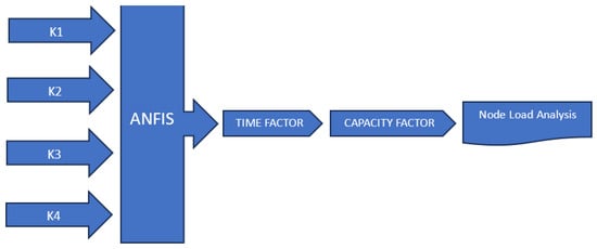
Figure 1.
Illustration of how inputs K1 to K4 contribute to the production of the Capacity Factor.
The public body now consists of a multi-core “equivalent to IT based platform”, where each employee () is a potential CPU “running” at a distinct Capacity Factor. For the rest of the study, each employee will be denoted as (node ) such that:
In the current research, the following primary tasks (Table 1) for areas of interest were identified:

Table 1.
Public body tasks.
Table 2 provides the durations, in minutes, for draft tender design () and international tender design () from 15 distinct profile samples according to Giotopoulos et al. (2023) [7]. is always the baseline for Time Factor calculations on any given profile . The Time Factor Table 2 presented below showcases fifteen sample data records received from the system. It delineates the variations in the time taken to accomplish each sample task. and indicate the samples taken for Tasks and , respectively.
Table 2.
Time Factor table.
3.2. Data Collection and Analysis
The population for this study comprised employees from public sector organizations within the western region of Greece. A stratified random sampling method was employed to ensure representation across different departments and levels of hierarchy. This approach was chosen to capture a diverse range of data and improve the generalizability of the findings. The sample size was determined based on the size of the public body under test, and the maximum range was selected in order to ensure sufficient power to detect meaningful effects. A total of 638 participants were selected for the study. Data were collected from performance records, which provided quantitative measures of efficiency. Surveys were not selected since the subjectivity of each expert could influence the validity of the output results. As far as the data collection instrument is concerned, the primary tools used included performance tracking software that is already being adopted by the ministry of labor in Greece. Data were collected over a period of two years, ensuring consistency in measurements across all participants. Detailed instructions were provided to participants to minimize variability in responses.
The adaptive neuro-fuzzy inference system (ANFIS) algorithm was chosen due to its ability to model complex, nonlinear relationships between input variables (K1 up to K4) and the output variable (the Time Factor, indicating performance capability). The rationale for using the ANFIS lies in its superior capability to learn from data and provide interpretable rules. According to the performance indicators, the gbellmf membership function with the use of a hybrid algorithm was selected due to its low root mean squared error. In comparison with an ANN, linear regression, a support vector machine, and a gradient boosting machine, the ANFIS showed better results in terms of RMSE (root mean squared error) and MAPE (mean absolute percentage error) in a preliminary analysis.
Data analysis was conducted using MATLAB R2022b, which facilitated the implementation of the ANFIS algorithm and performed statistical analyses. To ensure the validity and reliability of the ANFIS model, cross-validation techniques were employed. The dataset was divided into training, testing, and validation subsets to evaluate the model’s performance. Sensitivity analyses were conducted to assess the robustness of the findings.
3.3. Load Control and Loadability
Effective load management across the interconnected nodes is fundamental in every interconnected network that handles traffic. The task acceptance limit (TAL) is introduced as the rate, in , at which each node accepts and executes successful tasks. is defined as hourly, daily, weekly, or monthly (in minutes) depending on the time framework imposed by the public service supervisor and is the remaining time for the execution of tasks in the queue. The rate is adjusted automatically per minute by the load control function. Its maximum value is set based on the Capacity Factor.
So for a period of , where 1 and 1 () are accomplished by , it can be deducted that:
What is important is that the daily time framework is different for each country depending on national laws. For eight hours of work, is mins from (10):
In real-time systems, instantaneous monitoring of processor load is conducted at regular intervals during minuscule time segments. However, the proposed solution deviates from this real-time IT-based monitoring approach since supervisors’ allocated time for a task queue is task-specific and predetermined. This signifies that in our envisaged scenario, the node load () shall be computed by aggregating the weight of each task within the node queue, factoring in the predefined remaining time () for all the tasks in the queue, as shown in Figure 2 below. In addition, is defined as the total time of all tasks the node currently possesses in the buffer queue.
where k is the total number of tasks , and is the remaining time in minutes.

Figure 2.
Node buffer.
is the result of , while is updated every minute. The following Algorithm 1 illustrates the Node Load calculation.
| Algorithm 1 Node Buffer |
|
So in the case of and minutes, all tasks will be executed in a single cycle, leaving the remaining minutes either idle or ready for task reception.
We introduce the term (calculated maximum task acceptance limit), which estimates the rate of tasks, which the system accepts when each node operates at maximum load . is the maximum estimated number of tasks, based on minimum task weight , that can be processed per time unit (Giotopoulos et al. [7]) when the exchange operates at maximum task load (loadability).
So what represents the maximum load capacity for each individual node?
We define loadability as the upper limit for the task load each node Ni can process. The limit is set by (1) and (2) as described above, real time delays, and risk of task deployment due to employee performance; the limit is expressed as a percentage of the total available load.
Therefore, taking into account that every node reaches its maximum operational load without degradation at MaxContinousTime per (ValidBreak + MaxContinousTime), from (1) + (2) + (16):
From a theoretical perspective, it is evident that achieving an optimized distribution of the task workload is essential for reaching the highest level of efficiency in any organizational setting. Ideally, each employee should dedicate approximately 88.89% of their total working time to tasks. When the workload surpasses this upper threshold, it inevitably leads to delays and inefficiencies emanating from the employees.
Load control is a vital mechanism that ensures each node within a system remains within a designated protected load zone, preventing it from being overwhelmed by excessive load beyond its handling capacity. The objective is to guarantee successful task throughput even under conditions in which the load surpasses the predefined limit that the node can effectively manage.
In the absence of a load control function safeguarding the system, throughput would exhibit a sharp decline in efficiency at an early overload stage. To sustain optimal task throughput, it becomes imperative to regulate the system’s load by redistributing tasks appropriately or rejecting tasks proportional to the system’s current load. So what is the connection between stress level due to overload and employee performance?
From Figure 3 above, according to Corbett et al. (2015), it becomes clear that as the level of stress becomes too high, performance decreases [46]. As the task-related load increases, stress on every employee also increases proportionally. Similar to our case, there is a direct dependency between employee performance and load distribution.
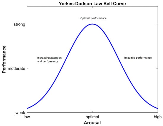
Figure 3.
Yerkes–Dodson law.
Tasks are never executed by following a strict FIFO queue simply because no such mechanism can be applied when working in a dynamic working environment. A dedicated buffer will be kept for all incoming tasks, but the one executed each time will be priority dependent. There are distinct priority scales, , with indicating the highest degree. Thus, as shown in Table 3 for every task with k, :
Table 3.
Node buffer Task Priorities.
Although the list of tasks cannot be considered to be large enough to waste time during indexing, a binary search will be deployed. The worst-case scenario for a binary search occurs when Tki is not in the list and the correct insertion point needs to be determined. In this case, for a total number of n tasks, the worst-case time complexity is , which is still quite efficient for large lists compared to a linear search ().
3.4. Quorum Subscription
In order for any node to be part of the current implementation, it must first be subscribed to the mechanism as seen in Figure 4a, described as capacity provisioning for task distribution (CPFTD).
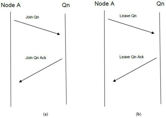
Figure 4.
(a) Join quorum. (b) Leave quorum.
In a public body of n nodes, the quorum consists of all active nodes, as seen in Figure 5, such that:
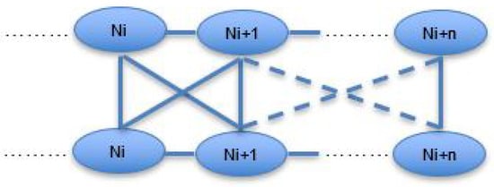
Figure 5.
Qn.
When entering the quorum, each node broadcasts a request to all members of .
As this is a fully distributed solution, no central mechanism provides acknowledgment for entering or leaving the quorum; instead, the acknowledgment is provided by all members of the quorum .
To preserve task redundancy in case of a sudden node “leaving”, each task will be allocated to a primary and secondary node. The selection will be based on a hash algorithm that uniquely selects the primary and secondary nodes. For the purpose of the current research, no failover scenario will be described extensively.
As can be seen from Figure 6, each task ID is allocated on a primary and a secondary node and for the active and passive sections, respectively. In this way, for each receiving task, e.g., for node , the active buffer of primary node will be responsible for task completion. In case of failover on , on the secondary node passive buffer on node will be triggered and transferred to the active side when possible without pushing the load levels above loadability . Node load is only committed on the active buffer of each node.
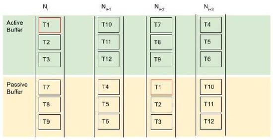
Figure 6.
Task allocation on each node for 12 tasks.
3.5. Slow Start—User History
Each subscribing node undergoes a gradual ramp-up known as a “slow start”. During this phase, nodes are not immediately allocated the total capacity derived from the Capacity Factor within the initial interval. Instead, they are initially granted only a partial percentage of the required capacity. Following this initial phase, a predefined number of intervals, denoted by HISTORYSIZE, is allowed to elapse. Upon completing this specified historical period, the node is regarded as “well-known”. Consequently, the node is granted access to the full capacity as indicated by the Capacity Factor, marking the transition from the slow start phase to full capacity provisioning.
The outlined approach is deemed essential due to the inherent uncertainty in each node’s behavior: specifically, its ability to utilize the capacity indicated by the Capacity Factor effectively. Moreover, it aims to mitigate potential oscillations, given that distinct nodes exert varying impacts on the node load, and this impact is not linearly correlated with reported task usage.
To operationalize this strategy, the capacity granted to a user is initially set at a percentage calculated as HISTORY. During each fetch interval, HISTORY is incremented by one TU. As HISTORY gradually approaches the predefined HISTORYSIZE value, the user’s offered capacity increases proportionally until it reaches the full available capacity once HISTORY equals HISTORYSIZE.
The proposed approach is exemplified in the following illustrative scenario:
Assume Node A sends tasks TWi to be deployed by Node B, while Node B acknowledges every received task. If Node B is new in the “quorum”, it must receive only the minimum of the tasks at the first interval, while it must be granted the total amount after X intervals.
For this reason, the following Algorithm 2 applies to Node A:
At the same time, the following Algorithm 3 applies to target Node B:
| Algorithm 2 Node A |
|
| Algorithm 3 Node B |
|
3.6. Node Capabilities
When capacity is allocated to a set of nodes characterized by relatively consistent behavior, the system gradually approaches a state of loadability over successive intervals. This incremental progression ensures a measured and stable transition toward optimal performance.
A critical threshold is defined to maintain operational stability: the maximum theoretical verge of the node load, set at LDBN. If the task acceptance rate remains below this predetermined threshold, tasks can be accepted and processed without hindrance. However, the system initiates a response mechanism when the task acceptance rate approaches or surpasses the node load value.
In such cases, when the incoming task rate exceeds the node load value, the node accumulates tasks. Ultimately, suppose the task rate persists at this elevated level, exceeding the specified loadability threshold. In that case, tasks over this limit will be, regrettably, rejected, ensuring node efficiency and optimal performance within defined boundaries.
A comprehensive understanding of diverse node profiles and their respective capabilities is essential to accurately determine the node load value. This arises from the system’s overarching design approach, which is intentionally crafted to be versatile and applicable to all node profiles, thereby facilitating the uniform application of capacity provisioning for task distribution (CPFTD).
At the core of this methodology is the Capacity Factor (CF). This metric is fundamental to load control parameter computation and is obtained by implementing the adaptive neuro-fuzzy inference system (ANFIS) algorithm. The algorithmic deployment ensures a precise calculation of the CF, which serves as a foundational capacity indicator.
The initial determination of the CF entails a comprehensive calculation, and this base value remains valid over time. However, recognizing the dynamic nature of computing environments, periodic revalidation of the CF occurs at regular intervals, ensuring its accuracy and relevance within the evolving system landscape. This iterative validation process guarantees that the CF aligns with the current system conditions and underpins effective load control strategies and optimization of task distribution across the system.
3.7. Node Efficiency
Node efficiency is calculated by the following relation:
In other words, node efficiency measures the tasks that the node has completed successfully compared to those expected to be finished according to the Capacity Factor of node (), where in an ideal situation, we would have one as a metric for (number of finished tasks = number of expected finished tasks). Note that the number of expected finished tasks also contains the calculated waste due to task switching since efficiency refers to accomplishing a task using minimal inputs or resources. Therefore, this is about optimizing the use of resources to achieve the desired outcome.
3.8. Cognitive Switching
As previously mentioned by Rubinstein et al. [41], cognitive switching plays a pivotal role in employee performance. We carefully consider the influence of cognitive switching on each employee’s Capacity Factor and, thereby, its impact on the productivity of each node accordingly. Therefore, we establish the limits of the effect within the range of 0% to 40% to appraise and analyze our findings alongside the load control strategy. This approach will reveal the influence on the load for every employee and determine the optimal solution in each case.
3.9. Apache Spark
Apache Spark, developed at UC Berkeley’s AMPLab [47,48], is a robust platform for processing large-scale data. It boasts a hybrid framework that seamlessly integrates batch and stream processing capabilities. Unlike Hadoop’s MapReduce engine, Spark performs excellently because of its innovative features [49].
Spark’s greatest strength in batch processing lies in its utilization of in-memory computation. Unlike MapReduce, which frequently reads from and writes to the disk, Spark primarily operates within memory, significantly enhancing processing speed. This advantage is further amplified by Spark’s holistic optimization techniques, which analyze and optimize entire sets of tasks preemptively. This optimization is facilitated by directed acyclic graphs (DAGs), which represent the operations and data relationships within Spark. Spark employs resilient distributed datasets (RDDs), which are read-only data structures that are maintained in memory to ensure fault tolerance without constant disk writes to support in-memory computation [50].
Apache Spark boasts several notable features. Its remarkable speed, which is a hundred times faster than Hadoop and ten times faster than disk access, is particularly noteworthy. Additionally, Spark offers exceptional usability by supporting multiple programming languages like Java, Scala, R, and Python, allowing developers to leverage familiar languages for parallel application development [51].
Furthermore, Spark facilitates advanced analytics beyond simple maps and reduces operations, including SQL queries, data streaming, machine learning, and graph algorithms. Its versatility extends to deployment options, as it can run on various platforms such as Apache Hadoop YARN, Mesos, EC2, Kubernetes, or in a standalone cluster mode in the cloud. It integrates with diverse data sources like HDFS, Cassandra, and HBase.
In-memory computing is a pivotal feature of Spark that enables iterative machine learning algorithms and rapid querying and streaming analyses by storing data in server RAM for quick access. Spark’s real-time stream processing capabilities, fault tolerance, and scalability make it a versatile and powerful tool for data-intensive applications [47].
The architecture of Apache Spark is structured around a controller node, which hosts a driver program responsible for initiating an application’s main program. This driver program can either be code authored by the user or, in the case of an interactive shell, the shell itself. Its primary function is to create the Spark context, which serves as a gateway to all functionalities within Apache Spark. The Spark context collaborates with the cluster manager, who oversees various job executions.
Both the Spark context and the driver program collectively manage the execution of tasks within the cluster. Initially, the cluster manager handles resource allocation, dividing the job into multiple tasks distributed to the worker or agent nodes. Upon creation, resilient distributed datasets (RDDs) within the Spark context can be allocated across different agent nodes and cached for optimization purposes [51].
The agent nodes assume responsibility for executing the tasks assigned to them by the cluster manager and, subsequently, return the results to the Spark context. Executors are integral components of the architecture and perform the actual task execution. Their lifespan coincides with that of Spark itself.
The number of worker nodes can be increased to enhance system performance, allowing jobs to be further subdivided into logical portions, thereby optimizing resource utilization and task execution. This scalable architecture ensures efficient processing of large-scale data tasks within Apache Spark.
3.10. Spark MLlib
Spark MLlib is a library that enables the Apache Spark tool to run machine learning algorithms with great accuracy and speed. This library is based on the RDD API and can take advantage of multiple cluster nodes to avoid memory bottlenecks. In addition to the Spark MLlib library, Apache Spark still contains a dataframe based on a machine learning API called SparkML. SparkML enables developers to choose a library depending on the available dataset and its size to achieve optimal performance. Some of the algorithms provided by the library are algorithms for classification, regression, recommendation, clustering, topic modeling, etc. The MLlib library provides machine learning algorithms and features such as featurization, pipelines, model tuning, and persistence. MLlib also supports data preprocessing, model processing and training, and prediction. This library is characterized by its simplicity of design and scalability. Similarly, the machine learning API offered by the Spark tool is suitable for performing a variety of machine learning tasks, including deep learning tasks [52]. Spark was developed using the Scala programming language and is compatible with APIs such as Java and Python. It allows operation in both Hadoop and standalone environments [53].
One essential algorithm in the MLlib library is the multilayer perceptron (MLP) classifier, which is a feedforward artificial neural network in Spark’s MLlib used for classification purposes [54]. This algorithm will be used in this research. This classifier configuration includes a single hidden layer and ten neurons. With this specification, the multilayer perceptron classifier offers a robust framework for analyzing and modeling complex datasets.
3.11. ANFIS and ANN
We will compare ANFIS with an artificial neural network based on forward propagation using the root mean squared error (RMSE) in order to validate our approach. The RMSE assesses accuracy by providing a measure of the average absolute error between actual and predicted values:
The mathematical representation of forward propagation on an ANN is as follows:
- Input layer: The input layer simply passes the input features (X) to the hidden layer.
- Hidden layer: The hidden layer computes the weighted sum of the four inputs, applies an activation function, and passes the result to the output layer. This can be represented as follows for the i-th neuron in the hidden layer:whereis the weighted sum for the i-th neuron in the hidden layer,is the weight connecting the j-th input feature to the i-th neuron,is the j-th input feature,is the bias for the i-th neuron, andis the activation function applied to to compute , which is the activation of the neuron.
- Output layer: The output layer computes the final predicted output. In our code, it appears that the activation function used in the output layer is the identity function (linear activation):
As far as the ANN is concerned, we will select a configuration with a single hidden layer of ten neurons and compare the results of both (ANN and ANFIS) algorithms.
4. Results
Algorithm Comparison
Initial results were obtained using a Java simulation platform that illustrated the following scenarios. Node A, as the source node, triggers 10 tasks (Figure 7) with task weights (3 min time cycle for each one), and as they reach Node B (target node) and before being processed (by Node B), another set of 20 tasks (Figure 8, Figure 9 and Figure 10) with the same weight are sent to Node B. The transmission rate is one task per minute. Each new incoming task has higher priority, thus forcing Node B to interrupt task processing, similar to the cognitive shift of employees in public service.

Figure 7.
Task transmission and acknowledgments.
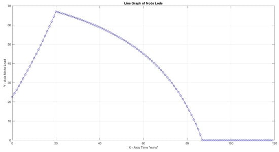
Figure 8.
Highest load for , 30 .
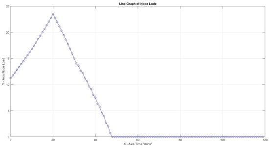
Figure 9.
Highest load for , 30 .
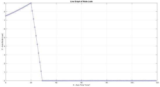
Figure 10.
Highest load for , 30 .
For the current test, it is assumed that no cognitive switching applies and that a time frame of 120 min will be set. In addition, the load control is not activated in the current context, and the slow start mechanism has not been initiated.
The results are illustrated below (Table 4):
Table 4.
Node load for CF variations.
In the first three cases, the effect of the Capacity Factor on the node load for 30 tasks with task weights assigned as can be seen. Turnaround load is not considered for the whole time framework but only for the period of active capacity activity. The highest node load for is limited to 9% compared to 67% for . This is an expected result since increased CF provides better task utilization. In all three cases, node efficiency is 100%.
In Figure 8, with CF = 1, the maximum slope peaks at 2.64, which is notably higher than 0.72 at CF = 2 and 0.08 at CF = 3. All peaks were observed early at x = 21, indicating a non-gradual transition towards high load. In addition, this observation indicates that a higher CF value allows for more efficient handling of the workload, making it more manageable.
In the following scenarios, we vary the CF but also introduce the productivity loss factor, as stated by Rubinstein et al. [41].
In all four scenarios above, variation of productivity loss due to cognitive shift can lead to a high node load to accomplish all tasks in the predefined time frame of 120 s for . It is remarkable that for productivity loss of 40% and CF = 1, the load reaches loadability early on: reaching almost infinity after 120 min. The maximum slopes for Figure 11, Figure 12, Figure 13 and Figure 14 are 0.41, 0.94, and 3.64, respectively, and it is up to x = 21 min and 1250.00 for the last scenario, which reaches infinity. What can be deduced from the values above is that, again, the load is reaching high values early on in most cases, and a low Capacity Factor with high productivity loss due to cognitive switching causes the opposite results of what would happen if there was a smooth flow in the workload (Table 5).
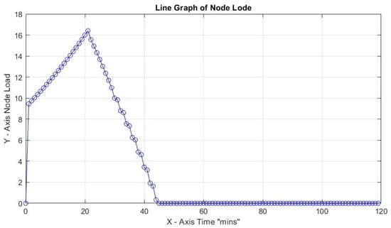
Figure 11.
Highest load 16% for CF = 3, 30 , and productivity loss 20%.
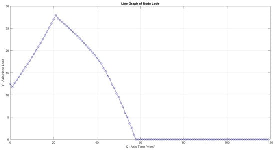
Figure 12.
Highest load 27% for CF = 3, 30 , and productivity loss 40%.
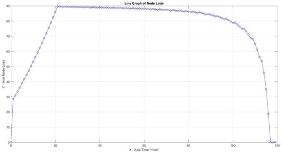
Figure 13.
Highest load 89% for CF = 1, 30 , and productivity loss 20%.
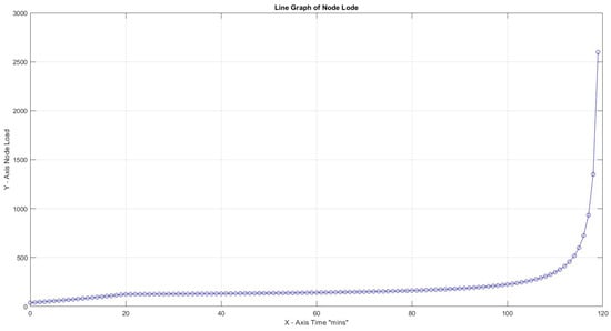
Figure 14.
Highest load 2600% for CF = 3, 30 , and productivity loss 40%.
Table 5.
Node load on CF variations, productivity loss due to cognitive switching added.
In the next two scenarios, we provide an initial 10 tasks, and as the receiving node starts processing, an additional set of 30 tasks is added, thus increasing the total number of tasks by 10 compared to previous tests. All tasks are sent serially and each one with higher priority, thus forcing Node B to switch with every received job.
So for the two scenarios above, we deploy 40 tasks over the same period of 120 min. Production loss is set to a minimum of 20%. In Figure 15, it is impressive that the node reaches loadability early (after 20 s of traffic initiation), while no task has been completed. Since the load keeps increasing, it means that up to the end of the time frame, no human can finish any task in actual circumstances. In the following scenario, as illustrated in Figure 16, the results are remarkable when load control is applied to loadability, with rejection of any task above this threshold. Only 11 out of 40 tasks were rejected, and the plot shows stable loadability behavior (Table 6).
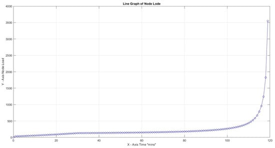
Figure 15.
CF = 1, productivity loss 20%, 40 , and no load control.

Figure 16.
CF = 1, productivity loss 20%, 40 , and load control.
Table 6.
Node load on CF variations.
The last experiment was conducted using a slow start. The results showed a smoother transition towards loadability. Due to rejections, the exact same number of tasks was completed as in scenario 15, but, most importantly, most tasks resided on the source node. In case of failure of Node B, the remaining functions are not deadlocked but remain with a pending status on the sending node, providing flexibility in traffic distribution. The maximum slope is achieved at x = 71 min, which is quite later than previous values (x = 21), indicating a gradual transition to loadability. Load drops are considered normal behavior since no additional task can interfere if the history (window size) prevents more tasks from being sent toward Node B (Table 7).
Table 7.
Node load on Slow Start activated.
As far as efficiency of the nodes is concerned, we observe that when no load control is activated, no task can be completed in realistic time measurements (no excess of loadability); therefore, it reaches almost zero. On the other hand, with load control activated, regardless of the slow start mechanism, we reach 29 completed out of 40 potentially completed tasks, which provides, according to (9) .
What is valuable to identify is how fast the node leads to loadability.
So the results show a smooth transition to loadability for the history-enabled scenario, which proves that this approach was wisely selected as the regulation driver.
- Key Findings
The primary findings of our experiment indicate a tolerance to the node load as the Capacity Factor increases, aligning with our initial expectations. Specifically, certain combinations of factors result in proportional employee capability, as demonstrated in Figure 8 and Figure 9. Cognitive switching impacts the quantity of tasks each node re-processes, which can cause delays and necessitate increased effort. This process may even lead to a “blackout” within a given time frame, as illustrated in Figure 11 through Figure 14. Introducing a load control mechanism, which ensures tasks are assigned to employees only when necessary, effectively prevents scenarios leading to dead ends, as shown in Figure 15 and Figure 16. The pinnacle of our research is represented by the integration of the slow start algorithm. This algorithm ensures a gradual increase in load, even during load surges, thereby avoiding overload conditions. This outcome is depicted in Figure 17.
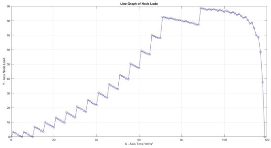
Figure 17.
CF = 1, productivity loss 20%, 40 , no load control, and slow start.
Our choice of employing root mean squared error (RMSE) and mean absolute percentage error (MAPE) for validation purposes in the context of this study, particularly in the comparison between the adaptive neuro-fuzzy inference system (ANFIS) and other methodologies like artificial neural networks (ANNs), linear regression, support vector machines (SVMs), and gradient boosting machines (GBMs) was primarily driven by the unique characteristics of the research. While the comprehensive results fall beyond this paper’s immediate scope, we provide insights into the outcomes generated from a specific configuration. Notably, the RMSE value obtained for the ANFIS was 35.83, contrasting with considerably higher RMSEs of 47.81 for an ANN with three hidden layers of 8, 4, and 4 neurons, respectively, 52.73 for linear regression, 54.21 for an SVM, and 52.29 for a GBM (Table 8). It should be acknowledged that further configurations and experiments could be explored and undertaken to corroborate the validity of our selected method.
Table 8.
Algorithm comparison.
5. Discussion
5.1. Research Achievements
Based on the research of Michalopoulos et al. [6], the proposed workload management system model is a hybrid adaptive approach that could be deployed under any circumstances in the public sector. Following the relation between skills (factors) and the Capacity Factor, an update to any skill could consequently affect the produced Capacity Factor. For factors . So the workload that each employee is theoretically handling, up to the loadability level, directly depends on those factors. Utilizing a complete dataset of skills and the corresponding capacity factors, a potential change of , for instance, would provide a CF for which the future workload could be foreseen and to which management plans would be applied.
The current study has yielded several significant findings that contribute to the understanding and implementation of a workload management system within the public sector. First and foremost, our research confirms the hypothesis that an increase in the Capacity Factor corresponds with a greater tolerance to the node load. This finding is critical as it highlights the robustness of our model under varying load conditions and validates the foundational assumptions of our approach. As depicted in Figure 8 and Figure 9, specific combinations of factors result in proportional employee capabilities, ensuring that the system can adapt to different workload scenarios effectively.
Another notable achievement is the elucidation of the impact of cognitive switching on task processing. A cognitive switch, defined as the transition between different tasks, significantly affects the quantity of tasks each node re-processes. Our results indicate that frequent cognitive switching can introduce delays and necessitate additional effort, potentially leading to a “blackout” within a specified time frame, as shown in Figure 11, Figure 12, Figure 13 and Figure 14. Without careful planning, cognitive switches become an unpredictable factor in the load balance equation. This insight underscores the need for careful planning and management of task allocation to mitigate the adverse effects of cognitive switching.
Furthermore, the introduction of a load control mechanism represents a pivotal advancement for preventing system overloads and dead-end scenarios. This mechanism ensures that tasks are assigned to employees only when necessary, thereby maintaining a balanced workload distribution and enhancing overall system efficiency. The effectiveness of this approach is illustrated in Figure 15 and Figure 16, where the implementation of load control successfully averts conditions that could lead to operational bottlenecks.
A key aspect of our research was the integration of the slow start mechanism. This algorithm facilitates a gradual increase in load, even during periods of load surges, thereby preventing overload conditions and ensuring a stable and manageable increase in workload. As depicted in Figure 17, the slow start algorithm allows for a smooth transition to higher load levels, maintaining system stability and preventing employee burnout. This gradual approach to load management is particularly beneficial in dynamic environments where workloads can fluctuate unpredictably. Additional research on the deployed slow start algorithm is out of the scope of the DWMS. In addition, retransmission issues are not applicable at this level as there is no high traffic that could justify the adoption of such a mechanism. Preanalysis results showed that the ANFIS, compared to algorithms such as an ANN, linear regression, a support vector machine, and a gradient boosting machine, showed better results in terms of RMSE (root mean squared error) and MAPE (mean absolute percentage error). Nevertheless, what is hard to predict in any system based on human attitude is the behavior of an employee on a “bad day”, which could affect the imbalance–equilibrium of the workload in the proposed system.
Investigating the impact of task switching on the overall load distribution among public body employees was particularly insightful. Task switching, if not meticulously planned, introduces a variable element in the load balance equation, making it unpredictable. Equally important in the analysis is the efficacy of the slow start deployment, which ensures a seamless transition to loadability by leveraging load control at the overload threshold. This mechanism consistently allows employees to operate at the necessary load level, avoiding both underutilization and burnout. It is worth noting that further exploration of the slow start algorithm’s deployment extends beyond the scope of the DWMS. Additionally, retransmission concerns are irrelevant in this context due to the absence of high traffic that would necessitate such measures. When comparing the ANFIS to an ANN, the ANFIS demonstrated superior performance regarding the RMSE and CF values. Nonetheless, a key challenge in any human-centric system is predicting performance fluctuations due to personal factors, which can significantly impact workload stability in the proposed system.
5.2. Limitations
Our study’s generalizability might be limited due to the sample size and chosen methodology. The data samples may not represent the entire population, potentially affecting the results’ applicability to other contexts. Additionally, while ANFIS is a valuable tool for modeling employee assessment systems, its accuracy can be impacted by limited data or unspecified variables. Future research could address these limitations by collecting data from a broader, more diverse group and exploring more advanced modeling techniques to enhance accuracy. While effective, the proposed workload management system (DWMS) has some limitations that warrant consideration. Scalability is a key concern, as the system’s performance in larger, complex public sector organizations remains untested. Future research should explore its application across various organizational sizes. Human behavior variability also poses a challenge. The current model does not fully account for performance fluctuations due to personal factors, which can impact workload balance. Integrating advanced behavioral models could enhance system accuracy. Data quality is another critical issue. The DWMS relies on accurate and complete employee data, and inaccuracies can lead to inefficiencies. Future studies should focus on improving data collection and validation processes. The slow start algorithm, while effective, needs optimization for environments with rapid workload surges. Enhancing its flexibility and adaptability is essential for broader applicability.
5.3. Practical Considerations for Implementation
Implementing the proposed workload management system (DWMS) in the public sector requires addressing several practical considerations to ensure effectiveness and sustainability. First, accurate assessment and continuous updating of employee skills is essential. Training programs should be in place to maintain up-to-date skill levels, ensuring the DWMS can allocate tasks appropriately based on current capabilities. Real-time monitoring and feedback mechanisms are crucial for maintaining system balance. These tools can quickly identify and address any imbalances or overloads, preventing inefficiencies and ensuring smooth operations. Customization and flexibility of the DWMS are also important. Public sector organizations vary widely in their workflows and employee capabilities. The system should be adaptable to meet the specific needs of different organizations, allowing for tailored workload management solutions. Furthermore, clear communication and a change to management strategies are vital for successful implementation. Employees should be informed and trained on the new system, and their feedback should be incorporated to enhance the system’s acceptance and effectiveness. Lastly, ensuring robust data security and privacy measures is critical. The DWMS relies on sensitive employee data, and protecting this information is essential for maintaining trust and compliance with regulations.
6. Conclusions and Future Work
The present research offers a robust framework for enhancing the efficiency and effectiveness of public sector organizations through a structured workload management system. This system facilitates the optimized distribution, monitoring, and adjustment of employee work assignments, leading to the efficient utilization of resources and enhanced employee productivity. By aligning workloads with employee capabilities and capacities, the system ensures a balanced distribution of tasks, thereby mitigating the risks of burnout and stress-related issues. Moreover, this approach enhances project planning and resource allocation, resulting in timely project completion and increased client satisfaction. Overall, the implementation of a well-designed workload management system promotes a healthier work environment, fosters employee engagement, and supports the organization in achieving its strategic goals effectively and sustainably. Future research should aim to extend the applicability and scalability of the proposed workload management system (DWMS) across diverse public sector environments. This involves conducting pilot studies in various organizational settings to evaluate the system’s performance and adaptability. Additionally, integrating advanced technologies such as artificial intelligence (AI) and machine learning (ML) can further enhance the system’s predictive capabilities and responsiveness. One of the significant future directions is the development of a holistic node clustering strategy within a dynamic workload management system. This approach can dynamically group nodes based on real-time workload demands and employee skill sets, allowing for more efficient task allocation and load balancing. Implementing such a system can reduce the impact of node failures by redistributing tasks to other capable nodes swiftly, thereby maintaining operational continuity and minimizing disruptions. Another promising area for future research is the exploration of virtual nodes and distributed task allocation mechanisms. In this context, virtual nodes refer to non-geographically bound nodes that can handle tasks remotely. By leveraging cloud computing and virtualization technologies, public sector organizations can manage workloads through distributed networks of virtual nodes. This approach not only enhances flexibility and scalability but also allows for the efficient handling of workload spikes and unforeseen disruptions. Incorporating sophisticated human behavioral models into the DWMS is crucial for addressing the variability in employee performance due to personal factors. These models can predict and manage fluctuations in individual performance, thereby improving workload distribution accuracy. Future studies should focus on developing and integrating these behavioral models to enhance the system’s overall reliability and effectiveness. Ensuring high-quality data is paramount for the DWMS to function effectively. Future research should prioritize the development of robust data collection and validation methods to guarantee accurate and complete employee data input. Additionally, maintaining data security and privacy is essential, especially when dealing with sensitive employee information. Implementing advanced encryption and access control measures can protect data integrity and maintain trust. The slow start algorithm, while effective at managing gradual load increases, requires further optimization for environments characterized by rapid workload surges. Enhancing the algorithm’s flexibility and adaptability can improve its performance under varying load conditions. Future research should explore modifications and improvements to the slow start algorithm to ensure its applicability in diverse operational settings. Conducting comparative analyses with other workload management models can identify best practices and integrate effective elements from various approaches. Such comparative studies will strengthen the DWMS and contribute to more efficient public sector workload management. Future research should aim to benchmark the DWMS against alternative models to highlight its advantages and areas for improvement. In conclusion, the proposed workload management system has the potential to revolutionize the way public sector organizations manage their workforces. By addressing the outlined future research directions, the system can be refined and enhanced to meet the evolving needs of public sector entities, ultimately leading to improved operational efficiency and employee satisfaction. This marks the beginning of a new era in employee management characterized by intelligent, adaptive, and scalable workload management solutions.
Author Contributions
K.C.G., D.M., G.V., D.P., I.G. and S.S. conceived of the idea, designed and performed the experiments, analyzed the results, drafted the initial manuscript, and revised the final manuscript. All authors have read and agreed to the published version of the manuscript.
Funding
This research received no external funding.
Data Availability Statement
The data presented in this study are available on request from the corresponding author.
Acknowledgments
We are indebted to the anonymous reviewers, whose comments helped us to improve the presentation.
Conflicts of Interest
The authors declare no conflicts of interest.
References
- Liang, L.; Kuusisto, A.; Kuusisto, J. Building strategic agility through user-driven innovation: The case of the Finnish public service sector. Theor. Issues Ergon. Sci. 2018, 19, 74–100. [Google Scholar] [CrossRef]
- Pedraja-Chaparro, F.; Salinas-Jiménez, J.; Smith, P.C. Assessing public sector efficiency: Issues and methodologies. SSRN Electron. J. 2005, 3, 343–359. [Google Scholar] [CrossRef]
- Curristine, T.; Lonti, Z.; Joumard, I. Improving public sector efficiency: Challenges and opportunities. OECD J. Budg. 2007, 7, 1–41. [Google Scholar] [CrossRef]
- Haq, F.I.U.; Alam, A.; Mulk, S.S.U.; Rafiq, F. The effect of stress and work overload on employee’s performance: A case study of public sector Universities of Khyber Pakhtunkhwa. Eur. J. Bus. Manag. Res. 2020, 5. [Google Scholar] [CrossRef]
- Huang, Q.; Wang, Y.; Yuan, K.; Liu, H. How role overload affects physical and psychological health of low-ranking government employees at different ages: The mediating role of burnout. Saf. Health Work. 2022, 13, 207–212. [Google Scholar] [CrossRef] [PubMed]
- Michalopoulos, D.; Karras, A.; Karras, C.; Sioutas, S.; Giotopoulos, K. Neuro-Fuzzy Employee Ranking System in the Public Sector. In Fuzzy Systems and Data Mining VIII; IOS Press: Amsterdam, The Netherlands, 2022; Volume 358, p. 325. [Google Scholar]
- Giotopoulos, K.C.; Michalopoulos, D.; Karras, A.; Karras, C.; Sioutas, S. Modelling and analysis of neuro fuzzy employee ranking system in the public sector. Algorithms 2023, 16, 151. [Google Scholar] [CrossRef]
- Theodorakopoulos, L.; Antonopoulou, H.; Mamalougou, V.; Giotopoulos, K. The drivers of volume volatility: A big data analysis based on economic uncertainty measures for the Greek banking system. SSRN Electron. J. 2022. [Google Scholar] [CrossRef]
- Theodorakopoulos, L.; Halkiopoulos, C.; Papadopoulos, D. Applying Big Data Technologies in Tourism Industry: A Conceptual Analysis. In Proceedings of the International Conference of the International Association of Cultural and Digital Tourism, Syros Island, Greece, 1–3 September 2022; pp. 337–352. [Google Scholar]
- Adams, A.C.; Muir, S.; Hoque, Z. Measurement of sustainability performance in the public sector. Sustain. Account. Manag. Policy J. 2014, 5, 46–67. [Google Scholar]
- Boj, J.J.; Rodriguez-Rodriguez, R.; Alfaro-Saiz, J.J. An ANP-multi-criteria-based methodology to link intangible assets and organizational performance in a Balanced Scorecard context. Decis. Support Syst. 2014, 68, 98–110. [Google Scholar] [CrossRef]
- Propper, C.; Wilson, D. The use and usefulness of performance measures in the public sector. Oxf. Rev. Econ. Policy 2003, 19, 250–267. [Google Scholar] [CrossRef]
- Arnaboldi, M.; Lapsley, I.; Steccolini, I. Performance management in the public sector: The ultimate challenge. Financ. Account. Manag. 2015, 31, 1–22. [Google Scholar] [CrossRef]
- Gunarsih, T.; Saleh, C.; Nur Syukron, D.; Deros, B.M. A hybrid balanced scorecard and system dynamics for measuring public sector performance. J. Eng. Sci. Technol. 2016, 11, 65–86. [Google Scholar]
- Bruhn, A.; Ekström, M. Towards a multi-level approach on frontline interactions in the public sector: Institutional transformations and the dynamics of real-time interactions. Soc. Policy Adm. 2017, 51, 195–215. [Google Scholar] [CrossRef]
- Afonso, A.; Schuknecht, L.; Tanzi, V. Public sector efficiency: An international comparison. Public Choice 2005, 123, 321–347. [Google Scholar] [CrossRef]
- Goudswaard, A.; Dhondt, S.; Vergeer, R.; Oeij, P.; de Leede, J.; van Adrichem, K.; Csizmadia, P.; Makó, C.; Illéssy, M.; Tóth, Á.; et al. Organisation of Working Time: Implications for Productivity and Working Conditions—Overview Report; Eurofound: Dublin, Ireland, 2013. [Google Scholar]
- Diamond, J. 9 Measuring Efficiency in Government: Techniques and Experience. In Government Financial Management; International Monetary Fund: Washington, DC, USA, 1990; pp. 142–166. [Google Scholar]
- Kotler, P.; Lee, N. Social Marketing: Influencing Behaviors for Good; Sage Publications: Los Angeles, CA, USA, 2008. [Google Scholar]
- Collewet, M.; Sauermann, J. Working hours and productivity. Labour Econ. 2017, 47, 96–106. [Google Scholar] [CrossRef]
- Pencavel, J. The productivity of working hours. Econ. J. 2015, 125, 2052–2076. [Google Scholar] [CrossRef]
- Dolton, P.; Howorth, C.; Abouaziza, M. The optimal length of the working day: Evidence from Hawthorne experiments. In Proceedings of the ESPE Conference Paper, Paris, France, 10–12 September 2016. [Google Scholar]
- Man, N.C.; Ling, T.W. Relationships between working hours and productivity: The case of food services and information communication industries in Hong Kong. Adv. Econ. Bus. 2014, 2, 281–292. [Google Scholar] [CrossRef]
- Golden, L. The effects of working time on productivity and firm performance, research synthesis paper. In International Labor Organization (ILO) Conditions of Work and Employment Series; International Labour Office: Geneva, Switzerland, 2012. [Google Scholar]
- Bappy, M.; Musa, M.; Hossain, M. Productivity improvement through Line Balancing—A case study in an Apparel Industry. GSJ 2019, 7, 893–902. [Google Scholar]
- Di Meglio, G.; Stare, M.; Maroto, A.; Rubalcaba, L. Public services performance: An extended framework and empirical assessment across the enlarged EU. Environ. Plan. Gov. Policy 2015, 33, 321–341. [Google Scholar] [CrossRef]
- Pallathadka, H.; Wenda, A.; Ramirez-Asís, E.; Asís-López, M.; Flores-Albornoz, J.; Phasinam, K. Classification and prediction of student performance data using various machine learning algorithms. Mater. Today Proc. 2023, 80, 3782–3785. [Google Scholar] [CrossRef]
- Chowdhury, S.; Dey, P.; Joel-Edgar, S.; Bhattacharya, S.; Rodriguez-Espindola, O.; Abadie, A.; Truong, L. Unlocking the value of artificial intelligence in human resource management through AI capability framework. Hum. Resour. Manag. Rev. 2023, 33, 100899. [Google Scholar] [CrossRef]
- Prem, P.S. Machine learning in employee performance evaluation: A HRM perspective. Int. J. Sci. Res. Arch. 2024, 11, 1573–1585. [Google Scholar] [CrossRef]
- Alsheref, F.K.; Fattoh, I.E.; Ead, W.M. Automated prediction of employee attrition using ensemble model based on machine learning algorithms. Comput. Intell. Neurosci. 2022, 2022, 7728668. [Google Scholar] [CrossRef] [PubMed]
- Arslankaya, S. Comparison of performances of fuzzy logic and adaptive neuro-fuzzy inference system (ANFIS) for estimating employee labor loss. J. Eng. Res. 2023, 11, 469–477. [Google Scholar] [CrossRef]
- Achchab, S.; Temsamani, Y.K. Use of artificial intelligence in human resource management: “Application of machine learning algorithms to an intelligent recruitment system”. In Proceedings of the Advances in Deep Learning, Artificial Intelligence and Robotics: Proceedings of the 2nd International Conference on Deep Learning, Artificial Intelligence and Robotics, (ICDLAIR), Salerno, Italy, 7–18 December 2020; pp. 203–215. [Google Scholar]
- Huang, X.; Yang, F.; Zheng, J.; Feng, C.; Zhang, L. Personalized human resource management via HR analytics and artificial intelligence: Theory and implications. Asia Pac. Manag. Rev. 2023, 28, 598–610. [Google Scholar] [CrossRef]
- Tian, X.; Pavur, R.; Han, H.; Zhang, L. A machine learning-based human resources recruitment system for business process management: Using LSA, BERT and SVM. Bus. Process. Manag. J. 2023, 29, 202–222. [Google Scholar] [CrossRef]
- Casner, S.M.; Gore, B.F. Measuring and evaluating workload: A primer. NASA Tech. Memo. 2010, 216395, 2010. [Google Scholar]
- Sharifian, S.; Motamedi, S.A.; Akbari, M.K. A predictive and probabilistic load-balancing algorithm for cluster-based web servers. Appl. Soft Comput. 2011, 11, 970–981. [Google Scholar] [CrossRef]
- Xu, Z.; Wang, X. A modified round-robin load-balancing algorithm for cluster-based web servers. In Proceedings of the 33rd Chinese Control Conference, Nanjing, China, 28–30 July 2014; pp. 3580–3584. [Google Scholar]
- Diao, Y.; Shwartz, L. Building automated data driven systems for IT service management. J. Netw. Syst. Manag. 2017, 25, 848–883. [Google Scholar] [CrossRef]
- Razzaghzadeh, S.; Navin, A.H.; Rahmani, A.M.; Hosseinzadeh, M. Probabilistic modeling to achieve load balancing in expert clouds. Ad Hoc Netw. 2017, 59, 12–23. [Google Scholar] [CrossRef]
- Bellur, S.; Nowak, K.L.; Hull, K.S. Make it our time: In class multitaskers have lower academic performance. Comput. Hum. Behav. 2015, 53, 63–70. [Google Scholar] [CrossRef]
- Rubinstein, J.S.; Meyer, D.E.; Evans, J.E. Executive control of cognitive processes in task switching. J. Exp. Psychol. Hum. Percept. Perform. 2001, 27, 763. [Google Scholar] [CrossRef] [PubMed]
- Reynolds, J.R.; Donaldson, D.I.; Wagner, A.D.; Braver, T.S. Item-and task-level processes in the left inferior prefrontal cortex: Positive and negative correlates of encoding. Neuroimage 2004, 21, 1472–1483. [Google Scholar] [CrossRef] [PubMed]
- Meier, B.; Rey-Mermet, A. Beyond feature binding: Interference from episodic context binding creates the bivalency effect in task-switching. Front. Psychol. 2012, 3, 386. [Google Scholar] [CrossRef] [PubMed]
- Muhmenthaler, M.C.; Meier, B. Different impact of task switching and response-category conflict on subsequent memory. Psychol. Res. 2021, 85, 679–696. [Google Scholar] [CrossRef] [PubMed]
- Mark, G.; Gudith, D.; Klocke, U. The cost of interrupted work: More speed and stress. In Proceedings of the SIGCHI Conference on Human Factors in Computing Systems, Florence, Italy, 5–10 April 2008; pp. 107–110. [Google Scholar]
- Corbett, M. From law to folklore: Work stress and the Yerkes-Dodson Law. J. Manag. Psychol. 2015, 30, 741–752. [Google Scholar] [CrossRef]
- Shaikh, E.; Mohiuddin, I.; Alufaisan, Y.; Nahvi, I. Apache spark: A big data processing engine. In Proceedings of the 2019 2nd IEEE Middle East and North Africa COMMunications Conference (MENACOMM), Manama, Bahrain, 19–21 November 2019; pp. 1–6. [Google Scholar]
- Kanavos, A.; Livieris, I.; Mylonas, P.; Sioutas, S.; Vonitsanos, G. Apache spark implementations for string patterns in dna sequences. In Proceedings of the GeNeDis 2018: Computational Biology and Bioinformatics; Springer: Berlin/Heidelberg, Germany, 2020; pp. 439–453. [Google Scholar]
- Shyam, R.; HB, B.G.; Kumar, S.; Poornachandran, P.; Soman, K. Apache spark a big data analytics platform for smart grid. Procedia Technol. 2015, 21, 171–178. [Google Scholar] [CrossRef]
- Kanavos, A.; Panagiotakopoulos, T.; Vonitsanos, G.; Maragoudakis, M.; Kiouvrekis, Y. Forecasting winter precipitation based on weather sensors data in apache spark. In Proceedings of the 2021 12th International Conference on Information, Intelligence, Systems & Applications (IISA), Chania Crete, Greece, 12–14 July 2021; pp. 1–6. [Google Scholar]
- Vonitsanos, G.; Kanavos, A.; Mylonas, P.; Sioutas, S. A nosql database approach for modeling heterogeneous and semi-structured information. In Proceedings of the 2018 9th International Conference on Information, Intelligence, Systems and Applications (IISA), Zakynthos, Greece, 23–25 July 2018; pp. 1–8. [Google Scholar]
- Meng, X.; Bradley, J.; Yavuz, B.; Sparks, E.; Venkataraman, S.; Liu, D.; Freeman, J.; Tsai, D.; Amde, M.; Owen, S.; et al. Mllib: Machine learning in apache spark. J. Mach. Learn. Res. 2016, 17, 1–7. [Google Scholar]
- JayaLakshmi, A.; Kishore, K.K. Performance evaluation of DNN with other machine learning techniques in a cluster using Apache Spark and MLlib. J. King Saud Univ. Comput. Inf. Sci. 2022, 34, 1311–1319. [Google Scholar] [CrossRef]
- Eng, T.C.; Hasan, S.; Shamsuddin, S.M.; Wong, N.E.; Jalil, I.E.A. Big Data Processing Model for Authorship Identification. Int. J. Adv. Soft Comput. Appl. 2017, 9, 1–22. [Google Scholar]
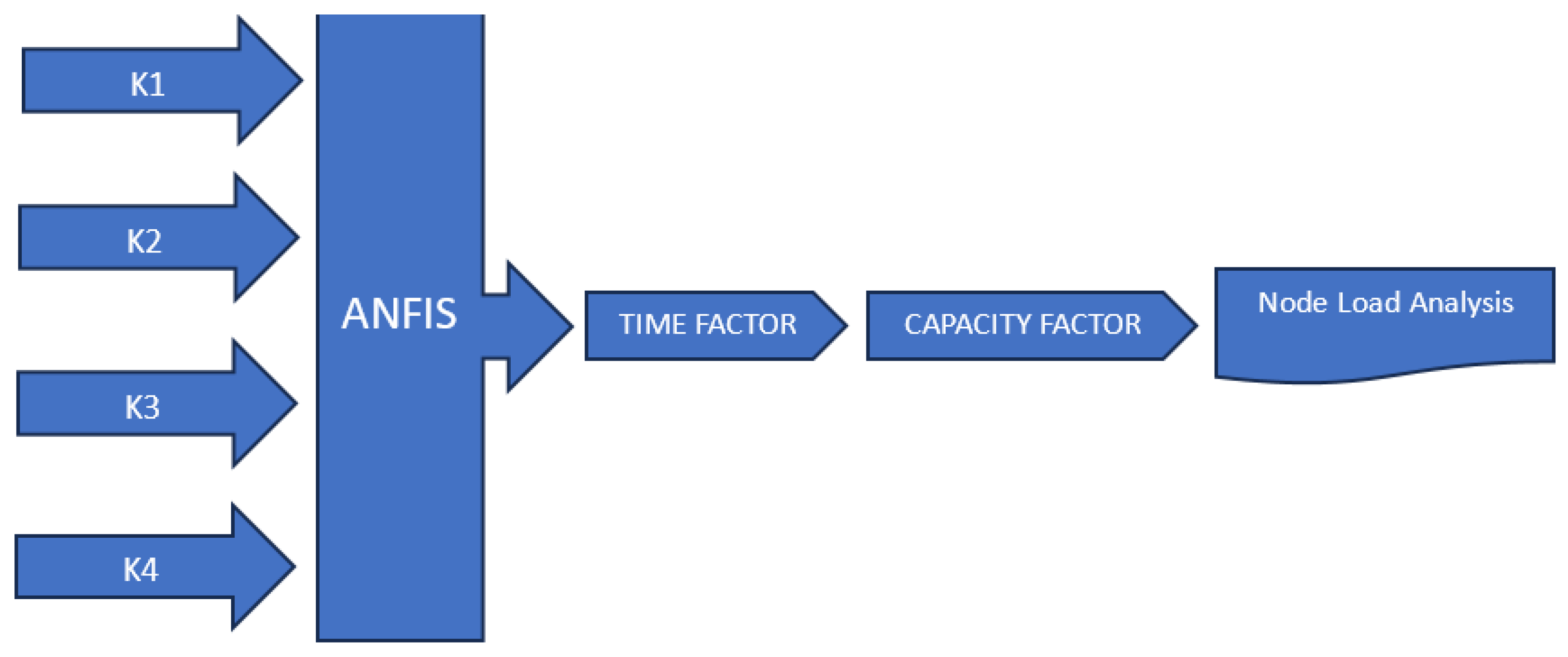
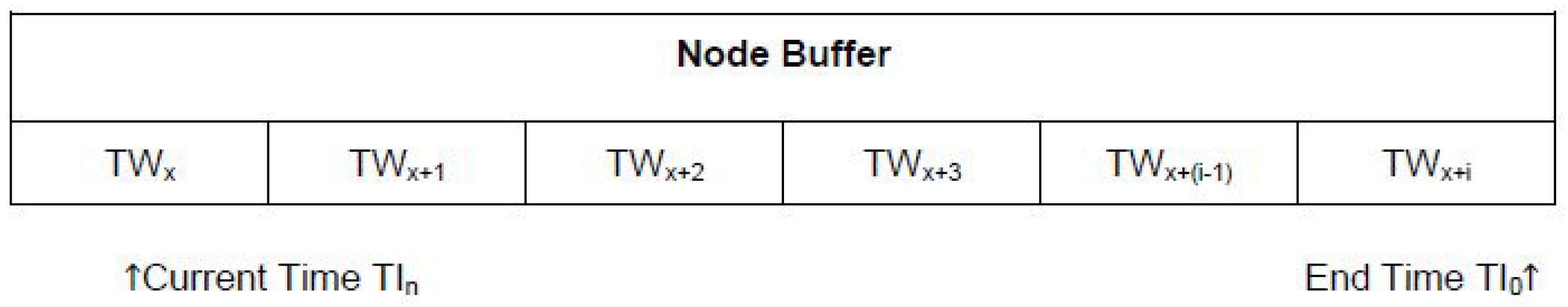
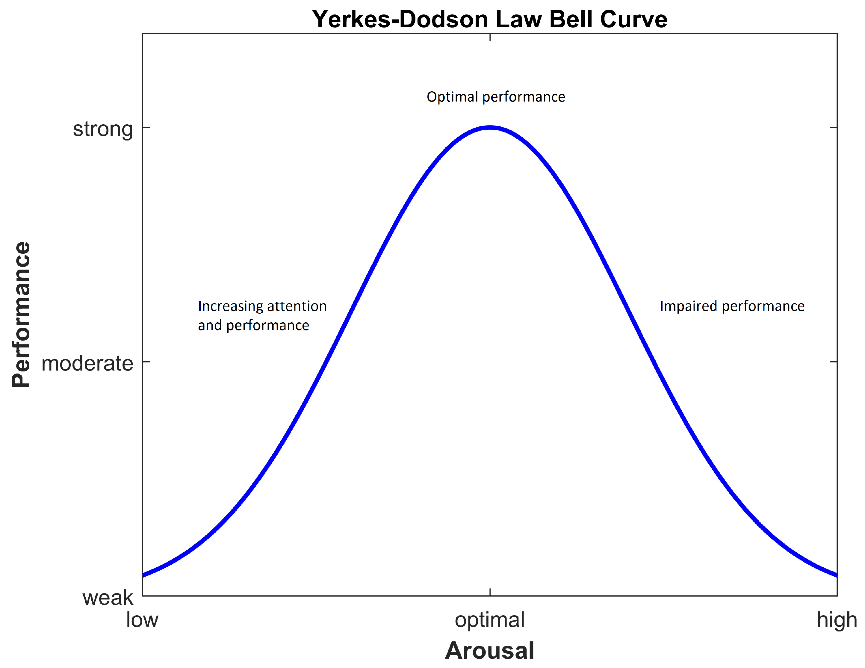
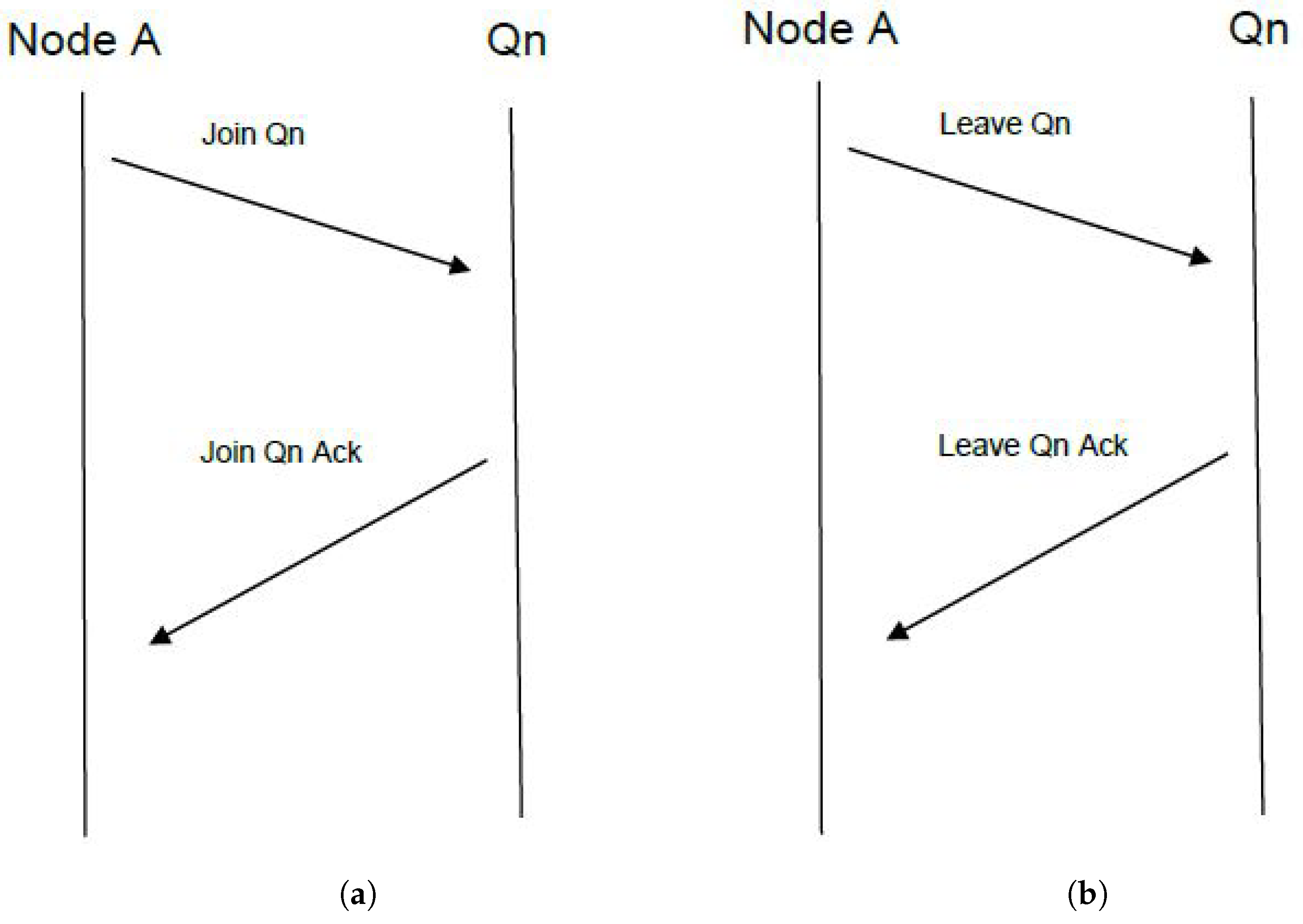
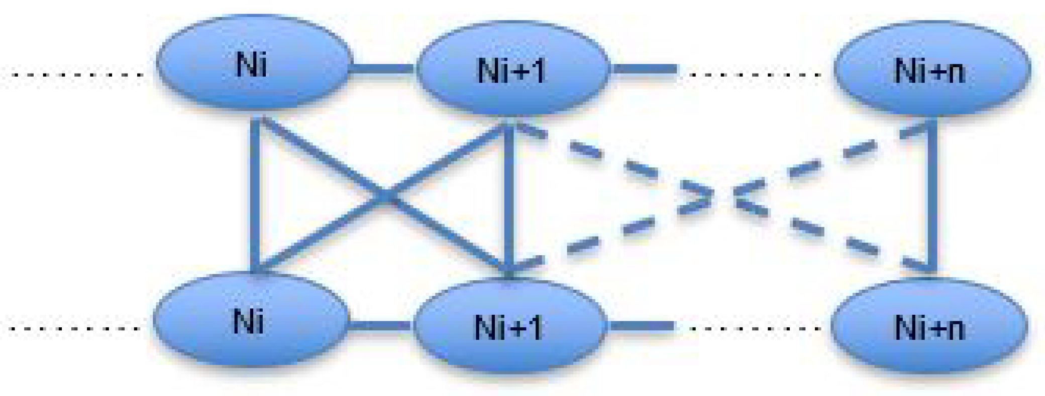
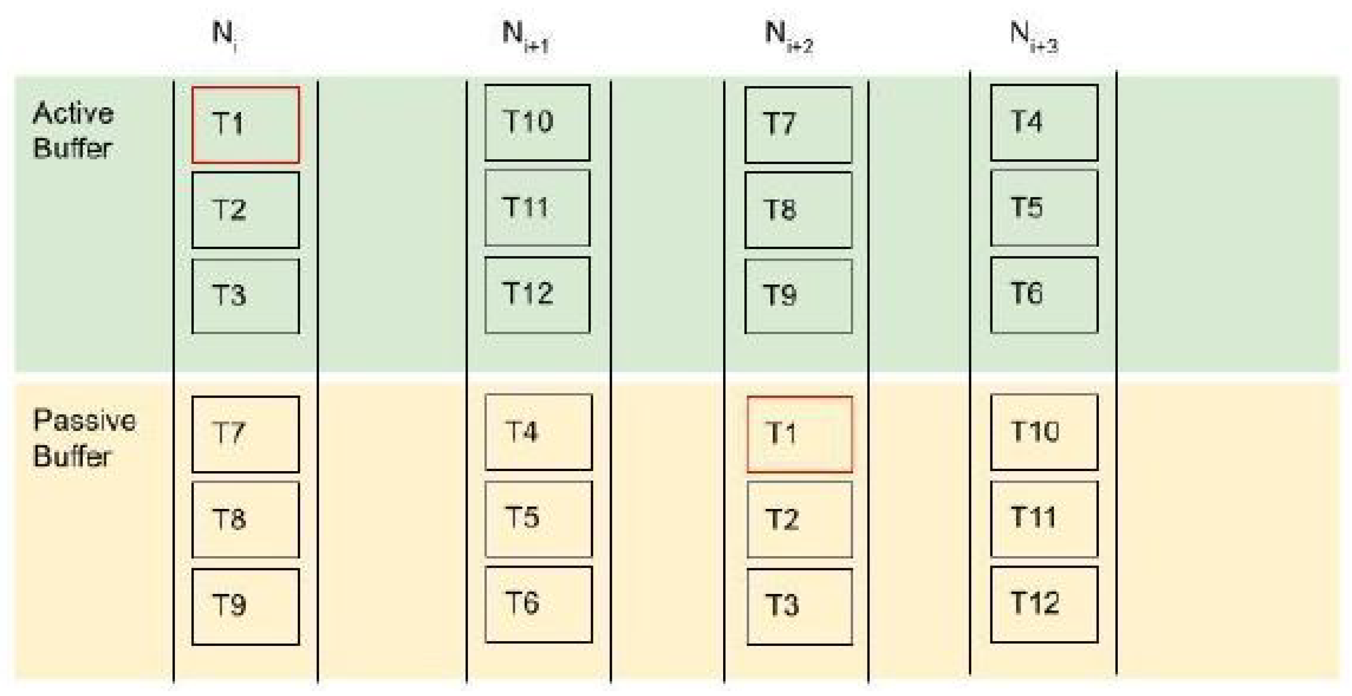
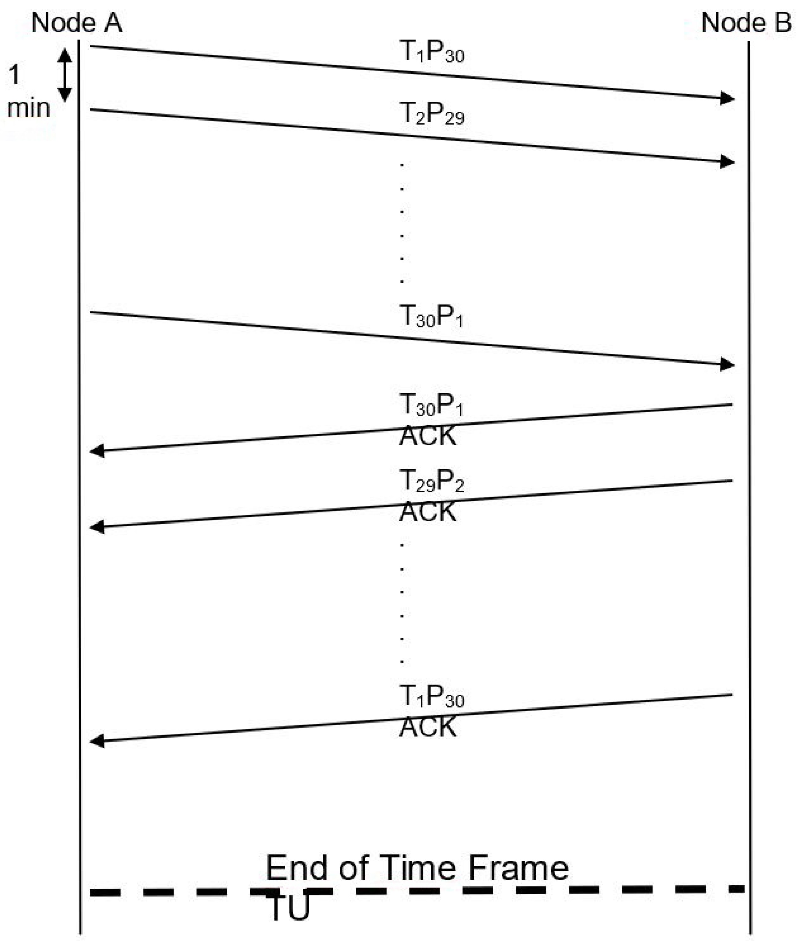
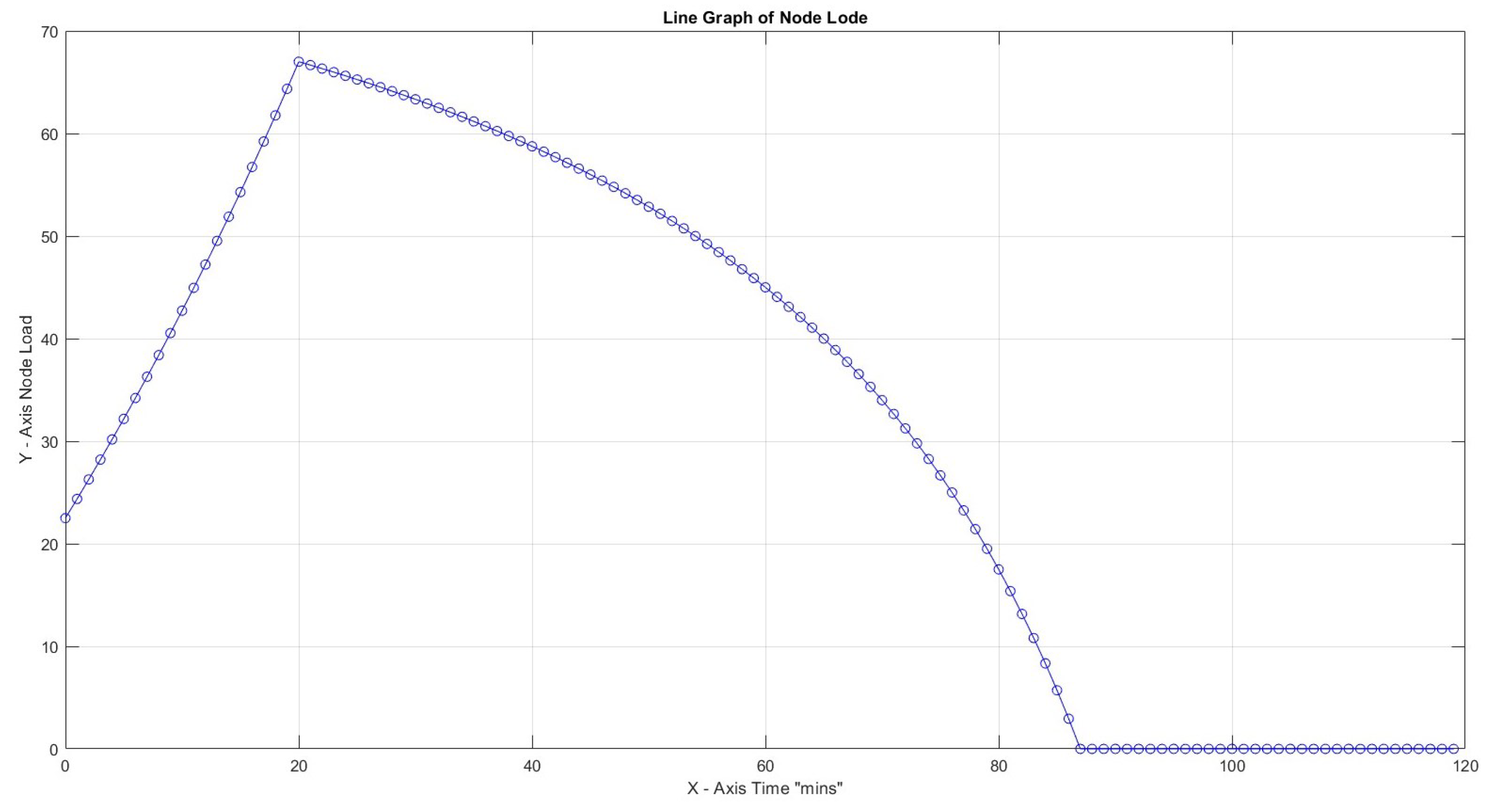
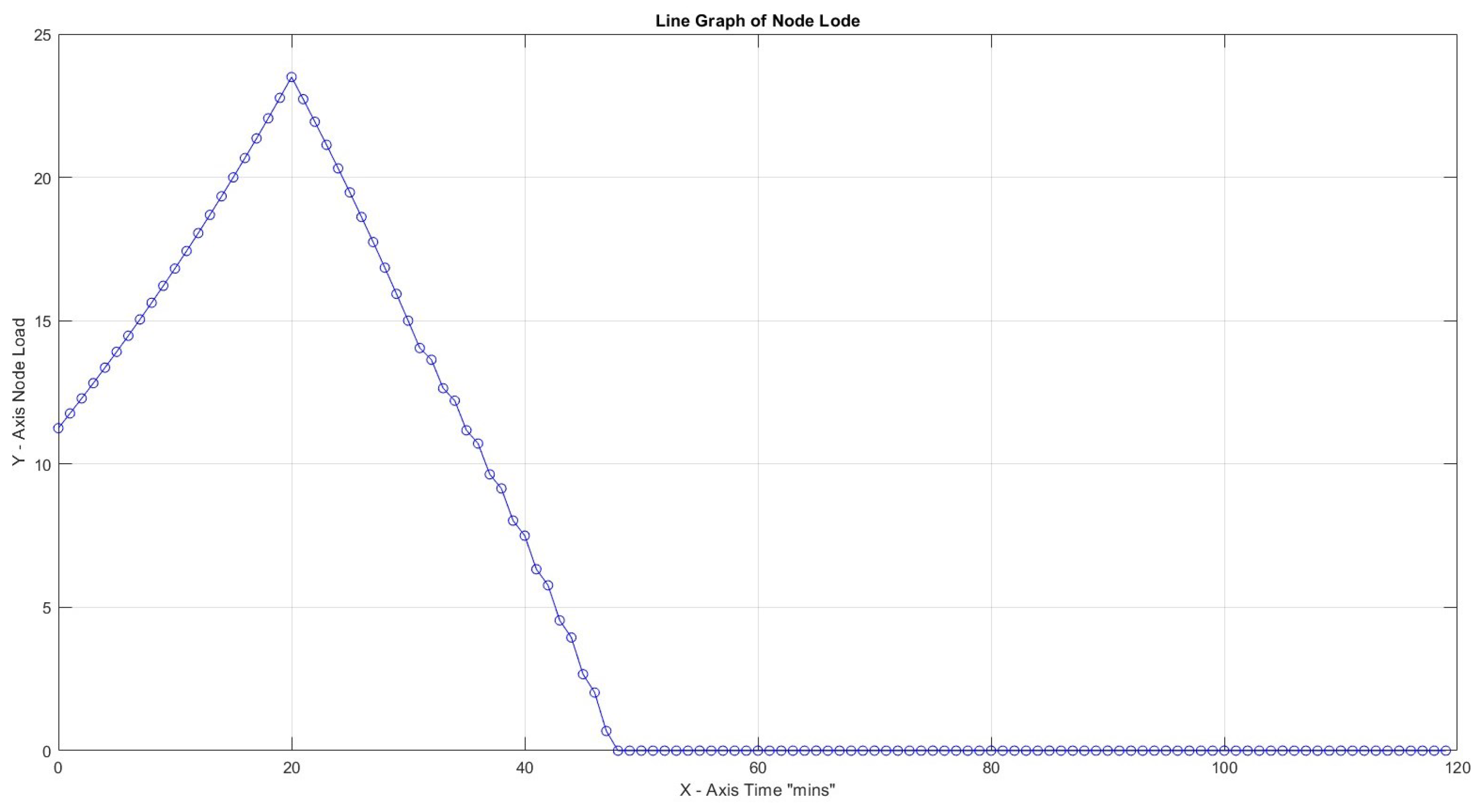
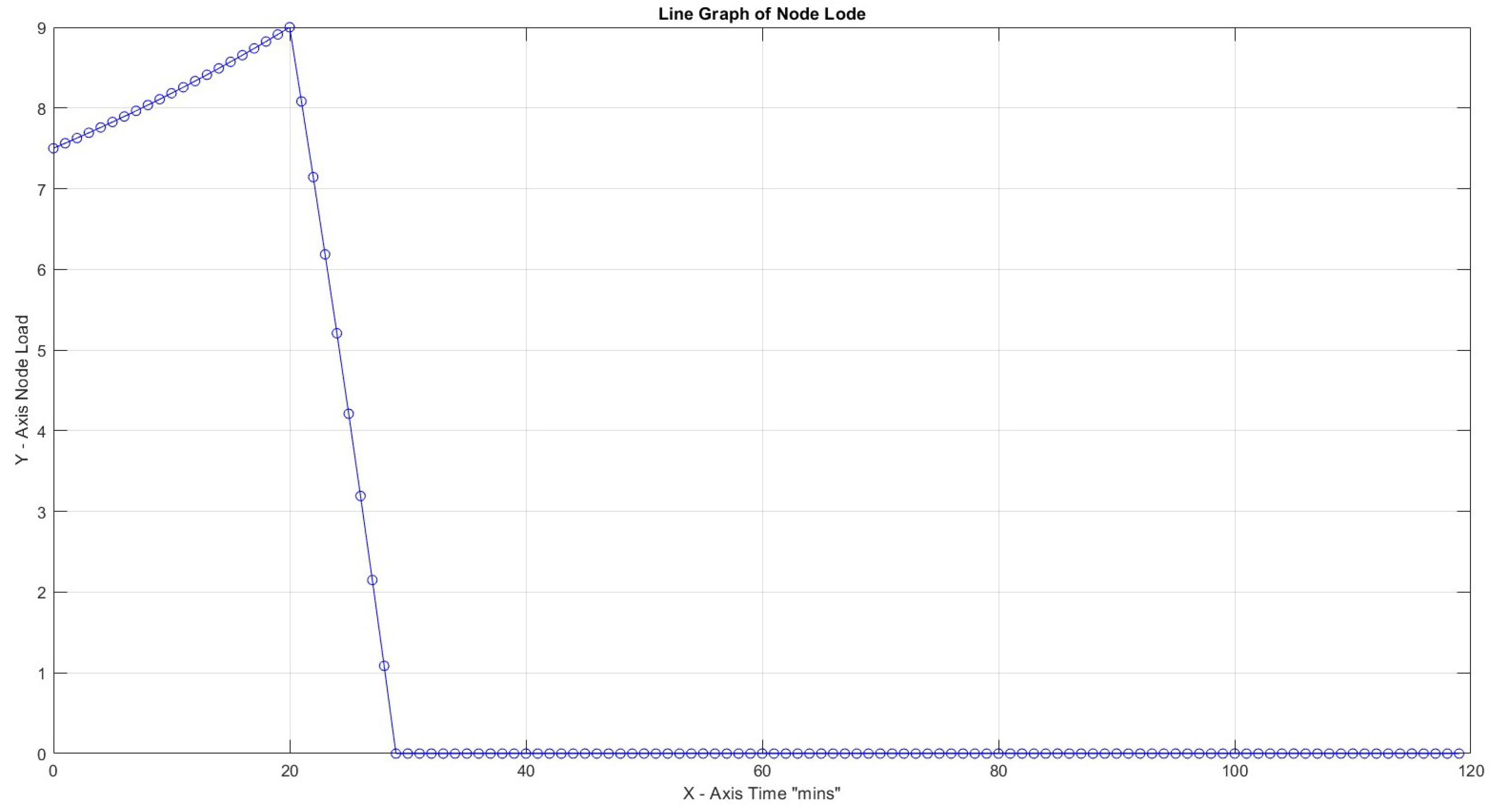
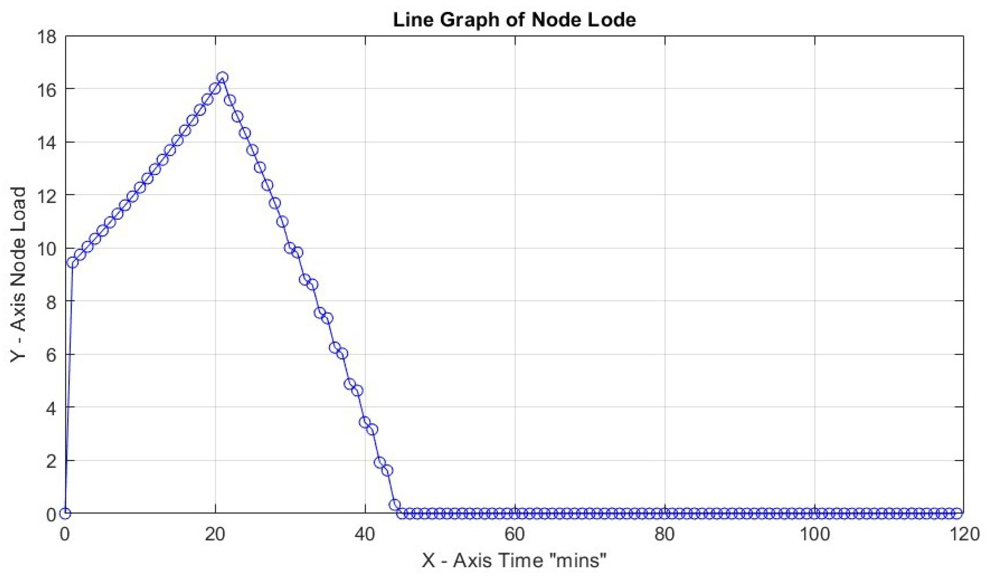
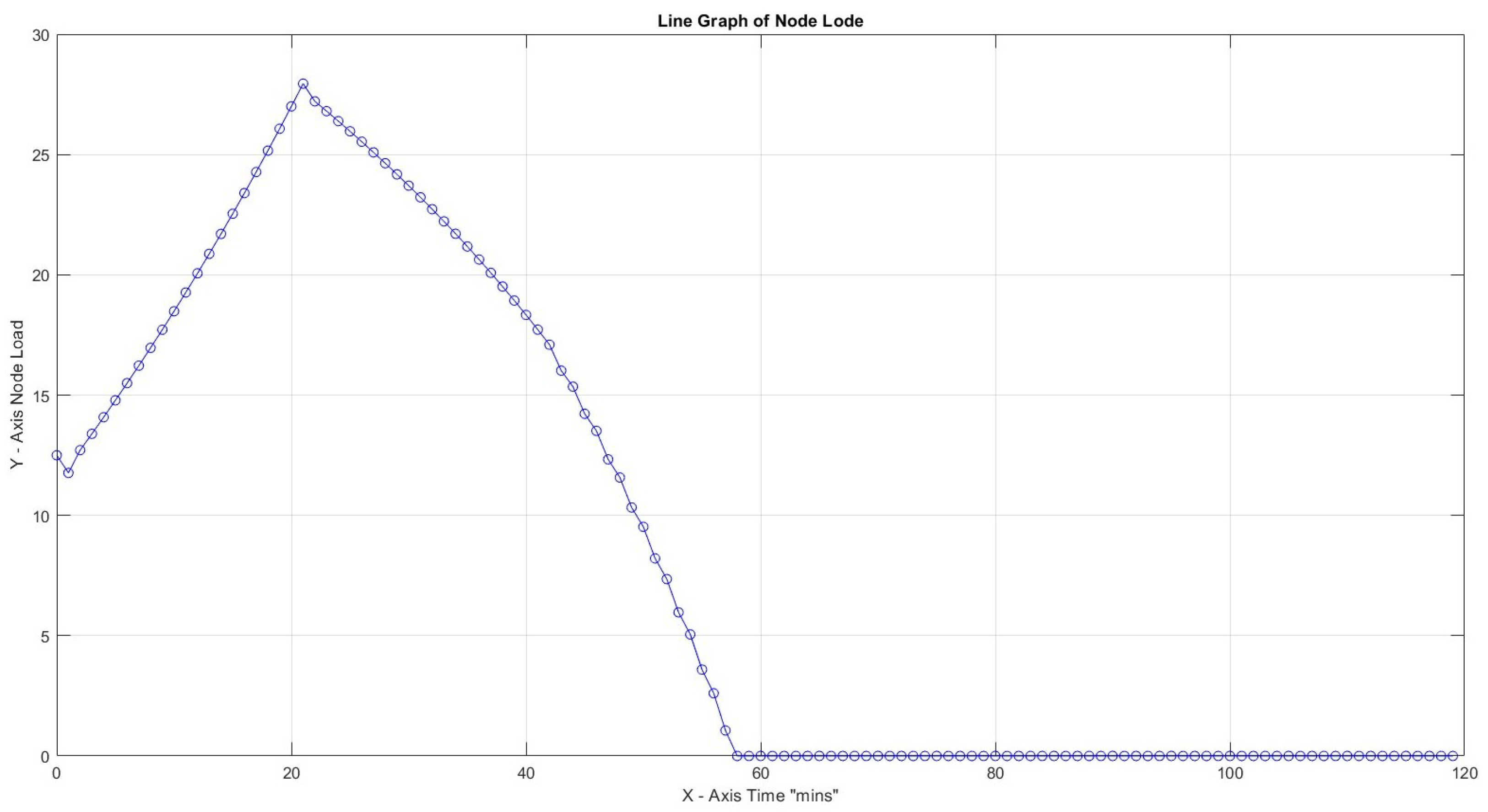
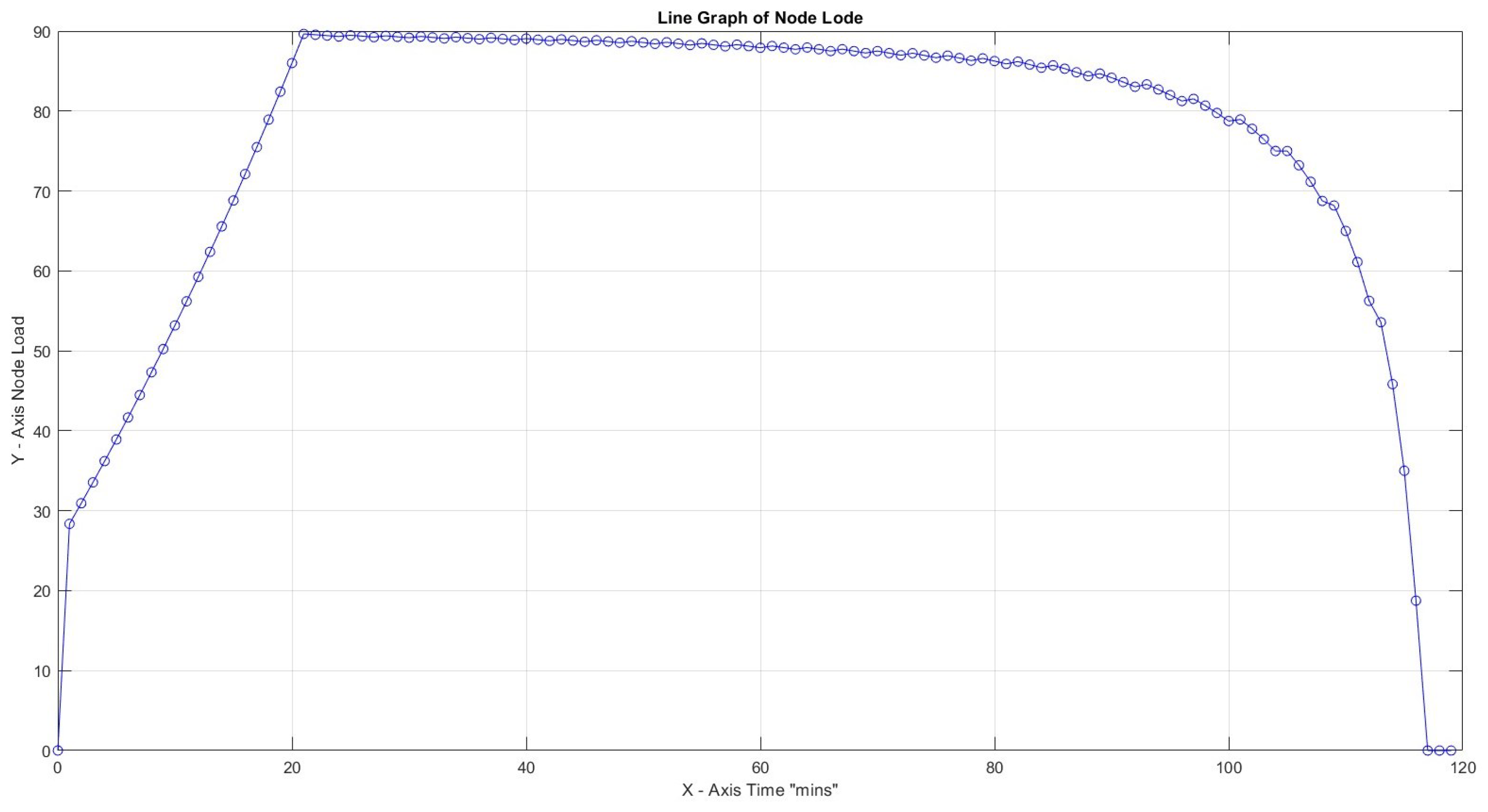
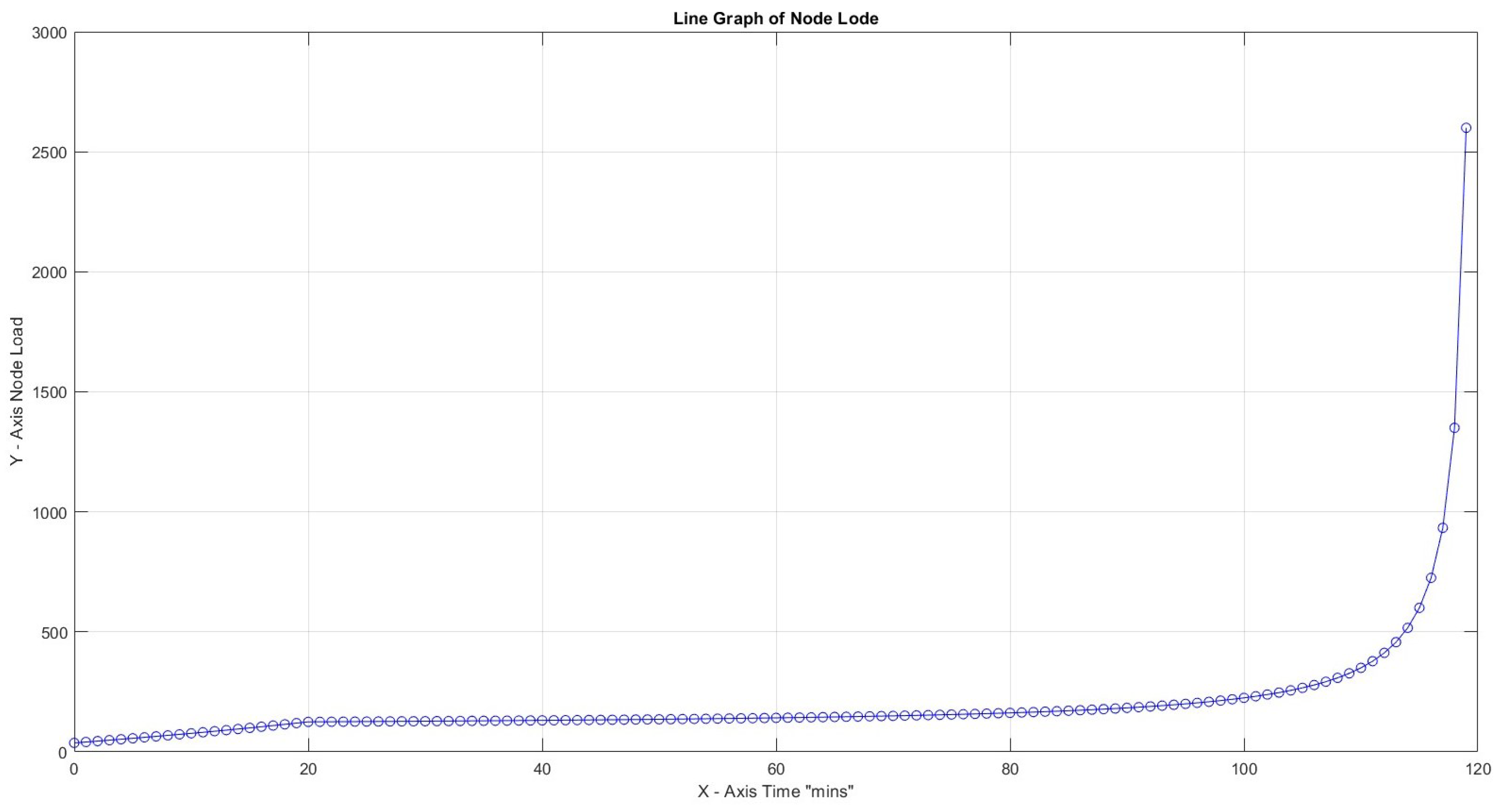
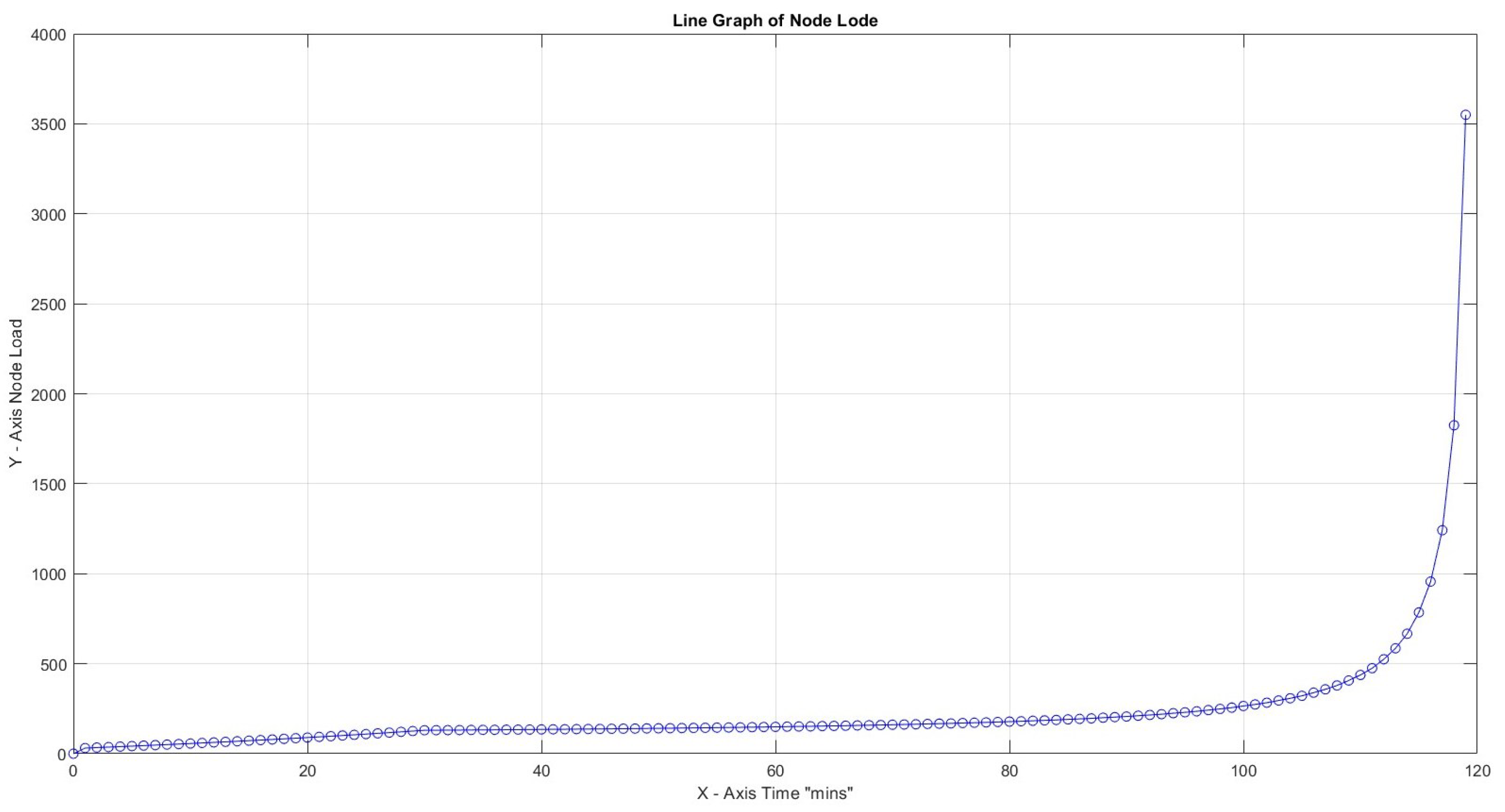
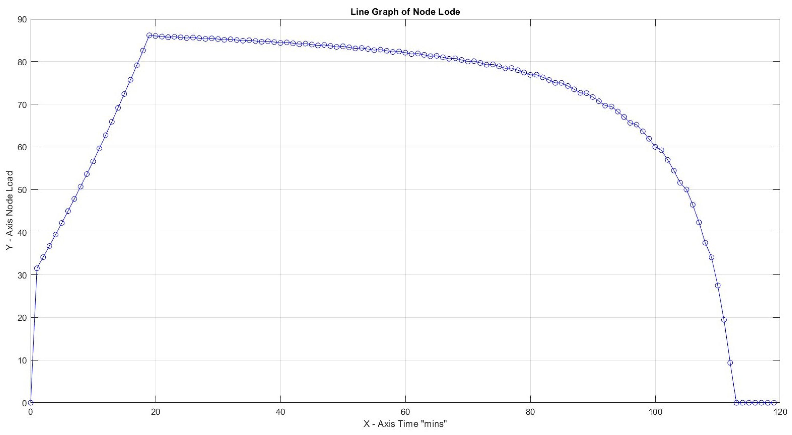
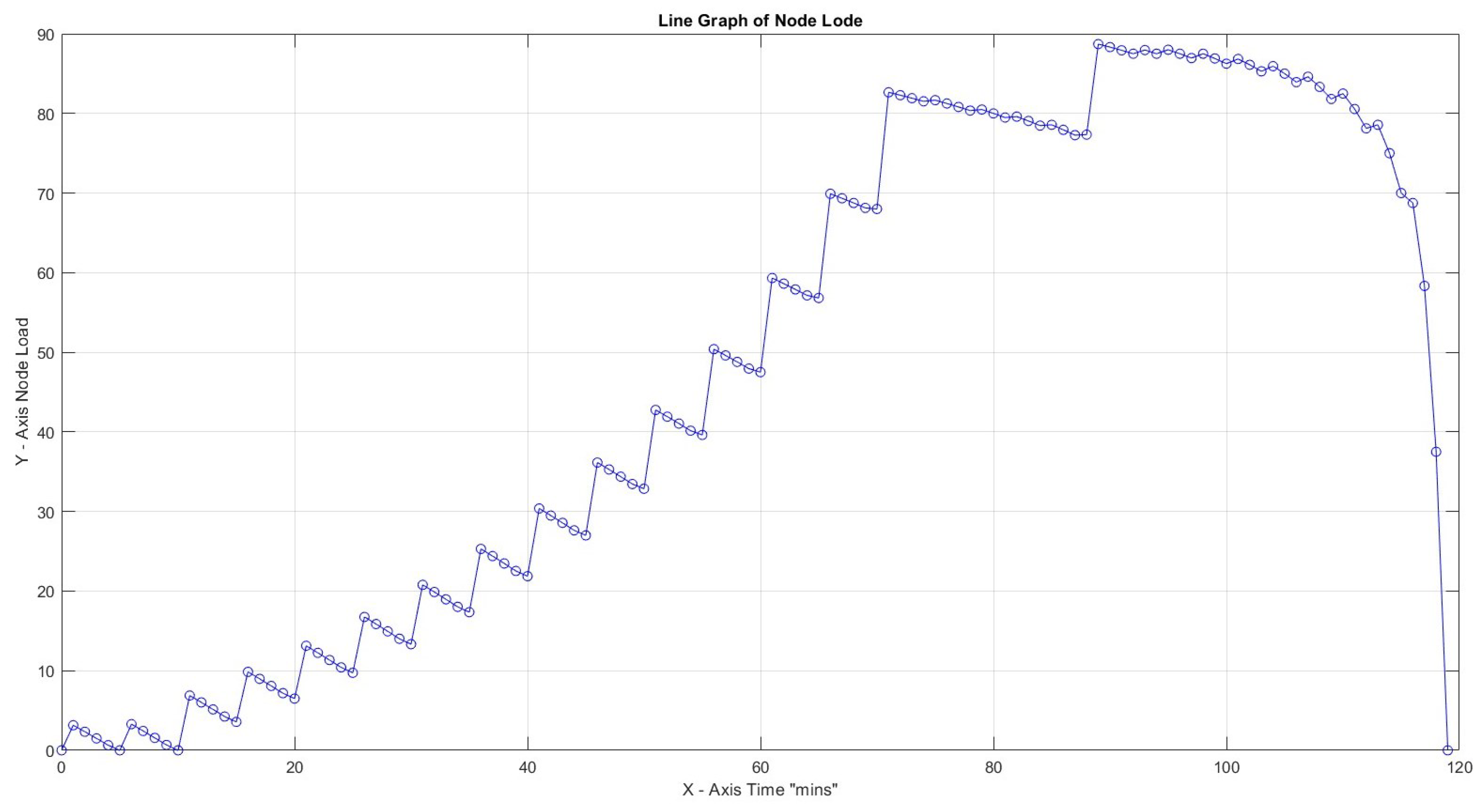
Disclaimer/Publisher’s Note: The statements, opinions and data contained in all publications are solely those of the individual author(s) and contributor(s) and not of MDPI and/or the editor(s). MDPI and/or the editor(s) disclaim responsibility for any injury to people or property resulting from any ideas, methods, instructions or products referred to in the content. |
© 2024 by the authors. Licensee MDPI, Basel, Switzerland. This article is an open access article distributed under the terms and conditions of the Creative Commons Attribution (CC BY) license (https://creativecommons.org/licenses/by/4.0/).