Two Lot-Sizing Algorithms for Minimizing Inventory Cost and Their Software Implementation

Abstract

Effective inventory management is crucial for businesses to balance minimizing holding costs while optimizing ordering strategies. Monthly or sporadic orders over time may lead to high ordering or holding costs, respectively. In this study, we introduce two novel algorithms designed to optimize ordering replenishment quantities, minimizing total replenishment, and holding costs over a planning horizon for both partially loaded and fully loaded trucks. The novelty of the first algorithm is that it extends the classical Wagner–Whitin approach by incorporating various additional cost elements, stock retention considerations, and warehouse capacity constraints, making it more suitable for real-world problems. The second algorithm presented in this study is a variation of the first algorithm, with its contribution being that it incorporates the requirement of several suppliers to receive order quantities that regard only fully loaded trucks. These two algorithms are implemented in Python, creating the software tool called “Inventory Cost Minimizing tool” (ICM). This tool takes relevant data inputs and outputs optimal order timing and quantities, minimizing total costs. This research offers practical and novel solutions for businesses seeking to streamline their inventory management processes and reduce overall expenses.

1. Introduction

Inventory management poses significant challenges due to its inherent complexity, the presence of conflicting objectives, and the influence of factors such as variability, randomness, and the rapid turnover of products. Among the critical tasks in inventory management, lot sizing stands out as one of the most important yet challenging endeavors in warehousing operations. Business executives, managers, and researchers must grapple with various factors when determining optimal replenishment strategies for their inventory.

One such factor is the planning horizon, representing the time interval into the future upon which scheduling decisions are based, which can be either finite or infinite. Additionally, the Review Interval plays a crucial role, defining the frequency at which inventory levels are reviewed and replenishment decisions are made [1]. The consideration of factors like Deterioration of Items, affecting inventory holding times, and demand variability further complicates decision-making processes. Moreover, Inventory Shortage, encompassing policies related to backorders or lost sales, adds another layer of complexity to modeling and problem-solving approaches [2].

Over the years, numerous models have been proposed and published, ranging from simplistic to more sophisticated approaches. Some “shortsighted” models advocate for ordering on a monthly or periodic basis to meet demand without considering cost reduction. Conversely, the Wagner–Whitin algorithm, optimal in terms of cost, considers only certain problem parameters. Various extensions of this algorithm have been published, each addressing specific needs of real businesses, yet none incorporates as many order characteristics as the one presented in this study.

In this study, we focus on addressing the challenges associated with variable and non-stochastic demand in inventory management. We build upon the classical Wagner–Whitin algorithm, renowned for its effectiveness in solving lot-sizing problems. The Wagner–Whitin method, introduced in 1958, is a dynamic approach that solves the economic lot-sizing problem, aiming to minimize total inventory costs over a planning horizon while considering variable production and inventory holding costs. This method computes the optimal order quantities and timings by dynamically adjusting production and inventory levels in response to changing demand patterns. By incorporating the costs associated with ordering, holding, and setup, the Wagner–Whitin algorithm enables decision-makers to strike a balance between ordering costs and holding costs, thereby optimizing inventory management processes [3].

In this study, we propose a variant of the Wagner–Whitin algorithm. The novelty of this paper resides in its integration of supplementary cost factors into the established Wagner–Whitin algorithm, rendering it applicable for implementation across diverse real-world corporate environments. This enhancement extends the algorithm’s utility beyond its conventional scope, facilitating its adoption by a broader array of companies seeking optimized, cost-effective solutions in operational decision-making processes. This contribution is vital for enhancing efficiency and cost-effectiveness in various industries, thereby fostering improved competitiveness and sustainability.

In addition, our research underscores the critical requirement within practical business logistics for the ordering of full truckloads. By elucidating the importance of this practice, our study contributes to a deeper understanding of the intricacies involved in real-world logistics operations. Moreover, our findings offer insights that can inform decision-making processes within businesses, enabling them to streamline their operations and enhance overall efficiency. This need is addressed through a second algorithm. In this manner, the demands of stakeholders for a more cost-effective ordering and inventory stocking method optimized in terms of both cost and space are met, offering them flexibility in budget and the chance to invest in other sections of the business, such as personnel or research and innovation.

Furthermore, we present the “Inventory Cost Minimizing” (ICM) software tool, developed using the Python programming language to implement the proposed algorithm. Through various scenarios, we demonstrate the utility and versatility of the ICM tool in optimizing inventory management decisions.

The structure of this paper is as follows: Section 2 provides a comprehensive literature review, outlining the evolution of models and algorithms in inventory management over the decades. In Section 3, we delineate the problem domain, contrasting the classical Wagner–Whitin problem with our extended formulation and describing the associated inputs and outputs. Section 4 details the proposed algorithms to solve the extended problem, presented using pseudo-code. Section 5 elaborates on the software implementation of the algorithm, showcases practical use case scenarios, and conducts a sensitivity analysis of Scenario 1. Finally, Section 6 offers a summary of our findings and conclusions, along with suggestions for future research directions.

2. Literature Review

The Economic Order Quantity (EOQ) models have long served as fundamental decision-making tools for managers in determining inventory replenishment size (lot size) and timing. These models encompass various adaptations to address specific operational scenarios, ranging from instantaneous replenishment to situations involving backorders. Additionally, variants of the EOQ model have emerged to accommodate factors such as quantity discounts, multi-supplier options, and stochastic demand dynamics [4].

Over recent decades, the literature has witnessed a proliferation of EOQ model variations and extensions, notably including stochastic EOQ and reorder point EOQ formulations. These variations classify inventory models as either deterministic or stochastic, reflecting the diverse operational contexts encountered in practice [5].

The complexity of inventory management necessitates consideration of multiple factors, including inventory system structure, market dynamics, lead times, and associated costs. Furthermore, demand variability poses a significant challenge, prompting the development of decision support methods tailored to evolving demand patterns [6].

Various strategies have been proposed to address demand fluctuations within a fixed planning horizon. These include the “Lot-for-lot” method, which orders precisely the amount needed to meet demand in each period, and the “Fixed Order Quantity” approach, wherein orders are placed at predetermined intervals to cover projected demand. Notably, the Wagner–Whitin method stands out for its ability to minimize total stock renewal and holding costs [4], outperforming alternative lot-sizing heuristics [7].

Extending beyond traditional lot-sizing problems, the “Capacitated Lot-Sizing” problem incorporates capacity constraints on production machines, reflecting real-world manufacturing limitations. Similarly, methods like “Continuous-Time Lot Sizing and Scheduling” and “Multi-Level Lot Sizing and Scheduling” address more complex scheduling challenges encountered in practice [8].

Several studies have contributed to the enhancement and optimization of the Wagner–Whitin algorithm for dynamic lot sizing, a critical problem in operations management and production planning. An efficient implementation of the Wagner–Whitin algorithm has been introduced, streamlining dynamic lot-sizing processes [9]. Subsequently, an algorithm that runs in linear time with a complexity of O (n log n) has been proposed, significantly reducing computational burdens, particularly in the Wagner–Whitin case [10]. An algorithm by Heady and Zhu [11] offers improvements for practical application in production and operations management scenarios. Additionally, an enhanced version of the Wagner–Whitin algorithm has been presented by Sajadi et al. [12], contributing to its efficacy and performance.

In recent years, efforts to refine the Wagner–Whitin algorithm have continued, addressing contemporary challenges and advancing computational efficiency, leading to a novel algorithm that has been introduced specifically tailored for the dynamic economic lot-sizing problem within the Wagner–Whitin model [13]. This algorithm represents a significant advancement in addressing time-sensitive production planning requirements, further extending the utility and applicability of the Wagner–Whitin framework in modern industrial contexts. Collectively, these studies underscore the ongoing evolution and refinement of the Wagner–Whitin algorithm, underscoring its enduring relevance and significance in optimizing production planning processes.

Other researchers have managed to introduce stochasticity [14] or cope with the reverse version of the algorithm by also considering the returns of the products [15,16]. In recent research, the challenge of perishable inventory management in the context of non-stationary demand has been addressed. By acknowledging the dynamic nature of demand patterns, an approach has been published that offers a practical solution for optimizing inventory decisions in perishable goods environments. This contribution is particularly valuable in industries where demand fluctuates unpredictably, providing insights into effective inventory management strategies to mitigate the risks associated with perishable products [17].

Recent research in operations and logistics management has addressed various challenges in optimizing lot-sizing decisions across different contexts. In recent years, the concept of backorders and “goodwill loss costs” [18] has been introduced to the models by focusing on scenarios involving partial backorders and re-workable products, offering an outer approximation method for determining optimal lot sizes. Additionally, models for “yield uncertainty” [19], stochastic [20,21], uncertain [22], and non-stationary demand with heuristic solving methods [17] have been presented. The problem exists and has been tried to be solved even for the production phase [23]. These findings offer valuable guidance for practitioners seeking to optimize production planning processes in the face of uncertain yields and demands.

Contemporary research endeavors are focused on refining the algorithm under consideration to enhance its computational efficiency, particularly with respect to real-world applicability [24,25]. Additionally, it has been studied how investing in the production of a product to reduce defects affects the demand for that product, as well as how investing in service throughout the product’s lifecycle impacts its demand (service-dependent demand). This approach enables the selection of the appropriate service investment to either increase or decrease the demand for the product accordingly, thus achieving maximum potential profit based on this choice [26].

Within the scope of this paper, we endeavor to address a practical challenge outlined in Section 3 and Section 4, integrating multiple additional parameters reflective of the complexities inherent in real-world business scenarios.

In this paper, we address a real-world inventory management problem, incorporating a multitude of additional parameters reflective of practical business environments. Through detailed analysis and algorithmic refinement, we aim to provide actionable insights for optimizing inventory decision-making in complex operational contexts. The contributions of various researchers to the Wagner–Whitin method are presented in

Table 1. Contribution of previous research.

Authors	Complexity Reduction	Stochastic Demand	Additional Concepts	Additional Variables	Software Implementation	Fully Loaded Trucks Solution
Evans (1985) [9]	✓				✓
Wagelmans et al. (1992) [10]	✓
Heady and Zhu (1994) [11]	✓
Richter and Weber (2002) [16]				✓
Vargas (2009) [14]		✓
Sajadi et al. (2009) [12]	✓
Chowdhury et al. (2018) [13]	✓
Gharaei et al. (2023) [18]			✓ (Backorders)
Forel and Grunow (2023) [20]		✓
Benmamoun et al. (2023) [21]		✓
Dey and Seok (2024) [26]			✓ (Maintenance)
This paper				✓	✓	✓

, together with the contributions of this paper.

3. Description of Our Extended Lot-Sizing Problem

The lot-sizing problem attempts to find an ordering policy that leads to a minimum total cost of combined acquisition (e.g., ordering, receiving, inspection) and inventory, considering a P-period planning horizon with known demands [27].

Wagner and Whitin developed an algorithm that precisely determines the “optimal scheduling” of ordering replenishment quantities in the sense that the total replenishment and holding costs are minimized over the planning time horizon. The computational process of the Wagner–Whitin algorithm involves several key steps. Firstly, the algorithm constructs a cost matrix representing the total inventory-related costs for various production and inventory decisions across the planning horizon. This matrix accounts for setup costs incurred when initiating production runs and inventory holding costs associated with carrying excess inventory. Subsequently, the algorithm iteratively evaluates the cost matrix, updating the optimal production quantities and inventory levels for each period based on dynamic programming principles.

The requirements in order for the Wagner and Whitin algorithm to be applicable are the following:

• The inventory control is carried out for an N number of time periods, which constitutes the “planning time horizon”;
• The demand is known in each period but is not necessarily constant;
• The lead time is known in advance;
• Product deficiencies are not allowed;
• The products’ prices are constant during the planning time horizon.

In many real-world cases, solving the lot-sizing problem requires more inputs than those of the Wagner–Whitin algorithm. The additional inputs that are needed to solve this extended lot-sizing problem are the various cost elements for the execution of the order and the holding cost of stock, as well as inputs like the maximum capacity of the warehouse. Specifically, the additional inputs are as follows:

• The transportation costs per truck and per period;
• The purchase cost for each unit, which may vary per period depending on price adjustments;
• The labor cost of ordering;
• The insurance costs during the transportation and storage of the products;
• Customs clearance costs;
• The operational costs of storing the inventory;
• The maximum amount of inventory that can be stored at the facility in order for the algorithm to “block” an order that exceeds it, even if it is more economical than the alternative;
• The maximum number of pieces of a certain product that a truck can carry;
• The current stock;
• The maximum and average demand for the product in the previous year, which are necessary to calculate the safety stock that the company should keep.

Considering all the above, we created an algorithm that suggests the period in which the company should order the respective product from its supplier and for how many periods this order will cover the demand. All the above are carried out in an optimal way to minimize the total cost and meet the needs of the business. The novelty of the method is that it considers much more parameters than the various modifications of the mentioned algorithm, a factor that makes it applicable to a real-world problem, and additionally proposes a solution for the case of full-truck orders, something that is not applicable in Wagner–Whitin’s algorithm. The algorithm will be described in Section 4 for both cases.

4. Algorithm’s Description with Pseudo-Language

In this section, we are going to present our proposed algorithm in the form of a pseudo-language that minimizes the following objective function:

$$\min z={\sum }_{t=1}^n({fc}_t·y_t+{qc}_t·q_t+hc·{ohi}_t)$$

where

$${fc}_t: fixed cost per order$$

$$y_t=\left\{\begin{array}{c}1, if the business places an order in period t\\ 0, if the business does not place an order in period t\end{array}\right.$$

$${qc}_t: cost per unit in period t$$

$$q_t:quantity of the product ordered in period t$$

$$hc:holding cost$$

$${ohi}_t:on-hand inventory at the end of period t$$

The fixed cost per order (${fc}_t$) refers to the cost of the ordering ($ord\_c$) and the customs clearance fee cost ($cust\_c$).

The cost per unit in period t (${qc}_t$) refers to the transportation costs per truck (${trans\_c}_i$), the cost of a piece of the product (${unit\_c}_i$), and the cost of insurance during transportation ($ins\_tr\_c$).

The holding cost refers to the cost of insurance in storage ($ins\_stor\_c$), the inventory operating costs ($oper\_c$), and the cost of capital ($capital\_c$).

• Indexes

  $$i=1,2,\dots ,12$$

  $$j=1,2,\dots ,12$$
• Parameters
• $safety\_stock$: safety stock;
• ${dem\_wo\_stock}_i:$ demand remaining after substracting the stock already at warehouse for period $i$;
• ${dem\_wo\_stock\_total}_{i,j}:$ total demand remaining after subtracting the stock already at warehouse for period $i$ up to period $j$;
• ${table\_value}_{i,j}$: the cost for ordering in period $i$ up to period $j$;
• ${sum}_{i-1}$: the sum of ${dem\_wo\_stock}_i$ for $i=2,3,\dots ,12$;
• ${\mathrm{m}\mathrm{i}\mathrm{n}\_table}_i$: the minimum value of ${table\_value}_{i,j}$ for $\forall j$;
• ${stock\_in\_warehouse}_i$: the stock at warehouse in period $i$.
• Decision Variables
• ${for\_d}_i$: forecasted demand for period $i$;
• ${trans\_c}_i$: transportation cost per truck for period $i$;
• ${trans\_total\_c}_{i,j}$: transportation cost per truck for the period $i$ in order to cover the demand up to period $j$;
• ${unit\_c}_i$: cost per item of product for period $i$;
• ${cap\_w}_i$: capacity of the warehouse for period $i$;
• $\mathrm{m}\mathrm{a}\mathrm{x}\_tr$: maximum quantity of products that a truck can transfer;
• $ord\_c$: cost of ordering;
• $ins\_tr\_c$: cost of insurance during transportation as a percentage;
• $ins\_stor\_c$: cost of insurance of an item in storage as a percentage;
• $cust\_c$: customs clearance fee per order;
• $oper\_c$: inventory operating costs per item and per period as a percentage;
• $stock\_beg$: stock of the product that exists at the beginning of the periods we are studying;
• $lead\_time$: lead time in periods we examine;
• $peak\_d$: previous year’s peak demand;
• $avr\_d$: average demand of the previous year for the periods we examine;
• $capital\_c$: cost of capital as a percentage (the cost of capital that will be allocated for the purchase of the products, such as the savings rate or the loan rate, etc., depending on the capital with which the product is purchased).

The Algorithm 1 operates similarly to the Wagner–Whitin algorithm, with the difference being that it considers additional costs. Consequently, each variable is appropriately modified, and then the optimal selection of orders is determined. For the first period, the algorithm calculates the cost of meeting the demand while ignoring the inventory holding costs. For each subsequent period, the algorithm calculates the minimum total cost of meeting demand up to that period by considering all possible production and inventory holding decisions. This process continues until the last period is reached. Once the total costs for all periods have been calculated, the algorithm backtracks through the dynamic programming table to determine the optimal production and inventory holding decisions for each period, which collectively minimize the total cost over the planning horizon.

The Algorithm 1 regards partially filled trucks. For the “full-truck” case, we modified the demand per period that the algorithm needs in order to work in such a way that each demand is equal to zero or is multiples of the maximum value of the load a truck can carry at a time. In this case, we generate fictitious demands that are multiples of the capacity of the truck in question and subsequently execute the Algorithm 1 for these new demands. The Algorithm 2 for the “full-truck” case is as follows:

• New Parameters
• ${full\_truck\_dem}_i$: the demand for full truckload for period $i$.

Algorithm 1 Main Algorithm
1	$\mathrm{safety}\_\mathrm{stock}=(\mathrm{peak}\_\mathrm{d}-\mathrm{avr}\_\mathrm{d}) ·$lead_time
2	if stock_beg < safety_stock:
3	for_d1 = for_d1 + (safety_stock − stock_beg)
4	$\mathrm{for} \mathrm{all} i$:
5	if (stock_beg − for_di > safety_stock):
6	dem_wo_stocki = 0
7	else:
8	dem_wo_stocki = for_di
9	$\mathrm{for} \mathrm{all} i$:
10	$\mathrm{for} \mathrm{all} j$:
11	if (dem_wo_stock_totali,j + stock_in_warehousei > cap_wi):
12	table_valuei,j = “No space”
13	else:
14	$\mathrm{if} i=1 and j=1$:
15	$\mathrm{table}\_{\mathrm{value}}_{\mathrm{i},\mathrm{j}}=\mathrm{trans}\_\mathrm{total}\_{\mathrm{c}}_{\mathrm{i},\mathrm{j}}+\mathrm{dem}\_\mathrm{wo}\_{\mathrm{stock}}_{\mathrm{i}} ·$ unit_ci +
	$+\mathrm{cust}\_\mathrm{c}+\mathrm{ins}\_\mathrm{tr}\_\mathrm{c} ·$$\mathrm{dem}\_\mathrm{wo}\_{\mathrm{stock}}_{\mathrm{i}} ·$ unit_ci + ord_c
16	$\mathrm{else} \mathrm{if} i=j$:
17	$\mathrm{if} {sum}_{i-1}\ne$ 0:
18	table_valuei,j = min_tablei + trans_total_ci,j +
	$+\mathrm{dem}\_\mathrm{wo}\_{\mathrm{stock}}_{\mathrm{i}} ·$$\mathrm{unit}\_{\mathrm{c}}_{\mathrm{i}}+\mathrm{cust}\_\mathrm{c}+\mathrm{ins}\_\mathrm{tr}\_\mathrm{c} ·$
	$·$$\mathrm{dem}\_\mathrm{wo}\_{\mathrm{stock}}_{\mathrm{i}} ·$ unit_ci + ord_c
19	else:
20	$\mathrm{table}\_{\mathrm{value}}_{\mathrm{i},\mathrm{j}}=\mathrm{trans}\_\mathrm{total}\_{\mathrm{c}}_{\mathrm{i},\mathrm{j}}+\mathrm{dem}\_\mathrm{wo}\_{\mathrm{stock}}_{\mathrm{i}} ·$
	$·$$\mathrm{unit}\_{\mathrm{c}}_{\mathrm{i}}+\mathrm{cust}\_\mathrm{c}+\mathrm{ins}\_\mathrm{tr}\_\mathrm{c} ·$$\mathrm{dem}\_\mathrm{wo}\_{\mathrm{stock}}_{\mathrm{i}} ·$unit_ci +
	+ ord_c
21	else:
22	$\mathrm{table}\_{\mathrm{value}}_{\mathrm{i},\mathrm{j}}=\mathrm{table}\_{\mathrm{value}}_{\mathrm{i},\mathrm{j}-1}+\mathrm{capital}\_\mathrm{c} ·$$( \mathrm{j} \text{−} \mathrm{i}) ·$
	$·$$\mathrm{dem}\_\mathrm{wo}\_{\mathrm{stock}}_{\mathrm{i}} +\mathrm{trans}\_\mathrm{total}\_{\mathrm{c}}_{\mathrm{i},\mathrm{j}} +\mathrm{dem}\_\mathrm{wo}\_{\mathrm{stock}}_{\mathrm{i}} ·$
	$·$$\mathrm{unit}\_{\mathrm{c}}_{\mathrm{i}} +\mathrm{ins}\_\mathrm{stor}\_\mathrm{c} ·$$\mathrm{dem}\_\mathrm{wo}\_{\mathrm{stock}}_{\mathrm{i}} ·$$\mathrm{unit}\_{\mathrm{c}}_{\mathrm{i}} ·$ (j − i) +
	$+\mathrm{ins}\_\mathrm{tr}\_\mathrm{c} ·$$\mathrm{dem}\_\mathrm{wo}\_{\mathrm{stock}}_{\mathrm{i}} ·$$\mathrm{unit}\_{\mathrm{c}}_{\mathrm{i}}+\mathrm{oper}\_\mathrm{c} ·$
	$·$$\mathrm{dem}\_\mathrm{wo}\_{\mathrm{stock}}_{\mathrm{i}} ·$ (j − i)
23	After the above calculations, the optimal solution should be selected in the same way as the Wagner–Whitin algorithm [3].

Algorithm 2 “Full-Truck” Algorithm
1	sum_full_truck_dem = 0
2	$\mathrm{for} \mathrm{all} i$:
3	dem_wo_stock_fulli = dem_wo_stocki
4	$\mathrm{for} \mathrm{all} i$:
5	if dem_wo_stocki = 0:
6	full_truck_demi = dem_wo_stock_fulli
7	$\mathrm{if} \mathrm{dem}\_\mathrm{wo}\_{\mathrm{stock}}_{\mathrm{i}} \ne$ 0:
8	k = 1
9	while sum_full_truck_dem < max_tr:
10	sum_full_truck_dem = sum_full_truck_dem + dem_wo_stock_fullk
11	k = k + 1
12	if sum_full_truck_dem > max_tr:
13	full_truck_demi = max_tr
14	dem_wo_stock_fullk = sum_full_truck_dem − max_tr
15	$\mathrm{if} sum\_full\_truck\_dem\le max\_tr$:
16	full_truck_demk = sum_full_truck_dem
17	sum_full_truck_dem = 0
18	After the above algorithm, the tool calculates the results by using the Algorithm 1 with the new values of demands of the product (stored in the variable “full_truck_demi”).

5. Software Implementation of the Algorithms and Use Case Scenarios

The primary design choices made in the development of the ICM tool are the following:

• It provides a graphical environment for easy and simplified use.
• It automates its operations in the background, reducing the manual actions of the end user to a minimum.
• It has the ability to save the input data and, therefore, reuse the same data in the future.
• It presents the results in a user-friendly way.
• It automatically saves the results in a file so that they remain available to the user even after exiting the tool.

Operationally, the tool suggests the optimal time and order quantity for each of the products. The input data can be saved and loaded, while the results are automatically saved in a text file. The Python programming language has been used to implement the ICM tool. The main reason for choosing Python is the quality of the libraries and tools it offers. During the development of this tool, various libraries were extensively used, e.g., Tkinter was used to create the graphical environment.

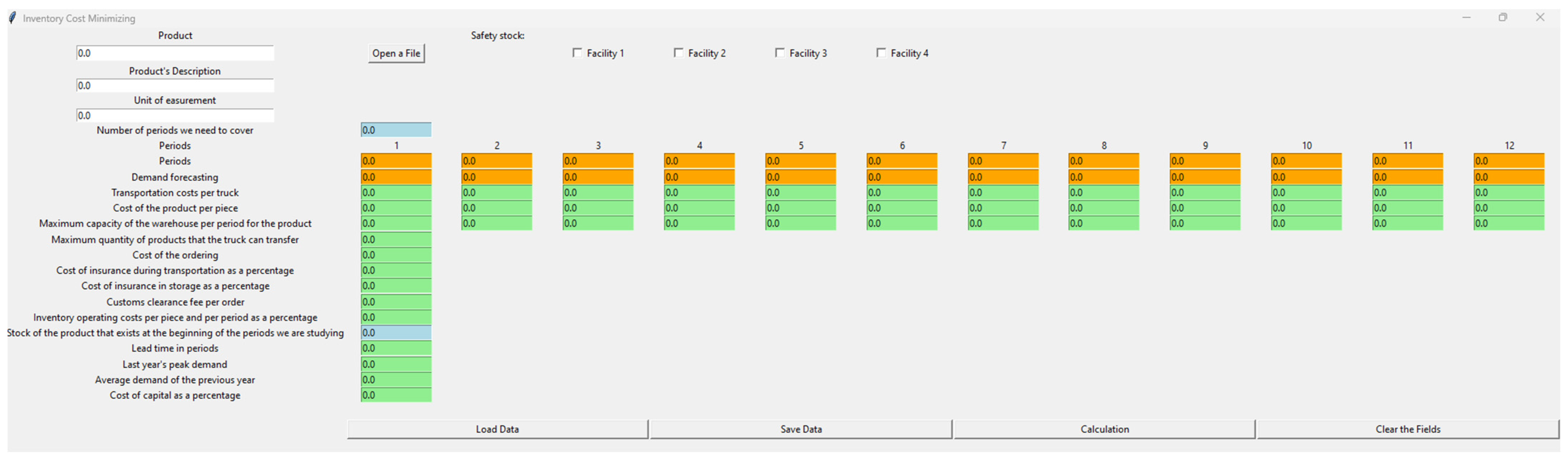
The proposed “ICM” tool appears in Figure 1. To illustrate the functionality and capabilities of the implemented tool, five different scenarios are presented below. Their description is shown in

Table 2. Description of the scenarios.

No.	Scenarios
1	A 6-period time horizon with no constraint on the maximum capacity of the warehouse.
2	Similar to Scenario 1 + constraint on the maximum capacity of the warehouse.
3	Similar to Scenario 1 + no holding costs.
4	Similar to Scenario 1 + 12-period time horizon and no holding costs.
5	Similar to Scenario 1 + 12-period time horizon.

.

• Scenario 1

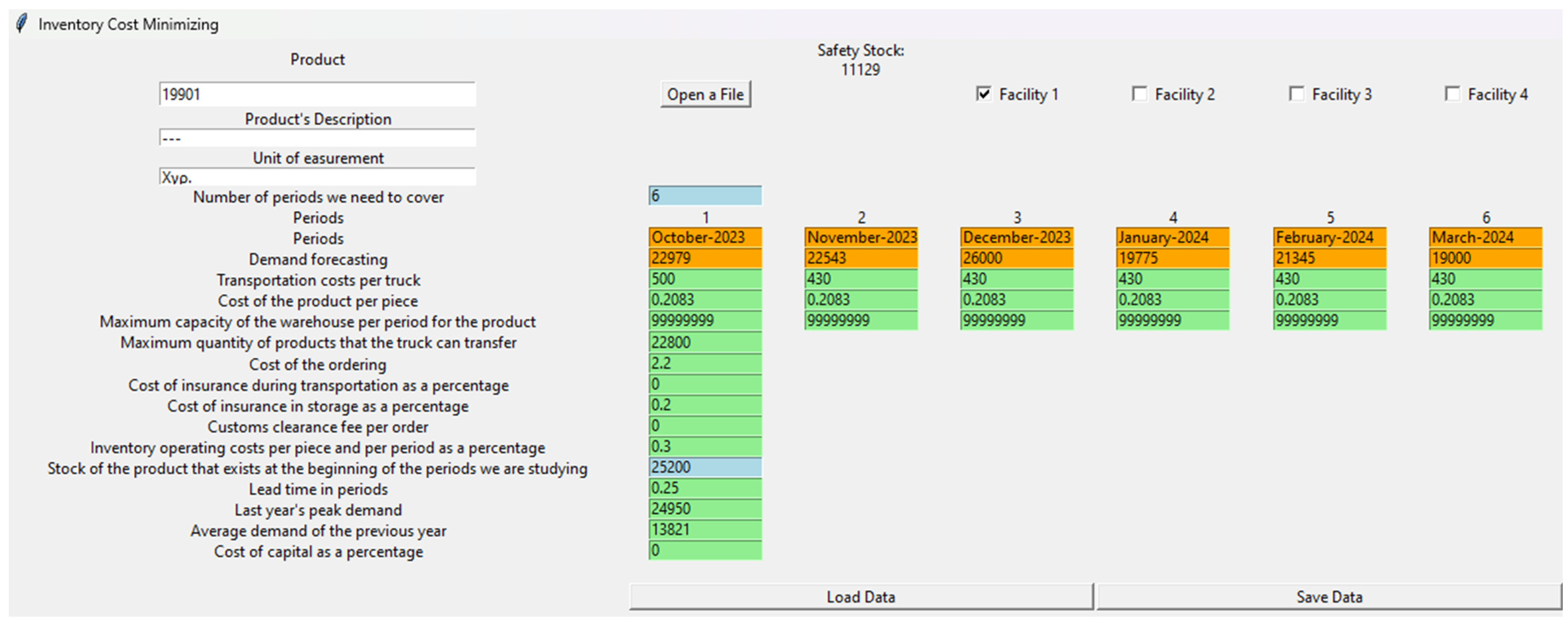
In Scenario 1 (Figure 2), the tool calculates the optimized order quantity and order time for a product and an order planning time horizon of six periods. According to the scenario, the forecasted demand for these six periods is 22,979 pcs, 22,534 pcs, 26,000 pcs, 19,775 pcs, 21,345 pcs, and 19,000 pcs, respectively. The capacity of the warehouse has no constraint, and the transportation cost is equal to 500 per truck for the first period and 430 per truck for the next five periods. The values of all variables for Scenario 1 are presented in Appendix A. The values of the decision variables regard a real-world case as they were collected (a) from an expert in inventory management working in the building and insulation materials industry; or (b) regarding the predicted demands from the demand forecasting system developed for the same building and insulation materials industry, as presented in the paper by Theodoridis and Tsadiras (2024) [27].

For Scenario 1, the proposed orders from the tool are exhibited in

Table 3. Results of Scenario 1.

Partially Loaded Truck Orders
Order ID	Order Time Period	Demand covering period(s)	Quantity (truck max capacity: 22,800 pcs)	Cost
1	0	1	1 truck with 8908 pcs	2355.54
2	1	1	1 truck with 22,543 pcs	5125.71
3	2	3	2 full trucks and 1 truck with 21,520 pcs	15,271.10
4	5	1	1 truck with 19,000 pcs	4387.70
Full-Truck Orders
Order ID	Order Time Period	Demand covering period(s)	Quantity in Trucks (truck capacity: 22,800 pcs)	Cost
1	0	1	1 full truck	5249.24
2	1	1	1 full truck	5179.24
3	2	1	1 full truck	5179.24
4	3	1	1 full truck	5179.24
5	4	1	1 full truck	5179.24
6	5	1	1 full truck	5179.24

. According to these, the following is observed:

(a)

For the case of partially loaded trucks, four orders are proposed at periods 0 (today), 1, 2, and 5. Each of these orders covers the demand of 1, 1, 3, and 1 period(s), respectively, with order quantity and costs shown in Table 2.

(b)

For the full-truck case, the tool advises the user to make one order each period. Each order covers the demand for 1 period, the order quantity is one full truck, and the cost is 5179.24 for each order, except for the first order, which costs 5249.24 due to the higher transportation cost of the first period that exists according to the scenario.

• Sensitivity Analysis of Scenario 1

The tool can serve as a sensitivity analysis tool through “what-if” scenarios, enabling users to examine the policy they could adopt as well as the cost implications associated with changing certain variables.

In this part of our study, we apply sensitivity analysis to the parameters of Scenario 1. Specifically, we vary one decision variable at a time, such that the number of orders proposed by the tool for the case of partially loaded trucks is altered. The altered parameters and the resulting outcomes are presented in the following

Table 4. Results of sensitivity analysis of Scenario 1.

Decision Variable	Range → No. of Orders
Maximum capacity of the warehouse per period for the product	[37,129, 68,580) → 6 [68,580, +∞) → 4
Customs clearance fee per order	[0, 145) → 4 [145, 667) → 3 [667, +∞) → 2
Inventory operating costs per piece and per period as a percentage	[0, 0.66) → 4 [0.66, +∞) → 6
Cost of capital as a percentage	[0, 0.21) → 4 [0.21, +∞) → 6
Cost of insurance in storage as a percentage	[0, 1.9) → 4 [1.9, +∞) → 6

.

As shown above, regarding the warehouse, the capacity of 68,580 serves as the threshold beyond which orders increase from 4 to 6 due to the lack of available space for product storage. In Table 4, it can be noticed that when “Maximum capacity of the warehouse per period for the product” or “Customs clearance fee per order” increases, the number of orders decreases to avoid additional costs. Conversely, for the remaining decision variables, as they increase, the number of orders also increases to prevent the business from inventorying, which entails additional holding costs. Such “what-if” scenarios can be very useful to users of the ICM tool since they can examine scenarios that they have in mind and apply only those that have positive consequences according to the ICM tool.

• Scenario 2

Scenario 2 is similar to Scenario 1, with the only difference being that the maximum capacity of the warehouse is now constrained to 45,600 pcs. The tool applies the proposed algorithms and, as shown in

Table 5. Results of Scenario 2.

Partially Loaded Truck Orders
Order ID	Order Time Period	Demand covering period(s)	Quantity (truck max capacity: 22,800 pcs)	Cost
1	0	1	1 truck with 8908 pcs	2355.54
2	1	1	1 truck with 22,543 pcs	5125.71
3	2	1	1 full truck and 1 truck with 3200 pcs	6275.80
4	3	1	1 truck with 19,775 pcs	4579.13
5	4	1	1 truck with 21,345 pcs	4876.16
6	5	1	1 truck with 19,000 pcs	4387.70
Full-Truck Orders
Order ID	Order Time Period	Demand covering period(s)	Quantity in Trucks (truck capacity: 22,800 pcs)	Cost
1	0	1	1 full truck	5249.24
2	1	1	1 full truck	5179.24
3	2	1	1 full truck	5179.24
4	3	1	1 full truck	5179.24
5	4	1	1 full truck	5179.24
6	5	1	1 full truck	5179.24

, advises the user, every different time period, to make one order with a specific quantity of the product, either for the case of partially loaded trucks or for the full-truck case. Comparing these orders to those of Scenario 1, it can be noticed that for the case of partially loaded truck orders, order no. 3 is not as high in quantity as that of Scenario 1 (two full trucks and one truck with 21,520 pcs in Scenario 1 vs. one full truck and one truck with 3200 pcs in Scenario 2) due to the warehouse maximum capacity constraint.

• Scenario 3

Scenario 3 is similar to Scenario 1, with the only difference being that there are no holding costs now (“Cost of insurance in storage as a percentage” and “Inventory operating costs per piece and per period as a percentage” are equal to 0). In this scenario, the tool proposes (see

Table 6. Results of Scenario 3.

Partially Loaded Truck Orders
Order ID	Order Time Period	Demand covering period(s)	Quantity (truck max capacity: 22,800 pcs)	Cost
1	0	1	1 truck with 8908 pcs	2355.54
2	1	5	4 full trucks and 1 truck with 17,463 pcs	24,787.50
Full-Truck Orders
Order ID	Order Time Period	Demand covering period(s)	Quantity in Trucks (truck capacity: 22,800 pcs)	Cost
1	0	1	1 full truck	5249.24
2	1	5	5 full trucks	25,896.20

) one order regarding the demand of the first period and a second order that regards the demands of all other periods. This can be justified by the fact that the transportation cost for the first period (EUR 500) is higher than that of the other periods (EUR 430). So, the first order covers the necessary quantity to cover the demand of the first order with a relatively expensive transportation cost, while the second order covers the remaining demand of the five periods with less expensive transportation (there are no holding costs or constraints on the maximum capacity of the warehouse).

• Scenario 4

Scenario 4 is similar to Scenario 1, having the following two differences: (a) it regards a planning time horizon of 12 periods, having the same levels of demands for the first six periods, zero demand for periods 7–9 and 11–12, and a demand of 100,000 pcs for period 10; and (b) there are no holding costs (“Cost of insurance in storage as a percentage” and “Inventory operating costs per piece and per period as a percentage” are equal to 0). Having no constraint in warehouse capacity and no holding costs, the tool proposes (see

Table 7. Results of Scenario 4.

Partially Loaded Truck Orders
Order ID	Order Time Period	Demand covering period(s)	Quantity (truck max capacity: 22,800 pcs)	Cost
1	0	1	1 truck with 8908 pcs	2355.54
2	1	11	9 full trucks and 1 truck with 3463 pcs	47,764.50
Full-Truck Orders
Order ID	Order Time Period	Demand covering period(s)	Quantity in Trucks (truck capacity: 22,800 pcs)	Cost
1	0	1	1 full truck	5249.24
2	1	11	9 full trucks	46,613.16

), similarly to Scenario 3, for both cases of partially loaded trucks and full trucks, one order at the beginning of the planning time horizon to cover the demand of the 1st period and one more order for the demand of the remaining 11 periods.

• Scenario 5

Scenario 5 is similar to Scenario 4, with the only difference being that there are holding costs now. As exhibited in Table 6, for the partially loaded truck case, the tool proposes five orders (at periods 0, 1, 2, 5, and 9), each covering the demand of 1 up to 4 periods (demands for 1, 1, 3, 4, and 3 periods, respectively). For the full-truck case, the tool proposes seven orders, also shown in

Table 8. Results of Scenario 5.

Partially Loaded Truck Orders
Order ID	Order Time Period	Demand covering period(s)	Quantity (truck max capacity: 22,800 pcs)	Cost
1	0	1	1 truck with 8908 pcs	2355.54
2	1	1	1 truck with 22,543 pcs	5125.71
3	2	3	2 full trucks and 1 truck with 21,520 pcs	15,271.10
4	5	4	1 truck with 19,000 pcs	4387.70
5	9	3	4 full trucks and 1 truck with 8800 pcs	22,980
Full-Truck Orders
Order ID	Order Time Period	Demand covering period(s)	Quantity in Trucks (truck capacity: 22,800 pcs)	Cost
1	0	1	1 full truck	5249.24
2	1	1	1 full truck	5179.24
3	2	1	1 full truck	5179.24
4	3	1	1 full truck	5179.24
5	4	1	1 full truck	5179.24
6	5	4	1 full truck	5179.24
7	9	3	4 full trucks	20,716.96

, each corresponding to a period with a non-zero forecasted demand.

6. Summary, Conclusions, and Future work

In this paper, after a literature review on Economic Order Quantity (EOQ) models and the Wagner–Whitin algorithm and all its variants, we present an extended real-world lot-sizing problem and an algorithmic solution. This algorithm extends the Wagner–Whitin method and takes into consideration all the relevant necessary data, i.e., costs, capacity of the warehouse, safety stock, and price of the ordering product per period.

The output of the algorithm is the ordering time and ordering quantity for orders covering up to 12 periods of time (e.g., months). We also present a variation of the algorithm to cover the case of full-truck orders only. These algorithms are implemented using the Python programming language and the Tkinter library. The tool that is created provides a user-friendly graphical environment where the user can experiment with different scenarios. Several such scenarios are exhibited in Section 5, where the functionality of the tool, the different parameters, and the results are presented, as well as the sensitivity analysis of Scenario 1.

Our plan is to extend the algorithms presented in this study to cover the case of multiple suppliers per ordering product. Another plan is to extend the proposed algorithms in such a way that they will offer optimal orders for cases in which each truck can carry not one but various different products from the same supplier.

References

- Lolli, F.; Balugani, E.; Ishizaka, A.; Gamberini, R.; Rimini, B.; Regattieri, A. Machine learning for multi-criteria inventory classification applied to intermittent demand. Prod. Plan. Control 2019, 30, 76–89. [Google Scholar] [CrossRef]
- Karimi, B.; Ghomi, S.F.; Wilson, J.M. The capacitated lot sizing problem: A review of models and algorithms. Omega 2003, 31, 365–378. [Google Scholar] [CrossRef]
- Wagner, H.M.; Whitin, T.M. Dynamic version of the economic lot size model. Manag. Sci. 1958, 5, 89–96. [Google Scholar] [CrossRef]
- Nahmias, S.; Olsen, T.L. Production and Operations Analysis; Waveland Press: Long Grove, IL, USA, 2015. [Google Scholar]
- Bushuev, M.A.; Guiffrida, A.; Jaber, M.Y.; Khan, M. A review of inventory lot sizing review papers. Manag. Res. Rev. 2015, 38, 283–298. [Google Scholar] [CrossRef]
- Muckstadt, J.A.; Sapra, A. Principles of Inventory Management: When You Are Down to Four, Order More; Springer Science & Business Media: Berlin/Heidelberg, Germany, 2010. [Google Scholar]
- Saydam, C.; Evans, J.R. A comparative performance analysis of the Wagner-Whitin algorithm and lot-sizing heuristics. Comput. Ind. Eng. 1990, 18, 91–93. [Google Scholar] [CrossRef]
- Drexl, A.; Kimms, A. Lot sizing and scheduling—Survey and extensions. Eur. J. Oper. Res. 1997, 99, 221–235. [Google Scholar] [CrossRef]
- Evans, J.R. An efficient implementation of the Wagner-Whitin algorithm for dynamic lot-sizing. J. Oper. Manag. 1985, 5, 229–235. [Google Scholar] [CrossRef]
- Wagelmans, A.; Van Hoesel, S.; Kolen, A. Economic lot sizing: An O (n log n) algorithm that runs in linear time in the Wagner-Whitin case. Oper. Res. 1992, 40 (Suppl. 1), S145–S156. [Google Scholar] [CrossRef]
- Heady, R.B.; Zhu, Z. An improved implementation of the Wagner-Whitin Algorithm. Prod. Oper. Manag. 1994, 3, 55–63. [Google Scholar] [CrossRef]
- Sajadi, S.; Arianezhad, M.G.; Sadeghi, H.A. An Improved WAGNER-WHITIN Algorithm. Int. J. Ind. Eng. Prod. Res. 2009, 20, 117–123. [Google Scholar]
- Chowdhury, N.T.; Baki, M.F.; Azab, A. Dynamic economic lot-sizing problem: A new O (T) algorithm for the Wagner-Whitin model. Comput. Ind. Eng. 2018, 117, 6–18. [Google Scholar] [CrossRef]
- Vargas, V. An optimal solution for the stochastic version of the Wagner–Whitin dynamic lot-size model. Eur. J. Oper. Res. 2009, 198, 447–451. [Google Scholar] [CrossRef]
- Richter, K. Remanufacturing Planning by Reverse Wagner; Whitin Models, Discussion Paper 104; Department of Economics, European University Viadrina: Frankfurt, Germany, 1997. [Google Scholar]
- Richter, K.; Weber, J. The reverse Wagner/Whitin model with variable manufacturing and remanufacturing cost. Int. J. Prod. Econ. 2001, 71, 447–456. [Google Scholar] [CrossRef]
- Gulecyuz, S.; O’Sullivan, B.; Tarim, S.A. A Heuristic Method for Perishable Inventory Management under Non-Stationary Demand. In Proceedings of the International Workshop on Lot-Sizing-IWLS’2023, Cork, Ireland, 23–25 August 2023; p. 49. [Google Scholar]
- Gharaei, A.; Hoseini Shekarabi, S.A.; Karimi, M. Optimal lot-sizing of an integrated EPQ model with partial backorders and re-workable products: An outer approximation. Int. J. Syst. Sci. Oper. Logist. 2023, 10, 2015007. [Google Scholar] [CrossRef]
- Metzker, P.; Thevenin, S.; Adulyasak, Y.; Dolgui, A. Robust optimization for lot-sizing problems under yield uncertainty. Comput. Oper. Res. 2023, 149, 106025. [Google Scholar] [CrossRef]
- Forel, A.; Grunow, M. Dynamic stochastic lot sizing with forecast evolution in rolling-horizon planning. Prod. Oper. Manag. 2023, 32, 449–468. [Google Scholar] [CrossRef]
- Benmamoun, Z.; Fethallah, W.; Ahlaqqach, M.; Jebbor, I.; Benmamoun, M.; Elkhechafi, M. Butterfly Algorithm for Sustainable Lot Size Optimization. Sustainability 2023, 15, 11761. [Google Scholar] [CrossRef]
- Rojas, F.; Leiva, V.; Huerta, M.; Martin-Barreiro, C. Lot-size models with uncertain demand considering its skewness/kurtosis and stochastic programming applied to hospital pharmacy with sensor-related COVID-19 data. Sensors 2021, 21, 5198. [Google Scholar] [CrossRef] [PubMed]
- Popović, D.; Bjelić, N.; Vidović, M.; Ratković, B. Solving a Production Lot-Sizing and Scheduling Problem from an Enhanced Inventory Management Perspective. Mathematics 2023, 11, 2099. [Google Scholar] [CrossRef]
- Dimoudis, D.; Vafeiadis, T.; Nizamis, A.; Musiari, E.; Ziliotti, L.; Ioannidis, D.; Tzovaras, D. A holistic framework for production scheduling in Industry 4.0. In Proceedings of the 2023 19th International Conference on Distributed Computing in Smart Systems and the Internet of Things (DCOSS-IoT), Pafos, Cyprus, 19–21 June 2023; pp. 269–276. [Google Scholar]
- Zhang, Z.; Gao, C.; Luedtke, J. New valid inequalities and formulations for the static joint Chance-constrained Lot-sizing problem. Math. Program. 2023, 199, 639–669. [Google Scholar] [CrossRef]
- Dey, B.K.; Seok, H. Intelligent inventory management with autonomation and service strategy. J. Intell. Manuf. 2024, 35, 307–330. [Google Scholar] [CrossRef] [PubMed]
- Theodoridis, G.; Tsadiras, A. Retail Demand Forecasting: A Multivariate Approach and Comparison of Boosting and Deep Learning Methods. Int. J. Artif. Intell. Tools 2024. [Google Scholar] [CrossRef]
Disclaimer/Publisher’s Note: The statements, opinions and data contained in all publications are solely those of the individual author(s) and contributor(s) and not of MDPI and/or the editor(s). MDPI and/or the editor(s) disclaim responsibility for any injury to people or property resulting from any ideas, methods, instructions or products referred to in the content. |
© 2024 by the authors. Licensee MDPI, Basel, Switzerland. This article is an open access article distributed under the terms and conditions of the Creative Commons Attribution (CC BY) license (https://creativecommons.org/licenses/by/4.0/).