Article

A Data-Driven Approach to Set-Theoretic Model Predictive Control for Nonlinear Systems †

by
Francesco Giannini
and
Domenico Famularo
*,‡
Department of Computer Engineering, Modeling, Electronics and Systems (DIMES), Università della Calabria, Via P. Bucci, 42-C, 87036 Rende, Italy
*
Author to whom correspondence should be addressed.
This article is a revised and expanded version of a paper entitled: Francesco Giannini, et al. Set-theoretic receding horizon control for nonlinear systems: a data-driven approach, which was presented In Proceedings of the IEEE EUROCON 2023—20th International Conference on Smart Technologies, Torino, Italy, 6–8 July 2023.
These authors contributed equally to this work.
Information 2024, 15(7), 369; https://doi.org/10.3390/info15070369
Submission received: 21 May 2024 / Revised: 18 June 2024 / Accepted: 21 June 2024 / Published: 23 June 2024
(This article belongs to the Special Issue Second Edition of Predictive Analytics and Data Science)

Abstract

:
In this paper, we present a data-driven model predictive control (DDMPC) framework specifically designed for constrained single-input single-output (SISO) nonlinear systems. Our approach involves customizing a set-theoretic receding horizon controller within a data-driven context. To achieve this, we translate model-based conditions into data series of available input and output signals. This translation process leverages recent advances in data-driven control theory, enabling the controller to operate effectively without relying on explicit system models. The proposed framework incorporates a robust methodology for managing system constraints, ensuring that the control actions remain within predefined bounds. By means of time sequences, the controller learns the underlying system dynamics and adapts to changes in real time, providing enhanced performance and reliability. The integration of set-theoretic methods allows for the systematic handling of uncertainties and disturbances, which are common when the trajectory of a nonlinear system is embedded inside a linear trajectory state tube. To validate the effectiveness of our DDMPC framework, we conduct extensive simulations on a nonlinear DC motor system. The results demonstrate significant improvements in control performance, highlighting the robustness and adaptability of our approach compared to traditional model-based MPC techniques.

1. Introduction

Model predictive control (MPC) is a powerful control technique which relies on repeatedly solving an open-loop optimal control problem [1]. The key advantages of MPC compared to other control methods are its applicability to nonlinear systems, the possibility to include constraints on system variables, and desirable closed-loop guarantees on stability and performance. MPC is essentially a model-based control strategy, but the model derivation is typically a laborious process, demanding expert knowledge. This challenge has spurred growing interest in developing controllers directly from data, bypassing the need for explicit model knowledge. Model predictive control strategies based on a data-driven approach (DDMPC) represent, in fact, an emerging paradigm that harnesses the vast amounts of data generated by modern systems to enhance control strategies without necessitating explicit mathematical models of a plant [2,3,4,5,6]. This paradigm shift allows for the development of robust control methods even in scenarios where obtaining an accurate mathematical model is challenging or impractical and has garnered significant interest due to several motivations stemming from its advantages over traditional model-based control methods (see [7] for a general discussion on the matter). One of the most relevant aspects is the reduced modeling effort since a data-driven approach circumvents the need for complex mathematical modeling, thus diminishing the effort required for controller design [8]. Connected to this is the adaptability of a data-driven MPC scheme to complex and nonlinear systems where traditional models may be inaccurate or impractical [9]. Model uncertainties and disturbances can also be efficiently managed, making a DDMPC scheme robust to modeling errors and external disturbances; in addition, DDMPC allows for real-time adaptation and learning from dynamic environments, thereby enhancing controller performance over time [10]. Like other non-model-based methods, DDMPC offers scalability and generalization capabilities, enabling controllers to be applied across different systems and scenarios. This facilitates the integration of domain knowledge with data-driven insights, leading to more effective control strategies [11]. DDMPC presents, then, a promising scenario for advancing control theory and practice across various domains such as robotics [12], manufacturing [13], energy systems [10], and transportation [14]. The common denominator is the practical relevance and impact of DDMPC in addressing real-world control problems and improving system performance, eliminating the need for explicit mathematical models [15,16].
Of interest for us are algorithmic schemes tailored specifically for DDMPC based on data-driven optimization algorithms, reinforcement learning-based control strategies, and adaptive learning algorithms: these computational schemes are designed to tackle the challenges posed by real-world data, ensuring robust and efficient control performance [17,18]. Performance evaluations and comparisons between DDMPC and traditional model-based control methods have been conducted: the idea is assess the advantages and limitations of DDMPC in terms of control quality, robustness, computational efficiency, and adaptability to changing environments (see [19]). DDMPC relies on the basis that learning from data approaches is of paramount interest mainly due to the strict link with artificial intelligence [20,21] and that this relation can be exploited for control design purposes; see [22,23] and references therein. Accordingly, it is of paramount relevance to comprehend how data-driven schemes can substitute model-based approaches while preserving structural system properties such as controllability and observability, alongside algorithmic properties like feasibility and closed-loop stability. The contribution in [24] provides a crucial result for linear systems: all the trajectories of a linear system can be represented by a finite set of adequately excited system trajectories. Starting from this statement, in [25], the existence of a parametrization of feedback control systems that allows one to reduce the stabilization problem to an equivalent data-dependent linear matrix inequality (LMI) is proven. A more recent contribution [26], even if not directly classifiable within a DDMPC context, is of interest since it analyzes a data-driven simulation method applied to SISO bilinear systems whose trajectory is embedded in the behavior of an LTI system. In the author’s words, the key issue is an embedding result that is of independent interest: the behavior of a nonlinear system (in this case bilinear) is included in the behavior of a linear time-invariant system. Notably, these findings establish the existence of a linear time-invariant (LTI) embedding for a SISO nonlinear system.

Manuscript Contribution

Based on these premises, in this paper, which is an extension of [27] in terms of complete introduction rewriting, linear embedding technicality clarification, and the deepest analysis of the more recent literature by adding two new numerical examples with comparisons with a model-based competitor nonlinear MPC scheme (absent in [27]), set-theoretic and deep learning arguments are merged within a data-driven receding horizon control (RHC) framework tailored for nonlinear single-input single-output (SISO) systems. Specifically, we adapt the low-demanding algorithm outlined in [28], which is the MPC core of our approach, to suit within a data-driven context by extending the results from [25,26] by proving the existence of a data-driven multi-model polytopic state-tube which entraps the trajectories of the nonlinear SISO model describing the plant (polytopic embedding) [29]. Then, the so-called terminal pair complying with the available equilibrium is designed by exploiting feedback linearization arguments and a proper customization of the regulation linear controller of [25] by also adding data-driven formulas for input and output constraints. We resort to a deep learning data-driven modeling technique where a nonlinear or uncertain system is represented as a convex combination of linear models. Essentially, the system behavior is described by a convex set of polytopes, with each polytope representing a possible linear dynamic of the system. This technique has proven extremely useful for analysis and controller design problems for nonlinear systems and/or linear systems with uncertainties or parameter variations [30]. Through the authors’ best intention and acknowledgment, the contribution represents, in contrast to the cited literature, a first step towards mixing an efficient and computationally low-demand scheme with the possible potentiality of data-driven control. To prove the benefits of the proposed scheme, two numerical experiments have been proposed: the first one is the angular velocity regulation problem of a nonlinear DC motor model, and the second one is the Reactant concentration regulation problem for a Continuous Stirred Tank Reactor (CSTR) nonlinear model. As previously stated, for both examples, comparisons in terms of regulation performance (controlled variable time trend) with a model-based ad hoc nonlinear MPC scheme [31] have been shown and discussed in detail.

2. Notations, Definitions, and Problem Formulation

0 d and I r denote the vector of d zero entries and the identity matrix of order r , respectively.
The convex hull [30] of a finite set of real matrices A = A i R ν × μ i = 1 L is the set of all convex combinations of the elements of A
C o A i i = 1 L = λ 1 A 1 + + λ 1 A L , λ i 0 , λ 1 + + λ L = 1
C o A i i = 1 L is defined as a polytope of A , and A i , i = 1 , , L denote the related vertices.
Consider the following discrete time-linear, time-varying system:
x ( t + 1 ) = Φ ( λ ( t ) ) x ( t ) + G ( λ ( t ) ) u ( t )
where t Z Z + : = { 0 , 1 , . . . } , x ( t ) I R n is the state, u ( t ) I R m the control input, and λ ( t ) is a time-varying parameter, in general not known in advance, belonging to the following set t Z Z + :
Λ : = λ I R L : j = 1 L λ j = 1 , λ j 0
( Φ j , G j ) denotes the polytope vertex, viz. ( Φ , G ) C o Φ j , G j j = 1 L .
Definition 1 
([32]). A set Ξ X is said to be robust positively invariant (RPI) for (2) and (3) under (5) if there exists a control law u ( t ) : = h ( x ( t ) ) U such that x ( 0 ) Ξ one has
Φ ( λ ( t ) ) x ( t ) + G ( λ ( t ) ) h ( x ( t ) ) Ξ , λ ( t ) Λ , t Z +
Given a set S X × Y I R n × I R m , the projection of the set S onto X is defined as Proj X ( S ) : = x X | y Y s . t . ( x , y ) S .

Problem Formulation

In the sequel, we consider a plant described by a discrete time-invariant nonlinear system model state space representation:
x ( t + 1 ) = f ( x ( t ) , u ( t ) ) y ( t ) = C x ( t )
where x ( t ) I R n is the state of the system, u ( t ) I R m is the command input, and y ( t ) I R p is the measurement vector with C I R p × n in the output matrix (linear map). Moreover, it is assumed that the plant actuator input and states are prescribed to satisfy the following constraints:
u ( t ) U : = { u I R m | u T u u ¯ 2 } , t 0 x ( t ) X : = { x I R n | x T x x ¯ 2 } , t 0 ,
with U , X convex and compact subsets of I R m and I R n , respectively. The following assumption on the nonlinear map f ( · , · ) is given:
Assumption 1. 
The one-step-ahead transition-state map f : I R n × I R m I R n is uniformly Lipschitz in ( x , u ) X × U , i.e.,
f ( x , u ) f ( x ^ , u )   γ x x x ^ , ( x , x ^ ) X × X ,
f ( x , u ) f ( x , u ^ )   γ u u u ^ , ( u , u ^ ) U × U ,
with γ u , γ x I R , γ u 0 , γ x 0 as known Lipschitz constants.
Moreover, it is assumed that 0 n I R n is an equilibrium point for (4) with u = 0 m , i.e., f ( 0 n , 0 m ) = 0 n .
The goal is to find a state feedback regulation strategy u ( t ) = g ( x ( t ) ) that asymptotically stabilizes the system described by (4) to the origin while satisfying the constraints given in (5). The proposed approach can be outlined as follows: assume there exists a sequence of N + 1 ( N > 0 ) regions T i i = 0 N , where T 0 is an arbitrary target set with an associated stabilizing state feedback law u 0 ( x ) U (refer to [28] for details on this strategy). The objective is to compute an admissible control strategy that can drive any initial state x ( 0 ) i = 0 N T i to the terminal (target) robust positively invariant (RPI) set T 0 in finite time. Thus, the problem statement is as follows:
  • MPC Problem—Given the nonlinear system (4), a sequence of regions { T i } i = 0 N and an initial state x ( 0 ) i = 0 N T i , compute at each time instant t and on the basis of the current state x ( t ) a control strategy, compatible with (5), such that there exists a finite time instant t ¯ 0 so that x ( t ¯ ) T 0 is achieved while a performance index is minimized.

3. Background

In this section, we summarize the set-theoretic receding horizon control (RHC) scheme for addressing the MPC Problem for linear system models (2). Using the ellipsoidal calculus methods [33], the target set T 0 , which satisfies RPI Definition 1, is initially computed. Subsequently, the algorithm’s working-state region is extended by deriving sets of states that can be steered into T 0 within a finite number of steps. Specifically, the pair ( K , E ) , with E R n being an ellipsoidal set and K R m × n the gain matrix of the stabilizing control law u ( t ) = K x ( t ) , satisfies
( Φ j + G j K ) E E X , j = 1 , , L ,
and can be computed by solving the following linear matrix inequality (LMI) optimization:
min Q , Y , ρ , ρ
subject to
1 x ( t ) T x ( t ) Q 0 ,
Q * * * Φ j Q + G j Y Q * * R x 1 / 2 Q 0 ρ I n * R u 1 / 2 Y 0 0 ρ I m 0 j = 1 , , L ,
Q * Φ j Q + G j Y x ¯ 2 I n 0 , j = 1 , , L ,
u ¯ 2 I n * Y T Q 0 , P = ρ Q 1 , K = Y Q 1
As a consequence,
E : = { x I R n | x T P x 1 } , Q = Q T 0 ,
is a RPI region for the closed-loop collection of states
x ( t + 1 ) = ( Φ ( λ ( t ) ) + G ( λ ( t ) ) K ) x ( t ) , λ ( t ) Λ ,
complying with the prescribed constraints, viz. E X and K E U .
Regarding the set sequence { T i } , it is computed using the concept of the one-step state-ahead controllable set:
Definition 2. 
Given the set T X , the predecessor set P r e ( T ) is the set of states for which there exists a causal control u ( t ) U such that the resulting one-step state transition lies within T . Specifically,
P r e T : = { x X : u U : Φ j x + G j u T , j = 1 , , L }
Let E be the target set; it is possible to determine the sets of states that are i-step controllable to E using the following recursion (see [32]):
T 0 : = E , T i : = P r e ( T i 1 ) i > 0
The recursion (13) can be implemented via LMIs leading to inner ellipsoidal approximations of { T i } . Notice that
{ x X | u U : λ Λ , Φ ( λ ) x + G ( λ ) u T i } = { x X | u U : j = 1 , , L , Φ j x + G j u T i } { x X | u U : j = 1 , , L , Φ j x + G j u I n [ T i ] } = Proj x [ x u ] | u U and j = 1 , , L , [ x u ] E ˜ i 1 j
where I n [ · ] is the inner ellipsoidal approximation operator and E ˜ i 1 the ellipsoidal set defined in the extended space ( x , u ) . Then, by expressing without loss of generality the constraint set U as the intersection of ellipsoidal sets (see [28,33] for details)
U = i E i U
one obtains
{ x X | u U : λ Λ , Φ ( λ ) x + G ( λ ) u T i } Proj x I n j = 1 L E ˜ i 1 i ( I R n × E i U ) = : E i
Hence, an MPC Algorithm 1 can be straightforwardly outlined:
Algorithm 1 Set-theoretic Model Predictive Control (ST-MPC) Algorithm
Input:  { E i } i = 0 N ;
Output:  u ( t )
  1: Compute  i ( t ) = min { i : x ( t ) E i } ;
  2: if  i ( t ) = 0  then  u ( t ) = K x ( t ) ;
  3: else
                                                                                  u ( t ) = arg min J i ( t ) ( x ( t ) , u )                                                                                   such that                                                                                   Φ j x + G j u E i 1 , j = 1 , , L ; u U
  4: end if
  5: Apply u ( t ) ;
  6: t t + 1 ; Goto Step 1;
Notice that the cost J i ( t ) ( x ( t ) , u ) can be arbitrarily chosen without affecting the feasibility and closed-loop stability of the Algorithm 1; see [28] for technical details.

4. A Data-Driven Low-Demand Algorithm

In the following, attention will be restricted to single-input single-output (SISO) systems, i.e., m = p = 1 in (4). Furthermore, following the reasoning outlined in [25], it is assumed that the system state is fully accessible. The novel approach here consists in tailoring the Algorithm 1 within a data-driven scenario, which involves characterizing the terminal pair ( K , E ) and the family { T i } for the nonlinear context by deriving the polytopic model, instrumental for Algorithm 1 by means of a machine learning-based algorithm.
To this end, the following ingredients will be exploited:
  • Data-based state-feedback control [25];
  • Linear time-invariant embedding for SISO nonlinear models [26].

4.1. Stabilizing Control and Positively Invariant Set

Under the hypothesis that the equilibrium ( x ¯ , u ¯ ) is known a priori, feedback linearization arguments can be used together with the [25] derivations adapted to comply with the prescribed state and input constraints (5).
Let
U 0 , 1 , T : = [ u d ( 0 ) u d ( 1 ) u d ( T ) ] X 0 , T : = [ x d ( 0 ) x d ( 1 ) x d ( T ) ] X 1 , T : = [ x d ( 1 ) x d ( 2 ) x d ( T ) ]
where the subscript d accounts for sample data. Under the hypothesis that the system has linear time-invariant representation, in [25], it has been proved that
x ( t + 1 ) = X 1 , T U 0 , 1 , T ¯ X 0 , T u ( t ) x ( t )
with † being the Penrose pseudo inverse operator. Then, the following linear system description comes out:
[ Φ G ] = X 1 , T U 0 , 1 , T ¯ X 0 , T
In what follows, the concept of a persistently exciting input sequence is exploited.
Definition 3. 
A persistently exciting input sequence u d , [ 0 , T 1 ] of order n + 1 satisfies the following condition:
R a n k U 0 , 1 , T ¯ X 0 , T = n + 1
Therefore, for the linear system description (17) subject to (5), a stabilizing state feedback controller and the associated positively invariant region can be achieved under the following result.
Theorem 1. 
Assume that (18) holds true. Then, the constrained linear system (17), (5) is asymptotically stabilizable by
K = U 0 , 1 , T Y ( X 0 , T Y ) 1
with
E = { x I R n | x T ( X 0 , T Y ) 1 x 1 } X
a positively invariant region for the closed-loop trajectories such that K E U , if the following matrix inequalities conditions are satisfied:
X 1 , T Y ( X 0 , T Y ) 1 Y T X 1 , T T X 0 , T Y < 0
X 0 , T Y > 0
U 0 , 1 , T Y = K X 0 , T Y
( X 0 , T Y ) 1 Y T U 0 , 1 , T T U 0 , 1 , T Y ( X 0 , T Y ) 1 u ¯ 2 I
( X 0 , T Y ) 1 Y T X 1 , T T X 1 , T Y ( X 0 , T Y ) 1 x ¯ 2 I
Proof. 
By exploiting the arguments developed in [25], the proof straightforwardly follows by introducing an auxiliary symmetric and positive defined matrix P such that
X 0 , T Y = P U 0 , 1 , T Y = K P
   □
Remark 1. 
Notice that (21)–(25) is a non-convex bilinear matrix inequality (BMI) feasibility problem in the matrix variable P . Although computationally complex, it can be addressed off-line via ad hoc BMI local solvers (see PENBMI [34] as an example).

4.2. Polytopic Embedding and Data-Set Machine Learning-Based Algorithm

A polytopic linear difference inclusion (PLDI) description of the nonlinear system (4) is first derived [30]. In the present context, this can be achieved thanks to a very recent result outlined in [26]. There, it is proved (Lemma 11, pg. 1104) that the state trajectories resulting from (4) can be embedded into an linear time-invariant (LTI) system in an extended state/input space. This argument makes it possible to consider a more complex PLDI instead of a single LTI system:
F = x + X | x + = Φ x + G u , [ Φ , G ] C o ( { [ Φ 1 G 1 ] , , [ Φ L G L ] } ) , ( x , u ) X × U
such that all ( x , u ) X × U
f ( x , u ) F
(all the state successors f ( x , u ) according to (4) are entrapped inside F e x t ). The matrix vertices [ Φ i G i ] , i = 1 , , L have been computed by a machine learning-based approach [35] which is proven to converge w.p.1 to the desired polytope C o ( { [ Φ 1 G 1 ] , , [ Φ L G L ] } ) as the number of episodes tends to be arbitrarily large. To this end, the following iterative machine learning-based scheme, whose flowchart is depicted in the following Figure 1, is introduced:
The following definition, instrumental for the scheme in Figure 1, states how the state/equilibrium pair is managed:
Definition 4. 
An input-state pair ( u s , x s ) I R m + n is an equilibrium pair of the nonlinear system (4) if the sequence { u ¯ ( t ) , x ¯ ( t ) } t 0 = ( u s , x s ) is a an admissible trajectory of (4).
Let S S ˜ be the set of matrix pairs [ Φ i , G i ] , i = 1 , , r , characterizing the linearized model of (4) around the equilibrium ( u e q i , x e q i ) . Then, the iterative machine learning-based algorithm sketched in Figure 1 is capable of deriving a PLDI (26) and is detailed here.
According to Definition 4, a set of equilibrium points { ( u e q i , x e q i ) } i = 1 r is determined by exhaustive research on the admissible system space U × X . Then, the data-based open-loop linearized couple [ Φ i G i ] is computed under the hypothesis that the equilibrium input u e q i is perturbed with zero mean white Gaussian noise so that the rank condition (18) holds. As a consequence, a persistently exciting input sequence ( u ˜ e q i ) [ 0 , T 1 ] is generated and the sequence of Equations (15)–(17) is then performed. Hence, a convex hull S S ˜ of the achieved dynamic/actuator matrix pairs is derived. Next, the well-posedness of S S ˜ must be checked: this is achieved by a Monte Carlo approach [36] by computing sequences of state trajectories { u s , x s i ( t ) } i = 1 N s and checking their membership to the state trajectory tube arising from the candidate embedding S S ˜ . If (26) holds true, then the procedure ends; otherwise, a new equilibrium is added for updating S S ˜ .
All the above developments allow us to write down the following computable Algorithm 2:
Algorithm 2 Iterative Machine Learning (IML) Algorithm
  1: Find { ( u e q i , x e q i ) } i = 1 r , via an exhaustive search on the space U × X ;
  2: Perturb the equilibrium inputs u e q i , i = 1 , , r , and generate the persistently exciting input sequence ( u ˜ e q i ) [ 0 , T 1 ] , i = 1 , , r , comply with (18);
  3: Apply Formulas (15)–(17) and obtain the data-based open-loop realization [ Φ i G i ] , i = 1 , , r ;
  4: Compute the convex hull
S S ˜ : = C o ( { [ Φ 1 G 1 ] , , [ Φ r G r ] } )
  5: Perform Monte carlo simulations: compute sequences of state trajectories { u s , x s i ( t ) } i = 1 N s and verify
x s i ( t ) S S ˜ , i ;
  6: if YES then Exit;
  7: else
  8:      Find a new equilibrium ( u e q r + 1 , x e q r + 1 ) ; r r + 1 ;
  9: end if
10: Goto Step 4 and update  S S ˜ ;

5. Illustrative Examples

In this section, we present two examples that illustrate the benefits of the proposed Algorithm 1 endowed with the machine learning Algorithm 2. The data-driven MPC algorithm will be contrasted in terms of regulation performance results with an ad hoc model based on the nonlinear MPC scheme, NMPC [31]. For both these examples, the following solvers have been used:
  • Algorithm 1
    Yalmip parser (available at the following: https://yalmip.github.io/download/ (accessed on 20 May 2024))/MOSEK © Optimization package (LMI procedures).
    MATLAB Reinforcement Learning toolbox © and the MATLAB Deep learning toolbox © (Algorithm 2).
  • fmincon MATLAB Optimization Toolbox © function used for the NMPC competitor.
A software repository related to Set Theoretic Data-Driven MPC can be found at the following https://github.com/PreCyseGroup/Data-Driven-ST-MPC (accessed on 20 May 2024).

5.1. DC Motor

In this example, we will consider the angular speed regulation of a separately excited DC motor nonlinear model [37]. Nonlinearities come from cross-product terms in the state space description, and the result is an inverse bond in the steady-state relationship between the control input and the regulated state variable. The model is as follows:
d I f d t = R f L f I f ( t ) + 1 L f V f ( t ) d I a d t = R a L a I a ( t ) K m L f L a ω ( t ) I a ( t ) + 1 L a V a ( t ) d ω d t = B m J m ω ( t ) + K m L a L f J m ω ( t ) I f ( t ) I a ( t ) 1 J m τ ( t )
where the following definitions apply:
  • I f and I a are the field and armature currents, and V f and V a are the related voltages;
  • ω is the shaft rotor angular speed;
  • τ L is the shaft rotor torque load;
and the systems parameters are
  • R f = 5 Ω , L f = 1 H , which are the field resistance/inductance, and R a = 10 Ω , L a = 1 H , which are the armature resistance/inductance;
  • J m = 0.2 Kg m 2 , B m = 0.011 Kg m 2 sec , which are the inertia and friction coefficient;
  • K m = 30 N m A 2 , which is the motor torque constant.
Note that the voltage and shaft rotor torque load inputs are linear terms inside the system flow, whereas the zero input is a nonlinear map in the system variables. This is not so uncommon when deriving a mathematical model from a phenomenon by resorting to basic physics laws, since the external sources (forces/torques, voltages, external flows, etc.) do enter in a linear fashion inside the system flow. Also, the presence of a linear input term is a good test to check if the input matrix of the obtained polytopic embedding is compliant with the physical nonlinear model at hand.
The proposed control strategy adheres to a standard two-loop approach, i.e., the motor is operated in the following way: the inner controller is in charge of imposing a prescribed constant field current I f , r e f = 4 A , and the external loop regulates the behavior of the angular speed by considering V a ( t ) as the control input and τ L ( t ) as a disturbance which for nominal operating conditions is kept constant to 18 N m . The inner loop is characterized by a simple, fast first-order controller:
d V f d t = 25 V f ( t ) + 1250 ( I f , r e f I f ( t ) )
and the resulting nonlinear model is then characterized by a four-state variable model in the form of
d x d t = f ( x , u ) y ( t ) = x 4 ( t )
where x = V f , I f , I a , ω T , u = V a , and the shaft rotor load torque signal, assumed to be constant, could be regarded as a fictitious parameter of the system flow f ( · , · ) (the choice makes the nonlinear system at hand consistent with the Equation (4), Section 3, problem general formulation). The following safety constraints are imposed on the field, angular speed rotation, and armature voltage input:
0.01 I f ( t ) 0.1
100 ω ( t ) 150
190 V a ( t ) 210
In the sequel, the following operating scenario is considered: under the hypothesis that the control voltage V a ( t ) is held constant at a 200 V level, the task consists of keeping the equilibrium of the shaft angular speed (regulation output) at the corresponding value 132.8373 rad sec despite the torque load time trend. Notice that the data-set-based Algorithm 2 can be implemented off-line on the box space search (31)–(33) because the DC motor parameter values and the shaft load torque are assumed to be constant during the simulation; this obviously implies that the regulation target is an equilibrium.
The nonlinear plant dynamic has been discretized with a forward-Euler scheme by choosing the sampling time equal to T s = 0.01 s and, according to Section 4 prescriptions, a polytopic embedding of the nonlinear plant (28) inside the box (31)–(33) has been derived off-line by applying the Algorithm 2. To this end, r = 30 equilibria have been exploited by means of a gridding selection procedure to achieve a multi-model description (26), compatible with N s = 10 5 data sequences { u s , x s i ( t ) } generated by the Monte Carlo simulation unit. The resulting matrix vertices are
Φ 1 = 8.683 e 01 5.771 e + 00 1.152 e 19 3.915 e 20 4.617 e 03 9.606 e 01 3.683 e 21 2.595 e 22 3.037 e 08 1.318 e 05 5.127 e 05 3.755 e 04 8.905 e 05 3.687 e 02 1.364 e 01 9.988 e 01 ,
G 1 = 0 0 9.998 e 01 1.194 e 04
Φ 2 = 8.683 e 01 5.771 e + 00 1.152 e 19 3.915 e 20 4.617 e 03 9.606 e 01 3.683 e 21 2.595 e 22 3.037 e 08 1.318 e 05 4.754 e 05 3.755 e 04 8.905 e 05 3.687 e 02 1.364 e 01 9.988 e 01
G 2 = 0 0 9.995 e 01 1.196 e 04
Φ 3 = 8.683 e 01 5.771 e + 00 1.152 e 19 3.915 e 20 4.617 e 03 9.606 e 01 3.681 e 21 2.514 e 22 2.790 e 08 1.312 e 05 5.120 e 05 3.750 e 04 8.248 e 05 3.671 e 02 1.362 e 01 9.976 e 01 ,
G 3 = 0 0 9.992 e 01 1.186 e 04
Φ 4 = 8.683 e 01 5.771 e + 00 1.152 e 19 3.915 e 20 4.617 e 03 9.606 e 01 3.683 e 21 2.650 e 22 3.202 e 08 1.322 e 05 5.131 e 05 3.758 e 04 9.345 e 05 3.698 e 02 1.365 e 01 9.996 e 01 ,
G 4 = 0 0 9.989 e 01 1.201 e 04
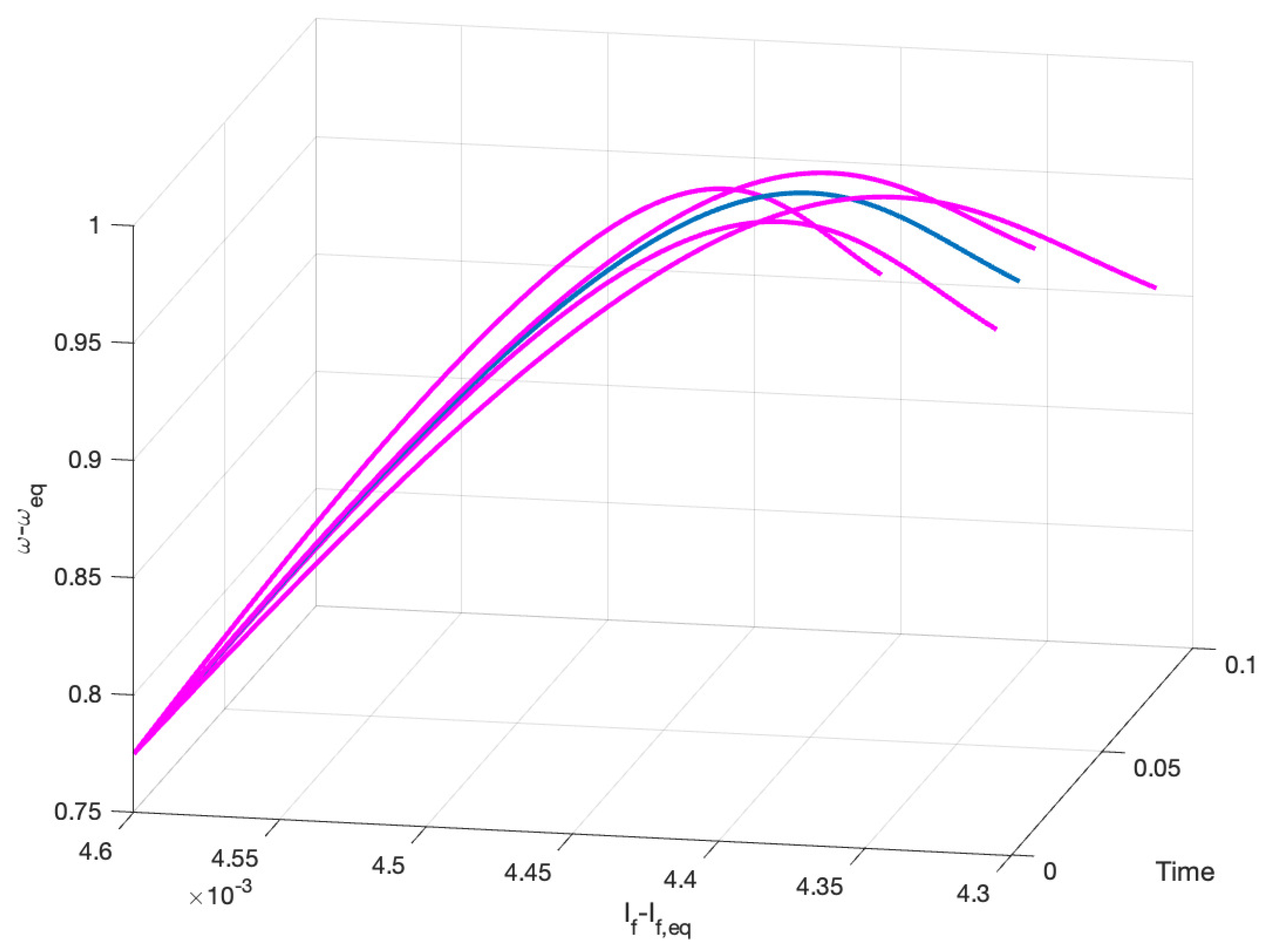
To empirically verify that the generated state tube entraps the nonlinear motor state trajector we have depicted in the following Figure 2 the unbiased time trend of the following 3D curve: ( t , I a ( t ) I a , r e f , ω ( t ) ω r e f ) , 0 t 0.1 , sec . This represents the free response of the motor (blue color curve, nonlinear model) and the four vertices (magenta color curves) depicting the boundaries of the state tube evolution that originates from a random unbiased initial state belonging to the box (31), (32). The choice of the third and fourth state variables is driven by the consideration that these state variables are the boxed ones; the voltage input has been kept constant to its reference value (0 in its unbiased version) since the actuator matrices G i are practically identical for each vertex.
Starting from the design knobs R x = diag 0 , 0 , 0 , 1 and R u = 0.1 , a sequence of 50 predecessor sets has been computed via recursions (13) and (14), and, for the sake of comparisons, the proposed Algorithm 1, based on the data-driven Algorithm 2, has been contrasted with a traditional model-based nonlinear MPC scheme NMPC [31]. The time horizon is 20 s and the motor initial state has been chosen as equal to x 0 = 100 , 20 , 0.1 , 50 T
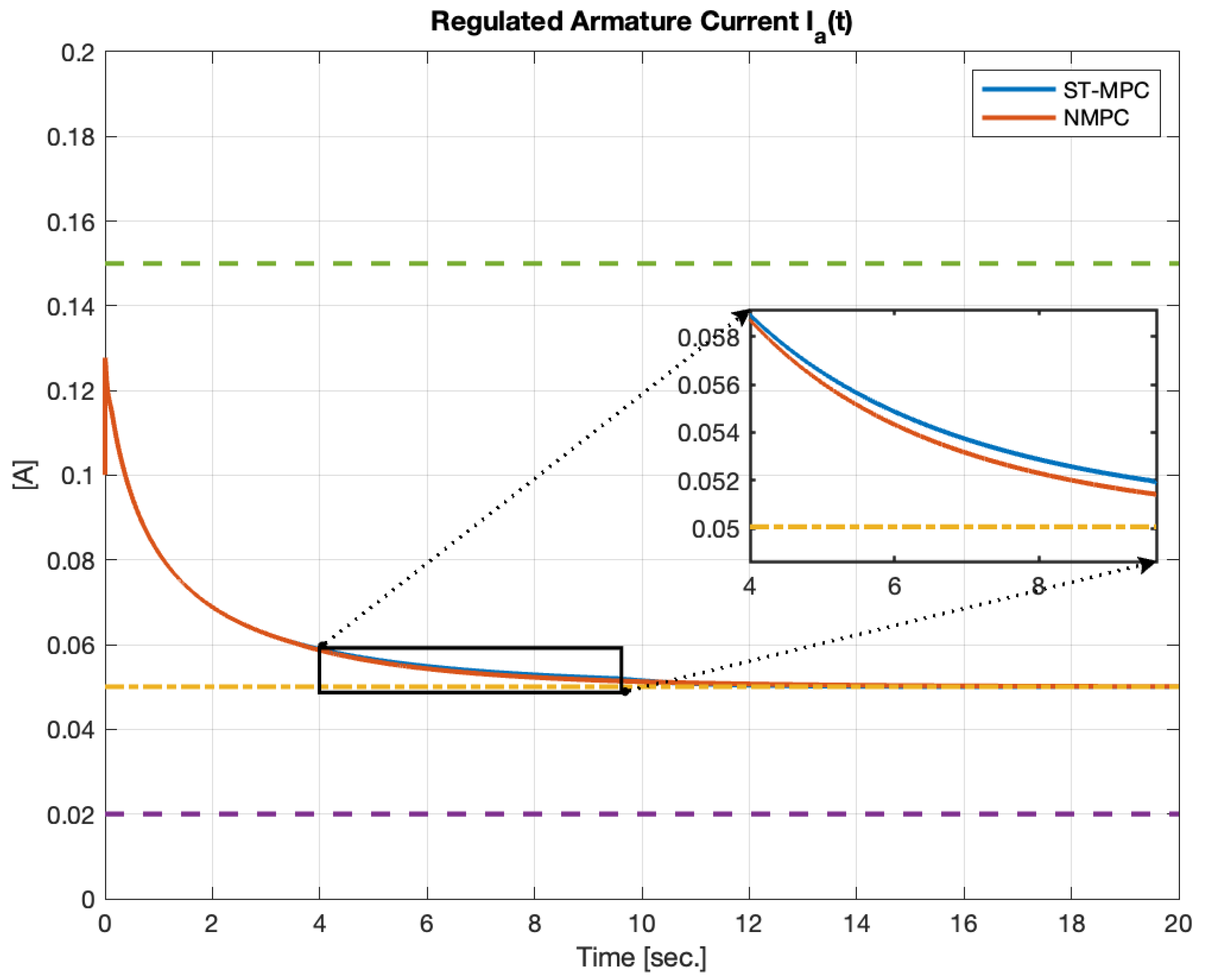
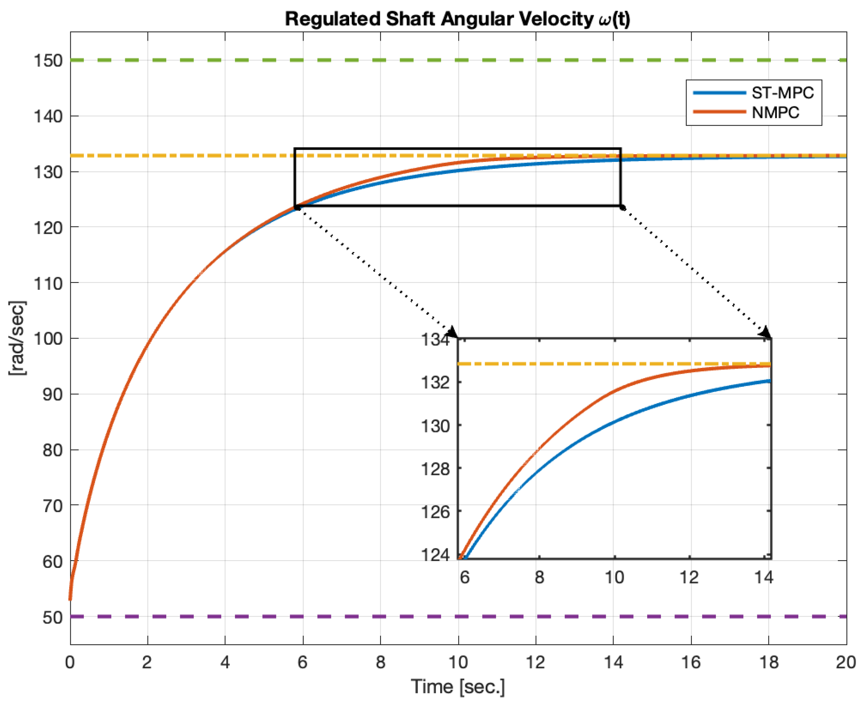
The on-line numerical results are collected in Figure 3, Figure 4 and Figure 5, where the boxed motor variables that regulate armature current, angular velocity, and voltage control input for the two strategies are depicted. The prescribed constraints are denoted by dashed horizontal lines, and the dash–dotted line represents the given equilibrium level. In order to understand how the regulated system behaves, let us start from Figure 4 (shaft angular velocity ω ( t ) and output target): the starting rotating regime, ω ( 0 ) = 50 rad sec , is below the desired target level ω r e f = 132.8373 rad sec (dash-dotted horizontal line), and as a consequence, the voltage control input V ( t ) (Figure 5) generates the highest possible voltage equal to 210 V , consistent with the imposed constraints (upper-level horizontal green dashed line in Figure 5), thus achieving an acceleration of the angular velocity towards the desired target. Whenever the angular velocity transient is near the end, the voltage control input starts decreasing towards the related equilibrium value (dash–dotted orange line in Figure 5). The armature current behavior I a ( t ) (Figure 3) complies with the voltage time trend, which is higher with regard to the equilibrium level during the initial time instants and then converges to the desired target value (dash–dotted orange line in Figure 3). In summary, all the prescribed constraints are satisfied at each time instant and the desired equilibrium levels are asymptotically reached. In Figure 3 and Figure 4, it can be noticed that the proposed Algorithm 1 and the NMPC competitor seem indistinguishable: to this end, the time trend of these variables have been properly zoomed (subplot graphs) with regard to a time window, the subset of the simulation horizon, to put into context how the two strategies differ. In particular, the difference between the proposed Algorithm 1 and the NMPC competitor can be can be understood by starting with Figure 5 (voltage control input): here, as expected, NMPC performs better (ad hoc scheme) by pushing the voltage level towards the upper saturation constraint (upper-level horizontal green dashed line in Figure 5) for a time interval longer than the proposed Algorithm 1. The NMPC’s better regulation of the performance with regard to the proposed Algorithm 1 is reflected on the regulated shaft angular velocity and armature current, even if it is slight; look at the zoomed subplots in Figure 3 and Figure 4 in terms of transient time trends. It must be noted that the two schemes have significantly different on-line computational complexities, as will be clear in the forthcoming analysis of the one-step-ahead controllable set T i time behavior.
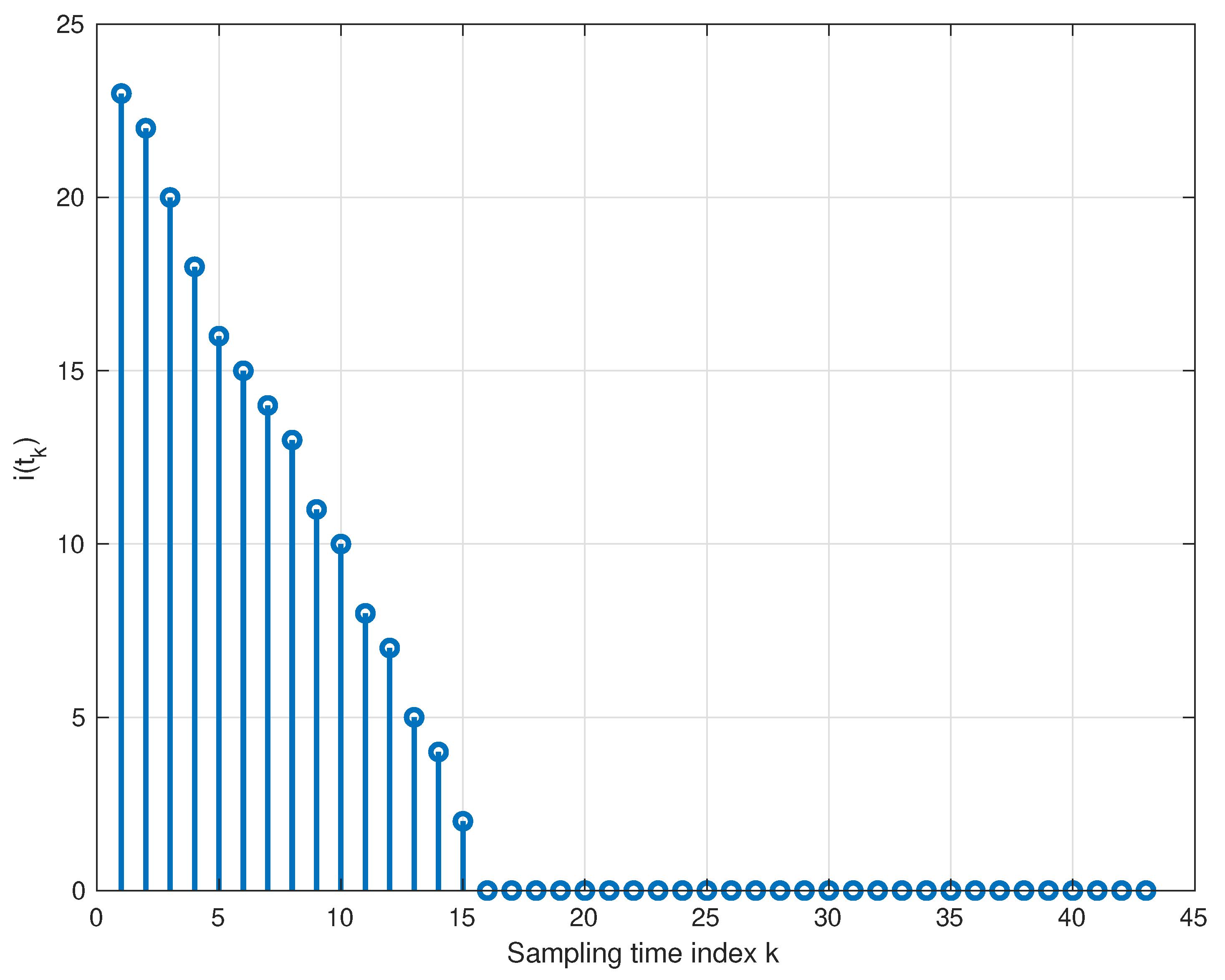
The switching signal taking care of the one-step state-ahead controllable sequence set membership level, showing that the regulated state trajectory converges in finite time (the first 45 sampling time steps and the initial state belongs to i ( t 0 ) = 23 ) to the RPI region E , is depicted in Figure 6. This figure represents nothing more than an experimental validation of the asymptotic stability of the regulated system in terms of Lyapunov arguments. The set-membership integer-valued function that decreases monotonically as the sampling step increases indicates in fact that the Lyapunov function, associated with the level curves generated from the shaping matrices of the one-step-ahead ellipsoidal sets T i ( k ) , also decreases monotonically along the trajectory of the regulated system. The figure has a direct interpretation regarding the computational burdens of the proposed Algorithm 1 strategy that requires solving a QP optimization problem for 15 consecutive sampling steps, starting from the initial time instant. From the next sampling step onwards, Algorithm 1 reduces to a linear-state feedback control law without any computational burden. The NMPC competing strategy, on the other hand, requires solving a QP optimization problem (in the best case) at every sampling step [31].
In summary, it can be noted for the DC motor (Example nr. 1) that the proposed Algorithm 1 strategy and the competitor NMPC perform similarly (but not identically) with respect to the depicted regulated state variables (Figure 3 and Figure 4). As expected, the competitor NMPC strategy outperforms the proposed Algorithm 1 in terms of voltage control time behavior (Figure 5). The two strategies differ significantly in terms of computational burdens: the proposed data-driven Algorithm 1 is preferable due to the practically negligible computational burden starting from a given finite time instant that is always guaranteed to exist (see [28] for details).

5.2. Continuous Stirred Tank Reactor

Consider the highly nonlinear model of a continuous stirred tank reactor (CSTR) [31]. Under the hypothesis of constant liquid volume, the CSTR for an exothermic, irreversible reaction A B is described by the following dynamic model based on a component balance for reactant A and an energy balance:
d C A d t = q V C A f C A ( t ) k 0 C A ( t ) e Δ E R T A ( t ) d T A d t = q V T f T A ( t ) + Δ H ρ C p k 0 e Δ E R T ( t ) C A ( t ) + + ρ c C p , c V ρ C p T c ( t ) ( 1 e H A ρ c C p , c T c ( t ) ) ( T c , 0 T A ( t ) )
where the following definitions apply:
  • C A ( t ) is the concentration of A in the reactor;
  • T A ( t ) is the reactor temperature;
  • T c ( t ) is the temperature of the coolant stream.
  • and the model parameters are q = 100 l min , V = 100 l , k 0 = 7.2 × 10 10 min 1 , T 0 = 350 K ; E R = 10 4 K ; ρ = ρ c = 1000 g l ; Δ H = 2 × 10 5 J mol , C p = C p , c = 1 J g K H A = 7 × 10 5 J min K , C A f = 1 J g K , T f = 350 K (see [38] for details on the meanings of these parameters). The resulting nonlinear model is then characterized by a two-state variable model in the form
d x d t = f ( x , u ) y ( t ) = C x ( t )
where x = C A , T A T (reactant concentration and temperature reaction), u = T c (coolant stream temperature, control signal) and the output is equal to the reactant concentration C A (as a consequence C = [ 1 0 ] ). Under the nominal operating condition, T c , e q = 97.6794 K ; the reactor exhibits an unstable but desirable equilibrium in terms of the reactant concentration value:
C A , e q , T A , e q T = 0.52 , 398.792 T
(the other two asymptotically stable equilibria do exist, but in terms of the reactant concentration value, they are of no interest). The sampling time has been chosen as equal to T s = 0.1 min , and the plant behavior has been discretized according to a forward-Euler scheme. The task consists of regulating the behavior of the reactant concentration around the desired equilibrium value by acting on the coolant stream temperature T c under the action of initial state conditions acting as perturbations with regard to to the normal operating condition. An MPC strategy will be designed under the hypothesis that the state and input variables belong to the following constraints box:
0.3 C A ( t ) 0.6
395 T A ( t ) 405
80 T c ( t ) 120
A possible interpretation of the previous box could be in terms of reactor safety. According to Section 4 prescriptions, a polytopic embedding of the nonlinear plant (28) inside the box (36)–(38) has been derived off-line by applying the Algorithm 2. To this end, r = 50 equilibria have been exploited by means of a gridding selection procedure to achieve a multi-model description (26), compatible with N s = 10 8 data sequences { u s , x s i ( t ) } generated by the Monte Carlo simulation unit. The resulting matrix vertices are
Φ 1 = 2.3682 0.1303 1.4524 1.0461 , G 1 = 5 e 4 4.9 e 2
Φ 2 = 2.5693 0.0415 0.8275 0.8936 , G 2 = 5 e 4 4.6 e 2
Φ 3 = 2.1213 0.2886 2.4767 1.4602 , G 3 = 4.5 e 4 4.3 e 2
Φ 4 = 3.1508 0.5255 1.0670 0.6757 , G 4 = 4.5 e 4 4.1 e 2
Φ 5 = 2.7036 0.1576 1.1885 0.8158 , G 5 = 5 e 4 5.6 e 2
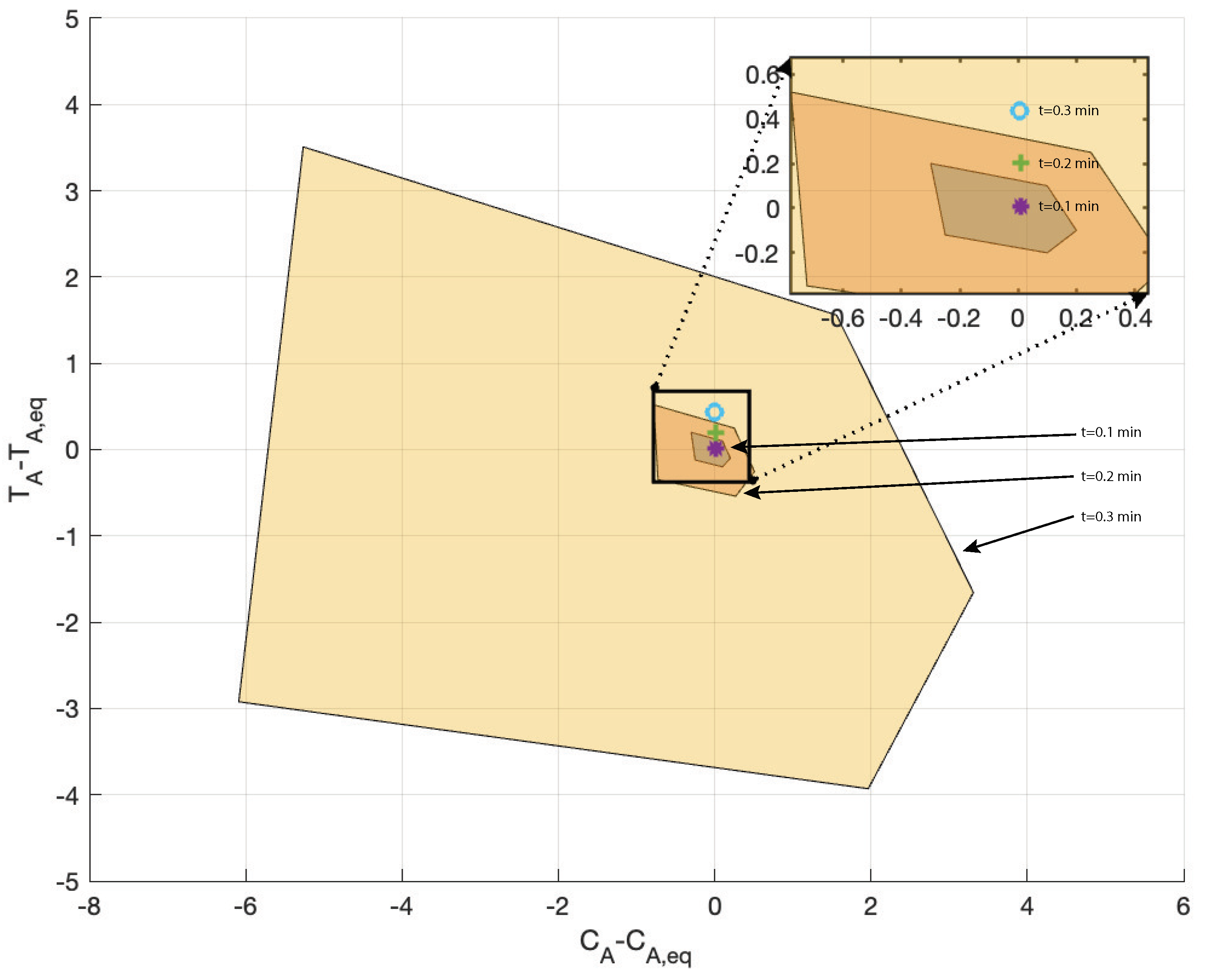
To empirically verify that the generated state tube entraps the nonlinear motor state trajectory, we face a situation that is different with regard to the previous example since the equilibrium is unstable and the obtained polytope LTI vertices are unstable too. As a consequence, it is not possible to depict the state trajectory tube using a 3D representation since the tube sides are numerically diverging at a fast rate. To overcome this practical drawback and by considering that the system has a planar state, we have depicted in the following Figure 7 the free response time evolution on the plane C A C A , e q . T A T A , e q of an outer approximation of the state tube for three sampling instants, t = 0.1 , 0.2 , and 0.3 min (a photo-shoot-like image). The polygonal figure vertices are vectors aligned along the direction of the unstable eigenvectors of the polytope LTI matrices Φ i , i = 1 , 2 , 3 , 4 , 5 . The bullet points are the sampled values of the unbiased free-state evolution CSTR discretized nonlinear model for t = 0.1 min (asterisk), t = 0.2 min (cross), and t = 0.3 min (bullet). It can be noticed that all the three points belong to the respective polygonal region.
Starting from the design knobs R x = diag 1 , 0 and R u = 0.01 , a sequence of 30 predecessor sets has been computed via recursions (13), and (14) and, similarly to the previous experiment, the proposed Algorithm 1 scheme has been compared with the NMPC competitor. The time horizon is 10 min and the CSTR initial state has been chosen as equal to x 0 = 0.3 , 402 T ; notice that for this particular choice, the concentration initial value has been chosen as equal to the left boundary of the admissible region (36).
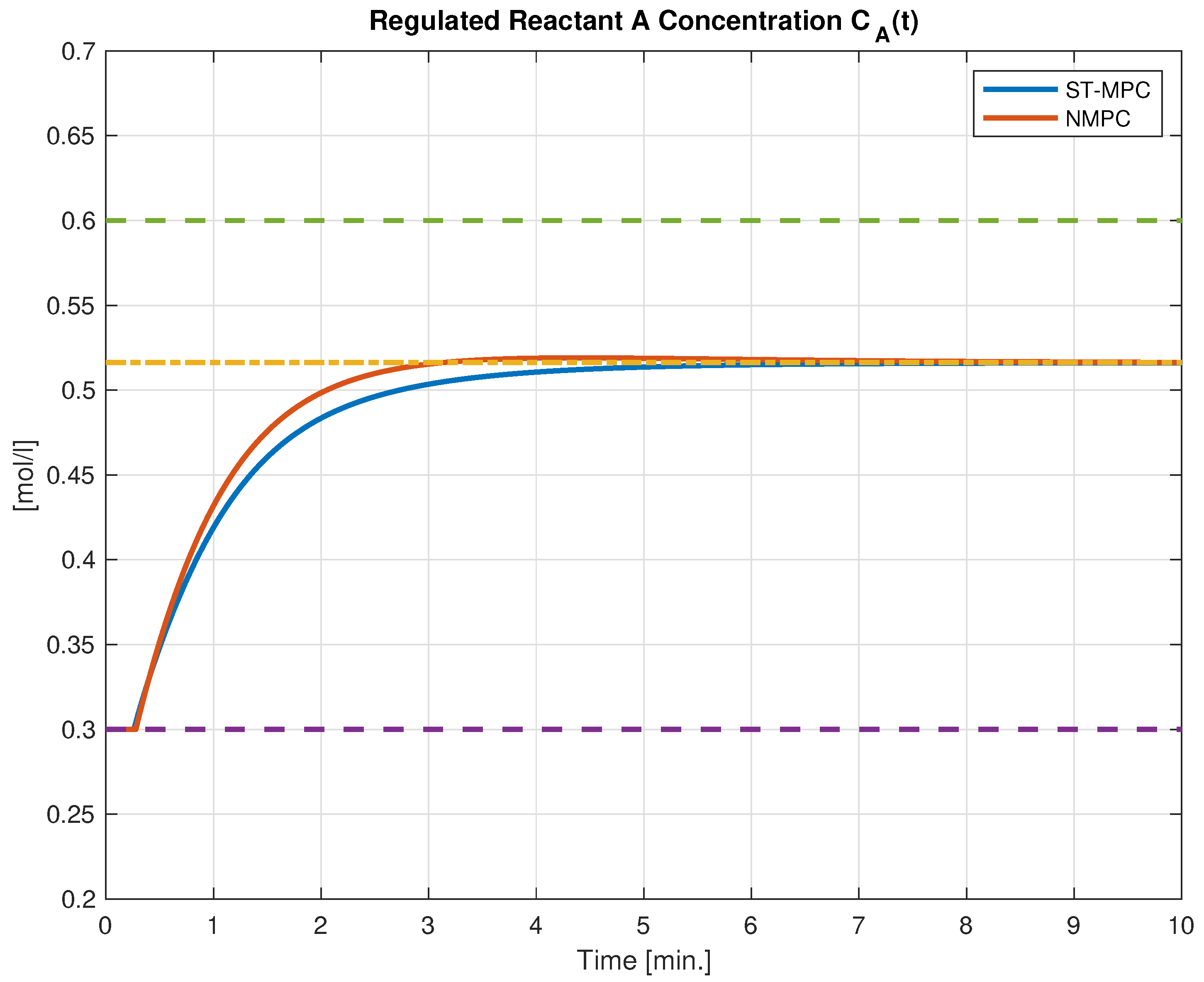
The on-line numerical results are collected in Figure 8, Figure 9 and Figure 10, where the boxed CSTR variables of concentration C A ( t ) , reactor temperature T A ( t ) , and coolant stream temperature (control input) T c ( t ) for the two strategies are depicted. The prescribed constraints are denoted by dashed horizontal lines, and the dash–dotted line represents the given equilibrium level. All the prescribed constraints are satisfied at each time instant, and the desired equilibrium levels are asymptotically reached. Unlike the previous example, it can be noticed that the proposed Algorithm 1 and the NMPC are no longer indistinguishable and it can be noticed that, for all the time trends, the NMPC regulated state variables (as expected) are performing better than the proposed Algorithm 1 competitor. In addition, it can be also noted, thanks to the particular choice of the initial state that both strategies, Algorithm 1, which was proposed, and NMPC, which is the competitor, saturate their state values on the initial time instants of the C A ( t ) graphical depiction (Figure 8). Similarly to the previous example, in order to have a regulated system behavior comprehension, let us start from Figure 8 (Reactant A concentration C A ( t ) and output target): the initial value, C A ( 0 ) = 0.3 J g K , is below the desired Reactant A concentration target level C A , r e f = 0.52 J g K (dash–dotted horizontal line), and the initial reactor temperature value T A ( 0 ) = 402 K is above the corresponding equilibrium target value T A , r e f = 398.792 K ; as a consequence, the coolant stream temperature control signal T c ( t ) (Figure 10) must jointly cool down the reactor temperature to increase the reactant concentration. This is achieved via the MPC strategy which changes the coolant stream temperature to the lowest possible level, 80 K , consistent with the imposed constraints (lower-level horizontal magenta dashed line in Figure 10), so that, as previously stated, the reactor chamber will jointly achieve an increase in the reactant production (measured by the C A ( t ) quantity) and a decrease in the reaction temperature T A ( t ) . Whenever, for both state variables, C A ( t ) and T A ( t ) , the transient is near the end, the coolant stream temperature input increases towards the related equilibrium value (dash–dotted orange line in Figure 10) and the reaction then reaches its steady-state behavior. The difference between the proposed Algorithm 1 and the NMPC competitor can be can be understood by jointly analyzing the temperature trends shown in Figure 10 (coolant stream control input) and Figure 9 (reactor temperature): here, the NMPC cooling down phenomenon is more rapid with regard to the corresponding proposed Algorithm 1 behavior. A possible explanation consists of the NMPC algorithm having a better understanding of the reactor model (ad hoc model-based scheme). This leads to a faster convergence of the controlled variables towards the desired equilibrium, while also ensuring better safety conditions (fewer undershoot phenomena in the reactor temperature time trend T A ( t ) , Figure 9). The two schemes have significant different on-line computational complexities, as will be clear in the forthcoming analysis.
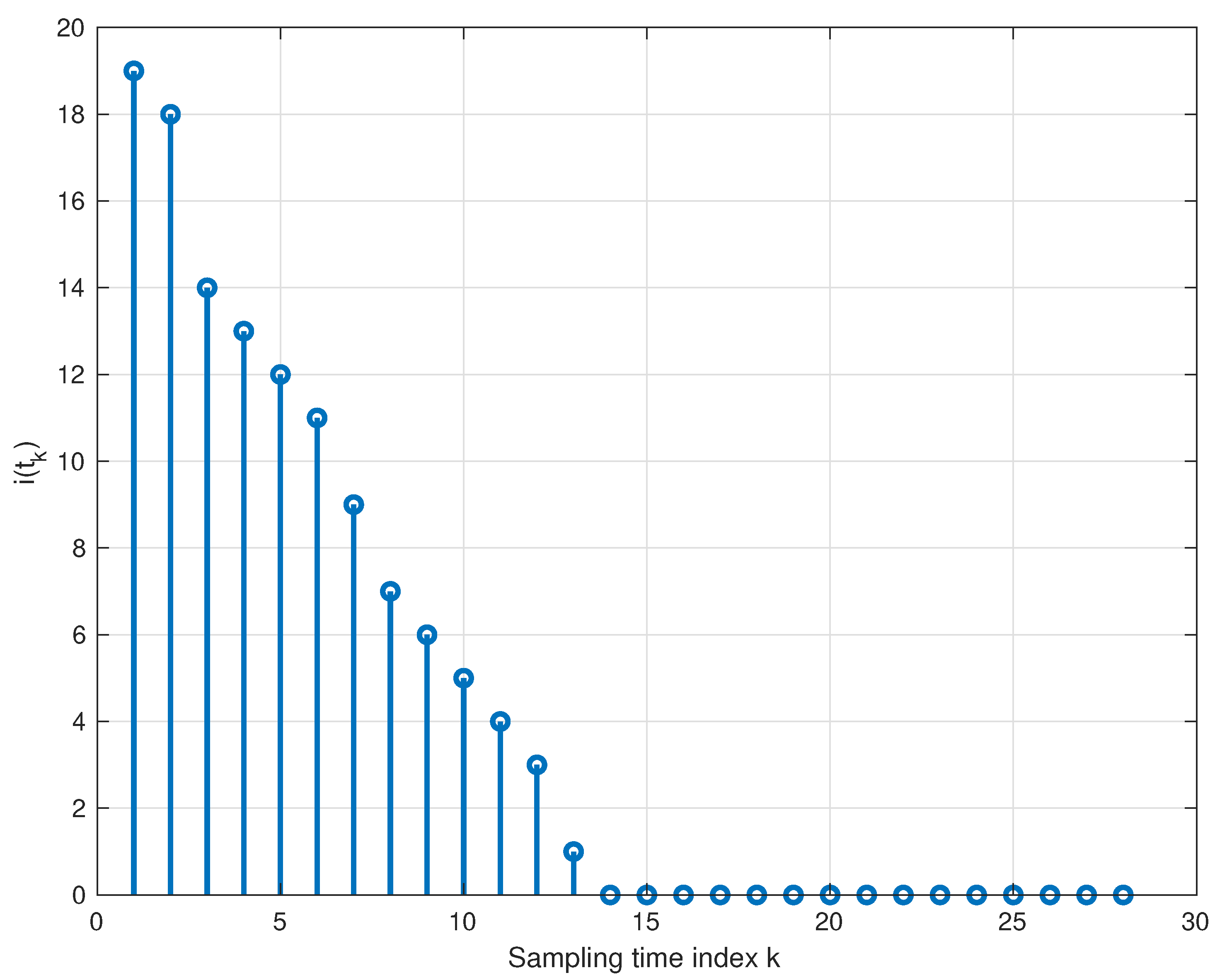
The Lyapunov-like switching signal takes care of the one-step state-ahead controllable sequence set-membership level, showing that the regulated state trajectory converges in finite time (the first 29 sampling time steps and the initial state belongs to i ( t 0 ) = 19 ) to the RPI region E , which is depicted in Figure 11. In this case, the Algorithm 1 strategy requires solving a QP optimization problem for 13 consecutive sampling steps, starting from the initial time instant. Similar considerations to the previous example can be made regarding the choice of the proposed data-driven Algorithm 1 controller compared to its competitor.

5.3. Computational Burdens

The common denominator between the two proposed examples is represented by the computational burdens of the data-driven Algorithm 1 that is allocated mainly in the off-line phase (performed off-line before plant operations). As for the on-line phase, the numerical effort is related to the set-membership level signal i ( t k ) :
  • When i ( t k ) = 0 , it results in a trivial matrix-vector multiplication;
  • When i ( t k ) 0 , it requires the solution of a quadratic programming problem (QP) with linear constraints whose computational complexity is O ( ν 3 ) ( ν is the optimization problem dimension size) [39].
Since the proposed strategy is capable of driving the regulated plant state in a finite number of steps (at most N, where N is the number of the E i sets) to the RPI region E 0 [28], the proposed Algorithm 1 is required to solve a QP procedure only for a finite number of times. The NMPC strategy conversely requires, for each step, the solution of a quadratic program (QP) or Second-Order Cone Program (SOCP) ( O ( ν 3 ) in the best-case scenario) [40].

6. Conclusions and Future Studies

This paper presents an innovative data-driven set-theoretic receding horizon control (RHC) algorithm specifically designed for constrained single-input single-output (SISO) nonlinear systems. By analyzing input/output data sequences, the algorithm demonstrates its ability to compute a polytopic outer embedding of the nonlinear plant using the proposed iterative machine learning approach.
In terms of future development, several key areas will be prioritized to enhance the algorithm’s capabilities and robustness. First, methodological refinements will be undertaken to extend the algorithm’s applicability to a broader range of nonlinear systems, including multi-input multi-output (MIMO) configurations and systems with non stationary dynamic characteristics (drifting parameters, time-varying targets etc.).
Secondly, it is crucial to decouple the RHC design from explicit state model descriptions. This involves developing model-agnostic approaches that can maintain performance without relying on detailed state-space representations, thereby increasing the flexibility and adaptability of the control strategy.
Lastly, the real-time adaptability and effectiveness of these learning-based controllers will be rigorously assessed. This includes implementing the algorithm in real-world scenarios to evaluate its performance under different operating conditions and disturbances. Additionally, strategies to reduce computational overhead and improve the algorithm’s response time will be explored, ensuring its practical viability for real-time applications.
Overall, these advancements will significantly contribute to the development of more versatile, efficient, and reliable data-driven RHC algorithms for nonlinear control systems.

Author Contributions

Conceptualization, F.G.; Methodology, D.F.; Software, D.F. All authors have read and agreed to the published version of the manuscript.

Funding

This research received no external funding.

Data Availability Statement

The original contributions presented in the study are included in the article, further inquiries can be directed to the corresponding author.

Conflicts of Interest

The authors declare no conflict of interest.

References

  1. Rawlings, J.; Mayne, D.; Diehl, M. Model Predictive Control: Theory, Computation, and Design; Nob Hill Publishing: London, UK, 2017. [Google Scholar]
  2. Hou, Z.S.; Wang, Z. From model-based control to data-driven control: Survey, classification and perspective. Inf. Sci. 2013, 235, 3–35. [Google Scholar] [CrossRef]
  3. van Waarde, H.J.; Eising, J.; Trentelman, H.L.; Camlibel, M.K. Data Informativity: A New Perspective on Data-Driven Analysis and Control. IEEE Trans. Autom. Control 2020, 65, 4753–4768. [Google Scholar] [CrossRef]
  4. Dörfler, F.; Coulson, J.; Markovsky, I. Bridging Direct and Indirect Data-Driven Control Formulations via Regularizations and Relaxations. IEEE Trans. Autom. Control 2023, 68, 883–897. [Google Scholar] [CrossRef]
  5. Krishnan, V.; Pasqualetti, F. On Direct vs. Indirect Data-Driven Predictive Control. In Proceedings of the 2021 60th IEEE Conference on Decision and Control (CDC), Austin, TX, USA, 14–17 December 2021; pp. 736–741. [Google Scholar] [CrossRef]
  6. Verheijen, P.; Breschi, V.; Lazar, M. Handbook of linear data-driven predictive control: Theory, implementation and design. Annu. Rev. Control 2023, 56, 100914. [Google Scholar] [CrossRef]
  7. Formentin, S.; van Heusden, K.; Karimi, A. Model-based and data-driven model-reference control: A comparative analysis. In Proceedings of the 2013 European Control Conference (ECC), Zurich, Switzerland, 17–19 July 2013; pp. 1410–1415. [Google Scholar] [CrossRef]
  8. Xie, W.; Bonis, I.; Theodoropoulos, C. Data-driven model reduction-based nonlinear MPC for large-scale distributed parameter systems. J. Process. Control 2015, 35, 50–58. [Google Scholar] [CrossRef]
  9. Han, H.; Liu, Z.; Liu, H.; Qiao, J. Knowledge-Data-Driven Model Predictive Control for a Class of Nonlinear Systems. IEEE Trans. Syst. Man, Cybern. Syst. 2021, 51, 4492–4504. [Google Scholar] [CrossRef]
  10. Stoffel, P.; Berktold, M.; Müller, D. Real-life data-driven model predictive control for building energy systems comparing different machine learning models. Energy Build. 2024, 305, 113895. [Google Scholar] [CrossRef]
  11. Kim, H.; Nair, S.H.; Borrelli, F. Scalable Multi-modal Model Predictive Control via Duality-based Interaction Predictions. arXiv 2024, arXiv:cs.RO/2402.01116. [Google Scholar]
  12. Vinod, D.; Singh, D.; Saikrishna, P.S. Data-Driven MPC for a Fog-Cloud Platform with AI-Inferencing in Mobile-Robotics. IEEE Access 2023, 11, 99589–99606. [Google Scholar] [CrossRef]
  13. Shah, K.; He, A.; Wang, Z.; Du, X.; Jin, X. Data-Driven Model Predictive Control for Roll-to-Roll Process Register Error. In Proceedings of the 2022 International Additive Manufacturing Conference, International Manufacturing Science and Engineering Conference, Lisbon, Portugal, 19–20 October 2022; p. V001T03A006. [Google Scholar] [CrossRef]
  14. Baby, T.V.; Sotoudeh, S.M.; HomChaudhuri, B. Data-Driven Prediction and Predictive Control Methods for Eco-Driving in Production Vehicles. IFAC-PapersOnLine 2022, 55, 633–638. [Google Scholar] [CrossRef]
  15. Brunton, S.L.; Proctor, J.L.; Kutz, J.N. Discovering governing equations from data by sparse identification of nonlinear dynamical systems. Proc. Natl. Acad. Sci. USA 2016, 113, 3932–3937. [Google Scholar] [CrossRef]
  16. Prag, K.; Woolway, M.; Celik, T. Toward Data-Driven Optimal Control: A Systematic Review of the Landscape. IEEE Access 2022, 10, 32190–32212. [Google Scholar] [CrossRef]
  17. Alsalti, M.; Lopez, V.G.; Berberich, J.; Allgöwer, F.; Müller, M.A. Data-driven nonlinear predictive control for feedback linearizable systems. IFAC-PapersOnLine 2023, 56, 617–624. [Google Scholar] [CrossRef]
  18. Sawant, S.; Reinhardt, D.; Kordabad, A.B.; Gros, S. Model-Free Data-Driven Predictive Control Using Reinforcement Learning. In Proceedings of the 2023 62nd IEEE Conference on Decision and Control (CDC), Marina Bay Sands, Singapore, 13–15 December 2023; pp. 4046–4052. [Google Scholar] [CrossRef]
  19. Zhou, Y.; Li, D.; Xi, Y.; Gan, Z. Synthesis of model predictive control based on data-driven learning. Sci. China Inf. Sci. 2019, 63, 189204. [Google Scholar] [CrossRef]
  20. Fortino, G.; Savaglio, C.; Spezzano, G.; Zhou, M. Internet of Things as System of Systems: A Review of Methodologies, Frameworks, Platforms, and Tools. IEEE Trans. Syst. Man, Cybern. Syst. 2021, 51, 223–236. [Google Scholar] [CrossRef]
  21. Belhadi, A.; Djenouri, Y.; Srivastava, G.; Djenouri, D.; Lin, J.C.W.; Fortino, G. Deep learning for pedestrian collective behavior analysis in smart cities: A model of group trajectory outlier detection. Inf. Fusion 2021, 65, 13–20. [Google Scholar] [CrossRef]
  22. Coulson, J.; Lygeros, J.; Dörfler, F. Data-Enabled Predictive Control: In the Shallows of the DeePC. In Proceedings of the 2019 18th European Control Conference (ECC), Naples, Italy, 25–28 June 2019; pp. 307–312. [Google Scholar] [CrossRef]
  23. Bongard, J.; Berberich, J.; Köhler, J.; Allgöwer, F. Robust Stability Analysis of a Simple Data-Driven Model Predictive Control Approach. IEEE Trans. Autom. Control 2023, 68, 2625–2637. [Google Scholar] [CrossRef]
  24. Willems, J.C.; Rapisarda, P.; Markovsky, I.; De Moor, B.L. A note on persistency of excitation. Syst. Control Lett. 2005, 54, 325–329. [Google Scholar] [CrossRef]
  25. De Persis, C.; Tesi, P. Formulas for Data-Driven Control: Stabilization, Optimality, and Robustness. IEEE Trans. Autom. Control 2020, 65, 909–924. [Google Scholar] [CrossRef]
  26. Markovsky, I. Data-Driven Simulation of Generalized Bilinear Systems via Linear Time-Invariant Embedding. IEEE Trans. Autom. Control 2023, 68, 1101–1106. [Google Scholar] [CrossRef]
  27. Giannini, F.; Franzè, G.; Pupo, F.; Fortino, G. Set-theoretic receding horizon control for nonlinear systems: A data-driven approach. In Proceedings of the IEEE EUROCON 2023—20th International Conference on Smart Technologies, Torino, Italy, 6–8 July 2023; pp. 579–584. [Google Scholar] [CrossRef]
  28. Angeli, D.; Casavola, A.; Franzè, G.; Mosca, E. An ellipsoidal off-line MPC scheme for uncertain polytopic discrete-time systems. Automatica 2008, 44, 3113–3119. [Google Scholar] [CrossRef]
  29. Angeli, D.; Casavola, A.; Mosca, E. Constrained predictive control of nonlinear plants via polytopic linear system embedding. Int. J. Robust Nonlinear Control 2000, 10, 1091–1103. [Google Scholar] [CrossRef]
  30. Boyd, S.; El Ghaoui, L.; Feron, E.; Balakrishnan, V. Linear Matrix Inequalities in System and Control Theory; SIAM Studies in Applied Mathematics: Philadelphia, PA, USA, 1994; p. 15. [Google Scholar]
  31. Magni, L.; De Nicolao, G.; Scattolini, R.; Allgöwer, F. Robust model predictive control for nonlinear discrete-time systems. Int. J. Robust Nonlinear Control 2003, 13, 229–246. [Google Scholar] [CrossRef]
  32. Blanchini, F.; Miani, S. Set-Theoretic Methods in Control, 1st ed.; Birkhäuser: Basel, Switzerland, 2007. [Google Scholar]
  33. Kurzhanski, A.; Valyi, I. Ellipsoidal Calculus for Estimation and Control; Systems & Control: Foundations & Applications; Birkhäuser: Boston, MA, USA, 1996. [Google Scholar]
  34. Kočvara, M.; Stingl, M. PENNON: A code for convex nonlinear and semidefinite programming. Optim. Methods Softw. 2003, 18, 317–333. [Google Scholar] [CrossRef]
  35. Russell, S.; Norvig, P. Artificial Intelligence: A Modern Approach, 3rd ed.; Prentice Hall Press: Englewood Cliffs, NJ, USA, 2009. [Google Scholar]
  36. Jampani, R.; Xu, F.; Wu, M.; Perez, L.L.; Jermaine, C.; Haas, P.J. MCDB: A monte carlo approach to managing uncertain data. In Proceedings of the SIGMOD ’08 2008 ACM SIGMOD International Conference on Management of Data, New York, NY, USA, 9–12 June 2008; pp. 687–700. [Google Scholar] [CrossRef]
  37. Krause, P.; Wasynczuk, O.; Sudhoff, S.; Pekarek, S. Analysis of Electric Machinery and Drive Systems; IEEE Press Series on Power and Energy Systems; Wiley: Hoboken, NJ, USA, 2013. [Google Scholar]
  38. Pipino, H.A.; Cappelletti, C.A.; Adam, E.J. Adaptive multi-model predictive control applied to continuous stirred tank reactor. Comput. Chem. Eng. 2021, 145, 107195. [Google Scholar] [CrossRef]
  39. Ben-Tal, A.; Nemirovski, A. Lectures on Modern Convex Optimization; Society for Industrial and Applied Mathematics: Philadelphia, PA, USA, 2001. [Google Scholar] [CrossRef]
  40. Cannon, M. Efficient nonlinear model predictive control algorithms. Annu. Rev. Control 2004, 28, 229–237. [Google Scholar] [CrossRef]
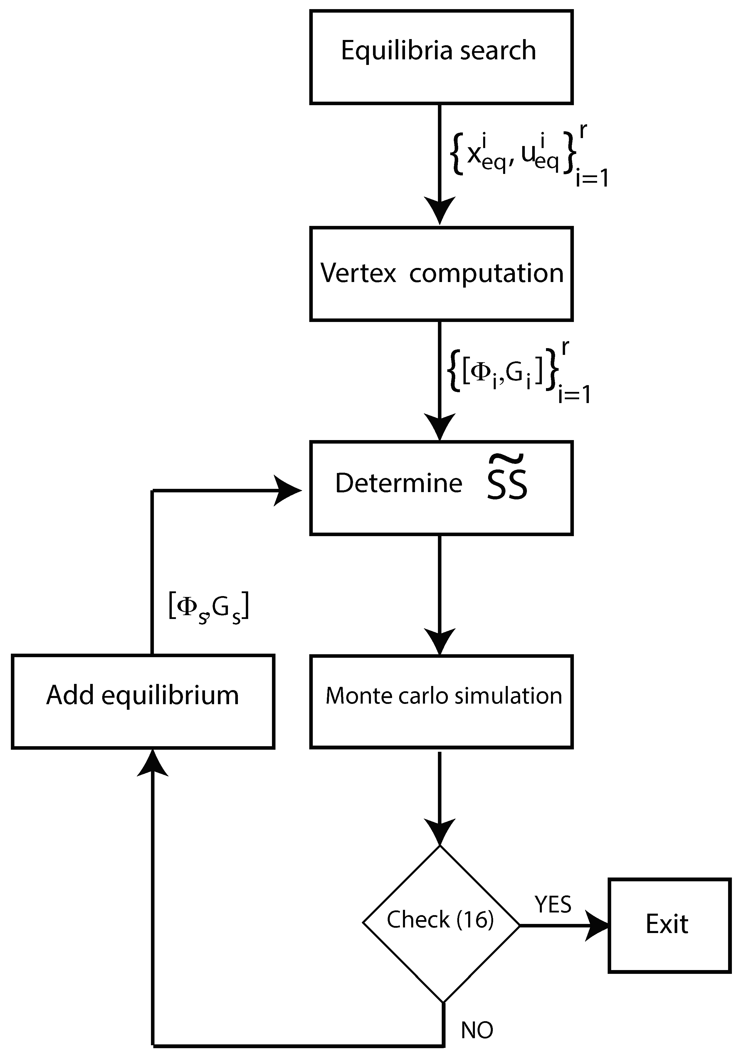
Figure 1. Iterative machine learning algorithm: the flowchart.
Information 15 00369 g001
Figure 2. ( t , I a ( t ) I a , r e f , ω ( t ) ω r e f ) , 0 t 0.1 , sec . free evolution. Motor nonlinear model time trend (blue line), linear vertices time trend (magenta lines).
Information 15 00369 g002
Figure 3. Armature current-regulated time trend: Algorithm 1 strategy (blue line) and NMPC strategy (red line), prescribed constraints (dashed horizontal lines), and equilibrium level (dash–dotted line).
Information 15 00369 g003
Figure 4. Angular velocity-regulated time trend: Algorithm 1 strategy (blue line) and NMPC strategy (red line), prescribed constraints (dashed horizontal lines), and equilibrium level (dash–dotted line).
Information 15 00369 g004
Figure 5. Voltage control input time trend: Algorithm 1 strategy (blue line) and NMPC strategy (red line), prescribed constraints (dashed horizontal lines), and equilibrium level (dash–dotted line).
Information 15 00369 g005
Figure 6. Algorithm 1 strategy set-membership level signal (DC motor example).
Information 15 00369 g006
Figure 7. Free response state tube outer approximation (polygonal regions) planar depiction in the plane C A C A , e q , T A T A , e q , for t = 0.1 , 0.2 , and 0.3 min (free evolution). The bullet points are representing the nonlinear CSTR free response, evaluated at t = 0.1 min (asterisk), t = 0.2 min (cross), and t = 0.3 min (bullet).
Information 15 00369 g007
Figure 8. Reactant A concentration C A ( t ) regulated time trend: Algorithm 1 strategy (blue line) and NMPC strategy (red line), prescribed constraints (dashed horizontal lines), equilibrium level (dash–dotted line).
Information 15 00369 g008
Figure 9. Reactor temperature T A ( t ) regulated time trend: Algorithm 1 strategy (blue line) and NMPC strategy (red line), prescribed constraints (dashed horizontal lines), equilibrium level (dash–dotted line).
Information 15 00369 g009
Figure 10. Coolant stream (control input) T c ( t ) regulated time trend: Algorithm 1 strategy (blue line) and NMPC strategy (red line), prescribed constraints (dashed horizontal lines), equilibrium level (dash–dotted line).
Information 15 00369 g010
Figure 11. Algorithm 1 strategy set-membership level signal (CSTR example).
Information 15 00369 g011
Disclaimer/Publisher’s Note: The statements, opinions and data contained in all publications are solely those of the individual author(s) and contributor(s) and not of MDPI and/or the editor(s). MDPI and/or the editor(s) disclaim responsibility for any injury to people or property resulting from any ideas, methods, instructions or products referred to in the content.