Exploring the Depths of the Autocorrelation Function: Its Departure from Normality

Abstract

In this article, we study the autocorrelation function (ACF), which is a crucial element in time series analysis. We compare the distribution of the ACF, both from a theoretical and empirical point of view. We focus on white noise processes (WN), i.e., uncorrelated, centered, and identically distributed variables, whose ACFs are supposed to be asymptotically independent and converge towards the same normal distribution. But, the study of the sum of the sample ACF contradicts this property. Thus, our findings reveal a deviation of the sample ACF from normality beyond a specific lag. Note that this phenomenon is observed for white noise of varying lengths, and evenforn the residuals of an ARMA($p,q$) model. This discovery challenges traditional assumptions of normality in time series modeling. Indeed, when modeling a time series, the crucial step is to validate the estimated model by checking that the associated residuals form white noise. In this study, we show that the widely used portmanteau tests are not completely accurate. Box–Pierce appears to be too conservative, whereas Ljung–Box is too liberal. We suggest an alternative method based on the ACF for establishing the reliability of the portmanteau test and the validity of the estimated model. We illustrate our methodology using money stock data in the USA.

1. Introduction

Time series data, characterized by their sequential nature, appear in many application domains, ranging from economics [1,2,3,4,5] and finance [6] or medicine [7,8,9] to climate modeling [10,11]. In this field, understanding and extracting meaningful information from data depends on our ability to manage their inherent temporal dependencies. The autocorrelation function (ACF) appears to be essential for this purpose [12,13,14,15,16,17,18,19,20,21,22,23]. Indeed, the ACF is a statistical measure that quantifies the relationship between a time series and its lagged versions at different time intervals.

For successive uncorrelated observations, such as a white noise (WN), the ACF is zero, and for observations that are no longer correlated if their lag-difference is larger than q, as it is the case in moving average models, called MA(q), then ACF cancels after lag q. Thus, the ACF can be used to identify these underlying models. But, the importance of ACF in time series modeling goes beyond the identification of white noise or MA(q) processes. It can also detect non-stationary components that structure the series, such as trends [24,25,26] or cyclical behavior [27]. Moreover ACFs are also useful to detect a long memory behavior [28,29,30]. And, last but not least, ACF plays a crucial role in time series modeling, since the validation of the estimated model depends on the study of its residuals, which is achieved thanks to their ACF. Knowledge of the empirical ACF distribution is therefore the basis for statistical inference in time series analysis. Indeed, the decision rules used in practice when modeling time series are based on the expected behavior of ACFs under different models [13,14].

In this paper, we focus on white noise processes whose ACFs are supposed to be asymptotically independent and to converge towards the same normal distribution. But, the study of the sum of the sample ACF contradicts this property. Indeed, whatever the observed time series, the sum of all the sample ACFs is a constant, equal to $-{\displaystyle \frac{1}{2}}$ [17]. Numerous research studies have underscored the significance of Hassani’s $-{\displaystyle \frac{1}{2}}$ theorem for practical applications and its integration into time series analysis and model development [31,32,33,34]. The implications of this remarkable consistency are profound, particularly for the fields of time series model building and analysis [35,36,37]. For a selected recent work highlighting the importance of considering the sample ACF in analysis, especially in the context of Hassani’s $-{\displaystyle \frac{1}{2}}$ theorem, see [38,39,40].

In this paper, we explore the theoretical and empirical properties of ACF and its cumulative sums (SACF). Our objective is to highlight the disparities that exist between the theoretical expectations and the empirical realities of these statistical measures. Our findings reveal a deviation of the sample ACF from normality beyond a specific lag. Note that this phenomenon is observed for white noise of varying lengths, with WN that are either Gaussian or not. Moreover, even the residuals of an ARMA($p,q$) model show the same behavior. This discovery challenges traditional assumptions of ACF normality in time series modeling. Indeed, when modeling a time series, the crucial step is to validate the estimated model by checking that the associated residuals form white noise, which is achieved by applying a portmanteau test (Box–Pierce or Ljung–Box tests), which is based on the independence and standard normality of the ACF [12,19].

Then, this study opens the way for re-evaluating and refining existing methodologies, in particular the widely used Box–Pierce and Ljung–Box tests. We employ both simulated data and real-world time series data to validate and emphasize the practical relevance of the results obtained of our study. We aim to contribute valuable insights that enhance the understanding and application of ACF in the field of time series analysis.

The paper is organized as follows. In Section 2, we describe the methods usually used to model time series. Within this section, we define the autocorrelation function, both theoretical and empirical; we explain the asymptotic behavior of its estimators in a WN framework and its theoretical implication for the SACF; and we recall the widely used portmanteau tests. In Section 4, we recall Hassani’s $-{\displaystyle \frac{1}{2}}$ theorem and derive contradictions with the previous results given in Section 2, with questions for the normality of the sample ACFs themselves. In Section 5, we simulate WN, either Gaussian or exponential, and we analyze the normality of both their ACF and SACFas a function of the series length and number of simulations. Normality is tested using the Shapiro test, and the Kolmogorov–Smirnov test is used when the theoretical distribution can be specified. The deviation from normality is highlighted mainly because of the flagrant non-normality of the SACFs. We also adopt a point of view that is consistent with practical analyses, since we additionally test the fit of successive ACFs with the Gaussian $\mathcal{N}\left(0,{\displaystyle \frac{1}{n}}\right)$ distribution, where n is the length of the series under consideration. This property is the basis of portmanteau tests and must be verified. Since the reliability of the portmanteau tests appears to be related to the good normality properties of the successive SACF and ACF, it seems important to check them on the residuals of the estimated model before applying the portmanteau validation tests. In Section 6, we simulate ARIMA(0,2,2) processes and estimate the simulated series using a more restrictive model—that is, an ARIMA(0,2,0)—to highlight the effects of mis-specifying parameter q. We illustrate this procedure in the last section using a real dataset: money stock data in USA.

Finally, in a Supplementary File, we consider WN with a shorter length n and the residuals of more complex ARIMA($p,d,q$) processes. We simulate ARIMA($p,d,q$) processes, estimate these simulations, and study their residuals. We distinguish the case where the orders $p^{\prime },d^{\prime },q^{\prime }$ of the estimated model are well-specified (equal to the convenient $p,d,q$ parameters used for simulations) from the case where they are not. For these residuals of the simulations, we repeat the analyses introduced in Section 5. When the model is well-specified or mis-specified, but with a more general model ($p^{\prime }\ge p,d^{\prime }\ge d,q^{\prime }\ge q$), we obtain results very similar to those obtained for white noise. In the case of a too restrictive model specification, it is striking that the non-normality of the successive ACFs is a good signal of the inaccurate model specification. All the functions are implemented using the R language. The Supplementary Materials are available at the following web site: www.i2m.univ-amu.fr/perso/manuela.royer-carenzi/AnnexesR.SacfWN/SacfWN.html (accessed on 15 July 2024).

2. Materials and Methods

Autocorrelation Functions (ACF)

For any square-integrable stationary process ${\left(Z_t\right)}_t$, we can consider its theoretical autocorrelation function (theoretical ACF) as follows:

$$\rho \left(h\right)=\mathrm{cor}(Z_{t+h},Z_t),h\in \mathbb{Z}.$$

(1)

3. Results

Note that, by definition, we have ${\displaystyle \rho \left(0\right)=1}$. The most important example of stationary time series is white noise (WN), denoted by ${\left({\mathcal{E}}_t\right)}_t$ and defined as independent and identically distributed variables, with ${\displaystyle \mathrm{I}\mathrm{E}\left({\mathcal{E}}_t\right)=0}$ and ${\displaystyle \mathrm{I}\mathrm{E}\left({\mathcal{E}}_t^2\right)<\infty }$. Then, its theoretical ACF is null for any lag $h\ne 0$.

For a given realization ${\displaystyle (z_1,\cdots ,z_n)}$ and a fixed value of $h=1,\cdots ,n-1$, let us define the sample ACF as follows:

$$\widehat{\rho }\left(h\right)={\displaystyle \frac{{\sum }_{j=1}^{n-h}(z_{j+h}-\overline{z})(z_j-\overline{z})}{{\sum }_{j=1}^n{(z_j-\overline{z})}^2}},h=1,\cdots ,n-1.$$

(2)

Once again, by definition, we have ${\displaystyle \widehat{\rho }\left(0\right)=1}$. Note that $\widehat{\rho }\left(h\right)$ can be computed for any time series, whereas the theoretical ACFs $\rho \left(h\right)$ are only defined for stationary series. We also consider the associated estimator $\widehat{\Xi }\left(h\right)$, called the ACF estimator, which is defined in the same way as in Equation (2), by replacing the observed values $z_j$ by the random variables $Z_j$. Many time series analysis tools are based on the following fundamental property:

Theorem 1.

Let ${\displaystyle Z_t={\mathcal{E}}_t}$ be white noise with ${\displaystyle \mathrm{I}\mathrm{E}\left({\mathcal{E}}_t^4\right)<\infty }$. Then,

$${\sqrt{n}}^t(\widehat{\Xi }\left(1\right),\widehat{\Xi }\left(2\right),\cdots ,\widehat{\Xi }\left(H\right))\underset{n\to +\infty }{\overset{\mathcal{L}}{\to }}{\mathcal{N}}_H{(}^t(0,\cdots ,0),I{d}_H),$$

where ${}^{t}v$ denotes the transpose of vector v, $\mathcal{L}$ denotes the convergence in the distribution, and $I{d}_H$ is the identity $H\times H$ matrix.

Theorem 1 is a particular case of Theorems 7.2.1. or 7.2.2 [13]. In other words, the vector of the ACF estimators is asymptotically multivariate Gaussian. Let us denote $\left({\mathcal{A}}_{\mathit{H}}(\underline{\mathit{\mu }},\mathbf{\Sigma })\right)$ as the property that ${\sqrt{n}}^t(\widehat{\Xi }\left(1\right),\widehat{\Xi }\left(2\right),\cdots ,\widehat{\Xi }\left(H\right))$ is asymptotically multivariate Gaussian with expectation the H-vector $\underline{\mu }$ and covariance matrix $\Sigma$, symmetric and definite-positive.

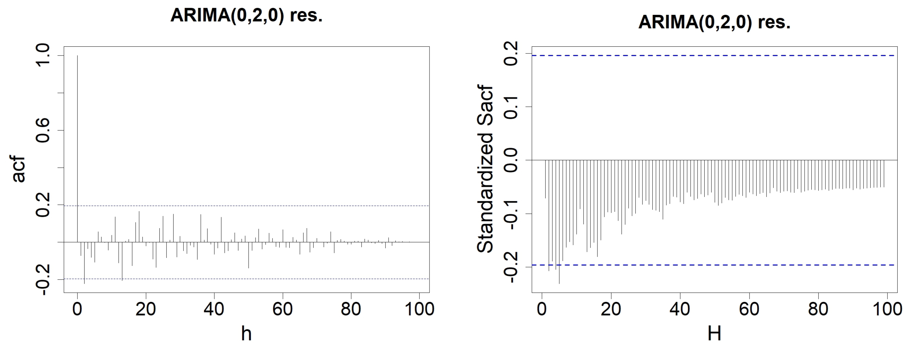
3.1. Sum of Sample Autocorrelation Functions (SACF)

Let us define the partial sum of the sample ACF values (Sacf) as follows:

$$S_{acf}\left(H\right)=\sum _{h=1}^H\widehat{\rho }\left(h\right),$$

(3)

and in the same way, we will call SACFand denote ${\displaystyle S_{ACF}\left(H\right)}$ as the sum of the associated sample ACF estimators. At any lag H, the associated SACF is a linear transformation of the random vector ${}^t(\widehat{\Xi }\left(1\right),\widehat{\Xi }\left(2\right),\cdots ,\widehat{\Xi }\left(H\right))$. It is well-known that any linear transformation of a multivariate Gaussian vector remains Gaussian. More precisely, we have the following proposition.

Proposition 1.

Let $\underline{Y}={}^t(Y_1,\cdots ,Y_r)$ be a multivariate Gaussian vector with distribution ${\mathcal{N}}_r(\underline{\mu },\Sigma )$, where $\underline{\mu }$ is a r vector and Σ is a $r\times r$ matrix, symmetric and definite-positive.

Then, for any matrix A in ${\mathbb{R}}^{p\times r}$, we have the following:

$$A^t(Y_1,\cdots ,Y_r)\sim {\mathcal{N}}_p(A\underline{\mu },A{\Sigma }^{t}A).$$

Note that because $\Sigma$ is symmetric and definite-positive, it implies that ${\displaystyle A{\Sigma }^{t}A}$ is also symmetric and definite-positive. Since the vector of the H first SACF ${}^t(S_{ACF}\left(1\right),S_{ACF}\left(2\right),\cdots ,$$S_{ACF}\left(H\right))$ is a linear transformation of the random vector ${}^t(\Xi \left(1\right),\Xi \left(2\right),\cdots ,\Xi \left(H\right))$ with a matrix $A_H$ being a squared and a unitary lower-triangular matrix, we obtain the following theorem:

Theorem 2.

Let ${\displaystyle Z_t={\mathcal{E}}_t}$ be white noise with ${\displaystyle \mathrm{I}\mathrm{E}\left({\mathcal{E}}_t^4\right)<\infty }$. Then,

$$\begin{array}{c}\hfill {\sqrt{n}}^t(S_{ACF}\left(1\right),S_{ACF}\left(2\right),\cdots ,S_{ACF}\left(H\right))\underset{n\to +\infty }{\overset{\mathcal{L}}{\to }}{\mathcal{N}}_H\left({}^t(0,\cdots ,0),{}^{t}W_H\right),\end{array}$$

where the diagonal terms of $W_H$ are $w_{i,i}=i$, and the non-diagonal terms are $w_{i,j}=min(i,j)$.

Let us denote by $\left({\mathcal{S}}_{\mathit{H}}(\underline{\mathit{\mu }},\mathbf{\Sigma })\right)$ as the property that ${\sqrt{n}}^t(S_{ACF}\left(1\right),S_{ACF}\left(2\right),\cdots ,S_{ACF}\left(H\right))$ is asymptotically multivariate Gaussian, with the expectation that the H vector $\underline{\mu }$ and covariance matrix $\Sigma$ are symmetric and definite-positive.

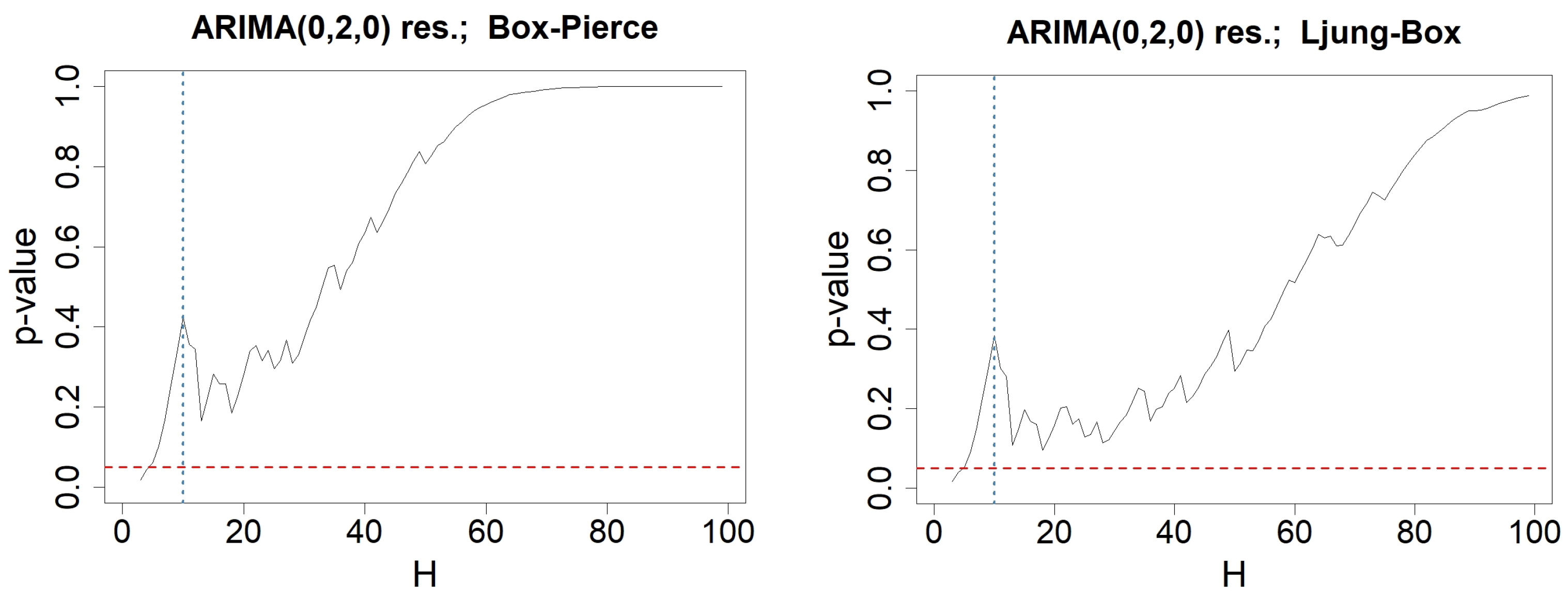
3.2. Diagnosis of White Noise (WN)

Based on Theorem 1, we determine that the random variables $\widehat{\Xi }\left(1\right),\widehat{\Xi }\left(2\right),\cdots ,\widehat{\Xi }\left(H\right)$ are asymptotically independent and identically distributed as Gaussian random variables with a zero mean and variance $1/n$. Consequently, for any fixed lag $h=1,\cdots ,H$, for large n, the sample autocorrelation function $\sqrt{n}\widehat{\rho }\left(h\right)$ is expected to be a realization of a standard Gaussian function that is to be valued in the interval of $[-1.96,1.96]$, with $95\%$ coverage. Thus, sample autocorrelation functions (ACF) are used to assess white noise.

But, even when the underlying process is white noise, several autocorrelations among $\widehat{\rho }\left(1\right),\cdots ,\widehat{\rho }\left(H\right)$ may lie out of the interval $[-1.96/\sqrt{n},1.96/\sqrt{n}]$. The asymptotic independence property for variables $\widehat{\Xi }\left(h\right)$ implies that when the sample size n is large the number of observed autocorrelation functions out of this interval must behave as having a binomial $\mathcal{B}(H,0.05)$ distribution. We can take into account the multiple testing paradigm by incorporating the binomial exact test and by incorporating a global testing procedure using Sidak’s correction [25].

Another way to summarize these multiple tests is to consider either Box–Pierce [12] or Ljung–Box statistics [19]:

$$\begin{array}{ccc}\hfill Q_{BP}& =& n\sum _{h=1}^n{\left(\widehat{\Xi }\left(h\right)\right)}^2,\hfill \end{array}$$

(4)

$$\begin{array}{ccc}\hfill Q_{LB}& =& n(n+2)\sum _{h=1}^n{\displaystyle \frac{1}{n-h}}{\left(\widehat{\Xi }\left(h\right)\right)}^2.\hfill \end{array}$$

(5)

The theoretical asymptotical distribution of these statistics is derived from the following property of multivariate Gaussian distributions.

Proposition 2.

Let ${\displaystyle \underline{Y}={}^t(Y_1,\cdots ,Y_H)}$ be a multivariate Gaussian function with a distribution of ${\displaystyle {\mathcal{N}}_H\left(\underline{\mu },\Sigma \right)}$, where ${\displaystyle \underline{\mu }}$ is an H vector of expectations and Σ is an $H\times H$ matrix that is symmetric and definite-positive. Then, for any real symmetric $H\times H$ matrix A with rank r:

1. 

If ${\displaystyle A\Sigma A=A}$, then ${\displaystyle {}^t\underline{Y}A\underline{Y}}$ is ${\chi }_s^2\left(\lambda \right)$ distributed, with $s=r$ and ${\displaystyle \lambda ={}^t\mu A\mu }$.

2. 

If ${\displaystyle {}^t\underline{Y}A\underline{Y}}$ is ${\chi }_s^2\left(\lambda \right)$ distributed, we have ${\displaystyle A\Sigma A=A}$, $s=r$ and ${\displaystyle \lambda ={}^t\mu A\mu }$.

Based on Theorem 1 and Proposition 2, the $Q_{BP}\left(H\right)$ statistic is supposed to behave as a ${\chi }_H^2$ distribution when the underlying process is a WN. Actually, Box–Pierce and Ljung–Box tests are widely used in practice when modeling time series using ARIMA($p,d,q$) models. Indeed, in the Box–Jenkins procedure, the estimated model is checked by applying Box–Pierce and Ljung–Box tests to the residuals of the model. In this case, the $Q_{BP}\left(H\right)$ statistic is supposed to behave as a ${\chi }_{H-p-q}^2$ distribution [41].

4. Theoretical Results

4.1. Contradiction with Theorems 1 and 2

If we apply the convergence in Theorem 2 with $H=n-1$, we obtain the following:

$$\sqrt{{\displaystyle \frac{n}{n-1}}}{S}_{ACF}(n-1)\sim \mathrm{A}\mathcal{N}\left(0,1\right)$$

(6)

where the symbol ∼ stands for “follows the distribution”, and $\mathrm{A}\mathcal{N}$ means “asymptotically Gaussian”. But, it is proved that [17] if $n\ge 2$,

$$S_{acf}(n-1)={\displaystyle \frac{1}{2}},$$

(7)

for any stationary time series, in particular for WN. Note that this result holds true for any time series with $n\ge 2$, even for the non-stationary ones. Since a Gaussian variable $\mathcal{N}(\mu ,{\sigma }^2)$ can be equal to the constant value $-{\displaystyle \frac{1}{2}}$ only if $\mu =-{\displaystyle \frac{1}{2}}$ and in the degenerate case ${\sigma }^2=0$, then Equations (6) and (7) appear to be contradictory. As a consequence, Theorem 2 does not hold for $H=n-1$, and neither does Theorem 1. Thus, $\left({\mathcal{A}}_{\mathit{n}-\mathbf{1}}(\underline{\mathbf{0}}, {\mathit{I}}_{\mathit{n}-\mathbf{1}})\right)$ does not hold.

However, let us suppose that $\left({\mathcal{A}}_{\mathit{n}-\mathbf{2}}(\underline{\mathbf{0}}, {\mathit{I}}_{\mathit{n}-\mathbf{2}})\right)$ is true. In particular, ${\sqrt{n}}^t(\widehat{\Xi }\left(1\right),\widehat{\Xi }\left(2\right),\cdots ,\widehat{\Xi }(n-2))$ is supposed to be asymptotically Gaussian multivariate. Since from Equation (7), we have:

$$\widehat{\Xi }(n-1)={\displaystyle \frac{1}{2}}-\sum _{h=1}^{n-2}\widehat{\Xi }\left(h\right),$$

(8)

then based on the definition of Gaussian vectors, ${\sqrt{n}}^t(\widehat{\Xi }\left(1\right),\widehat{\Xi }\left(2\right),\cdots ,\widehat{\Xi }(n-1))$ would also have an asymptotic multivariate distribution. More precisely,

$$\begin{array}{ccc}\hfill {\sqrt{n}}^t(\widehat{\Xi }\left(1\right),\widehat{\Xi }\left(2\right),\cdots ,\widehat{\Xi }(n-2),\widehat{\Xi }(n-1))& \sim & \mathrm{A}{\mathcal{N}}_{n-1}\left({}^t(0,\cdots ,0,-{\displaystyle \frac{1}{2}});\Sigma \right),\hfill \end{array}$$

with

$$\Sigma =\left(\begin{array}{ccccc}1& 0& \cdots & 0& -1\\ 0& 1& \cdots & 0& -1\\ ⋮& & ⋮& & ⋮\\ ⋮& & ⋮& & ⋮\\ 0& 0& \cdots & 1& -1\\ -1& -1& \cdots & -1& n-2\end{array}\right).$$

But this matrix is not definite positive, since $(1,\cdots ,1){\Sigma }^t(1,\cdots ,1)=0$.

Thus, $\left({\mathcal{A}}_{\mathit{n}-\mathbf{2}}(\underline{\mathbf{0}}, {\mathit{I}}_{\mathit{n}-\mathbf{2}})\right)$ is not true either.

Actually, Theorem 1, being an asymptotical result, needs H to remain lower than $n-1$ so that ${\displaystyle \frac{H}{n}}$ converges to 0. For instance, several authors recommend to take a sufficiently long time series ($n\ge 40$) and to consider only $H\le \sqrt{n}$ [42]. Therefore, $\left({\mathcal{A}}_{\mathit{H}}(\underline{\mathbf{0}}, {\mathit{I}}_{\mathit{H}})\right)$ should be true until $H\le \sqrt{n}$. And so Theorem 2 should also hold for $H\le \sqrt{n}$.

4.2. Asymptotic Normality

In this paper, we wonder if $\left({\mathcal{A}}_{\mathit{n}-\mathbf{1}}(\underline{\mathit{\mu }},\mathbf{\Sigma })\right)$ can be true, even for a non-zero vector $\underline{\mu }$ or for a covariance matrix $\Sigma$ that is not equal to the identity matrix. Let us denote ${\mu }_j$ as the coordinates of $\underline{\mu }$; ${\sigma }_j^2$ as the diagonal terms of $\Sigma$; and $c_{i,j}$ as the non-diagonal terms. Based on Equation (7) we would have the following:

$$\begin{array}{ccc}\hfill -{\displaystyle \frac{1}{2}}& =& \sum _{j=1}^{n-1}{\mu }_j\hfill \\ \hfill 0& =& \sum _{j=1}^{n-1}{\sigma }_j^2+2\sum _{i=1}^{n-2}\sum _{j=i+1}^{n-1}{c}_{i,j}.\hfill \end{array}$$

(9)

Since at least one variance ${\sigma }_j^2$ is positive (at least for $j\le \sqrt{n}$), then at least one covariance is not equal to zero. Consequently, $\Sigma$ is not diagonal. In other words, the sample ACFs are correlated, which is well-known from Hassani’s result (7). But Equation (9) also implies that $(1,\cdots ,1){\Sigma }^t(1,\cdots ,1)=0$, which means that the covariance matrix $\Sigma$ is not definite positive. Then, $\left({\mathcal{A}}_{\mathit{n}-\mathbf{1}}(\underline{\mathit{\mu }},\mathbf{\Sigma })\right)$ cannot be true, whatever $\underline{\mu }$ and $\Sigma$.

Furthermore, let us suppose that $\left({\mathcal{A}}_{\mathit{n}-\mathbf{2}}(\underline{\mathit{\mu }},\mathbf{\Sigma })\right)$ is true, where we denote ${\mu }_j$ tas he expectation coordinates, $c_{i,j}$ as the terms of the covariance matrix $\Sigma$, and ${\sigma }_j^2=c_{j,j}$ as the diagonal terms. In other words, ${\sqrt{n}}^t(\widehat{\Xi }\left(1\right),\widehat{\Xi }\left(2\right),\cdots ,\widehat{\Xi }(n-2))$ is supposed to be asymptotically Gaussian multivariate. Based on Equation (8) and based on the definition of Gaussian vectors, ${\sqrt{n}}^t(\widehat{\Xi }\left(1\right),\widehat{\Xi }\left(2\right),\cdots ,\widehat{\Xi }(n-1))$ would also have an asymptotic multivariate distribution. More precisely,

$$\begin{array}{ccc}\hfill {\sqrt{n}}^t(\widehat{\Xi }\left(1\right),\widehat{\Xi }\left(2\right),\cdots ,\widehat{\Xi }(n-2),\widehat{\Xi }(n-1))& \sim & \mathrm{A}{\mathcal{N}}_{n-1}\left({}^t(\underline{\mu },-{\displaystyle \frac{1}{2}}-\sum _{h=1}^{n-2}{\mu }_h);{\Sigma }^{\prime }\right),\hfill \end{array}$$

with ${\displaystyle {{\sigma }^2}_{n-1}^{\prime }=\sum _{j=1}^{n-2}{\sigma }_j^2+2\sum _{i=1}^{n-3}\sum _{j=i+1}^{n-2}{c}_{i,j}}$,

and for $i,j<n-1$, ${\displaystyle c_{n-1,j}^{\prime }=\sum _{h=1}^{n-2}{c}_{h,j}}$ and ${\displaystyle c_{i,n-1}^{\prime }=\sum _{h=1}^{n-2}{c}_{i,h}}$.

But matrix ${\Sigma }^{\prime }$ is not definite positive, since the following holds true:

$$\begin{array}{ccc}\hfill (1,\cdots ,1){\Sigma }^{\prime }{}^t(1,\cdots ,1)& =& 2{{\sigma }^2}_{n-1}^{\prime }-\sum _{j=1}^{n-2}{c}_{n-1,j}^{\prime }-\sum _{i=1}^{n-2}{c}_{i,n-1}^{\prime }\hfill \\ & =& 2\sum _{i,j=1}^{n-2}{c}_{i,j}-2\sum _{i,j=1}^{n-2}{c}_{i,j}\hfill \\ & =& 0.\hfill \end{array}$$

Thus, $\left({\mathcal{A}}_{\mathit{n}-\mathbf{2}}(\underline{\mathit{\mu }},\mathbf{\Sigma })\right)$ is not true either.

In this paper, we investigate the extent to which the property $\left({\mathcal{A}}_{\mathit{H}}(\underline{\mathit{\mu }},\mathbf{\Sigma })\right)$ is true, which has implications for the distribution of the associated SACF.

5. Simulation Results for WN

We simulate a white noise series to investigate the lag after which the distribution of the sample ACF and of the SACF no longer follow a normal distribution. Note that it is sufficient to consider standard white noise. Indeed, based on the definitions of theoretical and sample ACFs given in Equations (1) and (2), the underlying process ${\left(Z_t\right)}_t$ can be divided by its standard deviation without modifying the ACF values. When modeling, it is common to assume that the underlying white noise is Gaussian due to its favorable mathematical properties and simplicity. But in practice, the reality of the data may often present us with other distributions. Since we want to assess the persistence of the estimators’ normality, it makes sense to simulate white noise that lacks the typical properties of Gaussian white noise (symmetry, central peak). We have considered an example of a Gamma distribution, i.e., a centered exponential distribution. Actually, we run $N_S$ simulations of standard Gaussian WN and $N_S$ simulations of exponential WN of length $n=500$, with either $N_S=200$ or $N_S=5000$. For every simulation, we compute sample ACF and SACF values for $h=1,\cdots n-1$. We use the Shapiro–Wilk’s test [43] to assess for the normality. We also ran Lilliefors (composite Kolmogorov–Smirnov) normality test [44], which provided very similar results. Note that Shapiro and Lilliefors tests focus on the normality behavior of the sample, whatever the expectation and the variance of the underlying distribution. When the expectation $\mu$ and the variance ${\sigma }^2$ of the Gaussian distribution are explicit, we also run Kolmogorov–Smirnov’s test [45,46] to test the adequacy of the sample with the distribution $\mathcal{N}(\mu ,{\sigma }^2)$.

5.1. Check for the Normality of $\widehat{\Xi }\left(h\right)$ at a Fixed Lag h

At a given lag h, using the Kolmogorov–Smirnov test, we test for the adequacy of $\widehat{\Xi }\left(h\right)$ with the Gaussian distribution $\mathcal{N}\left(0,{\displaystyle \frac{1}{n}}\right)$, and we also merely test for its normality using the Shapiro–Wilk test. Figure 1 displays the p values provided by the Kolmogorov–Smirnov test when applied to either $N_S=200$ or $N_S=5000$ simulations of WN with length $n=500$. Figure 2 gives the p-values provided by the Shapiro–Wilk. Note that the same tests have also been conducting using WN with length $n=100$, and the results were very similar, as shown in the Supplementary Materials.

The results in the top line of Figure 1 show that $\widehat{\Xi }\left(h\right)$ behaves roughly like a Gaussian distribution $\mathcal{N}\left(0,{\displaystyle \frac{1}{n}}\right)$. This was expected based on Theorem 1, even for a lag h that was much greater than $\sqrt{n}$. But the graphics in the bottom line show that $\widehat{\Xi }\left(h\right)$ deviates from this specific normal distribution when we conduct the normality tests on more simulations. We recall that Theorem 1 provides an asymptotic result so that $\widehat{\Xi }\left(h\right)$ approximately follow the $\mathcal{N}\left(0,{\displaystyle \frac{1}{n}}\right)$ distribution. Its slight departure from this distribution is more easily detectable with a great number of simulations, and it is even more pronounced for exponential WN, meaning that the $\widehat{\Xi }\left(h\right)$ distribution may deviate from the $\mathcal{N}\left(0,{\displaystyle \frac{1}{n}}\right)$ theoretical distribution to a greater extent.

Nevertheless, if we focus on the Gaussian behavior of the ACF estimators $\widehat{\Xi }\left(h\right)$, Figure 2 shows that the normality behavior is fairly strong, especially for Gaussian WN, since Shapiro nearly never rejects the normality hypothesis, whatever the lag $h<n-2$, even with a great number of simulations $N_S=5000$. But for exponential WN, the normality property is quickly lost when the number of simulations increases.

Based on Figure 1 and Figure 2, we deduce that the lack of adequacy of $\widehat{\Xi }\left(h\right)$ from the distribution $\mathcal{N}\left(0,{\displaystyle \frac{1}{n}}\right)$ might come from its asymptotic property (explaining why it is more pronounced for exponential WN), but it appears that it also comes from a bad specification of the expectation and the variance (since the normality behavior is conserved, at least for Gaussian noises). Actually, $\widehat{\Xi }\left(h\right)$ may converge to a Gaussian distribution, but with either $\mu \ne 0$ or ${\sigma }^2\ne {\displaystyle \frac{1}{n}}$. Thus we obtain in particular that $\left({\mathcal{A}}_{\mathit{H}}(\underline{\mathbf{0}},{\mathit{I}}_{\mathit{H}})\right)$ is not true, but here, we have not obtained a contradiction with $\left({\mathcal{A}}_{\mathit{H}}(\underline{\mathit{\mu }},\mathbf{\Sigma })\right)$, which has to be explored.

5.2. Check for $\left({\mathcal{S}}_{\mathit{H}}(\underline{\mathit{\mu }},\mathbf{\Sigma })\right)$

At a given lag H, we test for the normality of the $N_S$ values of $S_{ACF}\left(H\right)$. Figure 3 displays the p-values provided by the Shapiro–Wilk test when applied to either $N_S=200$ or $N_S=5000$ simulations of WN with a length of $n=500$. Note that the same tests have also been conducted on WN with a length of $n=100$, and the results were very similar.

In Figure 3, we observe that the sum of sample ACFs departs from normality for almost all the lags H, except maybe for the first lags H, when the white noise is Gaussian and/or when the number of simulations remains low. Of course, the Kolmogorov–Smirnov test confirmed the departure of $S_{ACF}\left(H\right)$ from $\mathcal{N}\left(0,{\displaystyle \frac{H}{n}}\right)$ at any lag, whatever the nature of the WN (Gaussian or exponential) and even for a low number of simulations. The departure of $S_{ACF}\left(H\right)$ from $\mathcal{N}\left(0,{\displaystyle \frac{H}{n}}\right)$ can be explained by the previous finding that $\widehat{\Xi }\left(h\right)$ do not converge to a Gaussian distribution with $\mu =0$ and ${\sigma }^2={\displaystyle \frac{1}{n}}$.

But Figure 3 tells us that none of the variables $S_{ACF}\left(H\right)$ are Gaussian, so $\left({\mathcal{S}}_{\mathit{H}}(\underline{\mathit{\mu }},\mathbf{\Sigma })\right)$ can not be true, whatever $\mu$ and $\Sigma$. Thus, even the normality of the vector $(\widehat{\Xi }\left(1\right),\cdots ,\widehat{\Xi }\left(H\right))$ is called into question. Indeed, if $\left({\mathcal{A}}_{\mathit{H}}(\underline{\mathit{\mu }},\mathbf{\Sigma })\right)$ were true, then $\left({\mathcal{S}}_{\mathit{H}}(\underline{\mathit{\mu }},\mathbf{\Sigma })\right)$ would also be.

Consequently, based on Figure 2 and Figure 3, we conclude that at a fixed lag, h, $\widehat{\Xi }\left(h\right)$ is roughly Gaussian, with $\mu \simeq 0$ or ${\sigma }^2\simeq {\displaystyle \frac{1}{n}}$. But the vector $(\widehat{\Xi }\left(1\right),\cdots ,\widehat{\Xi }\left(H\right))$ is not a Gaussian vector. In other words, $\left({\mathcal{A}}_{\mathit{H}}(\underline{\mathit{\mu }},\mathbf{\Sigma })\right)$ is not satisfied. Hence, the reliability of the Box–Pierce and Ljung–Box tests is questioned, since they require $\left({\mathcal{A}}_{\mathit{H}}(\underline{\mathbf{0}},{\mathit{I}}_{\mathit{H}})\right)$.

5.3. Check for $\left({\mathcal{A}}_{\mathit{H}}(\underline{\mathit{\mu }},\mathbf{\Sigma })\right)$

The previous finding raises questions about the methods used in practice to model a time series. Indeed, a model has to be validated by checking that the associated residuals are WN by using Box–Pierce or Ljung–Box tests. We know that $\left({\mathcal{A}}_{\mathit{H}}(\underline{\mathbf{0}},{\mathit{I}}_{\mathit{H}})\right)$ does not hold. But, we wonder if it is a problem in practice. Then, we adopt another point of view that is more adequate with the practice, where we have to model a single time series from the properties of its first $\widehat{\rho }\left(h\right)$ values. For a given simulation, we test the normality of the set $\left(\widehat{\rho }\left(1\right),\cdots ,\widehat{\rho }\left(H\right)\right)$ when H varying from 1 to n − 1. This procedure appears to be adapted to check for the adequacy of $\left(\widehat{\rho }\left(1\right),\cdots ,\widehat{\rho }\left(H\right)\right)$ with a Gaussian vector, but it requires that the successive sample ACFs form a sample; in other words, that they are the realizations of the independent variables. Let us suppose that this hypothesis is satisfied. First, we use the Kolmogorov–Smirnov test to test for the adequacy of $\left(\widehat{\rho }\left(1\right),\cdots ,\widehat{\rho }\left(H\right)\right)$ with the Gaussian distribution $\mathcal{N}\left(0,{\displaystyle \frac{1}{n}}\right)$. Nexy, we use the Shapiro–Wilk test to test for the normality behavior. Figure 4 gives the percentage of inadequate testing conclusions when using the Kolmogorov–Smirnov test when applied to either $N_S=200$ or $N_S=5000$ simulations of WN with a length of $n=500$. Figure 5 gives the same percentages when using the Shapiro–Wilk test. Note that the same tests have also been conducted on WN with a length of $n=100$, and the results were very similar.

In Figure 4 and Figure 5, we observe that the percentage of p-values $<\alpha =5\%$ is very close to $5\%$, which seems to affirm that, at least for Gaussian WN, $\left(\widehat{\rho }\left(1\right),\cdots ,\widehat{\rho }\left(H\right)\right)$ can be considered as realizations of Gaussian variables until a lag H not too large based on the expectation and the covariance-matrix given in Theorem 1. These Figures seem to show that $\left({\mathcal{A}}_{\mathit{H}}(\underline{\mathit{\mu }},\mathbf{\Sigma })\right)$ and even $\left({\mathcal{A}}_{\mathit{H}}(\underline{\mathbf{0}},{\mathit{I}}_{\mathit{H}})\right)$ are true. This last point seems contradictory with Section 5.1 and Section 5.2. But, remember that the normality adequacy is sensitive to the number of observations used when applying the normality tests, and a slight departure from normality is more likely to be detected when this number is large. Here, the normality of the successive $\widehat{\rho }\left(1\right),\cdots ,\widehat{\rho }\left(H\right)$ values is assessed until a sample size of around $H={\displaystyle \frac{n}{2}}$ is obtained, which is low with respect to $N_S=5000$. Therefore, making a diagnosis from the first ACF might be acceptable. But, keep in mind that the tests displayed in Figure 4 and Figure 5 suppose that $\widehat{\rho }\left(1\right),\cdots ,\widehat{\rho }\left(H\right)$ are realizations of independent variables, which is not guaranteed. Indeed, Equation (7) proves that $\widehat{\rho }\left(1\right),\cdots ,\widehat{\rho }(n-1)$ cannot be independent.

6. Simulation Results for Residuals

6.1. Well-Specified Models

Since, in practice, white noise essentially appears as the residuals of an ARIMA($p,d,q$) model, we also ran simulations under several ARIMA($p,d,q$) models with either Gaussian or exponential underlying white noise. We simulated MA(2), AR(2), ARMA(1,1), ARIMA(0,2,2), and ARIMA(1,1,1) processes, as detailed in the Supplementary Materials. We estimated every simulated series with the convenient ARIMA($p,d,q$) model and computed its residuals. All the previous testing procedures introduced in Section 5 were applied to these residuals, and the obtained results are shown in a supplementary file on our web page. We obtained very similar results to those given in Section 5 for all the simulated models, ARIMA($p,d,q$).

More specifically, the deviation of the ACF from normality is highlighted mainly because of the flagrant non-normality of the SACF. It is also well-detected by Kolmogovov–Smirnov’s test with a larger number of simulations, meaning that the expected value and/or the expected variance of the ACF might not be well-specified. Departure from normality is more pronounced for the exponential WN, as detected using Shapiro’s normality test when the number of simulations increases. In addition to testing the normality of the $N_S$ ACF at a fixed lag h, we also adopt a point of view that is consistent with practical analyses, since we additionally test the fit of the successive ACFs with a Gaussian distribution. If the associated process is WN, the H successive ACFs should be identically normally distributed. Kolmogorov–Smirnov seems to perform very accurately, since the Type I error rate equals the nominal risk $\alpha$ until a rather large lag H. The Shapiro test also performs very well for residuals associated with ARIMA($p,d,q$) simulations with an underlying Gaussian WN, but it appears to be too liberal for underlying exponential WN. Furthermore, we show that the widely used Box–Pierce and Ljung–Box tests are not completely accurate. The Box–Pierce test appears to be too conservative, whereas the Ljung–Box test is too liberal.

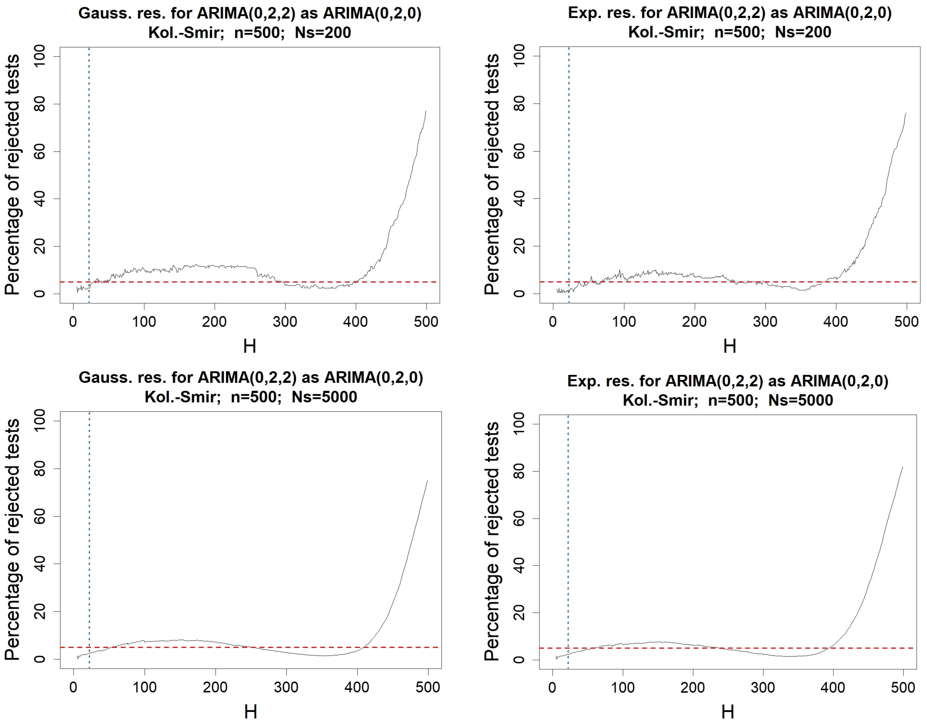
6.2. Misspecified Models

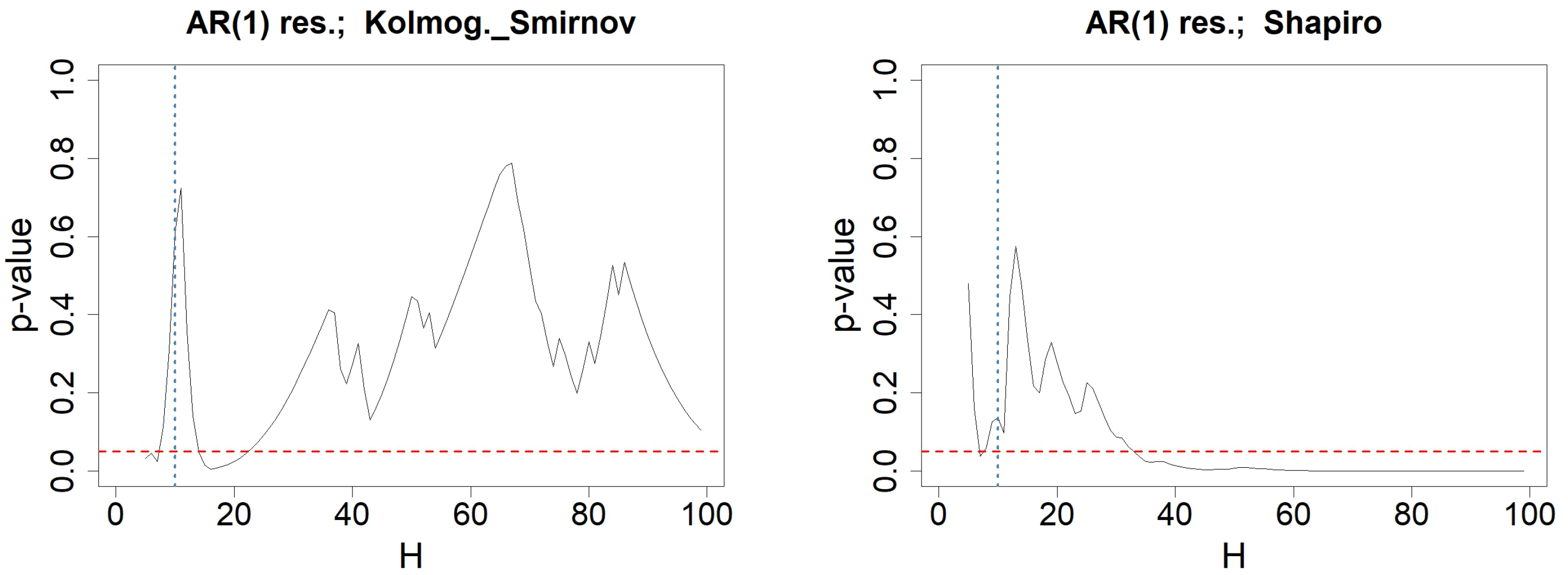
In the previous case, the orders of the underlying model were known, which is rarely the case, except when running simulations. In this section, we also explore the case where the estimated model is not the convenient one. We consider both the cases of too restrictive and too large model specifications. We run simulations under several ARIMA($p,d,q$) models with either Gaussian or an Exponential underlying white noise.

In the first case, we estimate every simulated series with an unsuitable ARIMA(p’,d’,q’) model, where $p^{\prime }<p$ and/or $d^{\prime }<d$ and/or $q^{\prime }<q$. We study the impact of using a too simple model ARMA(p’,d’,q’) when modeling the residuals using the previous testing procedures. We simulate MA(2), AR(2), ARIMA(0,2,2) and ARIMA(0,2,2) processes and estimate them by WN, WN, ARIMA(0,2,0), and AR(1) processes, respectively. In the main paper, we present the ARIMA(0,2,2) simulations estimated by an ARIMA(0,2,0). The other examples are detailed in the Supplementary Materials. In the second case, we proceed in the opposite way, estimating a more complicated model than the one used to generate the simulations. Actually, we simulate ARIMA(1,1,1) processes and estimate the simulated series with an ARIMA(2,1,2). This example is shown in the Supplementary Materials. All the previous testing procedures introduced in Section 5 were applied to the associated residuals, computed from the unsuitable ARIMA(p’,d’,q’) model.

In the first case of simulations (MA(2) simulations estimated by WN), the results are very similar to those observed in the main paper for simulations of an ARIMA(0,2,2), estimated by an ARIMA(0,2,0). Namely, only Shapiro’s test on successive ACFs and the portmanteau tests detected model mis-specifications. Note that these two cases only imply a mis-specification of the q parameter. The following case (AR(2) simulations estimated by WN) involving a mis-specification of the p parameter shows specific behaviors, as if the mis-specification were more pronounced. Indeed, Shapiro’s test on successive ACFs and the portmanteau tests still detect model mis-specifications, but additionally, Kolmogorov–Smirnov’s test applied either to the successive ACF or to the ACF at a fixed lag h detects a departure from normality. The third case (ARIMA(0,2,2) simulations estimated by an AR(1)) involves a mis-specification of all the parameters, p, d, and q. The testing procedures react as if the mis-specification were even more marked and more easily detectable. Thus, all the procedures systematically reject the null hypothesis of normality. Finally, the last simulations concern a mis-specification, but with a more general model than the one used to generate the simulations (ARIMA(1,1,1) simulations estimated by an ARIMA(2,1,2)). In this case, the testing procedures provide results that are very similar to WN or the residuals of well-specified models.

Here, we focus on the ARIMA(0,2,2) process, as this is the model that will be used to model the example in the next section. We simulate an ARIMA(0,2,2) with the following equation:

$${\Delta }^2\left(Z_t\right)={\mathcal{E}}_t-{\displaystyle \frac{3}{4}}{\mathcal{E}}_{t-1}+{\displaystyle \frac{1}{8}}{\mathcal{E}}_{t-2},$$

where ${\left({\mathcal{E}}_t\right)}_t$ is either Gaussian or exponential WN with a length $n=500$. But, instead of considering the convenient ARIMA(0,2,2) model, we estimate the simulated process using an ARIMA(0,2,0) model. We suppose that the order difference d is well-estimated from unit-root tests [47,48,49] or by using a more complex protocol [25]. In the Supplementary Materials, we model ARIMA(0,2,0) simulations using a more restrictive AR(1) model. In this more restrictive case, we determine that all the testing procedures computed on the successive ACFs (Kolmogorov–Smirnov, Shapiro, Box–Pierce and Ljung–Box tests) drastically reject the null hypothesis, warning that the model is mis-specified.

6.3. Check for the Normality of $\widehat{\Xi }\left(h\right)$ at a Fixed Lag h

At a given lag h, using the Kolmogorov–Smirnov test, we test for the adequacy of $\widehat{\Xi }\left(h\right)$ with the Gaussian distribution $\mathcal{N}\left(0,{\displaystyle \frac{1}{n}}\right)$, and we also merely test for its normality using the Shapiro–Wilk test. Figure 6 displays the p-values provided by the Kolmogorov–Smirnov test when applied to either $N_S=200$ or $N_S=5000$ simulations of WN with length $n=500$. Figure 7 gives the p-values provided by the Shapiro–Wilk test.

Here, we observe the same behavior as that of the simulated WN. Indeed, in Figure 7, we see that Shapiro’s test does not reject the normality of the ACFs at a fixed lag h, but Kolmogorov–Smirnov’s test detects a lack of fit to the expected normal distribution $\mathcal{N}\left(0,{\displaystyle \frac{1}{n}}\right)$ as the number of simulations increases; see Figure 6. This means that the ACFs follow a distribution that is close to a normal distribution, but with either an expectation different from 0 and/or variance that is different from ${\displaystyle \frac{1}{n}}$.

6.4. Check for the Normality of $SACF\left(H\right)$ at a Fixed Lag H

At a given lag H, we test for the normality of the $N_S$ values of $S_{ACF}\left(H\right)$. Figure 8 displays the p-values provided by the Shapiro–Wilk test when applied to either $N_S=200$ or $N_S=5000$ simulations of WN with a length of $n=500$.

The SACF associated with WN simulations or with residuals from well-specified models did not behave at all like normal distributions, contrary to what might be expected, even with a small number of simulations. Here, in Figure 8, the departure from normality is less obvious, especially when the underlying WN is Gaussian.

6.5. Check for $\left({\mathcal{A}}_{\mathit{H}}(\underline{\mathit{\mu }},\mathbf{\Sigma })\right)$

For a given simulation, we test the normality of the set $\left(\widehat{\rho }\left(1\right),\cdots ,\widehat{\rho }\left(H\right)\right)$, with H varying from 1 to n − 1. This procedure appears to be adapted to check for the adequacy of $\left(\widehat{\rho }\left(1\right),\cdots ,\widehat{\rho }\left(H\right)\right)$ with a Gaussian vector, but it requires that the successive sample ACFs form a sample; in other words, it requires that they are the realizations of independent variables. Let us suppose that this hypothesis is satisfied. First, we use the Kolmogorov–Smirnov test to test for the adequacy of $\left(\widehat{\rho }\left(1\right),\cdots ,\widehat{\rho }\left(H\right)\right)$ with the Gaussian distribution $\mathcal{N}\left(0,{\displaystyle \frac{1}{n}}\right)$. Next, we use the Shapiro–Wilk test to test for the normality behavior. Figure 9 gives the percentage of inadequate testing conclusions when using the Kolmogorov–Smirnov test applied to either $N_S=200$ or $N_S=5000$ simulations of ARIMA(0,2,2) processes estimated by an ARIMA(0,2,0). Figure 10 gives the same percentages based on the Shapiro–Wilk test.

In Figure 9, we observe that the percentage of p-values $<\alpha =5\%$ for the Kolmogorov–Smirnov test is very close to $5\%$, which seems to affirm that $\left(\widehat{\rho }\left(1\right),\cdots ,\widehat{\rho }\left(H\right)\right)$ can be considered as realizations of Gaussian variables $\mathcal{N}\left(0,{\displaystyle \frac{1}{n}}\right)$, until a rather large lag H value, as if the residuals were WN. But, as seen in Figure 10, Shapiro’s test largely rejects the normality condition for the successive ACFs. Shapiro’s test on successive ACFs is the only normality test that is sensitive to the fact that the model is mis-specified, alerting us to the fact that the residuals probably do not form white noise. Indeed, Figure A2 in Appendix B shows that portmanteau tests do not validate the proposed model.

7. Illustration Using an Economic Data Set

We consider money stock evolution in USA, given in billions of USD and annual averages from 1889 to 1988 [2]. See Figure 11 (Left), for its evolution. This money stock series has unit roots and should be modeled by an ARIMA(0,2,2) model [25]. We study the associated residuals, displayed in Figure 11 (Right). If the model is well-calibrated, the residuals should behave as WN. Then, we plot the successive ACFs of the residuals in Figure 12 (left), and we test their normality (Figure 13 (right)) and their adequacy to a $\mathcal{N}\left(0,{\displaystyle \frac{1}{n}}\right)$ distribution (Figure 13 (Left)). We observe that the set of the successive ACFs $\left(\widehat{\rho }\left(1\right),\cdots \widehat{\rho }\left(H\right)\right)$ behaves as a $\mathcal{N}\left(0,{\displaystyle \frac{1}{n}}\right)$ distribution, except when H becomes too close to $n-1$, as expected based on Section 4.2. Let us note that the residuals are not Gaussian-distributed, since the Shapiro–Wilk test provides a p-value equal to $0.008$. Hence, we are in the situation where the departure from normality is more accentuated for the ACF at a given lag (see Figure 2 (bottom right)), and for the set of the successive ACFs $\left(\widehat{\rho }\left(1\right),\cdots ,\widehat{\rho }\left(H\right)\right)$ (see Figure 5 (right)). To further explore the possible departure of ACF from normality, we plot in Figure 12 (right) the successive standardized SACF ${\displaystyle \frac{S_{ACF}\left(H\right)}{\sqrt{H}}}$. If the conditions are close enough to $\left({\mathcal{A}}_{\mathit{H}}(\underline{\mathbf{0}},{\mathit{I}}_{\mathit{H}})\right)$, then every standardized SACF should behave as a $\mathcal{N}\left(0,{\displaystyle \frac{1}{n}}\right)$ distribution. In other words, most standardized SACF should lie inside the interval of $[-1.96/\sqrt{n},1.96/\sqrt{n}]$, plotted with blue dashed lines. Figure 12 (right) shows that the SACFbehave rather well, implying that the ACFs themselves have sufficiently satisfactory normality properties for the Box–Pierce and the Ljung–Box tests to be reliable. Finally, in Figure 14, both portmanteau tests are computed successively for all lags $H=1,\cdots ,n-1$ to assess for the validity of the constructed model, which can be used for prediction.

Note that we ran the same testing procedures when modeling money stock series using an ARIMA(0,2,0); see Figure A3, Figure A4 and Figure A5 in Appendix C. The ARIMA(0,2,0) model results in an interesting alternative model. But, by using cross-validation (training on 95%, testing on 5%) and by computing the RMSE and MAPE criteria between the predictions and the test set, we determine that the ARIMA(0,2,2) model is better (see

Table A1. Models comparison for money stock series.

Model	RMSE	MAPE
ARIMA(0,2,2)	0.095	0.122
ARIMA(0,2,0)	0.141	1.649
AR(1)	0.255	3.156

). Now, let us estimate a false model for these data with parameters that are too restrictive, such as an AR(1) model. We apply the same statistical procedures to the produced residuals. In Figure 15, we observe that several ACFs and numerous standardized SACFare well outside the reference interval $[-1.96/\sqrt{n},1.96/\sqrt{n}]$. Next, contrary to the ARIMA(0,2,2) model, Shapiro’s test on the successive ACFs rejects the hypothesis of normality for numerous lags h (Figure 16). Finally, both portmanteau tests detect the model mis-specification (Figure 17). As a conclusion, we find that almost all the procedures (except for the Kolmogorov–Smirnov test) exhibit a very different behavior from the first case when the model was well-specified.

8. Discussion

According to the theoretical results, the ACF and SACF of innovations in an ARIMA ($p,d,q$) process are normally distributed. In this study, we simulate WN, either Gaussian or exponential, and we also simulate various ARIMA($p,d,q$) process. We estimate every simulated series using an ARIMA(p’,d’,q’) model and compute its residuals. We test the normality of both the ACFs and the SACFs of these residuals. When the estimated ARIMA(p’,d’,q’) model matches the model used for the simulation, all the previous testing procedures introduced in Section 5 are similar to the ones observed for WN simulations.

Thus, we observed that $\widehat{\Xi }\left(h\right)$ behaves roughly like a Gaussian distribution $\mathcal{N}\left(0,{\displaystyle \frac{1}{n}}\right)$, as it was expected based on Theorem 1, even for a lag h much greater than $\sqrt{n}$. Its slight departure from this distribution is more pronounced for exponential WN. We can deduce that the lack of adequacy of $\widehat{\Xi }\left(h\right)$ from the distribution $\mathcal{N}\left(0,{\displaystyle \frac{1}{n}}\right)$ might come from its asymptotic property (explaining why it is more pronounced for exponential WN), but it also comes from a bad specification of the expectation and the variance (since the normality behavior is conserved, at least for Gaussian noise). Actually, $\widehat{\Xi }\left(h\right)$ may converge to a Gaussian distribution, but with either $\mu \ne 0$ or ${\sigma }^2\ne {\displaystyle \frac{1}{n}}$.

Moreover, we found evidence that the sum of sample ACFs $S_{ACF}\left(H\right)$ departs from normality for almost all the lags H, except maybe for the first lags H when the white noise is Gaussian. This implies that the vector $\left(\widehat{\rho }\left(1\right),\cdots \widehat{\rho }\left(H\right)\right)$ is not likely to be a Gaussian vector. Therefore, Theorem 1 should be applied with caution.

Nevertheless, in practice, at least for Gaussian WN, $\widehat{\rho }\left(1\right),\cdots ,\widehat{\rho }\left(H\right)$ roughly behave as realizations of Gaussian variables until a lag H that is not too large, with the expectation and the covariance matrix close to the ones stated in Theorem 1. Consequently, one can make a diagnosis that is rather reliable based on the rule that, at a fixed lag h that is not too large, ACF $\widehat{\rho }\left(h\right)$ should lie inside the interval $[-1.96/\sqrt{n},1.96/\sqrt{n}]$. But, the asymptotic covariance matrix might not be diagonal, meaning that ACF independence might not be satisfied. Then, the current and widely used techniques, such as Box–Pierce and Ljung–Box tests or a binomial procedure, do not reliably take multiple testings into account, since they suppose their independence.

We explored the reliability of Box–Pierce and Ljung–Box tests using our simulations by applying these tests to every simulation at lags of $H=1$ to $n-1$. We computed the percentage of unexpected p-values ($<\alpha =5\%$) among the $N_S$ simulations. We observed that the portmanteau tests are not completely accurate. Indeed, the Box–Pierce test appears to be too conservative, whereas the Ljung–Box test is too liberal. The low reliability of the Ljung–Box test has already been identified in [50], and several authors have given several empirical rules to improve its reliability, notably by limiting the lag H to which it could be applied. Among them, we have different suggestions, such as $H\le {\displaystyle \frac{n}{4}}$ [13], $H\le min\left(20,{\displaystyle \frac{n}{4}}\right)$ [51], $H\le ln\left(n\right)$ [5], and more explicit lags obtained using simulation procedures [52].

But, a better estimation of the expectation vector and of the covariance matrix in Theorem 1 could permit us to improve their performance by using Proposition 2. However, we suspect that the asymptotic behavior of the ACF vector $\left(\widehat{\rho }\left(1\right),\cdots ,\widehat{\rho }\left(H\right)\right)$ might not even be multivariate Gaussian. In other words, $\left({\mathcal{A}}_{\mathit{H}}(\underline{\mathit{\mu }},\mathbf{\Sigma })\right)$ might not be true, whatever $\underline{\mu }$ and $\Sigma$. In this case, Proposition 2 could not be applied, and we would have to take a different point of view in order to develop a test to check the adequacy of a time series with white noise.

In practice, the main risk is the lack of reliability of portmanteau tests when validating an ARIMA($p,d,q$) model. But, among all the testing procedures, several perform accurately when we estimate the simulated series with the convenient ARIMA($p,d,q$) model and compute its residuals. Thus, Kolmogorov–Smirnov’s test applied to the successive ACFs performs very accurately, since the Type I error rate is equal to the nominal risk $\alpha$, whatever the nature of the underlying WN. This is also the case for Shapiro’s test applied to the successive ACFs when the underlying WN is Gaussian.

We also explore the case where the estimated model is not the convenient one. In the case of model specifications that are too liberal, the results are similar to the well-specified model. But, in the case of model specifications that are too restrictive, the testing procedures produce very different results. When only q is mis-specified, only Shapiro’s test on successive ACFs and the portmanteau tests detect model mis-specification. When only p is mis-specified, Shapiro’s test on successive ACFs and the portmanteau tests still detect model mis-specification, but additionally, Kolmogorov–Smirnov’s test applied either to the successive ACF or to the ACF at a fixed lag h detects a departure from normality. And finally, when parameter d is involved, the testing procedures react as if the mis-specification were even more marked; therefore, it is more easily detectable. Indeed, all the procedures systematically reject the null hypothesis of normality.

Thus, in the case of model specifications that are too restrictive, the estimated residuals do not satisfy white noise conditions, which are detected by portmanteau tests. Note that Shapiro’s test on the successive ACFs $\left(\widehat{\rho }\left(1\right),\cdots ,\widehat{\rho }\left(H\right)\right)$ is the only other procedure that clearly differentiates the diagnosis between the residuals of a well-specified or of a mis-specified model. The Kolmogorov–Smirnov test is less sensitive, in particular when only the parameter q is mis-specified. Thus the non-normality of the successive ACFs is a good signal of the inaccurate model specifications.

Consequently, when portmanteau tests validate an ARIMA model, we suggest to check for portmanteau test relevance by checking the correct behavior of the successive ACFs by testing the adequacy of $\widehat{\rho }\left(1\right),\cdots ,\widehat{\rho }\left(H\right)$ with a $\mathcal{N}\left(0,{\displaystyle \frac{1}{n}}\right)$ distribution, or simply, its normality. If the ACFs show Gaussian behaviors, the validation of the model provided by the portmanteau tests might be reliable. In the opposite case, the portmanteau tests might not be reliable. If the model is mis-specified with a model that is too restrictive, it might be detected by portmanteau tests and by the departure of the successive ACFs from normality.

References

1. Elsaraiti, M.; Musbah, H.; Merabet, A.; Little, T. Time Series Analysis of Electricity Consumption Forecasting Using ARIMA Model. IEEE Green Technol. Conf. 2021, 259–262. [Google Scholar] [CrossRef]
2. Nelson, C.R.; Plosser, C.I. Trends and Random Walks in Macroeconomic Time Series: Some Evidence and Implications. J. Monet. Econ. 1982, 10, 139–162. [Google Scholar] [CrossRef]
3. Ogunlana, S.O.; Oyebisi, T.O. Modelling and Forecasting Nigerian Electricity Demand Using Univariate Box-Jenkins Approach. J. Energy Technol. Policy 2013, 3, 84–91. [Google Scholar]
4. Pena, D.; Rodriguez, J. Forecasting Traffic Flow by Using Time Series Models. Transp. Rev. 2001, 21, 293–317. [Google Scholar]
5. Tsay, R. Analysis of Financial Time Series, 3rd ed.; John Wiley & Sons: New York, NY, USA, 2010. [Google Scholar]
6. Teyssière, G.; Kirman, A. Microeconomic models for long memory in the volatility of financial time series. Physics A 2002, 370, 26–31. [Google Scholar]
7. Arunachalam, V.; Jaafar, A. Forecasting Dengue Incidence in Penang, Malaysia: A Comparison of ARIMA and GARCH Models. Am. J. Trop. Med. Hyg. 2011, 85, 827–833. [Google Scholar]
8. Glass, G.V.; Willson, V.L.; Gottman, J.M. Design and Analysis of Time-Series Experiments. Annu. Rev. Psychol. 1975, 26, 609–653. [Google Scholar]
9. Luis, C.O.; Francisco, G.S.; Jose, M.S. Forecasting of Emergency Department Admissions. Healthc. Manag. Sci. 2012, 15, 215–224. [Google Scholar]
10. Campbell, J.Y.; Perron, P. An Empirical Investigation of the Relations between Climate Change and Agricultural Yield: A Time Series Analysis of Maize Yield in Nigeria. J. Agric. Environ. Sci. 2004, 5, 217–230. [Google Scholar]
11. Zheng, X.; Basher, R.E. Structural Time Series Models and Trend Detection in Global and Regional Temperature Series. J. Clim. 1999, 12, 2347–2358. [Google Scholar] [CrossRef]
12. Box, G.; Pierce, D. Distribution of Residual Autocorrelations in Autoregressive-Integrated Moving Average Time Series Models. J. Am. Statist. Assoc. 1970, 65, 1509–1526. [Google Scholar] [CrossRef]
13. Brockwell, P.; Davis, R. Time Series: Theory and Methods, 2nd ed.; Springer: New York, NY. USA, 1991. [Google Scholar]
14. Brockwell, P.J.; Davis, R.A. Introduction to Time Series and Forecasting; STS; Springer: Cham, Switzerland, 2016. [Google Scholar]
15. Chatfield, C. The Analysis of Time Series: An Introduction; CRC Press: Boca Raton, FL, USA, 2003. [Google Scholar]
16. Hamilton, J.D. Time Series Analysis. Econom. Rev. 1994, 13, 147–192. [Google Scholar]
17. Hassani, H. Sum of the sample of autocorrelation function. Random Oper. Stoch. Eqs. 2009, 17, 125–130. [Google Scholar] [CrossRef]
18. Hyndman, R.J.; Athanasopoulos, G. Forecasting: Principles and Practice. Int. J. Forecast. 2018, 34, 587–590. [Google Scholar]
19. Ljung, G.; Box, G. On a Measure of a Lack of Fit in Time Series Models. Biometrika 1978, 65, 297–303. [Google Scholar] [CrossRef]
20. Montgomery, D.C.; Jennings, C.L.; Kulahci, M. Introduction to Time Series Analysis and Forecasting; John Wiley & Sons: Hoboken, NJ, USA, 2008. [Google Scholar]
21. Priestley, M.B. Spectral Analysis and Time Series. J. Time Ser. Anal. 1981, 2, 85–106. [Google Scholar] [CrossRef]
22. Shumway, R.H.; Stoffer, D.S. Time Series Analysis and Its Applications: With R Examples; Springer: Berlin/Heidelberg, Germany, 2006. [Google Scholar]
23. Wei, W.W.S. Time Series Analysis Univariate and Multivariate Methods, 2nd ed.; Addison Wesley: New York, NY, USA, 2006. [Google Scholar]
24. Bisaglia, L.; Gerolimetto, M. Testing for Time Series Linearity Using the Autocorrelation Function. Stat. Methods Appl. 2009, 18, 23–50. [Google Scholar]
25. Boutahar, M.; Royer-Carenzi, M. Identifying trends nature in time series using autocorrelation functions and stationarity tests. Int. J. Econ. Econom. 2024, 14, 1–22. [Google Scholar] [CrossRef]
26. Kendall, M.G. Time-Series; Oxford University Press: Oxford, UK, 1976. [Google Scholar]
27. McLeod, A.I.; Zhang, Y. Partial Autocorrelation Parameterization for Seasonal ARIMA Models. Int. J. Forecast. 2006, 22, 661–673. [Google Scholar]
28. Granger, C.W.J.; Joyeux, R. An Introduction to Long-Memory Time Series Models and Fractional Differencing. J. Time Ser. Anal. 1980, 1, 15–29. [Google Scholar] [CrossRef]
29. Hassani, H.; Yarmohammadi, M.; Mashald, L. Uncovering hidden insights with long-memory-proscess detection: An in-depth overview. Risks 2023, 11, 113. [Google Scholar] [CrossRef]
30. Hosking, J. Asymptotic distribution of the sample mean, autocovariances, autocorrelations of long-memory time series. J. Econom. 1996, 73, 261–284. [Google Scholar] [CrossRef]
31. Dimitriadis, P.; Koutsoyiannis, D. Climacogram versus Autocovariance and Power Spectrum in Stochastic Modelling for Markovian and Hurst-Kolmogorov Processes. Stoch. Environ. Res. Risk Assess. 2015, 15, 1649–1669. [Google Scholar] [CrossRef]
32. Liu, S.; Xie, Y.; Fang, H.; Du, H.; Xu, P. Trend Test for Hydrological and Climatic Time Series Considering the Interaction of Trend and Autocorrelations. Water 2022, 14, 3006. [Google Scholar] [CrossRef]
33. Phojanamongkolkij, N.; Kato, S.; Wielicki, B.A.; Taylor, P.C.; Mlynczak, M.G. A Comparison of Climate Signal Trend Detection Uncertainty Analysis Methods. J. Clim. 2014, 27, 3363–3376. [Google Scholar] [CrossRef]
34. Xie, Y.; Liu, S.; Fang, H.; Wang, J. Global Autocorrelation Test Based on the Monte Carlo Method and Impacts of Eliminating Nonstationary Components on the Global Autocorrelation Test. Stoch. Environ. Res. Risk Assess. 2020, 34, 1645–1658. [Google Scholar] [CrossRef]
35. Belmahdi, B.; Louzazni, M.; El Bouardi, A. One month-ahead forecasting of mean daily global solar radiation using time series models. Optik 2020, 219, 165207. [Google Scholar] [CrossRef]
36. Gostischa, J.; Massolo, A.; Constantine, R. Multi-species feeding association dynamics driven by a large generalist predator. Front. Mar. Sci. 2021, 8, 739894. [Google Scholar] [CrossRef]
37. Yang, Y.; Qin, S.; Liao, S. Ultra-chaos of a mobile robot: A higher disorder than normal-chaos. Chaos. Solitons Fractals 2023, 167, 113037. [Google Scholar] [CrossRef]
38. Bai, M.; Zhou, Z.; Chen, Y.; Liu, J.; Yu, D. Accurate four-hour-ahead probabilistic forecast of photovoltaic power generation based on multiple meteorological variables-aided intelligent optimization of numeric weather prediction data. Earth Sci. Inform. 2023, 16, 2741–2766. [Google Scholar] [CrossRef]
39. Orlando, G.; Bufalo, M. Empirical evidences on the interconnectedness between sampling and asset returns’s distributions. Risks 2021, 9, 88. [Google Scholar] [CrossRef]
40. Wang, X.; Yang, J.; Yang, F.; Wang, Y.; Liu, F. Multilevel residual prophet network time series model for prediction of irregularities on high-speed railway track. J. Transp. Eng. Part Syst. 2023, 149, 04023012. [Google Scholar] [CrossRef]
41. Li, W. Diagnostic Checks in Time Series; Monographs on Statistices and Applied Probability; Chapman & Hall: New York, NY, USA, 2004; Volume 102. [Google Scholar]
42. Box, G.; Jenkins, G.; Reinsel, G.C. Time Series Analysis: Forecasting and Control, 3rd ed.; Prentice Hall: Englewood Clifs, NJ, USA, 1994. [Google Scholar]
43. Shapiro, S.; Wilk, M. An Analysis of Variance Test for Normality (Complete Samples). Biometrika 1965, 52, 591–611. [Google Scholar] [CrossRef]
44. Dallal, G.; Wilkinson, L. An analytic approximation to the distribution of lilliefors’ test for normality. Am. Stat. 1986, 40, 294–296. [Google Scholar] [CrossRef]
45. Kolmogorov, A. Sulla determinazione empirica di una legge di distribuzione. G. Ist. Ital. Attuari 1933, 4, 83–91. [Google Scholar]
46. Smirnov, N. Table for estimating the goodness of fit of empirical distributions. Ann. Math. Statist. 1948, 19, 279–281. [Google Scholar] [CrossRef]
47. Dickey, D.A.; Fuller, W.A. Distribution of the Estimators for Autoregressive Time Series with a Unit Root. J. Am. Stat. Assoc. 1979, 74, 427–431. [Google Scholar]
48. Dickey, D.A.; Fuller, W.A. Likelihood Ratio Statistics for Autoregressive Time Series with a Unit Root. Econometrica 1981, 49, 1057–1072. [Google Scholar] [CrossRef]
49. Phillips, P.C.B.; Perron, P. Testing for a unit root in time series regression. Biometrika 1988, 75, 335–346. [Google Scholar] [CrossRef]
50. Hassani, H.; Yeganegi, M. Sum of squared ACF and the Ljung-Box statistic. Physics A 2019, 520, 80–86. [Google Scholar] [CrossRef]
51. Anderson, O. The box-jenkins approach to time series analysis. RAIRO 1977, 11, 3–29. [Google Scholar] [CrossRef]
52. Hassani, H.; Yeganegi, M. Selecting optimal lag order in Ljung-Box test. Physics A 2020, 541, 123700. [Google Scholar] [CrossRef]
Figure 1. p-values when testing for the adequacy of the N S values of ρ ^ ( h ) with N 0 , 1 n , for any fixed lag h varying from 1 to n 1 . The involved normality test is Kolmogorov–Smirnov’s. The left column concerns Gaussian WN, whereas the right one deals with the exponential WN process. The length of the simulated WN process is n = 500 . In the upper figures, the number of simulated WN processes is N S = 200 , whereas it is N S = 5000 in the bottom. The red-dotted horizontal line represents 5 % , while the blue-dotted vertical line represents h = n .
Information 15 00449 g001
Figure 2. p-values when testing for the normality of the N S values of ρ ^ ( h ) for any fixed lag h varying from 1 to n 1 . The involved normality test is Shapiro–Wilk’s. The left column concerns Gaussian WN, whereas the right one deals with the exponential WN process. The length of the simulated WN process is n = 500 . In the upper figures, the number of simulated WN processes is N S = 200 , whereas it is N S = 5000 in the bottom. The red-dotted horizontal line represents 5 % , while the blue-dotted vertical line represents h = n .
Information 15 00449 g002
Figure 3. p-values when testing for the normality of the N S values of S a c f ( H ) for any fixed lag H varying from 1 to n 1 . The involved normality test is Shapiro–Wilk’s. The left column concerns Gaussian WN, whereas the right one deals with the exponential WN process. The length of the simulated WN process is n = 500 . In the upper figures, the number of simulated WN processes is N S = 200 , whereas it is N S = 5000 in the bottom. The red-dotted horizontal line represents 5 % , while the blue-dotted vertical line represents H = n .
Information 15 00449 g003
Figure 4. Percentage of unexpected p-values ( < α = 5 % ) when testing for the normality of ρ ^ ( 1 ) , , ρ ^ ( H ) with N 0 , 1 n when H varies from 1 to n 1 . The involved normality test is Kolmogorov–Smirnov’s. The left column concerns Gaussian WN, whereas the right one deals with the exponential WN process. In the upper figures, the number of simulated WN processes is N S = 200 , whereas it is N S = 5000 in the bottom. The red-dotted horizontal line represents 5 % , while the blue-dotted vertical line represents H = n .
Information 15 00449 g004
Figure 5. Percentage of unexpected p-values ( < α = 5 % ) among the N S simulations when testing for the normality of ρ ^ ( 1 ) , , ρ ^ ( H ) with H varying from 1 to n 1 . The involved normality test is Shapiro–Wilk’s. The left column concerns Gaussian WN, whereas the right one deals with the exponential WN process. The length of the simulated WN process is n = 500 . In the upper figures, the number of simulated WN processes is N S = 200 , whereas it is N S = 5000 in the bottom. The red-dotted horizontal line represents 5 % , while the blue-dotted vertical line represents H = n .
Information 15 00449 g005aInformation 15 00449 g005b
Figure 6. p-values when testing for the adequacy of the N S values of ρ ^ ( h ) with N 0 , 1 n for any fixed lag h varying from 1 to n 1 . The involved normality test is Kolmogorov–Smirnov’s. The left column concerns Gaussian underlying W,N whereas the right one deals with the exponential underlying WN process. The length of the simulated WN process is n = 500 . In the upper figures, the number of simulated WN processes is N S = 200 , whereas it is N S = 5000 in the bottom. The red-dotted horizontal line represents 5 % , while the blue-dotted vertical line represents h = n .
Information 15 00449 g006
Figure 7. p-values when testing for the normality of the N S values of ρ ^ ( h ) for any fixed lag h varying from 1 to n 1 . The involved normality test is Shapiro–Wilk’s. The left column concerns Gaussian underlying WN, whereas the right one deals with the exponential underlying WN process. The length of the simulated WN process is n = 500 . In the upper figures, the number of simulated WN processes is N S = 200 , whereas it is N S = 5000 in the bottom. The red-dotted horizontal line represents 5 % , while the blue-dotted vertical line represents h = n .
Information 15 00449 g007
Figure 8. p-values when testing for the normality of the N S values of S a c f ( H ) for any fixed lag H varying from 1 to n 1 . The involved normality test is Shapiro–Wilk’s. The left column concerns Gaussian underlying WN, whereas the right one deals with exponential WN. The length of the simulated WN process is n = 500 . In the upper figures, the number of simulated WN processes is N S = 200 , whereas it is N S = 5000 in the bottom. The red-dotted horizontal line represents 5 % , while the blue-dotted vertical line represents H = n .
Information 15 00449 g008
Figure 9. Percentage of unexpected p-values ( < α = 5 % ) when testing for the normality of ρ ^ ( 1 ) , , ρ ^ ( H ) with N 0 , 1 n when H varies from 1 to n 1 . The involved normality test is Kolmogorov–Smirnov’s. The left column concerns Gaussian underlying WN, whereas the right one deals with exponential WN. In the upper figures, the number of simulated WN processes is N S = 200 , whereas it is N S = 5000 in the bottom. The red-dotted horizontal line represents 5 % , while the blue-dotted vertical line represents H = n .
Information 15 00449 g009
Figure 10. Percentage of unexpected p-values ( < α = 5 % ) among the N S simulations when testing for the normality of ρ ^ ( 1 ) , , ρ ^ ( H ) with H varying from 1 to n 1 . The involved normality test is Shapiro–Wilk’s. The left column concerns Gaussian underlying WN, whereas the right one deals with exponential WN. The length of the simulated WN process is n = 500 . In the upper figures, the number of simulated WN processes is N S = 200 , whereas it is N S = 5000 in the bottom. The red-dotted horizontal line represents 5 % , while the blue-dotted vertical line represents H = n .
Information 15 00449 g010
Figure 11. Money stock data evolution (Left) and residuals associated with an ARIMA(0,2,2) model (Right).
Information 15 00449 g011
Figure 12. ACF (Left) and standardized SACF (Right) of the residuals. The blue-dotted horizontal lines represent the thresholds 1.96 / n and 1.96 / n .
Information 15 00449 g012
Figure 13. p-values when testing for the normality of the H values of the set of the H successive values ρ ^ ( 1 ) , ρ ^ ( H ) for any lag H varying from 1 to n 1 . The involved normality tests are the Kolmogorov–Smirnov (left) and Shapiro–Wilk (right) tests, which test the correspondence to a N 0 , 1 n distribution. The red-dotted horizontal line represents 5 % , while the blue-dotted vertical line represents H = n .
Information 15 00449 g013
Figure 14. p-values when using portmanteau tests on the residuals associated with an ARIMA(0,2,2) model. Portmanteau tests are computed successively for all lags H = 1 , , n 1 with H 2 degrees of freedom. The involved tests are Box–Pierce (left) and Ljung–Box (right) tests. The red-dotted horizontal line represents 5 % , while the blue-dotted vertical line represents H = n .
Information 15 00449 g014
Figure 15. ACF (Left) and standardized SACF (Right) of the residuals. The blue-dotted horizontal lines represent the thresholds 1.96 / n and 1.96 / n .
Information 15 00449 g015
Figure 16. p-values when testing for the normality of the H values of the set of the H successive values ρ ^ ( 1 ) , ρ ^ ( H ) for any lag H varying from 1 to n 1 . The involved normality tests are the Kolmogorov–Smirnov (left) and Shapiro–Wilk (right) tests, which test for the correspondence to a N 0 , 1 n distribution. The red-dotted horizontal line represents 5 % , while the blue-dotted vertical line represents H = n .
Information 15 00449 g016
Figure 17. p-values when using portmanteau tests on the residuals associated with a AR(1) model. The portmanteau tests are computed successively for all lags H = 1 , , n 1 , with H 2 degrees of freedom. The involved tests are the Box–Pierce (left) and Ljung–Box (right) tests. The red-dotted horizontal line represents 5 % , while the blue-dotted vertical line represents H = n .
Information 15 00449 g017
Disclaimer/Publisher’s Note: The statements, opinions and data contained in all publications are solely those of the individual author(s) and contributor(s) and not of MDPI and/or the editor(s). MDPI and/or the editor(s) disclaim responsibility for any injury to people or property resulting from any ideas, methods, instructions or products referred to in the content.