Multiple Imputation of Missing Data in Educational Production Functions

Abstract

Educational production functions rely mostly on longitudinal data that almost always exhibit missing data. This paper contributes to a number of avenues in the literature on the economics of education and applied statistics by reviewing the theoretical foundation of missing data analysis with a special focus on the application of multiple imputation to educational longitudinal studies. Multiple imputation is one of the most prominent methods to surmount this problem. Not only does it account for all available information in the predictors, but it also takes into account the uncertainty generated by the missing data themselves. This paper applies a multiple imputation technique using a fully conditional specification method based on an iterative Markov chain Monte Carlo (MCMC) simulation using a Gibbs sampler algorithm. Previous attempts to use MCMC simulation were applied on relatively small datasets with small numbers of variables. Therefore, another contribution of this paper is its application and comparison of the imputation technique on a large longitudinal English educational study for three iteration specifications. The results of the simulation proved the convergence of the algorithm.

1. Introduction

When identifying missing data, in his book, Rubin [1] concluded that it is the uncertainty about the missingness that matters rather than the reasons behind it when it comes to imputing missing data. The problem of missing data is not only the missing data themselves, but also the possible inefficiencies resulting from the methods researchers use to handle these missing data. The standard procedure of the list-wise deletion of missing data results not only in biased estimates, but also in a reduction in statistical power. These inefficiencies led to the introduction of superior techniques, such as the single and multiple imputation of missing values [2,3,4,5,6,7].

The starting point when working with missing data is to understand two key features of missingness: pattern and mechanism. Let N be the number of units in the dataset Y and $Y_p$ be the variables of interest. The dataset Y is said to have a univariate pattern of missingness when only one variable in Y is missing and the rest of variables are observed. When more than one variable is missing, then the pattern depends on the order in which the data are missing. The dataset Y is said to have a monotone pattern of missingness in one condition, which is that if $Y_i$ is missing for a unit, then all $Y_{i+1},\dots , Y_p$ must also be reported as missing. An arbitrary pattern exists when any variable could be missing for any unit over the entire dataset [1,3,8].

The mechanism of missing data determines how random these data are. Randomness means how the missing values in a certain variable are related to the observed values of that particular variable or to those of related variables. Statistically, a set of indicator variables R is defined to identify which values are observed and which are missing. This R is referred to as the missingness mechanism. R is a set of random variables with a joint probability distribution that represents the distribution of missingness [9].

Fundamentally, there are three main types of missingness mechanism. Let the complete dataset be $Y_{com}=\left(Y_{obs},Y_{mis}\right)$, where the observed values are $Y_{obs}$ and the missing values are $Y_{mis}$. The missing data are said to be missing completely at random (MCAR) when the distribution of missing data depends neither on the observed nor on the missing values [9]. That is,

$$P(R|Y_{com})=P\left(R\right)$$

(1)

Although MCAR does not lead to biased estimates [10], it leads to the loss of statistical power [11]. Along with the rarely observed situation of MCAR missingness, the usefulness of this mechanism is questionable as it is based on the assumption that $Y_{com}$ is a random sample from a population distribution $P(Y_{com};\theta )$, where $\theta$ is the vector of unknown parameters. Statistically, such a probability distribution is regarded as (a) the repeated sampling distribution for $Y_{com}$ and (b) a likelihood function for $\theta$. However, the conditions required for the true sampling distribution and likelihood are not identical. In order for $P(Y_{obs};\theta )$ to be the true sampling distribution, the missingness has to be MCAR, while in order to have the true likelihood for $\theta$ based on $Y_{obs}$, only a less restrictive assumption is needed; the missing-at-random (MAR) assumption [8]. With MAR, the distribution of missingness only depends on the observed values. That is,

$$P(R|Y_{com})=P(R|Y_{obs})$$

(2)

Similarly, the MAR mechanism produces unbiased estimates and is usually assumed in different imputation techniques when the analyst has no control over the missingness and cannot identify its distribution. In most cases, MAR might be a strong assumption and may weaken the methods used to handle missing data [1,12,13]. However, this was shown to have a very mild effect on the estimated parameters and their standard errors [14].

Compared with the old complete-case method, the available case method and the reweighting method, a more efficient way of handling missing data is using imputation. The idea of imputation is based on the use of all available information for each unit to predict the missing values. The advantages of imputation are enormous. Primarily, it allows the efficient use of the entire dataset without losing statistical power, as can occur with reduced sample sizes. Even more crucial, having important information in the observed data and using them for imputation increases the precision of the analysis. Equally important is the fact that imputation enables the analyst to use all available statistical standard analyses and to compare the results of different analyses on the same imputed dataset [1,8,10,11].

More advanced single imputation techniques are based on using Maximum-Likelihood (ML) estimation procedures. The fundamental idea behind ML estimation is that the marginal distribution of the observed data provides the correct likelihood of the unknown parameter $\theta$ under MAR given that the model for the complete dataset is realistic. The ML estimate tends to be approximately unbiased in large samples, with approximately normal distribution and becomes more efficient as the sample size increases, which makes it a desired estimation procedure in missing data analysis just as in the case of complete datasets. Moreover, theoretically, they are more attractive than the old methods of case deletion or simple imputation [8].

The most popular method of ML is the Expectation-Maximization (EM) algorithm. The E-step of the algorithm starts in the first iteration by filling in the missing data of a particular variable with the best guess of what it might be under the current estimates of the unknown parameters using a regression-based single imputation, with all the other variables used as predictors. The M-step in the same iteration is to re-estimate the parameters from the observed and filled-in data. The new parameters are then used to update the filled-in data in the E-step of the second iteration [2,13].

However, although the ML estimation provides approximately unbiased estimates in large datasets, it requires the used dataset to be large enough to compensate for the missingness problem if the missing data portion is relatively large, which imposes a limitation on the ML procedure [3]. Of similar importance is that singleimputation inferences overstate precision, since they eliminate the between-imputation variance [10]. Additionally, the ML function is based on an assumed parametric model for the complete data, whose assumptions may not necessarily hold in some applications, as in the case of structural equations modelling, which may cause standard errors and test statistics to be misleading [15]. Moreover, although the EM algorithm provides excellent estimates of the parameters as ML, it does not provide standard errors as part of its iterative process, which makes it less efficient for hypothesis testing [16]. Accordingly, multiple imputation is considered a superior technique.

The multiple imputation (MI) method developed by Rubin [1] is based on a Monte Carlo simulation technique to impute the missing values for $m>1$ number of times. MI performs the same averaging process of the likelihood functions over a predictive distribution using a Monte Carlo simulation, rather than using the kinds of numerical methods used in likelihood estimations, such as expectation maximization algorithm. Moreover, MI displays its superiority over the EM algorithm by solving the problem of understating the uncertainty of missing data [3].

Unlike other Monte Carlo techniques, MI requires a small number of imputations, usually ranging between three and five. The number of imputations is determined by the efficiency of an estimate generated from m imputed datasets relative to that generated from an infinite number of imputations. Although Rubin [1] showed that three to five imputations are sufficient to produce efficient estimates, others [4] have shown that if statistical power is of more concern to the analysis than efficiency, then the number of imputations must be much higher than previously thought.

This paper aims to use MI to impute missing data in an educational longitudinal study. This paper applies a multiple imputation technique using a Fully Conditional Specification method based on an iterative Markov Chain Monte Carlo (MCMC) simulation using a Gibbs sampler algorithm. The paper contributes to a number of avenues in the literature on the economics of education and applied statistics by reviewing the theoretical foundation of missing data analysis with a special focus on the application of multiple imputation to longitudinal educational studies. Earlier attempts to use MCMC simulation were applied on relatively small datasets with small numbers of variables. Therefore, another contribution of the paper is the application and comparison of the imputation technique on a large longitudinal English educational study for three iteration specifications. The results of the simulation proved the convergence of the algorithm. The final output of the application generates a longitudinal complete dataset that will enable researchers in the field to estimate educational production functions more appropriately, avoiding estimation bias.

2. Data and Methods

Educational production functions rely on the use of survey longitudinal data that suffer from attrition problems and missing data. The paper uses the Longitudinal Study of Young People in England (LSYPE) to test for the efficiency of multiple imputation. The LSYPE is a longitudinal study that follows the lives of 16,122 students in England born in 1989–1990 with annual waves from 2004 to 2010, with two additional waves in 2015 and 2021. The study provides rich information on young people’s individual and family background, education variables, school attitudes and teacher-related variables [17]. The MI is implemented for 55 variables: 12 quantitative and 43 categorical variables. The data used from the LSYPE were gathered over seven waves of the study between 2004 and 2010. The variables used for multiple imputation were collected from the seven waves of the study in order to capture both the changes in the same variable and the new information from additional new variables in the subsequent waves. The missing values reported were either ‘system missing’ values, which were not coded to a young person for a particular variable, or ‘user missing’ values, which were identified by the survey team. Examples of ‘user missing’ values include responses such as ‘I do not know’, ‘refused’, ‘insufficient information’, ‘unable to classify or code’, ‘unable to complete certain section in the survey’, ‘not applicable’, ‘person not present’, ‘person not interviewed’, ‘no information’, and similar inapplicable responses. The definitions of the quantitative variables are included in Table S1 in the Supplementary Materials.

Multiple imputation is implemented through Bayesian arguments. The first step is to specify a parametric model for the complete data. The second is to specify a prior distribution for the unknown parameters. The third is to simulate m independent draws from the conditional distribution of $Y_{mis}$ given $Y_{obs}$. It is worth mentioning here that most of the current applications and techniques of MI assume MAR, since it is a mathematically convenient assumption that makes it possible to bypass an explicit probability model for nonresponse [10,13]. Generally, MI steps are implemented as follows: let us assume $Y=\left(Y_{obs},Y_{mis}\right)$ follows a parametric model $P\left(Y,\theta \right)$, where $\theta$ are unknown parameters having a non-informative prior distribution and $Y_{mis}$ is MAR, since

$$P(Y_{mis}|Y_{obs})=\int P\left(Y_{mis}|Y_{obs},\theta \right)P\left(\theta |Y_{obs}\right)d\theta$$

(3)

Imputing $Y_{mis}$ is implemented by first simulating a random draw of $\theta$ from its observed data posterior distribution

$${\theta }^{*}~P\left(\theta ,Y_{obs}\right)$$

(4)

and, second, by simulating a random draw of $Y_{mis}$ from its conditional predictive distribution

$$Y_{mis}~P(Y_{mis}|Y_{obs},\theta )$$

(5)

The two simulations are then repeated m times.

The MI simulation runs as follows. Let $Y_i=\left(Y_1,\dots ,Y_k\right)$ be a set of k incomplete variables, $R_i=\left(R_1,\dots ,R_k\right)$ is a response indicator of $Y_i$, with $R_i$ =1 if $Y_i$ is observed and $R_i$ = 0 if $Y_i$ is missing and $X=(X_1,\dots ,X_l)$ is a set of l complete variables.

This paper employs a fully conditional specification (FCS) approach, which entails an imputation model that is specified for each variable with missing data. That is, an imputation conditional model $p(Y_{i,mis}|X,Y_{-i},R,{\theta }_i)$ has to be specified for each $Y_i$ [18]. The FCS is an iterative process, in which the imputation of $Y_{i,mis}$ is performed by iterating over all the conditionally specified imputation models through all $Y_i$ in each iteration. According to [19], if the joint distribution defined by the conditional distributions exists, then this iteration process is a Gibbs sampler. The FCS produces unbiased estimates and is flexible enough to account for the different features of the data, allowing all the possible analyses to be used after imputation. Moreover, it makes it possible to force constraints on the variables to avoid inconsistencies in the imputed data [18,19,20,21,22].

Despite the advantages of the FCS, it does suffer from a compatibility issue, known as the ‘incompatibility of conditionals’. The incompatibility of the FCS is caused by the convergence of its algorithm, since the limiting distribution to which the algorithm converges may or may not depend on the order of the univariate imputation steps. Accordingly, it is ambiguous in some cases to assess the convergence of the FCS algorithm. Nevertheless, it was shown that the negative implications of such incompatibility on the estimates were only negligible [23,24,25].

The analysis starts by testing the missingness mechanism using Little’s MCAR test [26], which is based on an EM algorithm that indicates when the standard errors based on the expectation information matrix are adequate. The test is only appropriate for continuous variables (12 out of 55). Using 25 iterations, the test statistic was 7227.908 (df = 1613) with a significance level of (0.0001), leading to the rejection of the null hypothesis of MCAR, so we can assume MAR. Moreover, the algorithm converged at 25 iterations.

Linear regression was used to impute continuous variables assuming Gaussian errors and logistic regression was used for categorical variables. Despite the possible limitations of this method, it is important to mention here that the exact form of the model and the parameter estimates are of little interest. The only function of the imputation model is to provide ranges of plausible values [27].

There are multiple statistical packages that test for the missingness patterns and the implementation of multiple imputation, such as R, MATLAB, Stata and SPSS. This paper uses IBM SPSS Statistics. The missing data pattern and the multiple-imputation MCMC simulation were implemented using IBM SPSS package (MULTIPLE MPUTATION) command. The analysis can be replicated in other software. For example, R features function md.pattern, which belongs to package mice. MATLAB features function mdpattern, which is available in the FSDA toolbox.

3. Results

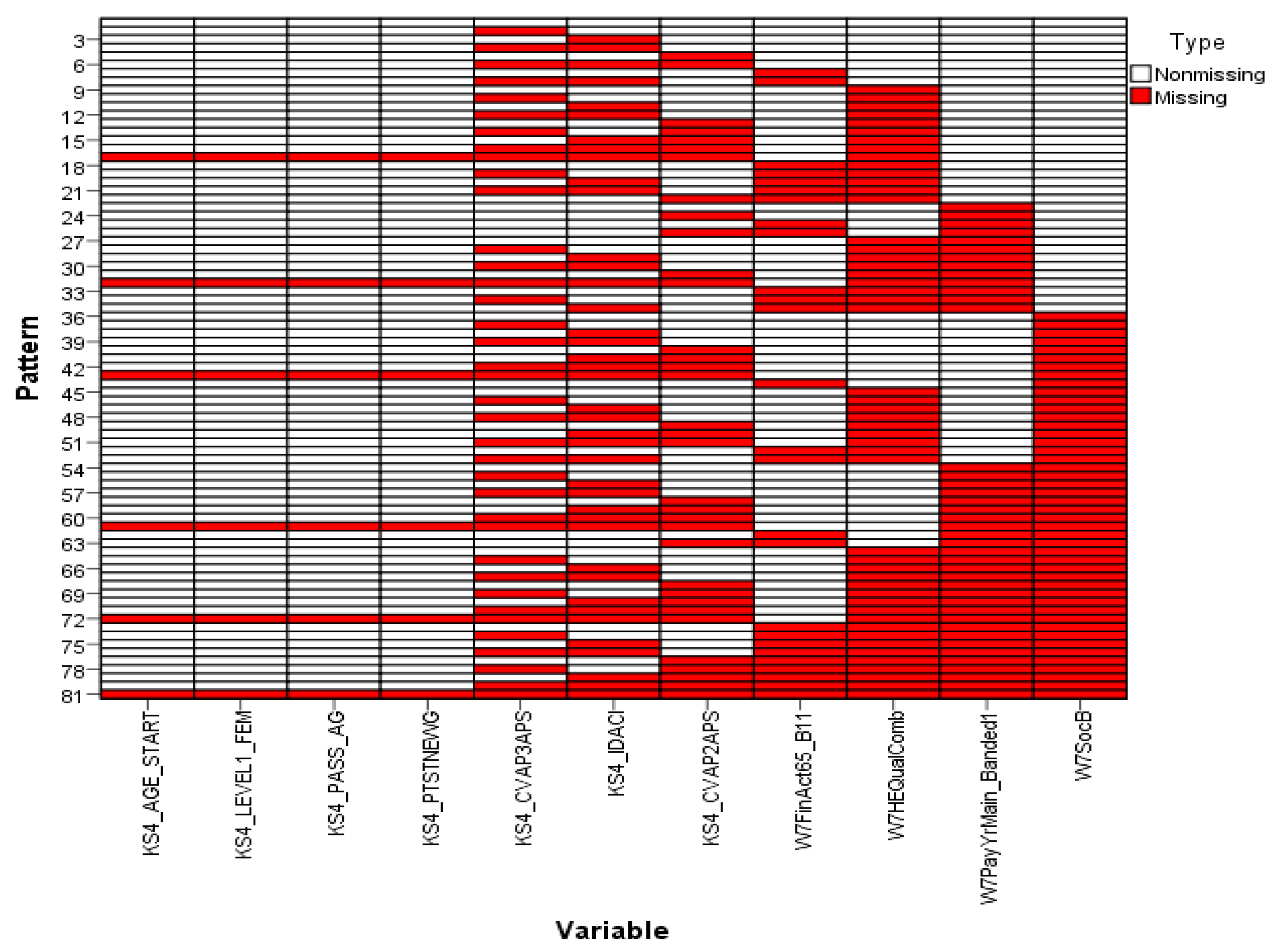
Analysing the missingness pattern showed that 100% of both the variables and the units were incomplete and only 30.12% of the values were missing. In general, the overall missingness pattern was identified using a chart. This chart comprises of a number of individual patterns on the vertical axis corresponding to the variables measured on the horizontal axis. Each individual pattern represents a group of units with the same pattern of incomplete and complete data across the variables. The chart orders the variables from left to right in increasing order of missing values. For example, pattern 6 in Figure 1 represents units that have missing values in the variables KS4_CVAP3APS, KS4_IDACI and KS4_CVAP2APS. The determination of the overall pattern of missingness depends, accordingly, on the grouping of missing and non-missing cells in the chart. If the data show a monotone missingness pattern, then all the missing cells and non-missing cells are contiguous. An arbitrary pattern shows clusters of missing and non-missing cells, as shown in Figure 1, across all charts [28] (Missing value patterns for the remaining variables are presented in Figure S1 in the Supplementary Materials). This makes it possible to argue that the missingness pattern of the entire dataset is also an arbitrary one. Accordingly, this result supports the choice of the Gibbs sampling technique, which is mainly used for arbitrary patterns of missing data.

The MI simulation process was executed $m=5$ times in parallel in order to produce five complete datasets using three iteration specifications, 25, 50 and 100, in order to test the convergence of the algorithm.

Table 1. Descriptive statistics for the observed data, the five imputed datasets and the five complete datasets.

	Observed Data	Imputed Datasets *			Complete Datasets *
Variable/iterations		25	50	100	25	50	100
KS4_IDACI
N	15,050.000	1072.000	1072.000	1072.000	16,122.000	16,122.000	16,122.000
Mean	0.247	0.255	0.253	0.252	0.248	0.248	0.248
St. Dev.	0.192	0.160	0.160	0.162	0.190	0.190	0.190
KS4_PASS_AG
N	15,758.000	364.000	364.000	364.000	16,122.000	16,122.000	16,122.000
Mean	9.116	7.838	7.638	7.609	9.087	9.083	9.082
St. Dev.	2.945	3.032	3.113	3.120	2.953	2.957	2.957
KS4_PTSTNEWG
N	15,758.000	364.000	364.000	364.000	16,122.000	16,122.000	16,122.000
Mean	358.959	277.748	271.099	272.080	357.126	356.976	356.998
St. Dev.	159.147	144.802	145.472	145.227	159.292	159.384	159.367
KS4_CVAP3APS
N	15,198.000	924.000	924.000	924.000	16,122.000	16,122.000	16,122.000
Mean	33.503	34.144	34.186	34.154	33.540	33.542	33.540
St. Dev.	6.755	8.010	8.057	8.047	6.835	6.838	6.837

Note: * The values represent the average, which is calculated for the five imputed/completed datasets. Variables definitions are included in Table S1 in the Supplementary Materials.

summarizes the descriptive statistics of a sub-sample of the 12 continuous variables imputed. The descriptive statistics for the remaining variables are presented in

Table A1. Descriptive statistics for the observed data, the five imputed datasets and the five complete datasets.

	Observed Data	Average of Imputed Datasets *			Average of Complete Datasets *
Variable/iterations		25	50	100	25	50	100
KS4_AGE_START
N	15,758.000	364.000	364.000	364.000	16,122.000	16,122.000	16,122.000
Mean	15.000	15.000	15.000	15.010	15.000	15.000	15.000
St. Dev.	0.063	0.060	0.060	0.060	0.060	0.063	0.060
KS4_CVAP2APS
N	14,911.000	1211.000	1211.000	1211.000	16,122.000	16,122.000	16,122.000
Mean	26.852	25.003	24.987	24.952	26.713	26.711	26.709
St. Dev.	4.117	4.674	4.683	4.687	4.190	4.191	4.192
W7PayYrMain_Banded1
N	4193.000	11,929.000	11,929.000	11,929.000	16,122.000	16,122.000	16,122.000
Mean	9094.920	9476.096	9538.915	9842.580	9376.960	9423.441	9648.129
St. Dev.	5539.053	4395.195	4456.949	4611.873	4725.416	4766.340	4881.393
W1GrssyrHH
N	6927.000	9195.000	9195.000	9195.000	16,122.000	16,122.000	16,122.000
Mean	31,166.263	34,473.754	34,726.024	34,468.330	33,052.653	33,196.532	33,049.559
St. Dev.	31,250.830	25,842.917	26,038.670	25,898.230	28,341.062	28,450.424	28,368.798
W2GrssyrHH
N	7612.000	8510.000	8510.000	8510.000	16,122.000	16,122.000	16,122.000
Mean	34,311.852	30,114.079	30,274.178	29,907.481	32,096.057	32,180.565	31,987.004
St. Dev.	30,424.576	23,421.468	23,318.433	23,281.929	27,041.356	26,987.403	26,983.425
W2BenTotBand1
N	13,047.000	3075.000	3075.000	3075.000	16,122.000	16,122.000	16,122.000
Mean	4689.964	6322.914	6584.429	6547.351	5001.422	5051.301	5044.229
St. Dev.	5279.402	4054.574	4125.593	4126.171	5113.919	5136.395	5135.268
W1yschat1
N	15,196.000	926.000	926.000	926.000	16,122.000	16,122.000	16,122.000
Mean	34.046	32.414	32.671	32.919	33.952	33.967	33.981
St. Dev.	7.302	7.268	7.197	7.084	7.310	7.303	7.294
W2yschat1
N	13,165.000	2957.000	2957.000	2957.000	16,122.000	16,122.000	16,122.000
Mean	32.395	30.813	31.167	31.406	32.105	32.170	32.214
St. Dev.	7.603	7.842	7.756	7.749	7.675	7.659	7.642

Note: * The average was calculated for the five imputed/completed datasets.

in Appendix A.

4. Discussion

To assess the convergence of the algorithm, plots of the means and standard deviations of the five imputed datasets plotted by iteration and imputation were used [13]. If the Gibbs sampler algorithm converges quickly, the series should indicate no pattern with no long upward or downward trends. The plots of the estimated parameters of the variables shown in Figure 2 show that the algorithm did converge with 25 iterations and that the convergence was smoother as the number of iterations increased to 50 and 100. As can be observed, the two variables measuring the KS4 results, KS4_PASS_AG and KS4_PTSTNEWG, did not converge with 25 iterations, but instead converged with 50 iterations and even showed smoother convergence with 100 iterations (The convergence plots for the remaining variables are presented in Figure S2 in the Supplementary Materials).

Given the complexity of the imputation models, it is important to employ diagnostics tests by comparing the observed and imputed data to help assess how reasonable are the imputation models employed. Graphic and numeric diagnostics could be used [29].

Methods of graphic diagnosis, such as density plots, could be helpful first diagnostics for discrepancies between observed to imputed values. Using Kernel density plots [29] the results in Figure 3 show that the observed and imputed values are not exactly similar where the imputed values could be higher than the observed values, such as in (KS4_IDACI) or lower (KS4_PASS_AG). The Kernel density plots for the rest of the variables are presented in Figure S3 in the Supplementary Materials. Similar findings were found in previous studies that used MI to impute missing values in children’s mental health datasets [30]. This could be attributed to the percentage of missing values (7% in the former and 2% in the latter) or the difference in the cases with missing values for the relevant variables or possible outliers in certain variables, especially the variables measuring income and financial benefits levels. As such, it is useful to observe numeric diagnostics as well.

Numeric diagnostics could be implemented by examining the differences between observed, imputed and complete datasets. For example, three points can be concluded about the differences between the observed data, the five imputed datasets and the five complete datasets in Table 1 and Table A1. First, there are few differences between the statistics of the observed data and the five complete datasets. Second, there are also very minimal differences between the statistics of the five complete datasets over the three iterations specifications. Third, this also holds for the five imputed datasets.

Another approach is to use the Kolmogorov–Smirnov test to compare the observed and imputed values, where any significant differences between the p-values of the observed and the imputed values raise a concern [29]. In this analysis, the pooled imputed p-values were used. The pooled p-values are calculated using the mean of the p-values for the five imputed values. Using the conventional cut-off point of 0.05 [29], the results show that only KS4_AGE_START and KS4_PTSTNEWG showed a discrepancy between the observed and imputed values. The KS test results are presented for 10%, 5% and 1% significance levels in Table S2 in the Supplementary Materials. The results were consistent for 1% and 10% significance levels. The results were also consistent with the results of other studies that used the KS test as a diagnostic check of multiple imputed data from a simulation study [31].

Another form of numeric diagnostics examines the differences between observed and imputed data. Specifically, (1) an absolute difference in the means between the observed and imputed values greater than two standard deviations, or (2) a ratio of variances of the imputed and observed data that is less than 0.5 and greater than 2 could raise a flag for variables of concern [30]. The results showed that the absolute differences in the means were acceptable for five of the twelve continuous variables, while none of the variables raise any concerns for the variance ratio criterion. In the Supplementary Materials, the absolute differences in the means are presented in Table S3 and the ratios of the variances are presented in Table S4. This is in line with the findings of the same diagnostics tests of previous studies [30], proving the validity of the diagnostics.

Conventional tests of variances and means differences, such as the F-test and t-test, could be used as well [31]. However, testing of the means difference between the observed and pooled imputed values showed that there were discrepancies between the two rejecting the test at 10%, 5% and 1% significance levels. The p-values of the t-tests of the means differences between the observed and pooled imputed values are presented in Table S5 in the Supplementary Materials. Independent t-tests for the means difference between the observed values and each of the five imputed set of values also showed discrepancies for the three iteration configurations for the examined variables aside from five variables; KS4_AGE_START, KS4_IDACI, KS4_CVAP3APS, W7PayYrMain_Banded1 (25 iterations only) and W2yschat1. In addition, the F-test results for the variances difference also showed discrepancies for half of variables aside from KS4_AGE_START, KS4_PTSTNEWG, W1GrssyrHH, W1yschat1, W2yschat1 and W2BenTotBand1 (25 iterations only) (The t-tests and F-tests p-values are presented in Table S6 in the Supplementary Materials). However, these discrepancies could be attributed to the difference in the sample size of the two sets of values for every variable given the percentage of missing data. They could also be attributed to the existence of outliers in certain variables, especially those measuring income, such as W1GrssyrHH and W1GrssyrHH, or the level of benefits received W2BenTotBand1.

It is important to note that in general, flagged discrepancies between observed and imputed data do not necessarily signal a problem. Consistent with existing studies [29] the findings of this paper show that there are no foolproof tests of the assumptions of the imputation procedure. However, under MAR, it is not expected that the imputed values should resemble the observed ones. The MI can help recover these differences based on information in the observed data [31]. The FCS-MCMC simulation technique was used and analysed in a number of previous studies. However, with the existence of other MCMC simulation methods, such as data augmentation and the Metropolis–Hastings algorithm, a comparison of the results of these imputation methods on the dataset used in this paper would be of significant research interest.

5. Conclusions

Given the uncertainty of missing data, multiple imputation is known to be superior to other imputation techniques as it accounts for this uncertainty. This paper contributes to a number of avenues in the literature on the economics of education and applied statistics by reviewing the theoretical foundation of missing data analysis with a special focus on the application of multiple imputation to longitudinal educational longitudinal. Earlier attempts to use MCMC simulation were applied on relatively small datasets with small numbers of variables. Therefore, another contribution of the paper is its application and comparison of the imputation technique on a large longitudinal English educational study for three iteration specifications. This paper employed MI on a large educational longitudinal study using using a fully conditional specification method based on an iterative Markov Chain Monte Carlo (MCMC) simulation using a Gibbs sampler algorithm. The results show that the missingness pattern of the entire dataset is an arbitrary one. Accordingly, this result supports the choice of the Gibbs sampling technique. The plots of the estimated parameters of the variables show that the algorithm did converge with 25 iterations and that the convergence was smoother as the number of iterations increased to 50 and 100.

This paper used both graphical and numeric diagnostics checks of verify the accuracy of the imputation. These results are consistent with previous studies that employed MI and these diagnostics checks to verify the accuracy of the imputation [29,30,31]. Kernel density plots showed that the observed and imputed values were not exactly similar where the imputed values could be higher than the observed values, suggesting the need for numeric tests. Consistent with other studies [31], the KS test results showed that the majority of the variables did not show a discrepancy between the observed and imputed values. The results also showed that the absolute differences in the means were acceptable for five of the twelve continuous variables, while none of the variables raised any concerns over the variance ratio criterion [30]. However, conventional tests of variances and means differences, such as F-test and t-test, showed discrepancies between the observed and imputed data. It is important to note that in general, flagged discrepancies between observed and imputed data do not necessarily signal a problem. Existing studies show that there are no foolproof tests of the assumptions of the imputation procedure [29].

It can be argued that although there is no consensus over the results of all the diagnostics checks, most of the results suggest that the proposed multiple imputation method was efficient at imputing missing data. Additionally, the results of the simulation proved the convergence of the algorithm. The final output of the application generated a longitudinal complete dataset that will enable researchers in the field to estimate educational production functions more appropriately, avoiding estimation bias.