Abstract
In many industries and plants, a stable power supply system with acceptable cost/benefit is essential. This paper investigates the cost-effectiveness of an unreliable retrial system that includes standby generators and experiences the switchover failures of standby generators. Four different standby retrial configurations are included, and each configuration includes various numbers of primary and standby generators. Upon arrival, a failed generator is repaired immediately if the server is available; otherwise, the failed generator will enter into orbit. The server is subject to breakdown even when the server is idle. The explicit expressions of the mean time-to-failure and steady-state availability for each configuration are derived and compared. We also compare the cost/benefit ratio among four configurations. The developed results can provide managers with decision reference for stable power supply system and cost reduction.
1. Introduction
A robust power supply system with acceptable cost/benefit is a fundamental part for high-tech fabrication plants (called fabs), which plays an important role in modern industries, such as packaging and testing, IC design, and wafer foundry. For fabs, a stable power supply system is essential for maintaining the competition. Liu et al. [1] applied a retrial system with standby switching failure to model the power supply system for a fab. In their work, the repair server is assumed to be reliable. They applied the supplementary variables techniques to obtain the explicit expressions of the steady-state availability. However, in real world application, the repair server may be malfunctioned, but can be repaired. To address this issue, in this paper, we extend the work of Liu et al. [1] to the case of a unreliable repair server. As we know, the more system features we take into consideration simultaneously, the more difficulty we have in modelling the system and deriving the equations. Hence, the investigated model has not been studied in the literature so far. In addition, we derive the explicit expressions of the mean time-to-failure and steady-state availability for each configuration. Four different standby retrial configurations are included, and each configuration includes various numbers of primary and standby generators. Except for obtaining the explicit expressions of steady-state availability for each configuration, we also obtain the explicit expressions of the mean time-to-failure for each configuration and make a comparison.
Due to the practical applicability of the retrial queues, more and more researchers have attracted attention to retrial systems. For existing works related to retrial systems, interested readers can refer to Falin and Templeton [2], Artalejo [3], Artalejo and Gomez-Corral [4], Yang and Chang [5], Chen [6], Chen and Wang [7], Yang and Tsao [8], Phung-Duc [9], and the references therein. Recently, Yen, Wang, and Wu [10] investigated the system availability and sensitivity analysis of a retrial queue with working breakdowns operating under the F-policy. Yen and Wang [11] investigated the reliability and availability of four retrial systems with imperfect coverage and compared the cost/benefit among these four retrial systems. Gao and Wang [12] studied a retrial unreliable machine system with mixed standbys and optimized the cost-effectiveness ratio. Wu and Yang [13] constructed a repairable system with warm standbys and imperfect switchovers and evaluated its availability and reliability. Hirata et al. [14] presented an evaluation method for the variance of failure times in the two-component priority standby redundant system by expanding the idea by evaluating mean time-to-failure proposed in the previous research. They proposed a procedure for deriving the reliability function in the system based on the maximum entropy principle by utilizing mean time-to-failure and variance of failure times. Liu et al. [15] studied a K-out-of-N retrial system with mixed standby components and a single repair server under Bernoulli vacation schedule. They used vector Markov process and Laplace transform theory to derive the steady-state availability, reliability function, and mean time-to-failure.
The process of switching over standbys in the actual repairable standby system may not be perfect, as described by Lewis [16]. Kuo and Ke [17] constructed three standby unreliable systems with switching failure and compared the cost/benefit ratio and availability among the three systems. Ke et al. [18] modeled a machine repairing system incorporating standby switching failure, in which the general repair times are considered, and constructed a cost function to search the optimal system parameters. Utilizing supplementary variables, Lee [19] studied the availability analysis of a redundancy model with general repair times, switching failure, and interrupted repairs. Other research works along this line includes Shekhar et al. [20], Ke et al. [21], Jain and Gupta [22], and Liu et al. [23].
The contents of this work are managed in the following sections. The model description is given in Section 2. The four different unreliable retrial systems are introduced in Section 3. For each configuration, the explicit expressions for mean time-to-failure (MTTF) and steady-state availability (Av) are derived by the matrix-analytic method. The numerical results are presented in Section 4. We also rank four configurations according to MTTF, Av, and the cost/benefit ratio. Section 5 is devoted to the summary and conclusions.
2. System Description
By referring to Liu et al. [1], we consider that a system requires 24 megawatts (MW) power and assume that the power generating capacity of a generator is available in units of 24 MW, 12 MW, and 8 MW. In this system, the energy generator that is supplying electricity is called the primary generator, and the energy generator that is online but does not provide power is called the standby generator. Both the primary and standby energy generators may fail and can be repaired. The failure times of primary and standby generators obey an exponential distribution with rate λ and α (0 < α < λ), respectively. We assume that the switching device has a failure probability q. In the repair facility, only one server is responsible for repairing a failed generator and there is no waiting space in front of the server. Hence, a failed generator finding that the server is free is repaired immediately; otherwise, it will enter orbit. The retrial time obeys exponential distribution with the rate γ. The failed generators will continue to retry until it gets the required repair. The repair times of a failed generator obey exponentially distributed with rate µ. Additionally, the server may fail at any time even if it is idle. The server fails with an exponential breakdown rate of η. The repair time for the server obeys exponentially distributed with mean β−1.
Four configurations are considered as follows: configuration 1 consists of one 24 MW primary generator and one 24 MW standby generator. Configuration 2 includes two 12 MW primary generator s and one 12 MW standby generator. Configuration 3 contains two 12 MW primary generators and two 12 MW standby generators. Configuration 4 contains three 8 MW primary generators and two 8 MW standby generators.
3. Systematic Methodology
We first draw the transition-rate diagram for each configuration. According to the diagram, we develop the differential-difference equations. Finally, we utilize the matrix-analytic method to obtain the explicit expressions of MTTF and Av. We define the following probabilities throughout the paper.
where represents the number of failed generators in orbit at time t, and denotes the states of the server at time t, and
3.1. Configuration 1
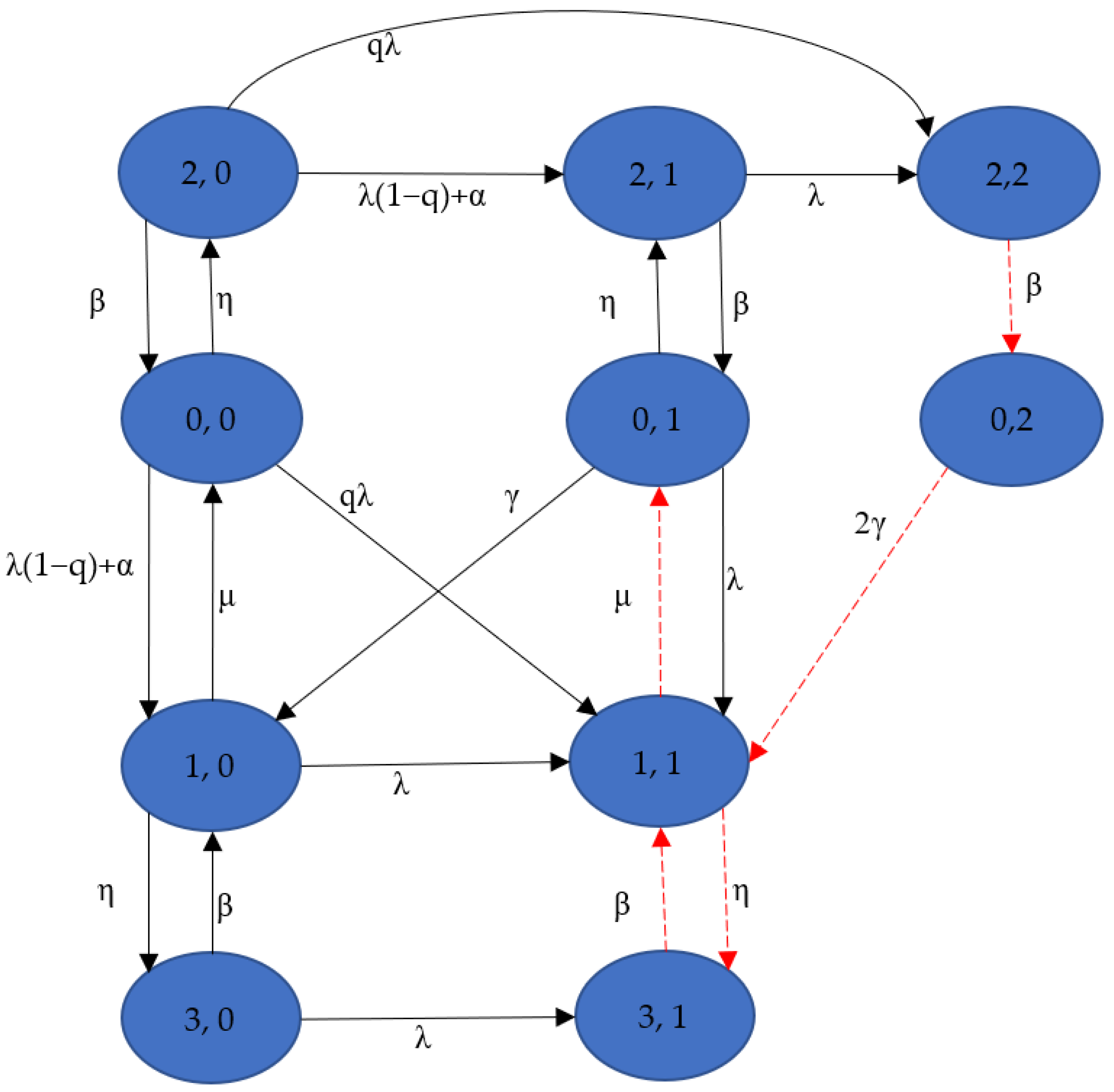
For the reliability case, the state-transition-rate diagram of configuration 1 is provided in Figure 1. It is assumed that the system is characterized as a failure as soon as the remaining electricity generation capacity is less than 24 MW. So, if the system cannot be resumed, the states (0, 2), (1, 1), (2, 2), and (3, 1) are absorbing states. Based on the Figure 1, the differential-difference equations can be written as the following matrix form:
where

Figure 1.
State-transition-rate diagram of configuration 1.
To evaluate MTTF1, we define A1 as the transpose matrix of Q1 omitting the row and column for the absorbing states. First, 1 represents a column vector with all elements equal to 1, and the initial condition is
Then, we can obtain
where
MTTF1 can be expressed as
Due to the complexity of the explicit expression for MTTF1, this formula is difficult to display here. However, by using a suitable computer program, it can be evaluated numerically.
To discuss the availability of this configuration, we need the process below to obtain the steady-state availability. In steady-state, we let the derivatives of the state probabilities be zero. Then, we have
By partitioning the probability vector as , where and , then Equation (4) can be rewritten as
where
and 0 is a zero matrix with the appropriate dimension.
By solving Equation (5) and after some routine substitutions, we have
Hence, we can calculate by solving Equation (9) and the normalizing condition . Thus, the steady-state availability of configuration, , can be computed once the steady-state probabilities are obtained.
3.2. Configuration 2
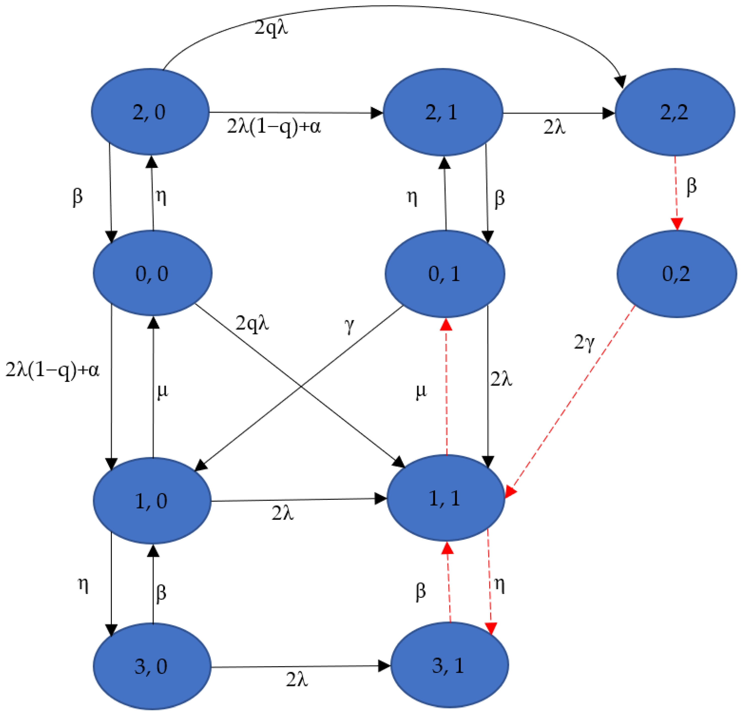
Figure 2 presents the state-transition-rate diagram of configuration 2. Similarly, the transition from (2, 2) to (0, 2), the transition from (0, 2) to (1, 1), the transition from state (1, 1) to (0, 1) and (3, 1), and the transition from (3, 1) to (1, 1) are ignored when investigating the system MTTF. The associated probability vector for this configuration is defined as:

Figure 2.
State-transition-rate diagram of configuration 2.
We can write the differential-difference equations of configuration 2 as the following matrix form:
where
We define A2 as the transpose matrix of Q2 omitting the row and column for the absorbing state. Let
represent the initial condition. We can obtain
where
For this configuration, MTTF2 can be expressed as
As mentioned earlier, the explicit expression of MTTF2 is not shown here due to its complexity. We compare the four configurations in Section 4 based on the calculated numerical results. We utilize the same process in the prior subsection to get the steady-state availability. In steady-state, we let the derivatives of the state probabilities be zero, then
Solving the above equation and using the normalizing condition , we can obtain the steady-state probabilities. Once the steady-state probabilities are obtained, the availability of configuration 2, , can be computed.
3.3. Configuration 3
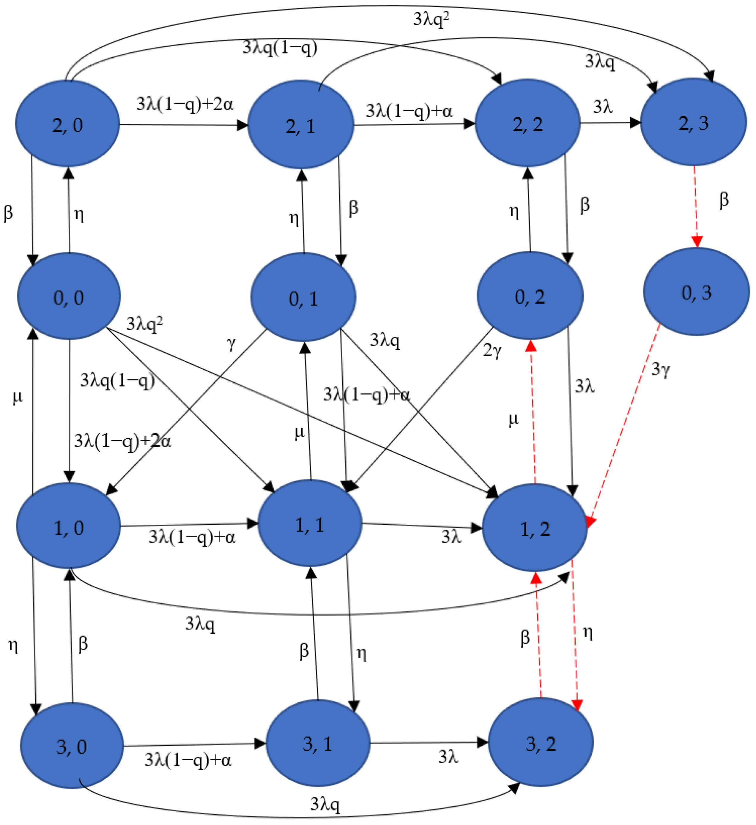
Figure 3 presents the state-transition-rate diagram of configuration 3. When deriving the system MTTF, the transition from state (2, 3) to (0, 3), transition (0, 3) to (1, 2), transition from state (1, 2) to states (0, 2) and (3, 2), and transition from state (3, 2) to (1, 2) should be deleted. Let
represent the initial condition. We can write the differential-difference equations of this configuration as the following matrix form:
where

Figure 3.
State-transition-rate diagram of configuration 3.
We define A3 as the transpose matrix of Q3 omitting the row and column for the absorbing state. After the transpose operation, we have
We can obtain the mean time-to-failure for configuration 3 as follows.
For the availability case of this configuration, we utilize the same process in the prior subsection to get the steady-state availability. In steady-state, we let the derivatives of the state probabilities be zero, then we have
where
Similarly, solving Equation (17) recursively with the normalizing condition can obtain the steady-state probabilities. Once the steady-state probabilities are obtained, then the availability of this configuration, is computed.
3.4. Configuration 4
The state-transition-rate diagram of configuration 4 is shown in Figure 4. The associated probability vector is

Figure 4.
State-transition-rate diagram of the configuration 4.
According to the Figure 4, the differential-difference equations of this configuration can be written as the following matrix form:
where
We define A4 as the transpose matrix of Q4 omitting the row and column for the absorbing state. Let
represent the initial condition, we can obtain
where
We utilize the same process in the prior subsection to get the steady-state availability. The steady-state probabilities can be obtained by solving
with the normalizing condition , where
Once the steady-state probabilities are obtained, the availability of configuration 4, , is computed. In the following section, we compare these four configurations based on MTTF and the availability.
4. Comparative Results
4.1. Comparison of MTTF and Av
The cases listed below are provided in this section to compare four configurations according to their MTTFi and Avi (i = 1,2,3,4).
- Case1.
- Given , , , , , , and change the values of .
- Case2.
- Given , , , , , , and change the values of .
- Case3.
- Given , , , , , , and change the values of .
- Case4.
- Given , , , , , , and change the values of .
- Case5.
- Given , , , , , , and change the values of .
- Case6.
- Given , , , , , , and change the values of .
Table 1 and Table 2 show the results of MTTF and Av for each configuration. From Table 1, the MTTF of configuration 3 is larger than that of configurations 1, 2, and 4 if , but the MTTF1 is larger than that of the other configurations if . From Table 2, one can find that based on the comparison of , configuration 3 may be the best configuration as , but as , the best configuration may be configuration 1. In addition, no matter how we vary the values of , , , and , the best configuration is always configuration 1 whether it is based on MTTF comparisons or comparisons. From Table 2, one can find that in most cases, configuration 1 has the highest steady-state availability, while configuration 4 performs the worst among the four configurations, only outperforming configuration 2 in some cases. As a standard for comparing these four configurations, the cost/benefit ratio may be equitable to the benefit, since each configuration spends different costs during the construction process.

Table 1.
Comparisons of configurations 1–4 for MTTF.
Table 2.
Comparisons of configurations 1–4 for .
4.2. Comparison Based on Their Cost/Benefit Ratio
We consider a situation where different configurations may have different costs. To compare different configurations fairly, these costs should be considered. We list the costs (Ci) for each configuration i (i = 1,2,3,4) as shown below.
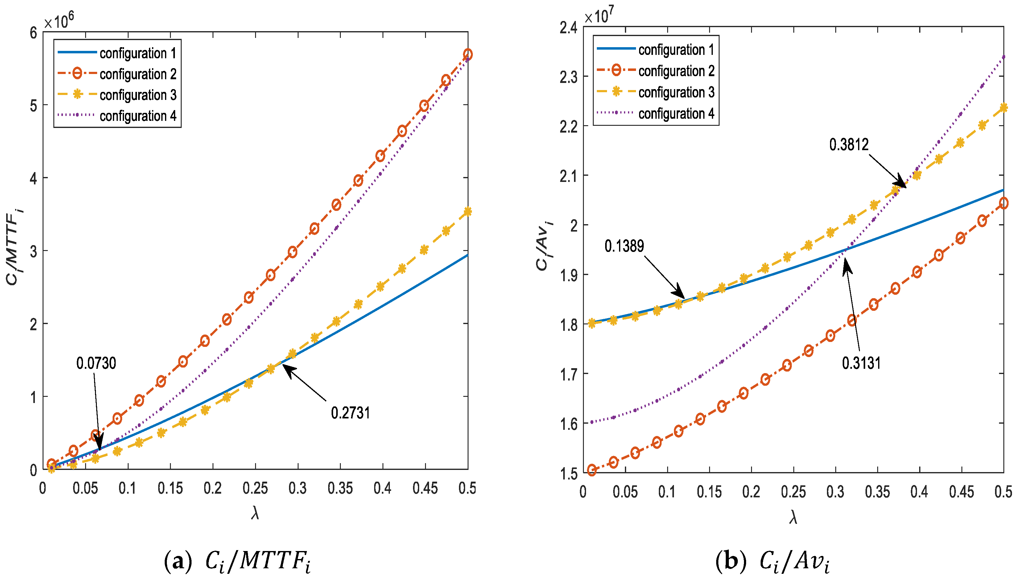
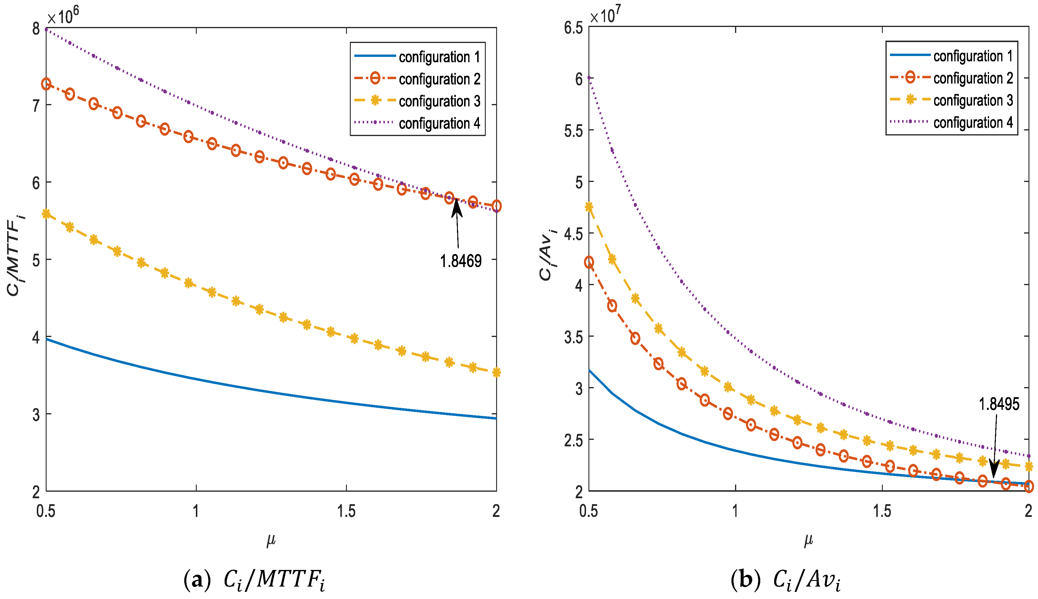
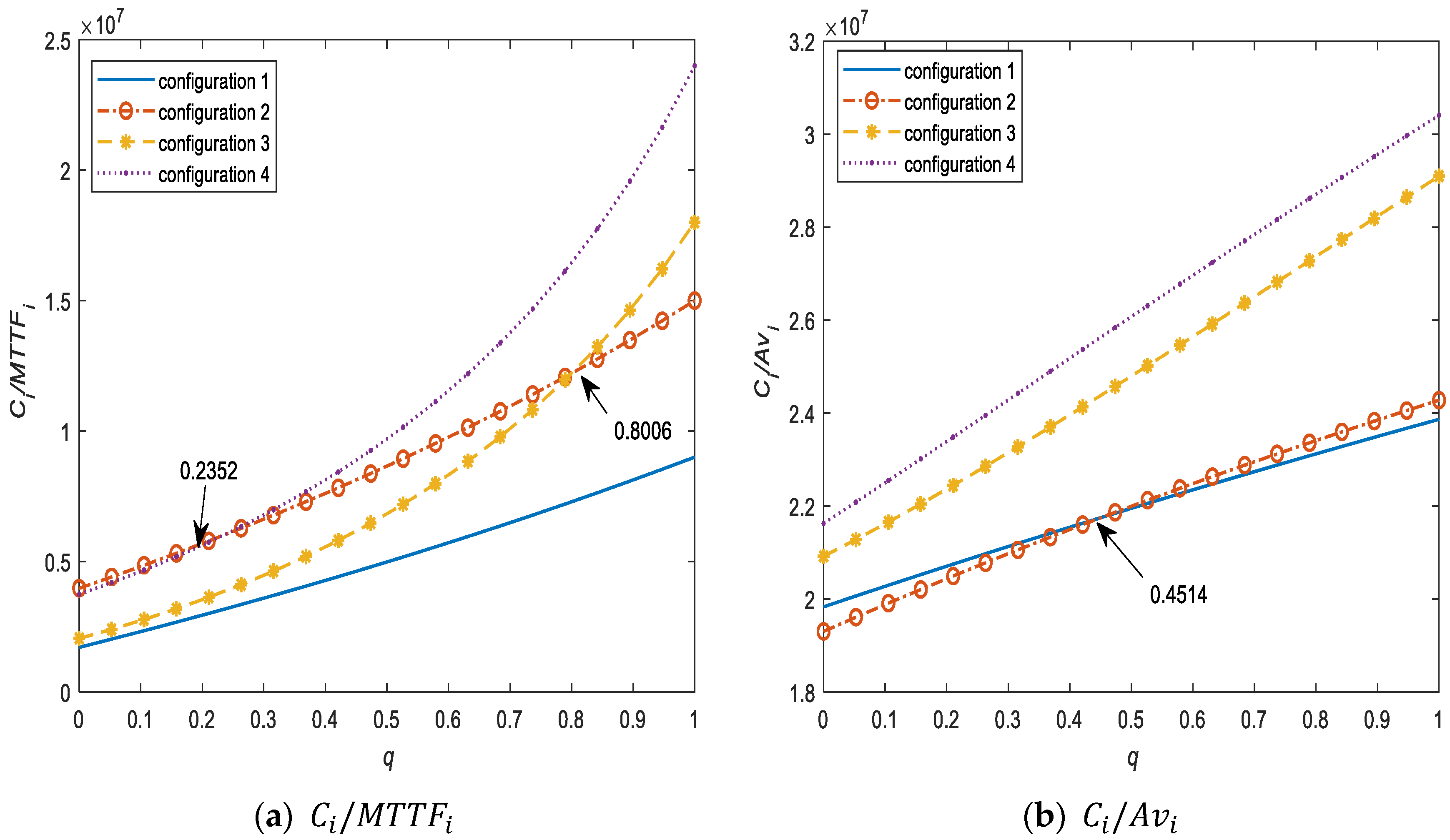
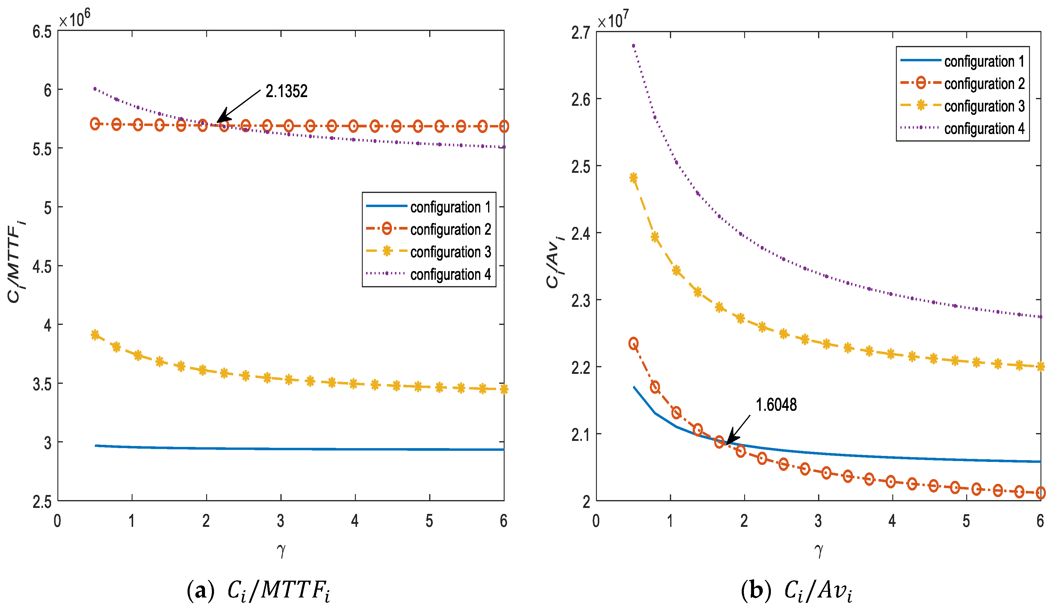
Considering the same cases as in the previous subsection, we compare the ratio for each configuration i (i = 1,2,3,4), i.e., and . The results depicted in Figure 5, Figure 6, Figure 7, Figure 8, Figure 9 and Figure 10 indicate that when , , or increase, and increase for any configuration, but and decrease as , or increase for any configuration. Figure 5 displays that configuration 2 has minimum for different ranges of . The best configuration of ratio is if . Otherwise, the best configuration of ratio is . The worst configuration of ratio is .

Figure 5.
versus .

Figure 6.
versus .
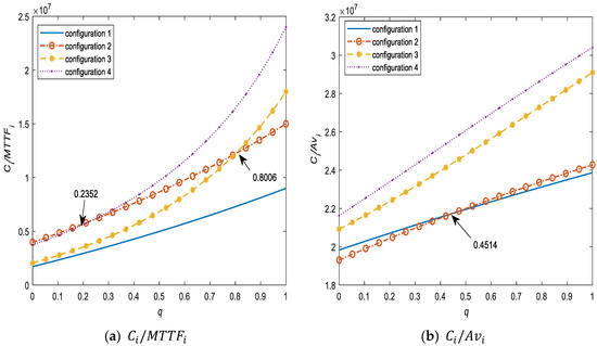
Figure 7.
versus .
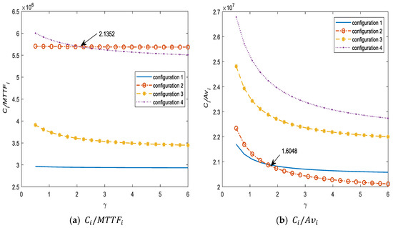
Figure 8.
versus .
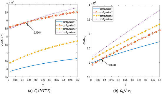
Figure 9.
versus .
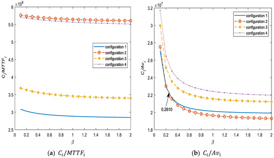
Figure 10.
versus .
From Figure 6, Figure 7, Figure 8, Figure 9 and Figure 10, the optimum configuration based on the is dependent on , , , , and . With the ratio, the worst configuration is configuration 4 for different ranges of , , , , and . has the minimum ratio if , , or . Otherwise, the best configuration of the is . In addition, they also show that the optimum configuration based on the will not change as , , , and vary. has the minimum ratio. The worst configuration of ratio is for all ranges of . The worst configuration is if , , or . Otherwise, the worst configuration is configuration 4.
5. Conclusions
This work evaluated the cost-benefit of four standby unreliable retrial configurations with standby switching failure. The explicit and computationally tractable expressions for MTTFi and () were derived for each configuration. A Matlab computer program is utilized to carry out the proposed approach. We ranked four configurations based on , and the cost/benefit ratio. According to our numerical results, the system with configuration 1 displayed the highest performance in most cases. Therefore, the procedure proposed in this paper can provide managers with a valuable tool to select the configuration with greatest benefit in terms of MTTF or availability. For future research, we may consider the general repair times of failed generators and the server. Moreover, we may also design the optimal management system.
Author Contributions
Conceptualization, T.-H.L., Y.-L.H., Y.-B.L. and F.-M.C.; writing—original draft preparation, T.-H.L.; writing—review and editing, Y.-L.H. and F.-M.C.; supervision, Y.-B.L. and F.-M.C. All authors have read and agreed to the published version of the manuscript.
Funding
This research was partially funded by Ministry of Science and Technology of Taiwan under grants MOST 109-2221-E-324-013.
Institutional Review Board Statement
Not applicable.
Informed Consent Statement
Not applicable.
Data Availability Statement
Not applicable.
Acknowledgments
The authors thank the editor and the anonymous referees for the valuable comments and suggestions, which significantly improved the quality of the paper.
Conflicts of Interest
The authors declare no conflict of interest. The funders had no role in the design of the study; in the collection, analyses, or interpretation of data; in the writing of the manuscript, or in the decision to publish the results.
References
- Liu, T.H.; Wang, C.M.; Lin, Y.B.; Chang, F.M. Evaluation of the cost-benefit of standby retrial systems incorporating switching failure and general repair times. Int. J. Appl. Sci. Eng. 2021, 18, 2021213. [Google Scholar] [CrossRef]
- Falin, G.; Templeton, J. Retrial Queues; Chapman & Hall: London, UK, 1997. [Google Scholar]
- Artalejo, J.R. Accessible bibliography on retrial queues: Progress in 2000–2009. Math. Comput. Model. 2010, 51, 1071–1081. [Google Scholar] [CrossRef]
- Artalejo, J.R.; Gomez-Corral, A. Retrial Queueing Systems: A Computational Approach; Springer: Berlin/Heidelberg, Germany, 2008. [Google Scholar]
- Yang, D.Y.; Chang, Y.D. Sensitivity analysis of the machine repair problem with general repeated attempts. Int. J. Comput. Math. 2018, 95, 1761–1774. [Google Scholar] [CrossRef]
- Chen, W.L. System reliability analysis of retrial machine repair systems with warm standbys and a single server of working breakdown and recovery policy. Syst. Eng. 2018, 21, 59–69. [Google Scholar] [CrossRef]
- Chen, W.L.; Wang, K.H. Reliability analysis of a retrial machine repair problem with standbys and a single server with N-policy. Reliab. Eng. Syst. Saf. 2018, 180, 476–486. [Google Scholar] [CrossRef]
- Yang, D.Y.; Tsao, C.L. Reliability and availability analysis of standby systems with working vacations and retrial of failed components. Reliab. Eng. Syst. Saf. 2019, 182, 46–55. [Google Scholar] [CrossRef]
- Phung-Duc, T. Retrial queueing models: A survey on theory and applications. arXiv 2019, arXiv:1906.09560. [Google Scholar]
- Yen, T.C.; Wang, K.H.; Wu, C.H. Reliability-based measure of a retrial machine repair problem with working breakdowns under the F-policy. Comput. Ind. Eng. 2020, 150, 106885. [Google Scholar] [CrossRef] [PubMed]
- Yen, T.C.; Wang, K.H. Cost benefit analysis of four retrial systems with warm standby units and imperfect coverage. Reliab. Eng. Syst. Saf. 2020, 202, 107006. [Google Scholar] [CrossRef]
- Gao, S.; Wang, J. Reliability and availability analysis of a retrial system with mixed standbys and an unreliable repair facility. Reliab. Eng. Syst. Saf. 2021, 205, 107240. [Google Scholar] [CrossRef]
- Wu, C.H.; Yang, D.Y. Dynamic control of a machine repair problem with switching failure and unreliable repairmen. Arab. J. Sci. Eng. 2020, 45, 2219–2234. [Google Scholar] [CrossRef]
- Hirata, R.; Arizono, I.; Takemoto, Y. On reliability analysis in priority standby redundant systems based on maximum entropy principle. Qual. Technol. Quant. Manag. 2021, 18, 117–133. [Google Scholar] [CrossRef]
- Liu, S.; Hu, L.; Liu, Z.; Wang, Y. Reliability of a retrial system with mixed standby components and Bernoulli vacation. Qual. Technol. Quant. Manag. 2021, 18, 248–265. [Google Scholar] [CrossRef]
- Lewis, E.E. Introduction to Reliability Engineering, 2nd ed.; Wiley: New York, NY, USA, 1996. [Google Scholar]
- Kuo, C.C.; Ke, J.C. Comparative analysis of standby systems with unreliable server and switching failure. Reliab. Eng. Syst. Saf. 2016, 145, 74–82. [Google Scholar] [CrossRef]
- Ke, J.C.; Liu, T.H.; Yang, D.Y. Machine repairing systems with standby switching failure. Comput. Ind. Eng. 2016, 99, 223–228. [Google Scholar] [CrossRef]
- Lee, Y. Availability analysis of redundancy model with generally distributed repair time, imperfect switchover, and interrupted repair. Electron. Lett. 2016, 52, 1851–1853. [Google Scholar] [CrossRef]
- Shekhar, C.; Jain, M.; Raina, A.A.; Mishra, R.P. Sensitivity analysis of repairable redundant system with switching failure and geometric reneging. Decis. Sci. Lett. 2017, 6, 337–350. [Google Scholar]
- Ke, J.C.; Liu, T.H.; Yang, D.Y. Modeling of machine interference problem with unreliable repairman and standbys imperfect switchover. Reliab. Eng. Syst. Saf. 2018, 174, 12–18. [Google Scholar] [CrossRef]
- Jain, M.; Gupta, R. N-policy for redundant repairable system with multiple types of warm standbys with switching failure and vacation. Int. J. Math. Oper. 2018, 13, 419–449. [Google Scholar] [CrossRef]
- Liu, T.H.; Ke, J.C.; Kuo, C.C. Machine interference problem involving unsuccessful switchover for a group of repairable servers with vacations. J. Ind. Manag. Optim. 2021, 17, 1411–1422. [Google Scholar] [CrossRef] [Green Version]


Publisher’s Note: MDPI stays neutral with regard to jurisdictional claims in published maps and institutional affiliations. |
© 2022 by the authors. Licensee MDPI, Basel, Switzerland. This article is an open access article distributed under the terms and conditions of the Creative Commons Attribution (CC BY) license (https://creativecommons.org/licenses/by/4.0/).