Why Stable Finite-Difference Schemes Can Converge to Different Solutions: Analysis for the Generalized Hopf Equation

Abstract

The example of two families of finite-difference schemes shows that, in general, the numerical solution of the Riemann problem for the generalized Hopf equation depends on the finite-difference scheme. The numerical solution may differ both quantitatively and qualitatively. The reason for this is the nonuniqueness of the solution to the Riemann problem for the generalized Hopf equation. The numerical solution is unique in the case of a flow function with two inflection points if artificial dissipation and dispersion are introduced, i.e., the generalized Korteweg–de Vries-Burgers equation is considered. We propose a method for selecting coefficients of dissipation and dispersion. The method makes it possible to obtain a physically justified unique numerical solution. This solution is independent of the difference scheme.

1. Introduction

Propagation of nonlinear waves in continuous media can lead to the formation of thin layers with high gradients of the main flow parameters. The flow parameters change significantly only on large scales outside such thin layers. The appearance of high-gradient zones is a property of the solution, which is embedded in the equations themselves and is not related to the existence of high-gradient zones at the initial time. For example, high-gradient zones appear in shock waves. The solution is continuous if the mathematical model describes the flow both on small (inside the high-gradient zone) and large scales. According to [1], we imply the solution, which represents a continuous change in values corresponding to the discontinuity as a discontinuity structure (shock profile). In relevant cases, numerical multiscale and multidimensional modeling of flows with shock waves requires high-performance computing systems, which do not currently exist.

Detailed models take into account the physical mechanisms that provide continuous changes in flow parameters in thin layers. In some cases, the detailed model is replaced by a simplified one. If shockwave flows are considered, simplified equations are the nonlinear hyperbolic equations. Hyperbolic equations arise as a limiting case if the scale of the thin shock layer becomes much smaller than that of a significant parameter change outside the thin layer.

Shock-capturing methods are based on the same algorithm in the entire calculation area, including regions of discontinuities. In this case, the discontinuities are smeared and have a structure. The effective width of the structure is determined by dissipation and dispersion of the difference scheme. Thus, the discontinuity is replaced by a thin layer of a few cells thick. The solution changes rapidly in this layer. The width of the profile is determined by the choice of a particular numerical scheme, namely the terms with higher-order derivatives in the differential approximation of the scheme.

If the Hugoniot locus has inflection points, the numerical solution of the Riemann problem depends on the difference scheme (see [2]). In [2], a model equation of state was used for gas with the Hugoniot locus having several inflection points. Different numerical solutions to the Riemann problem were obtained when the approximation order of the difference scheme was decreased from the second to the first.

Examples of the Hugoniot locus with several inflection points for metals are given in [3,4].

The paper [5] initiated the systematic elucidation of the notion of the generalized (weak) solution of quasilinear hyperbolic systems. Since [5] was released, it has been customary to primarily study solutions of the Hopf equation with complex nonlinearity. The study of reduced models often allows us to infer fundamental properties of the solution to the detailed problem. The generalized Hopf equation is a meaningful mathematical model in the sense of nonlinearity. It is one of the simplest reduced equations, which generates shock wave solutions that have been investigated for various flow functions. In [5,6,7], convex and concave-convex flow functions were studied under the assumption that only dissipative processes occur in the thin shock layer. Traveling-wave solutions in the case of the flow function with one inflection point were classified in [8,9,10].

The Riemann problem for the generalized Hopf equation in the case of a flow function with two inflection points was considered in [11]. It was shown [11] that there is a fundamental difference between the case when only dissipative processes are considered and when dispersive terms are included in addition to dissipative ones. The solution to the Riemann problem for the generalized Hopf equation is not unique when dissipation and dispersion exist, even if all discontinuities with structure are used to obtain the solution. Examples of non-unique solutions of self-similar problems for the generalized Hopf equation, considered to be a simplification of the generalized Korteweg–de Vries-Burgers (KdVB) equation, are given in [12]. In [11,12], the nonuniqueness of solutions is a consequence of the existence of special, or non-classical, discontinuities. The Lax condition [13] is violated for undercompressive discontinuities.

An analytical solution for an undercompressive discontinuity in the case of a modified KdVB equation with a cubic flow function was found in [14]. The interaction of dissipation-dispersion waves corresponding to discontinuities with the interface of two media with different dissipation and dispersion coefficients was considered in [15,16,17].

Traveling-wave solutions of the KdVB equation were considered in [17] for the case when the dissipation coefficient $\mu$ is a function of the coordinate and time. Some external influence causes the change in the dissipation coefficient. Linear instability of obtained traveling-wave solutions was studied in [18].

Discontinuous solutions of the generalized Hopf equation with a flow function with four inflection points were studied in [19] under the assumption that the continuous and strong change in medium parameters in thin shock layers is described by the generalized Korteweg–de Vries-Burgers equation.

The present paper shows why different numerical methods give different solutions and why choosing the correct solution a priori is only possible with information about the processes occurring inside the thin shock layer. The paper proposes a method for adapting any convergent difference scheme. Due to this method, all numerical solutions of the Riemann problem converge to the unique solution, which does not depend on the difference scheme.

The paper is organized as follows. In Section 2, we formulate the Riemann problem for Equation (1). Next, in Section 3, a family of nonconservative difference schemes is constructed. Calculations are made for various scheme parameters. In Section 4, the family of conservative schemes and obtained solutions are discussed. In Section 5 and Section 6, we analyze these obtained solutions. Conditions on artificial viscosity and dispersion coefficients are formulated to obtain a unique and physically reasonable solution to the Riemann problem. The main conclusions are formulated in Section 7.

2. The Riemann Problem for the Generalized Hopf Equation

The generalized Hopf equation

$$\frac{\partial v}{\partial t}+\frac{\partial \varphi \left(v\right)}{\partial x}=0,v=v(x,t),$$

(1)

is the scalar conservation law of the function $v(x,t)$, where x and t are spatial and time variables, respectively. The flow function $\varphi \left(v\right)$ is twice continuously differentiable [20].

Integral form of Equation (1)

$$\oint vdx-\varphi \left(v\right)dt=0$$

(2)

has generalized (weak) discontinuous solutions in the form of traveling (shock) waves

$$v(x,t)=\left\{\begin{array}{c}{v}_1,x-Wt<0,\hfill \\ v_2,x-Wt>0,\hfill \end{array}\right.$$

(3)

where W is the shock speed, $v_1$, $v_2$ are values of the function $v$ behind and ahead of the discontinuity, respectively. The values of $v_1$ and $v_2$ in (3) satisfy the Rankine-Hugoniot condition

$$W=\frac{\varphi \left(v_2\right)-\varphi \left(v_1\right)}{v_2-v_1}.$$

(4)

Let us formulate the Riemann problem for Equation (1) as follows:

$$\begin{array}{cc}\hfill \frac{\partial v}{\partial t}+\frac{\partial \varphi \left(v\right)}{\partial x}& =0,t>0,x\in \mathbb{R},\hfill \\ \hfill v(x,0)& =\left\{\begin{array}{c}{v}_l,x<0,\hfill \\ v_r,x>0.\hfill \end{array}\right.\hfill \end{array}$$

(5)

In the case of a strictly convex $\varphi \left(v\right)$, the Problem (5) has a unique solution in the form of a traveling (shock) or a Riemann wave. If $\varphi \left(v\right)$ has inflection points, the Problem (5) may have multiple solutions [7]. It is based on the fact that Equation (4) can have multiple solutions for the same value of W. A detailed consideration of the Riemann problem properties with non-convex flow functions is beyond the scope of this paper. The reader can find a discussion of this issue in [14,21,22].

The initial conditions for the Riemann problem for Equation (1) are chosen as follows:

$$v(x,0)=\left\{\begin{array}{c}{v}_l=0.9,x<0,\hfill \\ v_r=0,x>0.\hfill \end{array}\right.$$

(6)

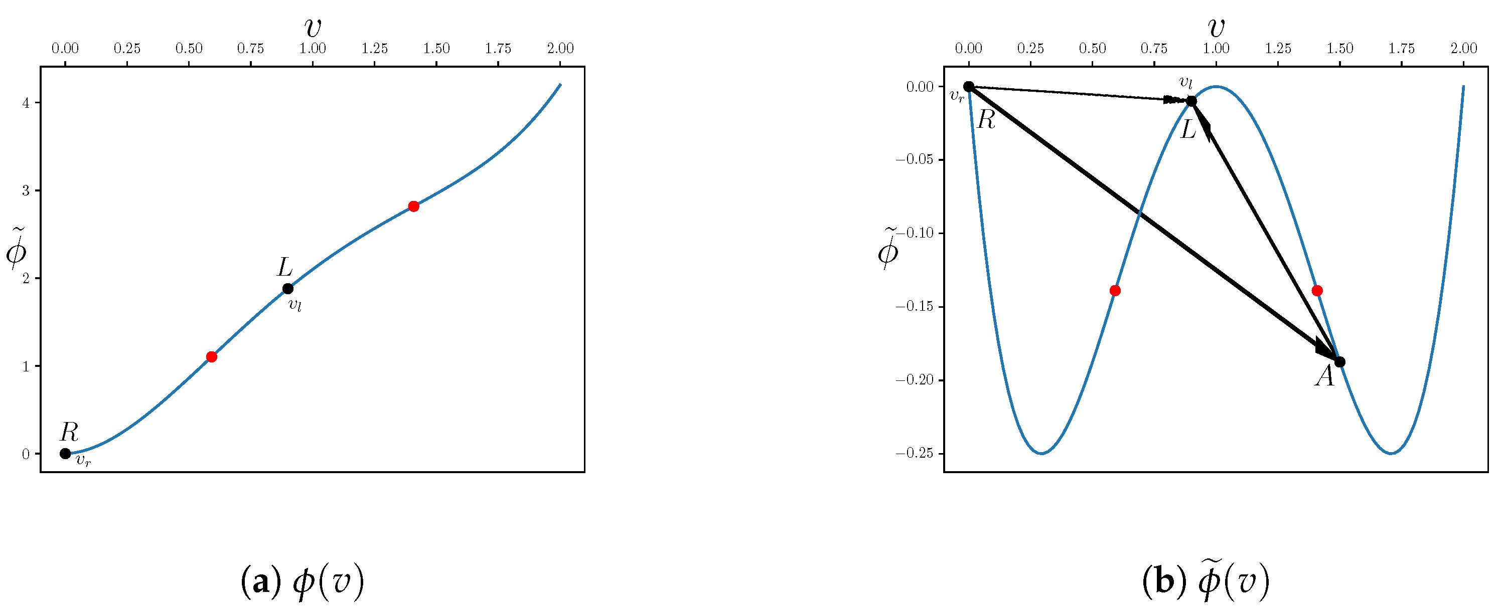
We consider a flow function with two inflection points (Figure 1a):

$$\varphi \left(v\right)={(v-1)}^2\left({(v-1)}^2-1\right)+2.1·v.$$

Using Galilean transformations,

$$x\to \tilde{x}+2.1·t,$$

we can reduce this function to the form (Figure 1b),

$$\tilde{\varphi }\left(v\right)={(v-1)}^2\left({(v-1)}^2-1\right).$$

The graph of the function $\tilde{\varphi }\left(v\right)$ shows more clearly the relative positions of the inflection points, the parameters of the Riemann problem, and the values of the dependent variable behind the undercompressive shock discussed in Section 3. The arrows show the change in the dependent variable in shock waves when solving the Riemann problem.

Now, let us consider different approaches to the numerical solution of the Riemann problem and analyze the dependence of the results on the scheme parameters.

3. Nonconservative Difference Scheme

3.1. Numerical Method

First, we consider a one-parameter family of difference schemes that combine “upwind scheme” and “Standard Leapfrog” schemes.

Let $x_j=j·\Delta x$ ($j=0,\cdots ,N$). We denote $v_j^n=v(x_j,t_n)$. We will further assume that spatial grid step size $\Delta x=(x_N-x_0)/(N+1)$ is fixed. The “upwind” difference scheme (further denoted as R) is

$$R=\left\{\begin{array}{c}\frac{v_j^{n+1}-v_j^n}{\Delta t}+{\varphi }^{\prime }\left(v_j^n\right)\frac{v_j^n-v_{j-1}^n}{\Delta x},{\varphi }^{\prime }\left(v_j^n\right)>0,\hfill \\ \frac{v_j^{n+1}-v_j^n}{\Delta t}+{\varphi }^{\prime }\left(v_j^n\right)\frac{v_{j+1}^n-v_j^n}{\Delta x},{\varphi }^{\prime }\left(v_j^n\right)<0,\hfill \end{array}\right.$$

(7)

where $\Delta t$ is the time step of the scheme.

The upwind method is stable if

$$r=\frac{\Delta t}{\Delta x}<\frac{1}{\underset{j}{max}\left|{\varphi }^{\prime }\left(v_j^n\right)\right|}.$$

(8)

To solve the problem, we use the hybrid scheme constructed using the “Standard Leapfrog” scheme and R

$$(1-\sigma )·R+\sigma ·\left(\frac{v_j^{n+1}-v_j^{n-1}}{2\Delta t}+{\varphi }^{\prime }\left(v_j^n\right)·\frac{v_{j+1}^n-v_{j-1}^n}{2\Delta x}\right)=0,$$

(9)

where $\sigma \in [0,1]$ is a weight coefficient of the “Standard Leapfrog” scheme. The value $\sigma =0$ corresponds to the R scheme, and $\sigma =1$ corresponds to the “Standard Leapfrog” scheme. Consideration of the accuracy and stability of the scheme (9) is contained in the Appendix A. The stability condition (8) holds for this hybrid scheme.

3.2. Calculation Results

Calculations were performed for the rectangular domain

$$x\in [-20,000,20,000],t\in [0,\tilde{t}],\tilde{t}=4000.$$

using various difference-scheme parameters $\sigma$ and r. We analyze the dependency of numerical solutions on these parameters. The values of the parameters used for calculations are

$$\sigma =\{0,0.7,0.8,0.9,0.99\},r=\{0.0125,0.025,0.05,0.1,0.2\}.$$

The numerical algorithm is set out in the Appendix A.

If the parameter r is fixed, the solution depends only on the parameter $\sigma$ for given initial conditions (6). The numerical solution is shown in Figure 2 for $\sigma =0$ and $r=0.025$. This solution with a discontinuity in initial conditions “smears” over several cells after a few time steps and then remains unchanged for $\sigma =0$. The resulting wave has a monotone profile. The dependent variable increases from $v_r=0$ to $v_l=0.9$ in a thin layer. The solution is the shock wave, which is shown in Figure 1b by the arrow $R\to L$.

For $\sigma \in \{0.7,0.8,0.9,0.99\}$ (Figure 3), the decay of the initial discontinuity occurs with the formation of two waves. These shocks are shown in Figure 1b by the arrows $R\to A$ and $A\to L$. The profile of the first wave increases in a thin layer. This corresponds to a shock $R\to A$ with a monotonic structure. In this shock, the dependent variable $v$ changes its value from 0 to $v_A\left(\sigma \right)$, represented by the point A in Figure 3. The value of $v_A$ increases together with $\sigma$ from $1.24$ for $\sigma =0.7$ up to $\approx 1.58$ for $\sigma =0.99$. For $\sigma =0.7,0.8,0.9,0.99$ this shock does not satisfy the Lax condition [13],

$${\varphi }^{\prime }\left(v_A\right)>W.$$

(10)

Note that the Lax condition (10) is satisfied for the profile shown in Figure 2.

The shock wave $A\to L$ propagates behind the leading “smeared” shock (see Figure 3). The dependent variable v decreases from $v_A$ to $v_l=0.9$ in the shock $A\to L$. Unlike the shock $R\to A$, the structure of the shock is non-monotonic $A\to L$, i.e., it corresponds to the focus equilibrium point in the phase space.

The second shock $A\to L$ propagates slower than the leading shock $R\to A$. This leads to an increase in the width of the region of constant solution value $v_A$ between the shocks $A\to L$ and $R\to A$.

The effective width of the structure of both waves tends asymptotically to a fixed value. Starting from a certain number of time steps, this width can be considered constant.

To summarize the above consideration, a sequence of two waves is formed after the initial discontinuity decays. In the first wave, the value of $v(x,t)$ rapidly monotonically increases to a value greater than the left value of the initial profile. In the second wave, the value of $v(x,t)$ decreases non-monotonically to the left value of the initial profile. Each of the waves corresponds to a “smeared” shock. The width of each structure remains constant and depends on the difference-scheme cell size. The second wave lags behind the first, forming a region with a constant value of $v(x,t)$.

Please note that only one “smeared” shock is formed for the case of $\sigma =0$ (Figure 2). The solution $v(x,t)$ monotonically increases from the right value of the initial profile to the left one. Numerical solutions shown in Figure 2 and Figure 3 are obtained using difference schemes of type (9). Although the chosen schemes are stable and approximate the same Equation (1), the solutions differ quantitatively and qualitatively.

Now, we analyze the dependency of the solution $v(x,t)$ on the parameter r for each value of $\sigma$. Calculation results are shown in Figure 4.

The obtained numerical solutions demonstrate the dependence on the value r. The difference between the calculation results is especially noticeable at a moderate value of $\sigma$ (see Figure 4a). Moreover, the speed of resulting waves also depends on the value of r.

4. Conservative Difference Scheme

We consider the following one-parameter family of conservative difference schemes

$$\begin{array}{c}(1-\sigma )·\left(\frac{v_j^{n+1}-v_j^n}{\Delta t}+\frac{\varphi \left(v_{j+\frac{1}{2}}^n\right)-\varphi \left(v_{j-\frac{1}{2}}^n\right)}{\Delta x}\right)+\hfill \\ \hspace{1em}\hspace{1em}\hspace{1em}\hspace{1em}\hspace{1em}\hspace{1em}\hspace{1em}\hspace{1em}\hspace{1em}\hspace{1em}\hspace{1em}\hspace{1em}+\sigma ·\left(\frac{v_j^{n+1}-v_j^{n-1}}{2\Delta t}+\frac{\varphi \left(v_{j+1}^n\right)-\varphi \left(v_{j-1}^n\right)}{2\Delta x}\right)=0,\hfill \end{array}$$

(11)

where

$$\varphi \left(v_{j+1/2}^n\right)=\left\{\begin{array}{cc}\varphi \left(v_j^n\right),\hfill & {\varphi }^{\prime }\left(v_j^n\right)>0,\hfill \\ \varphi \left(v_{j+1}^n\right),\hfill & {\varphi }^{\prime }\left(v_j^n\right)<0\hfill \end{array}\right.,$$

$\sigma$ and $(1-\sigma )$ are weights of explicit “Leapfrog” and “upwind scheme” schemes, respectively. The accuracy and stability of the scheme are discussed in the Appendix A. Computation was performed with a similar algorithm as for the nonconservative scheme.

Calculation results for this family of schemes are shown in Figure 5. Parameters r and $\sigma$ take the values given above.

The results demonstrate the same qualitative dependence on r and $\sigma$ as for the nonconservative case. This dependence is further referred to as the parametric instability of the scheme.

The consideration above leads to the conclusion that nonuniqueness is not related to the conservativeness of the difference scheme but rather arises due to the properties of the problem itself.

5. Occurrence of Parametric Instability

Next, we discuss the parametric instability shown in Figure 4. Let us consider the differential approximation of the mixed scheme (9):

$$\begin{array}{c}\frac{\partial v}{\partial t}+\frac{\partial \varphi \left(v\right)}{\partial x}-\frac{1-\sigma }{2}\left(\Delta x-\left|{\varphi }^{\prime }\left(v\right)\right|\Delta t\right)\left|{\varphi }^{\prime }\left(v\right)\right|\frac{{\partial }^{2}v}{\partial x^2}+\hfill \\ \hspace{1em}\hspace{1em}\hspace{1em}\hspace{1em}\hspace{1em}\hspace{1em}\hspace{1em}\hspace{1em}\hspace{1em}\hspace{1em}\hspace{1em}\hspace{1em}\hspace{1em}\hspace{1em}\hspace{1em}\hspace{1em}+\frac{1}{6}\left(\Delta x^2-{\left({\varphi }^{\prime }\left(v\right)\right)}^2\Delta t^2\right){\varphi }^{\prime }\left(v\right)\frac{{\partial }^{3}v}{\partial x^3}=0.\hfill \end{array}$$

(12)

This expression corresponds to the generalized Korteveg-de Vries-Burgers (gKdVB) equation:

$$\frac{\partial v}{\partial t}+\frac{\partial \varphi \left(v\right)}{\partial x}=\mu \frac{{\partial }^{2}v}{\partial x^2}-m\frac{{\partial }^{3}v}{\partial x^3},\mu >0,m>0.$$

(13)

Equation (13) was derived from a class of diffusive-dispersive Euler equations in [23]. This equation was first considered to investigate the structure of shocks for the generalized Hopf equation in Ref. [11] and later considered in Refs. [8,11,19,21,23,24,25,26,27]. The combination of flux function $\varphi \left(v\right)$ with dispersion yields a rich collection of wave solutions. For our paper, the most important solutions from this collection are traveling undercompressive shocks. The simplest example of a nonlinear equation in one spatial variable that has solutions for undercompressed shock waves is the generalized Korteveg-de Vries-Burgers equation with $\varphi \left(v\right)=v^3$ (see [23]).

Coefficients $\mu$ and m describe small-scale dissipation and dispersion, respectively. Comparing Equation (13) with the differential approximation (12) of the Scheme (9) yields the following expressions:

$$\begin{array}{cc}\hfill \mu \left(v\right)& =\frac{(1-\sigma )}{2}·\left(\Delta x-\Delta t\left|{\varphi }^{\prime }\left(v\right)\right|\right)·\left|{\varphi }^{\prime }\left(v\right)\right|=\frac{(1-\sigma )\Delta x}{2}\left(1-r\left|{\varphi }^{\prime }\left(v\right)\right|\right)·\left|{\varphi }^{\prime }\left(v\right)\right|,\hfill \\ \hfill m\left(v\right)& =\frac{1}{6}\left({(\Delta x)}^2-{(\Delta t)}^2{\left({\varphi }^{\prime }\left(v\right)\right)}^2\right)·{\varphi }^{\prime }\left(v\right)=\frac{{(\Delta x)}^2}{6}(1-r^2{\left({\varphi }^{\prime }\left(v\right)\right)}^2)·{\varphi }^{\prime }\left(v\right),\hfill \end{array}$$

(14)

We consider the problem of the traveling-wave propagation for the gKdVB (13):

$$\begin{array}{c}v=v\left(\xi \right),\xi =x-Wt,\\ \frac{d^{2}v}{d{\xi }^2}-\frac{1}{\gamma }\frac{dv}{d\xi }=Wv-\varphi \left(v\right),\\ \underset{\xi \to +\infty }{lim}v\left(\xi \right)=v_r\equiv 0,\end{array}$$

(15)

where W is the speed of the traveling wave. The solution of this problem depends only on the effective dissipation coefficient $\gamma =\sqrt{m}/\mu$. The value $v\left(\xi \right)$ for $\xi \to -\infty$ satisfies the Hugoniot relation (4).

Equation (14) give the expression for $\gamma$:

$$\gamma =\frac{1}{(1-\sigma )}\sqrt{\frac{2}{3}\frac{(1+\left|{\varphi }^{\prime }\left(v\right)\right|·r)}{(1-\left|{\varphi }^{\prime }\left(v\right)\right|·r){\varphi }^{\prime }\left(v\right)}}.$$

(16)

From (16), it follows that $\gamma$ does not depend on $\Delta t$ and $\Delta x$ for a fixed $r=\Delta t/\Delta x$ and inversely proportional to the weight coefficient $1-\sigma$. Any variation of r and $\sigma$ leads to a change in $\gamma$ and, therefore, changes the numerical solution of the Riemann Problem (5).

For gKdVB (13), it was shown earlier [19,22] that if the decay of an initial discontinuity occurs with the formation of two (or more) waves, then the leading wave always corresponds to a non-classical (special) shock. Non-classical shocks do not satisfy the Lax condition, i.e.,

$$W>{\varphi }^{\prime }\left(v_l\right).$$

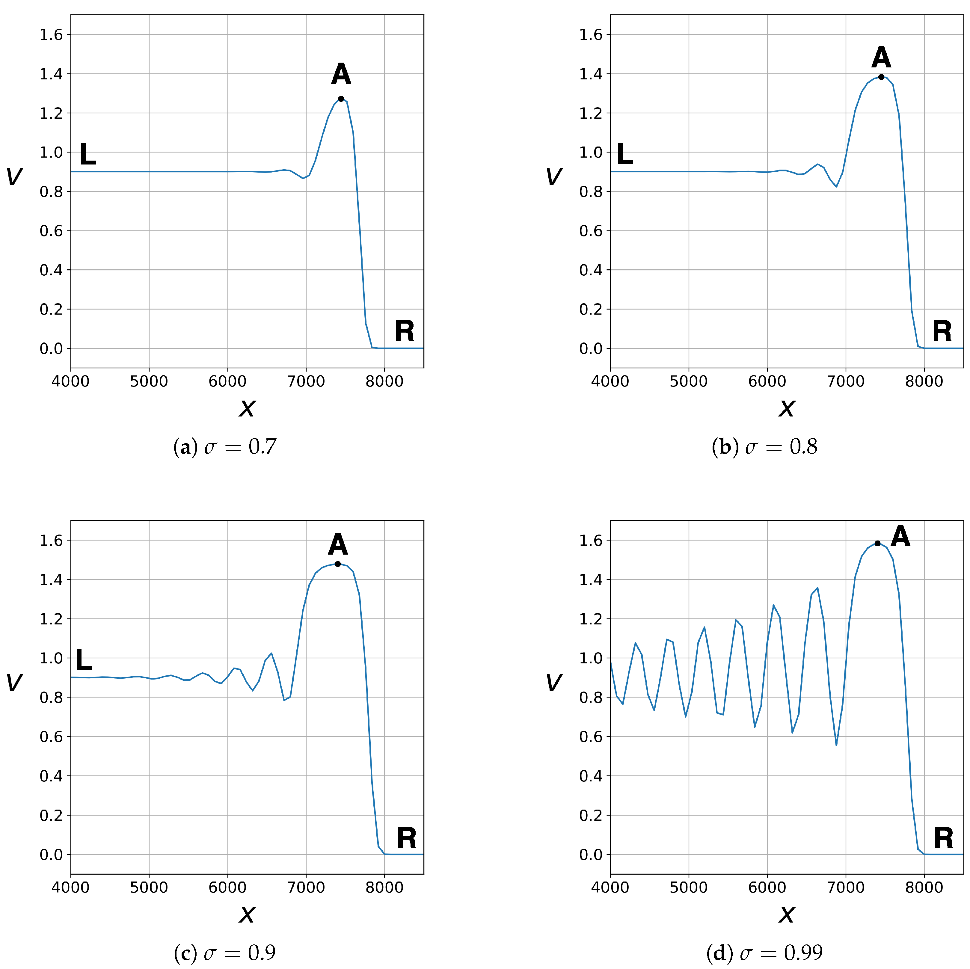
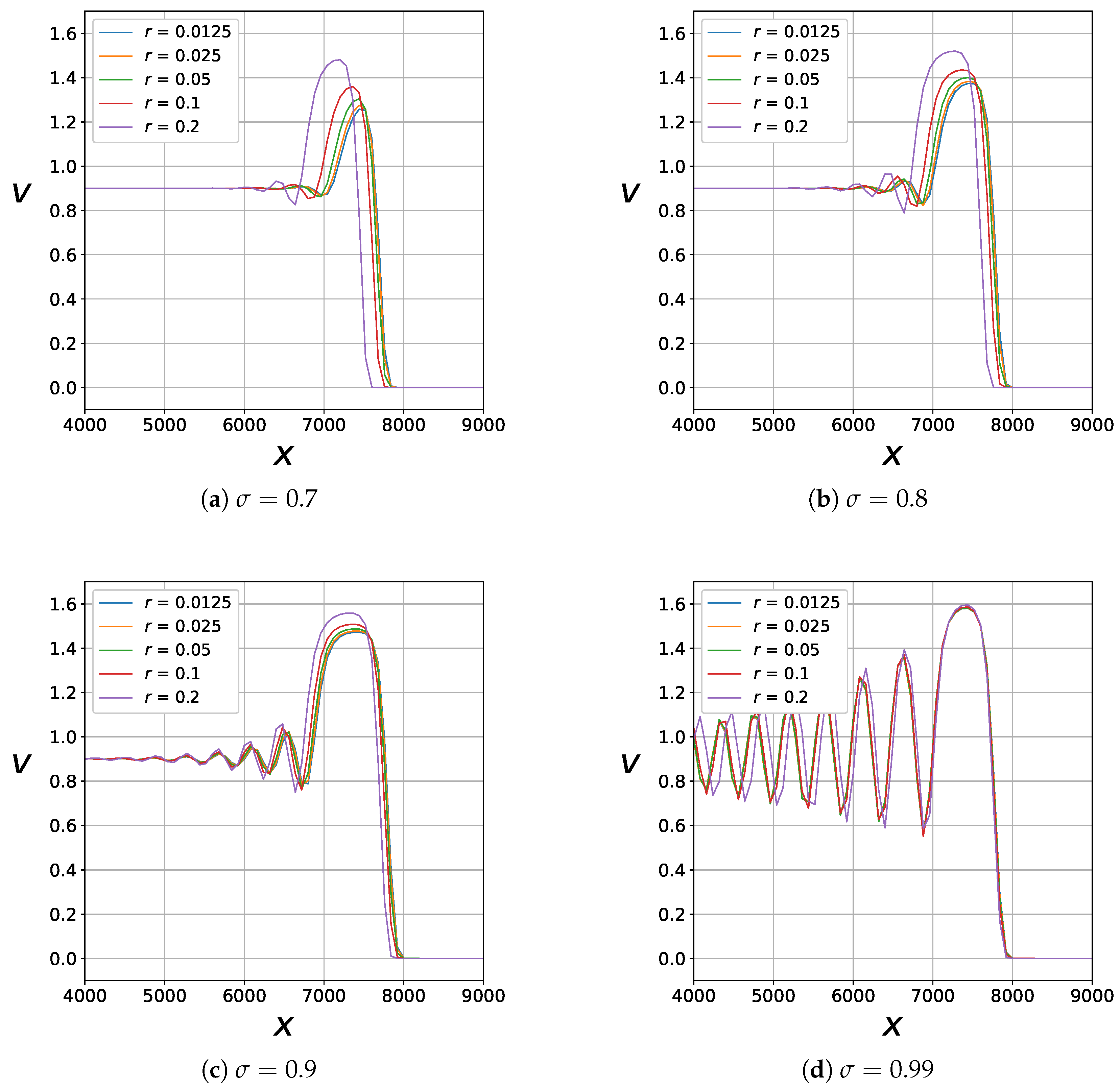
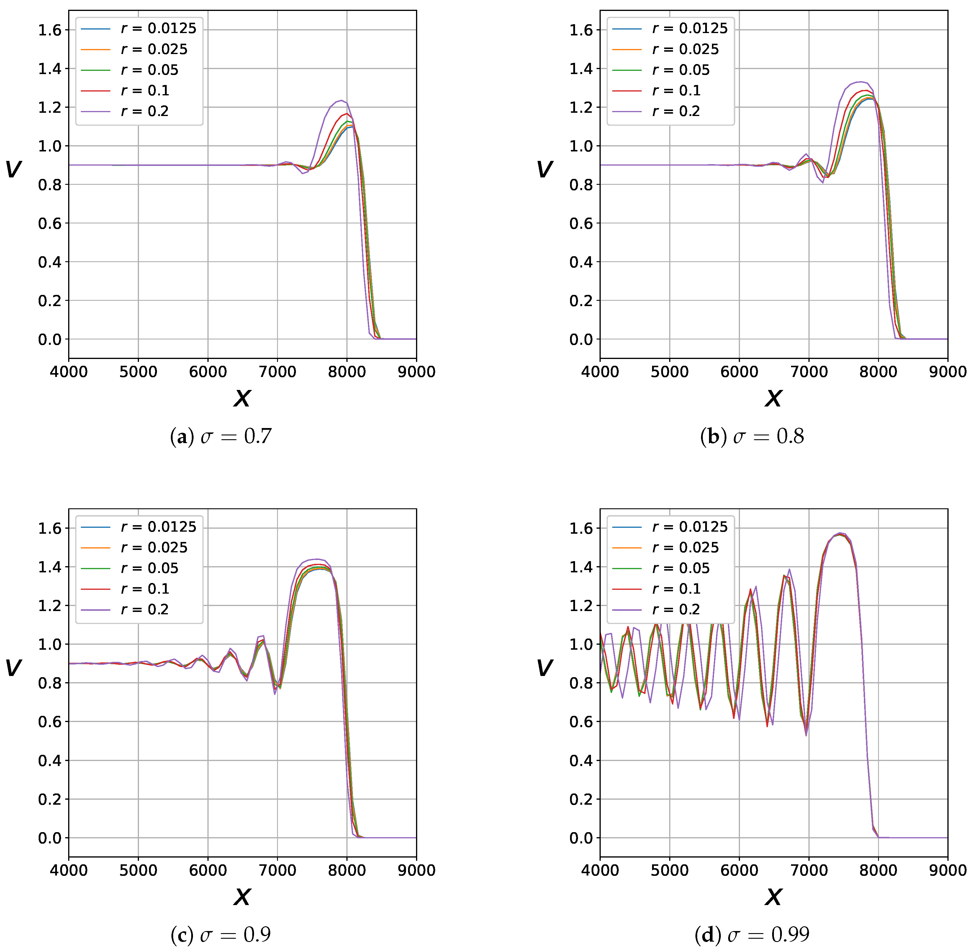
For this reason, a Riemann wave or a classic shock lags behind such an undercompressive shock. Therefore, the width of the intermediate region increases over time. This type of solution is shown in Figure 3.

For classical shocks, the Lax condition is satisfied, i.e.,

$$W<{\varphi }^{\prime }\left(v_l\right).$$

It means that any perturbation reaches such shock in a finite time interval. Hence, there is no solution to the Riemann problem in the form of two subsequent classical shocks.

The occurrence of an undercompressive shock is associated with the existence of inflection points of the flow function $\varphi \left(v\right)$. The speed of the undercompressive shock W is defined by the effective dissipation coefficient $\gamma$. The dissipative and dispersive properties of the given difference scheme determine the latter. For the given family of difference schemes (9), the dissipative effect is determined, in particular, by the value of $1-\sigma$. This effect weakens with the increase of $\sigma$. On the other hand, the scheme dispersion weakens with increasing r.

Let us summarize the results of this section and give a direct answer to the question posed in the title. The numerical solution of the Riemann problem for the generalized Hopf Equation (1) with the flow function having multiple inflection points depends on the particular form of the difference scheme and its parameters. In this case, the exact solution to the Riemann problem is not unique, and the numerical solution converges to one of an infinite set of exact solutions. If value $r=\Delta t/\Delta x$ is not fixed when decreasing the size of the cell $\Delta x$, then the numerical solution can “switch” from one exact solution to another. Since coefficients $\mu$ and m in the corresponding terms of differential approximation depend on the particular choice of the scheme, numerical solutions will converge to different exact solutions for different schemes. Dissipative and dispersive properties of the differential approximation of the difference scheme determine the choice of the exact solution to which the numerical solution converges. The exact solutions of gKdVB are (i) a classical shock (with the Lax condition satisfied), (ii) a non-classical shock, or (iii) a sequence of a non-classical shock, a classical shock, and a Riemann wave. Depending on the properties of the $\varphi \left(v\right)$, there can be several undercompressive shocks, but only one of them is stable (see Ref. [19] for further details). The speed of the stable undercompressive shock depends on $\mu$ and m, and this shock is the leading wave in Figure 2, Figure 3, Figure 4 and Figure 5.

In the case of the convex flow function, there are no undercompressive shocks. If the chosen difference scheme is stable and “smears” discontinuities, then numerical solutions of the generalized Hopf equation converge to the same one.

Please note that the numerical solutions converge to the same solution for any difference scheme with strong dissipation (small $\gamma$).

In the next section, we discuss how to use this information to regularize the difference method.

6. Recipe for a Proper Difference Scheme

The problem of the parametric instability of the difference scheme cannot be definitely solved in the frame of the generalized Hopf equation. It means that it is impossible to specify the only correct numerical solution of the Riemann problem without detailed information on the real physical dissipative and dispersive properties of the medium in a thin shock layer, namely coefficients ${\mu }_{real}$ and $m_{real}$.

The dissipative and dispersive effects of the scheme itself can be suppressed by artificial dissipation and dispersion. Let us consider the gKdVB equation with some “effective” dissipation and dispersion coefficients:

$$\frac{\partial v}{\partial t}+\frac{\partial \varphi \left(v\right)}{\partial x}={\mu }_0\frac{{\partial }^{2}v}{\partial x^2}-m_0\frac{{\partial }^{3}v}{\partial x^3}.$$

(17)

Suppose that ${\mu }_0$ and $m_0$ are constant and positive.

The construction of a difference scheme for this equation is reduced to using one of the schemes presented above for the left side of the equation and choosing the appropriate difference approximations for the higher-order derivatives. We can write the P-form for the right-hand side Approximation (12) without detailing a specific choice of such approximations. The P-form gives

$$\frac{\partial v}{\partial t}+\frac{\partial \varphi \left(v\right)}{\partial x}-\left({\mu }_0+\mu \right)\frac{{\partial }^{2}v}{\partial x^2}+\left(m+m_0\right)\frac{{\partial }^{3}v}{\partial x^3}\approx 0.$$

(18)

Expressions for $\mu$ and m are given in (14).

The specific choice of the difference approximation for this equation’s dissipative term can lead to additional dispersive terms appearing in (17). For the sake of simplicity, suppose that such approximation does not modify the total dispersion coefficient $m_0+m$.

The existence of artificial dissipation and dispersion can suppress the corresponding effects of the difference scheme if ${\mu }_0$ and $m_0$ satisfy the condition:

$${\mu }_0\gg \mu ,m_0\gg m.$$

Additionally, we should include the condition of numerical stability (8). We can analyze expressions for coefficients (14) to obtain desired values of ${\mu }_0$ and $m_0$.

The condition (8) guarantees that

$$r|{\varphi }^{\prime }\left(v\right)|<1.$$

Using this fact, we obtain the inequalities

$$\mu <\frac{(1-\sigma )\Delta x}{2}\left|{\varphi }^{\prime }\left(v\right)\right|,m<\frac{{(\Delta x)}^2}{6}{\varphi }^{\prime }\left(v\right).$$

Now we denote

$$M=sup|{\varphi }^{\prime }\left(v\right)|,$$

where the supremum is taken on the interval of $v$ that includes inflection points of the flow function.

Thus, we obtain the desired suppression conditions:

$${\mu }_0\gg \frac{(1-\sigma )\Delta x}{2}M,m_0\gg \frac{{(\Delta x)}^2}{6}M.$$

(19)

The choice of coefficients ${\mu }_0$, $m_0$ could not be made independently if real (physical) dissipation and dispersion coefficients of the medium ${\mu }_{real}$ and $m_{real}$ are known. Let us now consider the following property of the Riemann problem for Equation (17): the exact solution is defined by the value $\gamma =\sqrt{m}/\mu$. Therefore, we can choose ${\mu }_0$, $m_0$ so that the relation holds

$${\gamma }_0=\frac{\sqrt{m_0}}{{\mu }_0}=\frac{\sqrt{m_{real}}}{{\mu }_{real}}.$$

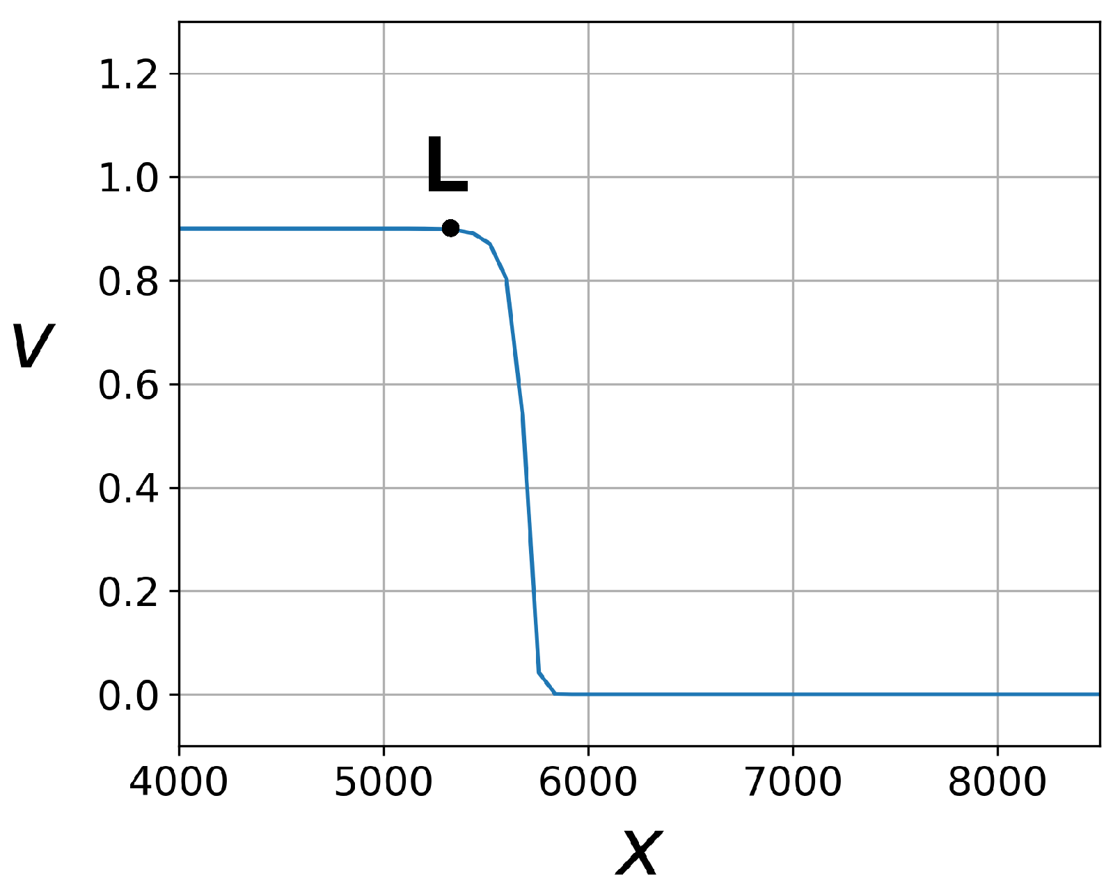
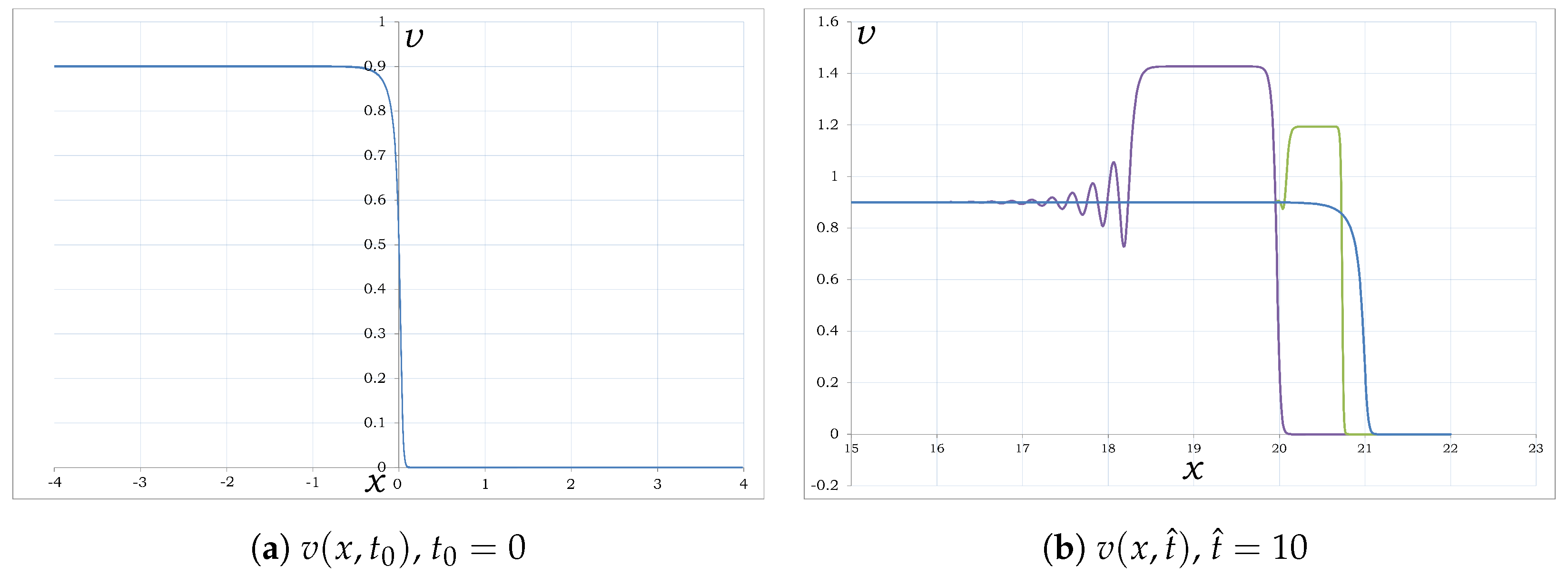
Let us set the initial condition as a smeared step:

$$v(x,0)=\left\{\begin{array}{c}{v}_l,x<0,\hfill \\ v_l-140·(v_r-v_l)\left(\frac{1}{7}{\left(\frac{x}{b}\right)}^7-\frac{1}{2}{\left(\frac{x}{b}\right)}^6+\frac{3}{5}{\left(\frac{x}{b}\right)}^5-\frac{1}{4}{\left(\frac{x}{b}\right)}^4\right),\hfill \\ v_r,x>0.\hfill \end{array}\right.$$

(20)

The function $v(x,0)$ with $v_r=0$, $v_l=0.9$ and $b=0.1$ is shown in Figure 6a. Numerical solutions of the Cauchy Problem (17) and (20) do not depend on the difference schemes because the solution of the problem is unique. The numerical solutions are uniquely defined by the parameters $\mu$ and m. Representations of the Cauchy problem solutions for the gKdVB Equation (17) with $v_r=0$, $v_l=0.9$ and $b=0.1$ are shown in Figure 6b. The left-hand side of Equation (17) is approximated by the “Leapfrog” scheme ($\sigma =0$).

Finally, assume there is no physical model of the medium, so the parameters ${\mu }_{real}$ and $m_{real}$ are unknown. In this case, we can estimate the upper and lower bounds of the Riemann problem solution $v(x,t)$. This requires calculations for sufficiently large and small values of ${\gamma }_0$. This approach gives correct results for the cases of strong dissipation/weak dispersion (${\gamma }_0\ll 1$) and weak dissipation/strong dispersion (${\gamma }_0\gg 1$).

7. Conclusions

We have considered various approaches to the numerical solution of the generalized Hopf equation with a flow function having two inflection points to answer the question in the title. Stable finite-difference schemes can converge to different solutions for the generalized Hopf equation because the solution of the Riemann problem is not unique. In this case, the numerical solution of the Riemann problem is not unique too, and we show the dependence of the result on the parameters of the nonconservative and conservative difference schemes. Numerical solutions can converge to different exact solutions. This result depends on the weighting factor $\sigma$ and the grid parameter $r=\Delta t/\Delta x$ not only quantitatively but also qualitatively. This difference is explained by the dissipative and dispersive effects due to the properties of the difference scheme.

Considering the peculiarities of the generalized Korteveg-de Vries-Burgers equation with a flow function having multiple inflection points allows us to formulate an approach to construct a “stable” difference scheme.

Within this approach, the correct choice of solution to the Riemann problem is based on the physical properties of the medium.

Calculation using real (physical) dissipation and dispersion coefficients ${\mu }_{real},m_{real}$ seems to be irrational because it requires multiscale calculation. Such a calculation is usually expansive (or impossible). Instead, we propose to use artificial dissipation and dispersion such that

1.

the artificial coefficients ${\mu }_0$ and $m_0$ are big enough, so the similar effects due to the difference scheme are suppressed,

2.

the coefficients should be chosen to hold the ratio $\sqrt{m_0}/{\mu }_0=\sqrt{m_{real}}/{\mu }_{real}$, which gives a correct numerical solution of the Riemann problem.

References

1. Kulikovskii, A.G.; Pogorelov, N.V.; Semenov, A.Y. Mathematical Aspects of Numerical Solution of Hyperbolic Systems. In Proceedings of the Hyperbolic Problems: Theory, Numerics, Applications; Jeltsch, R., Fey, M., Eds.; Birkhäuser: Basel, Switzerland; Boston, MA, USA; Berlin, Germany, 1999; pp. 589–598. [Google Scholar]
2. Likhachev, A.P. Mechanism of the appearance of the cellular structure of a shock wave in the region of its ambiguous representation. High Temp. 2012, 50, 506–511. [Google Scholar] [CrossRef]
3. Lomonosov, I. Multi-phase equation of state for aluminum. Laser Part. Beams 2007, 25, 567–584. [Google Scholar] [CrossRef]
4. Lomonosov, I.; Tahir, N. Theoretical investigation of shock wave stability in metals. Appl. Phys. Lett. 2008, 92, 101905. [Google Scholar] [CrossRef]
5. Gel’fand, I. Some problems in the theory of quasilinear equations. Usp. Mat. Nauk. 1959, 14, 87–158. [Google Scholar]
6. Oleinik, O.A. Uniqueness and stability of the generalized solution of the Cauchy problem for a quasi-linear equation. Uspekhi Mat. Nauk. 1959, 14, 165–170. [Google Scholar]
7. Goritskii, A.Y.; Kruzhkov, S.N.; Chechkin, G.A. First Order Partial. Differ. Equations; Department of Mechanics and Mathematics, MSU: Moscow, Russia, 1999. [Google Scholar]
8. Hayes, B.; Shearer, M. Undercompressive Shocks and Riemann Problems for Scalar Conservation Laws with Nonconvex Fluxes. R. Soc. Edinb.-Proc. 1999, 129, 733–754. [Google Scholar] [CrossRef]
9. Bedjaoui, N.; LeFloch, P.G. Diffusive–Dispersive Traveling Waves and Kinetic Relations: Part I: Nonconvex Hyperbolic Conservation Laws. J. Differ. Equ. 2002, 178, 574–607. [Google Scholar] [CrossRef]
10. Bedjaoui, N.; LeFloch, P.G. Diffusive–Dispersive travelling waves and kinetic relations V. Singular diffusion and nonlinear dispersion. Proc. R. Soc. Edinb. Sect. Math. 2004, 134, 815–843. [Google Scholar] [CrossRef]
11. Kulikovskii, A.G. The possible effect of oscillations in a discontinuity structure on the set of admissible discontinuities. Dokl. Akad. Nauk. SSSR 1984, 275, 1349–1352. [Google Scholar]
12. Kulikovskii, A.G. Strong discontinuities in flows of continua and their structure. Proc. Steklov Inst. Math. 1990, 182, 285–317. [Google Scholar]
13. Lax, P.D. Hyperbolic systems of conservation laws. Commun. Pure Appl. Math. 1957, 10, 537–566. [Google Scholar] [CrossRef]
14. Hayes, B.T.; Shearer, M. A nonconvex scalar conservation law with a trilinear flux. Q. Appl. Math. 2001, 59, 615–635. [Google Scholar] [CrossRef]
15. Samokhin, A. Reflection and Refraction of Solitons by the KdV–Burgers Equation in Nonhomogeneous Dissipative Media. Theor. Math. Phys. 2018, 197, 1527–1533. [Google Scholar] [CrossRef]
16. Samokhin, A. The KdV soliton crosses a dissipative and dispersive border. Differ. Geom. Its Appl. 2021, 75, 101723. [Google Scholar] [CrossRef]
17. Chugainova, A.P.; Shargatov, V.A. Traveling waves and undercompressive shocks in solutions of the generalized Korteweg–de Vries–Burgers equation with a time-dependent dissipation coefficient distribution. Eur. Phys. J. Plus 2020, 135, 1–18. [Google Scholar] [CrossRef]
18. Shargatov, V.A.; Chugainova, A.P. Stability analysis of traveling wave solutions of a generalized Korteweg–de Vries–Burgers equation with variable dissipation parameter. J. Comput. Appl. Math. 2021, 397, 113654. [Google Scholar] [CrossRef]
19. Shargatov, V.A.; Chugainova, A.P.; Tomasheva, A.M. Structures of Classical and Special Discontinuities for the Generalized Korteweg–de Vries–Burgers Equation in the Case of a Flux Function with Four Inflection Points. Proc. Steklov Inst. Math. 2023, 322, 257–272. [Google Scholar] [CrossRef]
20. Lyapidevskii, V.Y.; Teshukov, V. Mathematical Models of Propagation of Long Waves in an Inhomogeneous Fluid; Publishing House of the Siberian Branch of the Russian Academy of Sciences: Novosibirsk, Russia, 2000. [Google Scholar]
21. Pego, R.L.; Smereka, P.; Weinstein, M.I. Oscillatory instability of traveling waves for a KdV-Burgers equation. Phys. Nonlinear Phenom. 1993, 67, 45–65. [Google Scholar] [CrossRef]
22. Chugainova, A.P.; Shargatov, V.A. Analytical description of the structure of special discontinuities described by a generalized KdV-Burgers equation. Commun. Nonlinear Sci. Numer. Simul. 2019, 66, 129–146. [Google Scholar] [CrossRef]
23. El, G.A.; Hoefer, M.A.; Shearer, M. Dispersive and Diffusive-Dispersive Shock Waves for Nonconvex Conservation Laws. Siam Rev. 2017, 59, 3–61. [Google Scholar] [CrossRef]
24. Kulikovskii, A.G.; Sveshnikova, E.I. On the decay of an arbitrary initial discontinuity in an elastic medium. Prikl. Mat. Mekh. 1988, 52, 1007–1012. [Google Scholar] [CrossRef]
25. Pego, R.L.; Weinstein, M.I. Eigenvalues, and instabilities of solitary waves. Philos. Trans. R. Soc. London. Ser. Phys. Eng. Sci. 1992, 340, 47–94. [Google Scholar] [CrossRef]
26. Shearer, M.; Schecter, S. Undercompressive shocks for nonstrictly hyperbolic conservation laws. J. Dyn. Differ. Equ. 1990, 3, 199–271. [Google Scholar]
27. LeFloch, P.D.; Shearer, M. Non-classical Riemann solvers with nucleation. Proc. R. Soc. Edinb. Sect. Math. 2004, 134, 961–984. [Google Scholar] [CrossRef]
28. Isaacson, E.; Keller, H. Analysis of Numerical Methods; Dover Books on Mathematics, Dover Publications: Garden City, NY, USA, 1994. [Google Scholar]
29. Lax, P.D.; Richtmyer, R.D. Survey of the stability of linear finite difference equations. Commun. Pure Appl. Math. 1956, 9, 267–293. [Google Scholar] [CrossRef]
Figure 1. Plot of the flow function in different coordinate systems with the inflection points marked (red); v l and v r — the parameters of the Riemann Problem (5).
Computation 12 00076 g001
Figure 2. Solution v ( x , t ˜ ) obtained by the R Scheme; t ˜ = 4000 , σ = 0 , r = 0.025 .
Computation 12 00076 g002
Figure 3. Numerical solution v ( x , t ˜ ) for r = 0.025 and various σ obtained using the nonconservative difference scheme; t ˜ = 4000 , r = 0.025 .
Computation 12 00076 g003
Figure 4. Numerical solution v ( x , t ˜ ) for various r and σ obtained using the nonconservative difference scheme; t ˜ = 4000 .
Computation 12 00076 g004
Figure 5. Numerical solution v ( x , t ˜ ) for various r and σ obtained using the conservative difference scheme; t ˜ = 4000 .
Computation 12 00076 g005
Figure 6. The gKdVB Cauchy problem solutions with diffusive-dispersive shock waves: (a) initial distribution; (b) numerical solutions of the Cauchy problem for gKdVB with the same step-like initial conditions with μ = 0.03535 , m = 0.000065 (blue), μ = 0.003535 , m = 0.000065 (green) and μ = 0.003535 , m = 0.00065 (purple).
Computation 12 00076 g006
Disclaimer/Publisher’s Note: The statements, opinions and data contained in all publications are solely those of the individual author(s) and contributor(s) and not of MDPI and/or the editor(s). MDPI and/or the editor(s) disclaim responsibility for any injury to people or property resulting from any ideas, methods, instructions or products referred to in the content.