Overlapping Grid-Based Spectral Collocation Technique for Bioconvective Flow of MHD Williamson Nanofluid over a Radiative Circular Cylindrical Body with Activation Energy

Abstract

The amalgamation of motile microbes in nanofluid (NF) is important in upsurging the thermal conductivity of various systems, including micro-fluid devices, chip-shaped micro-devices, and enzyme biosensors. The current scrutiny focuses on the bioconvective flow of magneto-Williamson NFs containing motile microbes through a horizontal circular cylinder placed in a porous medium with nonlinear mixed convection and thermal radiation, heat sink/source, variable fluid properties, activation energy with chemical and microbial reactions, and Brownian motion for both nanoparticles and microbes. The flow analysis has also been considered subject to velocity slips, suction/injection, and heat convective and zero mass flux constraints at the boundary. The governing equations have been converted to a non-dimensional form using similarity variables, and the overlapping grid-based spectral collocation technique has been executed to procure solutions numerically. The graphical interpretation of various pertinent variables in the flow profiles and physical quantities of engineering attentiveness is provided and discussed. The results reveal that NF flow is accelerated by nonlinear thermal convection, velocity slip, magnetic fields, and variable viscosity parameters but decelerated by the Williamson fluid and suction parameters. The inclusion of nonlinear thermal radiation and variable thermal conductivity helps to enhance the fluid temperature and heat transfer rate. The concentration of both nanoparticles and motile microbes is promoted by the incorporation of activation energy in the flow system. The contribution of microbial Brownian motion along with microbial reactions on flow quantities justifies the importance of these features in the dynamics of motile microbes.

1. Introduction

Investigation of non-Newtonian fluidic models is a subject of curiosity for many researchers because of their nature, engineering, and industrial solicitations, including polymeric melt, crystal growing, dilute polymer solutions, drilling muds, cosmetic products, foods, coated sheets, and glass blowing. From a previous analysis, it is clear that many constitutional correlations have been put forward to flaunt the knotty traits of non-Newtonian fluids. Such entrenchment emerges from the view that the indispensable features of non-Newtonian liquids cannot be scrutinized using the classical Navier–Stokes equations, which are solely applicable to determine Newtonian fluid traits. Numerous researchers have investigated the behaviour of non-Newtonian fluids through various geometrical configurations. Among these geometries we have cylindrical surfaces, which play a significant role in polymer processing systems. Nazar et al. [1] investigated mixed convective flow of micropolar fluids through a horizontal circular cylinder for the case of constant surface temperature. Madhavi et al. [2,3,4] and Gaffar et al. [5] scrutinized third-grade fluid flow through a horizontal cylinder surface. Gaffar et al. [6] also explored boundary layer flow and the heat relocation of tangent hyperbolic fluid across a horizontal circular cylindrical body with first-order thermal and velocity slip. Nagaraj et al. [7] investigated flow and heat relocation in non-Newtonian Eyring–Powell fluids over a horizontal circular cylindrical surface by taking into account suction/blowing and heat convective boundary constraints. Zokri et al. [8] studied the flow of non-Newtonian Jeffrey fluids over a horizontal circular cylinder in the company of mixed convection and viscous heating effects.

The non-Newtonian fluid model for Williamson fluids was introduced by Williamson [9], and it has been confirmed to be among the predominantly crucial non-Newtonian fluids due to its low viscosity and higher shear rate. In particular, the Williamson fluid model predicts that the effective viscosity will decline monotonically with an elevation in the shear rate and vice versa. This pseudo-plastic fluid deportment is one instance of the various ways in which this non-Newtonian liquid might be usable in modern technology and industry. The applicability of Williamson fluid in technologies and industries has generated a major effect on manufacturing processes. Thus, many scholars have been involved in the exploration of features of Williamson fluids in the improvement of the thermal features of this fluid. However, just like any other non-Newtonian fluid, the Williamson fluid is still incapable of fulfilling the demand for superior extremity heat transport due to its dissatisfying thermal conductivity. To upsurge thermal conductivity as well as enhance heat transport performance, the theory of adding nanoparticles (NPs) into the non-Newtonian fluid has proven to be one of the more contemporaneously innovative concepts in the recent past years. The mixture of NPs and the host fluid is called a nanofluid (NF) [10]. Various models have been put forward to scrutinize NFs, of which the Buongiorno NF model [11] is one of them. The Buongiorno [11] NF model is a two-phase model that focuses on Brownian motion and thermophoresis impacts, and this model plays a significant role when the movement of NPs remarkably impacts the fluid flow. Another notable model is the Tiwari–Das NF model [12], which is a single-phase model that is concerned with studying the volume fraction of NPs. Rashad et al. [13] used the Buongiorno NF model to analyze the combined convection flow of a Newtonian NF across a horizontal circular cylinder immersed in a penetrable medium with heat-convective boundary conditions. Using the Tiwari–Das NF model, Zokri [14] also studied the mixed convection flow of Jeffrey NFs past a horizontal cylinder by accounting for suction/injection and heat convective boundary constraints. Merkin [15] initiated the study of fluid flow moving through a horizontal circular cylinder with mixed convection, and many studies were reported thereafter. Mixed convection plays a major role in enhancing the thermal features of heat transport. It also accounts for the general instance of convection that takes place in various industrial and technological solicitations including electronic device cooling, solar energy storage, drying technology, food processing, and float glass manufacturing.

In many engineering, technological, and industrial processes, the disparity between the surface and ambient (free stream) temperatures need not be small. In the instance of huge temperature variations, the fluid and heat transfer features are remarkably influenced. In such instances, accounting for linear Boussinesq approximation and classical linear Rosseland approximation in the fluid and heat transport equations, respectively, is inadequate, and that can lead to a reduction in the quality of the results. Consequently, it is mandatory to account for nonlinear Boussinesq approximations and nonlinear Rosseland thermal radiation in such instances so that accurate results are achieved. Practical examples of nonlinear thermal convection include engineering, geophysical, and astrophysical flows. On the other hand, nonlinear Rosseland heat radiation plays a fundamental role in manufacturing processes with larger temperature differences. EL-Zahar et al. [16] employed the modified Tiwari–Das NF to investigate the magnetized mixed convective flow of hybrid NFs across a horizontal circular cylindrical surface by considering nonlinear thermal radiation. Basha et al. [17] used the Buongiorno NF model to analyze the mixed convection flow of tangent hyperbolic NFs through a horizontal circular cylinder by accounting for nonlinear Boussinesq estimation. Activation energy (AE) is the minimal quantity of energy needed by chemical reactants to go through a chemical reaction. Mass transport procedures together with chemical reactions with Arrhenius AE emerge in areas of chemical engineering and food processing. Huang [18] studied free convective flow via a horizontal circular cylindrical surface immersed in a penetrable medium with AE and suction/injection.

Bioconvection is a phenomenon whereby the flow and thermal features of the fluid are impacted by the existence of microbes. Bioconvection flows emerge in various fascinating solicitations in environmental systems, fuel cells, and biological polymer synthesis [19]. The upward swimming microorganisms give rise to unstable density stratification, and because of that, bioconvection takes place in the fluid. In other words, bioconvection is compelled by instability that emerges due to self-propelled microorganisms swimming to and interacting with NPs and buoyancy [20,21,22,23]. The amalgamation of bioconvection and NF has yielded some exceptional results in micro-fluidic devices such as micro-channels and micro-rectors. Kuznestov and Avramenko [24] initiated the use of NPs to scrutinize the bioconvection of gyrotactic microorganisms. Hill and Pedly [25] provided a review study of the hydrodynamics of bioconvection. Through the use of Navier–Stokes equations, Allouit et al. [26] investigated the bioconvection of gyrotactic microorganisms via a vertical cylinder. Mallikarjuna [27] scrutinized the mixed bioconvective flow of a NF containing gyrotatic microorganisms from a vertical slender cylindrical surface. Rashad et al. [28] investigated mixed the bioconvective flow of a Newtonian NF comprising gyrotactic microbes through a horizontal circular cylinder in the company of heat-convective and zero mass flux boundary conditions.

The literature review, particularly investigations by Rashad et al. [13,28], reveals that there is no study on the bioconvective flow of non-Newtonian Williamson NFs in thermal and mass relocation mechanisms over a cylindrical surface with the following research gaps that result in the novelties of the present analysis.

• The complex rheology features of Williamson materials are examined using the modified Buongiorno NF model in the presence of an applied magnetic field, porous media, and variable fluid viscosity.
• Nonlinear Boussinesq approximation and nonlinear Rosseland thermal radiation are incorporated in the momentum and energy equations, respectively, to cater for large temperature differences.
• Heat generation/assimilation and variable thermal conductivity are incorporated in the heat equation for the characterization of energy transfer mechanisms.
• The modified Arrhenius AE, chemical and microbial reactions, NP and microbial Brownian diffusions are considered in the NP concentration and motile microorganism equations for characterization of mass and motile microbes transfer mechanisms.

The main objective of the current analysis is to scrutinize the bioconvective flow, heat, mass, and motile microbes transfer features of the magnetized Williamson NF model containing motile gyrotactic microbes through a horizontal circular cylindrical surface encased in a porous medium. The consequences of nonlinear thermal convection, nonlinear heat radiation, heat generation/assimilation, varying fluid attributes, AE with chemical and microbial reactions, and Brownian motion for both NPs and motile microbes are further elaborated as novelties. There has been limited research conducted on the influence of microbial Brownian motion in conjunction with microbial reactions on fluid flow properties [29,30]. Moreover, the entire flow analysis has been subjected to first-order velocity slips, suction/injection, and heat-convective and zero mass flux constraints at the boundary. The consideration of mixed convective flow of non-Newtonian NF through a heated horizontal cylinder plays a fundamental role in geological, technological, and industrial processes including the thermal recuperation of oil, geothermal reservoirs, insulating wires, drag reduction, thrust bearing, assessment of aquifers, and underground nuclear waste storage. An efficient and accurate overlapping grid-based multi-domain bivariate spectral local linearization method (OMD-BSLLM) [31,32,33] is executed to procure approximate solutions to the complex fluid flow model. The impact of various pertinent variables on the flow profiles and physical quantities of engineering attentiveness is scrutinized through graphical representations.

2. Mathematical Modeling

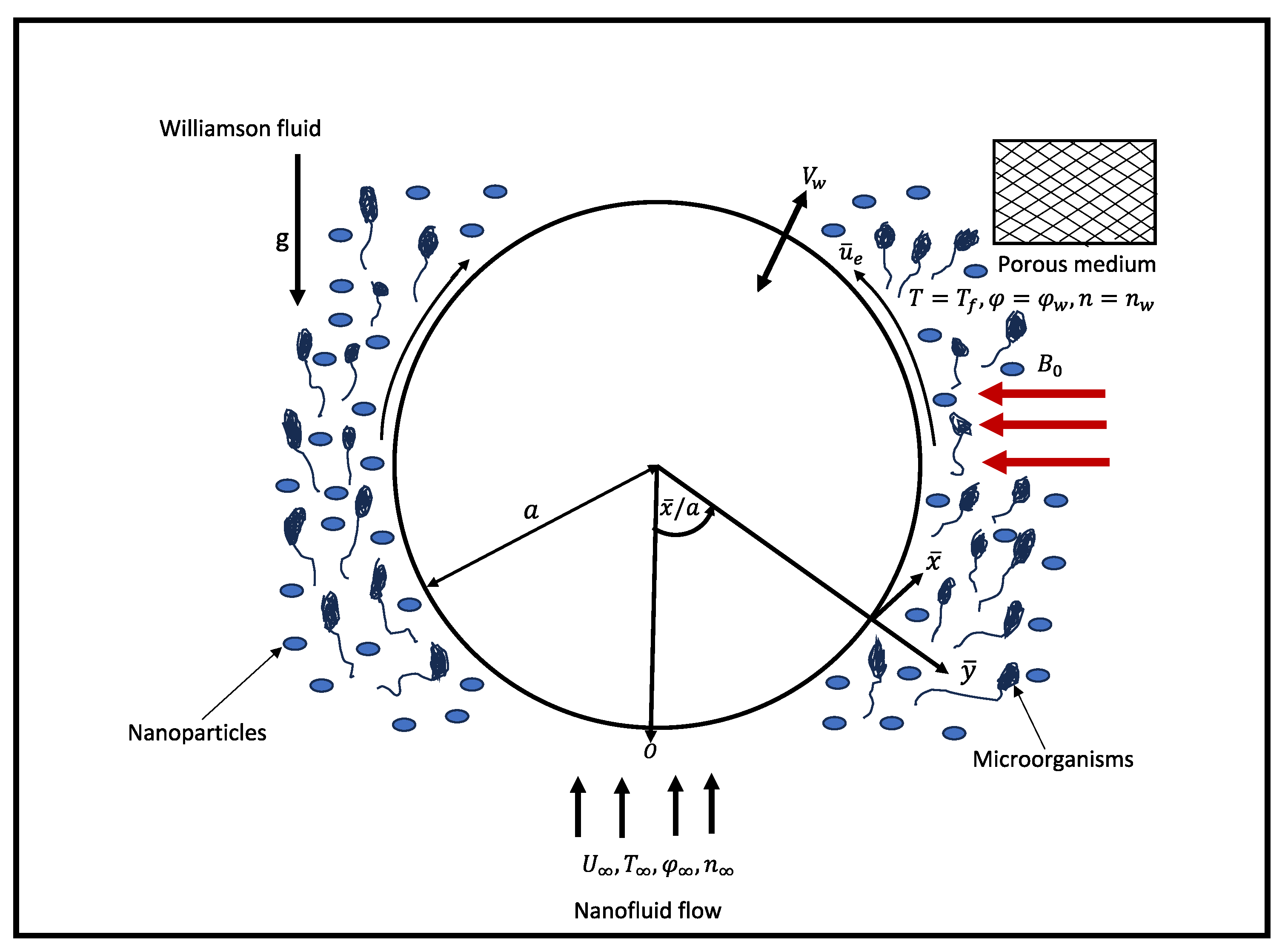
We contemplate the two-dimensional, laminar, steady, incompressible, and viscous nonlinear mixed convective boundary layer flow of Williamson NFs comprising gyrotactic microbes that swim from a horizontal circular cylindrical surface immersed in a porosity medium. The pictorial representation of the flow model and the physical coordinate system is depicted in Figure 1, where a is the radius of the cylinder. The $\overline{x}$ and $\overline{y}$ coordinates are, respectively, measured alongside the surface of the cylinder, resuming from the lower stagnation point, and normal to the cylinder. The uniform magnetic field intensity is enforced parallel to the fluid movement. Fluctuations in density for the buoyant expression are established by utilizing non-linear Boussinesq estimation, and the basic fluid and NPs are in a thermal equilibrium state. The surface of the cylinder is heated via convection from the heated fluid at the temperature $T_f,$ which produces a heat transport coefficient $h_f.$ The cylinder’s surface is maintained at a constant temperature $T_f,$ which is assumed to be greater than the free stream (ambient) temperature $(T_f>T_{\infty })$ for the warmed surface (aiding flow) and lower than the ambient temperature $(T_f<T_{\infty })$ for the cooled surface (reversing flow). The velocity of the external flow is represented by ${\overline{u}}_e\left(\overline{x}\right)=U_{\infty }sin\left(\frac{\overline{x}}{a}\right),$ where $U_{\infty }$ is the ambient velocity. The surface of the cylinder is also maintained at a uniform density of motile microbes $n_w$, whereas the uniform NP volume fraction and density of motile microbes far-off from the cylindrical surface are signified by ${\phi }_{\infty }$ and $n_{\infty },$ respectively. Due to the absence of agglomeration and accumulation of NPs, the NF suspension is dilute (i.e homogeneous dispersion is attained). Furthermore, it is presumed that NPs have no impact on the direction and velocity of the gyrotactic microbes’ swimming. It is worth noting that the velocity for motile microbes, NPs, and the basic fluid is the same. For the characterization of heat transportation, features of nonlinear thermal radiation, heat sink/source, and variable thermal conductivity are involved in the heat (energy) equation. However, for the characterization of mass and motile microbes transportation, features of AE, chemical and microbial reactions, and NP and microbial Brownian motions are invoked in the equations of NP species concentration and motile microbe density conservation. In view of the aforementioned presuppositions, the entire fundamental equations of the flow problem take the form [13,28].

$$\begin{array}{ccc}& & \frac{\partial \overline{u}}{\partial \overline{x}}+\frac{\partial \overline{v}}{\partial \overline{y}}=0,\hfill \\ & & {\rho }_{f\infty }\left(\overline{u}\frac{\partial \overline{u}}{\partial \overline{x}}+\overline{v}\frac{\partial \overline{u}}{\partial \overline{y}}\right)={\rho }_{f\infty }{\overline{u}}_e\frac{d{\overline{u}}_e}{d\overline{x}}+\frac{\partial }{\partial \overline{y}}\left(\mu \left(T\right)\frac{\partial \overline{u}}{\partial \overline{y}}\right)+\sqrt{2}\mathsf{\Gamma }\frac{\partial }{\partial \overline{y}}\left(\mu \left(T\right)\frac{\partial \overline{u}}{\partial \overline{y}}\right)\frac{\partial \overline{u}}{\partial \overline{y}}\hfill \\ & & +\left(\sigma B_0^2+\frac{\mu \left(T\right)}{k_p}\right)({\overline{u}}_e-\overline{u})+g\left[(1-{\phi }_{\infty }){\rho }_{f\infty }\left\{{\beta }_0(T-T_{\infty })+{\beta }_1{(T-T_{\infty })}^2\right\}\right]sin\left(\frac{\overline{x}}{a}\right)\hfill \end{array}$$

(1)

$$\begin{array}{ccc}& & -g({\rho }_p-{\rho }_{f\infty })(\phi -{\phi }_{\infty })sin\left(\frac{\overline{x}}{a}\right)-g({\rho }_{m\infty }-{\rho }_{f\infty })\gamma (n-n_{\infty })sin\left(\frac{\overline{x}}{a}\right),\hfill \\ & & \overline{u}\frac{\partial T}{\partial \overline{x}}+\overline{v}\frac{\partial T}{\partial \overline{y}}=\frac{1}{\rho C_p}\frac{\partial }{\partial \overline{y}}\left(\kappa \left(T\right)\frac{\partial T}{\partial \overline{y}}\right)+\frac{Q_0(T-T_{\infty })}{\rho C_p}-\frac{1}{\rho C_p}\frac{\partial q_r}{\partial \overline{y}}\hfill \end{array}$$

(2)

$$\begin{array}{ccc}& & +\tau \left[D_B\frac{\partial \phi }{\partial \overline{y}}\frac{\partial T}{\partial \overline{y}}+D_n\frac{\partial n}{\partial \overline{y}}\frac{\partial T}{\partial \overline{y}}+\frac{D_T}{T_{\infty }}{\left(\frac{\partial T}{\partial \overline{y}}\right)}^2\right],\hfill \end{array}$$

(3)

$$\begin{array}{ccc}& & \overline{u}\frac{\partial \phi }{\partial \overline{x}}+\overline{v}\frac{\partial \phi }{\partial \overline{y}}=D_B\frac{{\partial }^2\phi }{\partial {\overline{y}}^2}-k_r^2{\left(\frac{T}{T_{\infty }}\right)}^p\exp \left(-\frac{E_b}{k_{B}T}\right)(\phi -{\phi }_{\infty })+\frac{D_T}{T_{\infty }}\frac{{\partial }^{2}T}{\partial {\overline{y}}^2},\hfill \end{array}$$

(4)

$$\begin{array}{ccc}& & \overline{u}\frac{\partial n}{\partial \overline{x}}+\overline{v}\frac{\partial n}{\partial \overline{y}}+\frac{b{W}_c}{{\phi }_{\infty }}\frac{\partial }{\partial \overline{y}}\left(n\frac{\partial \phi }{\partial y}\right)=D_n\frac{{\partial }^{2}n}{\partial {\overline{y}}^2}-k_m^2{\left(\frac{T}{T_{\infty }}\right)}^p\exp \left(-\frac{E_b}{k_{B}T}\right)(n-n_{\infty })+\frac{D_T}{T_{\infty }}\frac{{\partial }^{2}T}{\partial {\overline{y}}^2},\hfill \end{array}$$

(5)

where $\overline{u}$ and $\overline{v}$ are velocity segments along the $\overline{x}-$ and $\overline{y}-$ axes, ${\rho }_f,{\rho }_p,{\rho }_{f\infty },$ and ${\rho }_{m\infty }$ represent the density of the fluid, NPs, base fluid, and microbes, $\mathsf{\Gamma }$ is the material constant, $\sigma$ signifies electrical conductivity, $B_0$ stands for the intensity of the magnetic field, $\mu \left(T\right)$ stands for the dynamic viscosity that varies with temperature, $\kappa \left(T\right)$ indicates thermal conductivity that varies with temperature, g represents acceleration due to gravity, $k_p$ is the penetrability of the porous medium, ${\beta }_0$ and ${\beta }_1$ signify linear and nonlinear volumetric thermal expansion coefficients, $\gamma$ is the average volume of the motile microbes, $Q_0$ stands for the heat sink/source coefficient, $C_p$ represents the specific heat capacity, $\tau$ signifies the NF heat capacity ratio, $D_T$ is the thermophoretic diffusion coefficient, $D_B$ is the Brownian motion factor, $D_n$ is the coefficient of motile microbes diffusion, $k_r^2$ and $k_m^2$ are the chemical and microbial reaction rates, $k_B$ is the Boltzmann constant, p is the fitted rate constant, $E_b$ is the coefficient of AE, b is the chemotaxis constant, and $W_c$ is the speed of the swimming cell. It is notable that the third term of the momentum boundary layer equation introduces the non-Newtonian fluid’s behaviour, while the fourth term represents contributions from the porous media and magnetic field. The remaining three terms on the right-hand side of the momentum equation account for buoyancy forces due to temperature variations, NP concentration, and motile microbes. In the heat equation, the second and third terms on the right-hand side capture the contributions from heat generation/absorption and thermal radiation flux based on the Rosseland approximation. However, the last term addresses the impact of nanoparticles on the thermal behavior of the fluid, encompassing phenomena such as thermophoresis and NP and microbial Brownian motions. The second term of the NP concentration and motile microbes equations incorporates the effects of AE, chemical reactions, and microbial reactions. With regard to the Rosseland diffusion approximation, the radiative flux is furnished as [34,35]

$$\begin{array}{ccc}& & q_r=-\frac{4{\sigma }^{*}}{3k^{*}}\frac{\partial T^4}{\partial \overline{y}}=-\frac{16{\sigma }^{*}{T}^3}{3k^{*}}\frac{\partial T}{\partial \overline{y}},\hfill \end{array}$$

(6)

where $k^{*}$ represents the Rosseland extinction coefficient, ${\sigma }^{*}$ signifies the Stefan–Boltzmann constant, and the term $\frac{16{\sigma }^{*}{T}^3}{3k^{*}}$ is called radiative conductivity. Since features of first-order velocity slip, uniform suction/injection velocity, and thermal convective and zero mass flux conditions are considered at the boundary, the appropriate physical boundary conditions for the flow problem under consideration are given by

$$\begin{array}{ccc}& & \overline{u}=N_0\frac{\partial \overline{u}}{\partial \overline{y}},\overline{v}=V_w,-\kappa \frac{\partial T}{\partial \overline{y}}=h_f\left(T_f-T\right),D_B\frac{\partial \phi }{\partial \overline{y}}+\frac{D_T}{T_{\infty }}\frac{\partial T}{\partial \overline{y}}=0,n=n_w,\mathrm{at}\overline{y}=0,\hfill \\ & & \overline{u}\to {\overline{u}}_e\left(\overline{x}\right),T\to T_{\infty },\phi \to {\phi }_{\infty },n\to n_{\infty },\mathrm{as}\overline{y}\to \infty ,\hfill \end{array}$$

(7)

where $V_w$ is the mass suction/injection velocity and $N_0$ is the first-order velocity slip factor.

In view of Rashad et al. [13,28], the external flow velocity ${\overline{u}}_e\left(\overline{x}\right)$ for the boundary layer equations takes the form ${\overline{u}}_e\left(\overline{x}\right)=U_{\infty }sin\left(\frac{\overline{x}}{a}\right),$ where $U_{\infty }$ is the free stream velocity. The next dimensionless variables are adopted in order to aid in the attainment of the numerical solutions [28]

$$\begin{array}{ccc}& & \xi =\frac{\overline{x}}{a},\eta =\sqrt{Re}\left(\frac{\overline{y}}{a}\right),u=\frac{\overline{u}}{U_{\infty }},v=\sqrt{Re}\left(\frac{\overline{v}}{U_{\infty }}\right),u_e\left(\xi \right)=\frac{{\overline{u}}_e\left(\overline{x}\right)}{U_{\infty }},\hfill \\ & & \theta (\xi ,\eta )=\frac{T-T_{\infty }}{T_f-T_{\infty }},\varphi (\xi ,\eta )=\frac{\phi -{\phi }_{\infty }}{{\phi }_{\infty }},\chi (\xi ,\eta )=\frac{n-n_{\infty }}{n_w-n_{\infty }},\hfill \end{array}$$

(8)

where $Re=\frac{a{U}_{\infty }}{{\nu }_{\infty }}$ signifies the Reynolds number, $T=T_{\infty }[1+({\theta }_f-1)\theta (\xi ,\eta )]$ with ${\theta }_f=\frac{T_f}{T_{\infty }}$ being the surface temperature excess ratio. The correctness of the NF flow and the rate of heat transmission can be achieved by considering the temperature-variant fluid viscosity and heat conductance. Consequently, the fluid velocity follows an exponential variation with temperature and the thermal conductivity fluctuates linearly with temperature, respectively, as follows [36,37,38,39]

$$\begin{array}{ccc}& & \mu \left(T\right)={\mu }_{\infty }{e}^{-\alpha \theta },\kappa \left(T\right)={\kappa }_{\infty }(1+\beta \theta ),\hfill \end{array}$$

(9)

where $\alpha$ is the viscosity variation parameter and $\beta$ ($\beta >0$ for fluids such as air and water, $\beta <0$ for fluids such as lubricant oil) is the temperature-variant thermal conductivity parameter. Applying the non-dimensional variables into Equations (1)–(5), we obtain the next non-similar PDEs

$$\begin{array}{ccc}& & \frac{\partial u}{\partial \xi }+\frac{\partial v}{\partial \eta }=0,\hfill \\ & & u\frac{\partial u}{\partial \xi }+v\frac{\partial u}{\partial \eta }=u_e\frac{d{u}_e}{d\xi }+e^{-\alpha \theta }\left(\frac{{\partial }^{2}u}{\partial {\eta }^2}-\alpha \frac{\partial \theta }{\partial \eta }\frac{\partial u}{\partial \eta }\right)\left(1+\mathsf{\Lambda }\frac{\partial u}{\partial \eta }\right)\hfill \end{array}$$

(10)

$$\begin{array}{ccc}& & +\left(M+\epsilon e^{-\alpha \theta }\right)(u_e-u)+\lambda \left(\theta +\mathsf{\Omega }{\theta }^2-Nr\varphi -Rb\chi \right)sin\xi ,\hfill \\ & & u\frac{\partial \theta }{\partial \xi }+v\frac{\partial \theta }{\partial \eta }=\frac{1}{Pr}\left[\frac{{\partial }^2\theta }{\partial {\eta }^2}+\beta \theta \frac{{\partial }^2\theta }{\partial {\eta }^2}+\beta {\left(\frac{\partial \theta }{\partial \eta }\right)}^2\right]+\frac{4Rd}{3Pr}{\left\{\frac{\partial \theta }{\partial \eta }{\left[({\theta }_f-1)\theta +1\right]}^3\right\}}^{\prime }\hfill \end{array}$$

(11)

$$\begin{array}{ccc}& & +Nb\frac{\partial \theta }{\partial \eta }\frac{\partial \varphi }{\partial \eta }+Nn\frac{\partial \theta }{\partial \eta }\frac{\partial \chi }{\partial \eta }+Nt{\left(\frac{\partial \theta }{\partial \eta }\right)}^2+Q\theta ,\hfill \end{array}$$

(12)

$$\begin{array}{ccc}& & u\frac{\partial \varphi }{\partial \xi }+v\frac{\partial \varphi }{\partial \eta }=\frac{1}{Sc}\frac{{\partial }^2\varphi }{\partial {\eta }^2}-K_c{\left[1+({\theta }_f-1)\theta \right]}^p\exp \left(\frac{-E}{1+({\theta }_f-1)\theta }\right)\varphi +\frac{1}{Sc}\frac{Nt}{Nb}\frac{{\partial }^2\theta }{\partial {\eta }^2},\hfill \\ & & Sb\left(u\frac{\partial \chi }{\partial \xi }+v\frac{\partial \chi }{\partial \eta }\right)+Pe\left[\frac{\partial \chi }{\partial \eta }\frac{\partial \varphi }{\partial \eta }+(\chi +\omega )\frac{{\partial }^2\varphi }{\partial {\eta }^2}\right]=\frac{{\partial }^2\chi }{\partial {\eta }^2}\hfill \end{array}$$

(13)

$$\begin{array}{ccc}& & -K_{m}Sb{\left[1+({\theta }_f-1)\theta \right]}^p\exp \left(\frac{-E}{1+({\theta }_f-1)\theta }\right)\chi +\frac{Nt}{Nn}\frac{{\partial }^2\theta }{\partial {\eta }^2},\hfill \end{array}$$

(14)

and the corresponding boundary conditions change to

$$\begin{array}{ccc}& & u=\delta \frac{\partial u}{\partial \eta },v=\frac{V_{w}R{e}^{1/2}}{U_{\infty }},\frac{\partial \theta }{\partial \eta }=-Bi[1-\theta ],Nb\frac{\partial \varphi }{\partial \eta }+Nt\frac{\partial \theta }{\partial \eta },\chi =1\mathrm{at}\eta =0,\hfill \\ & & u\to u_e,\theta \to 0,\varphi \to 0,\chi \to 0\mathrm{as}\eta \to \infty ,\hfill \end{array}$$

(15)

The flow parameters appearing in Equations (10)–(14) are explicated as magnetic field parameter $M=\frac{\sigma B_0^{2}a}{U_{\infty }{\rho }_{f\infty }},$ Williamson fluid parameter $\mathsf{\Lambda }=\frac{\sqrt{2}\mathsf{\Gamma }R{e}^{1/2}{U}_{\infty }}{a}$, Prandtl number $Pr=\frac{{\mu }_{\infty }{C}_p}{{\kappa }_{\infty }},$ thermal radiation parameter $Rd=\frac{4{\sigma }^{*}{T}_{\infty }^3}{k^{*}{\kappa }_{\infty }},$ heat source/sink parameter $Q=\frac{Q_{0}a}{U_{\infty }{\rho }_{f\infty }{C}_p},$ porosity parameter $\epsilon =\frac{a{\nu }_{\infty }}{k_p{U}_{\infty }},$ velocity slip parameter $\delta =\frac{R{e}^{1/2}{N}_0}{a},$ thermal Biot number $Bi=\frac{h_{f}a}{R{e}^{1/2}{\kappa }_{\infty }},$ buoyancy ratio parameter $Nr=\frac{({\rho }_p-{\rho }_{f\infty }){\phi }_{\infty }}{(1-{\phi }_{\infty }){\rho }_{f\infty }{\beta }_0(T_f-T_{\infty })},$ bioconvection Rayleigh number $Rb=\frac{({\rho }_{m\infty }-{\rho }_{f\infty })\gamma (n_w-n_{\infty })}{(1-{\phi }_{\infty }){\rho }_{f\infty }{\beta }_0(T_f-T_{\infty })},$ nonlinear convection parameter $\mathsf{\Omega }=\frac{{\beta }_1(T_f-T_{\infty })}{{\beta }_0},$ NP Brownian motion parameter $Nb=\frac{\tau D_B{\phi }_{\infty }}{{\nu }_{\infty }}$, microbial Brownian motion parameter $Nn=\frac{\tau D_n(n_w-n_{\infty })}{{\nu }_{\infty }},$ thermophoresis parameter $Nt=\frac{\tau D_T(T_f-T_{\infty })}{{\nu }_{\infty }{T}_{\infty }},$ Schmidt number $Sc=\frac{{\nu }_{\infty }}{D_B},$ bioconvection Schmidt number $Sb=\frac{{\nu }_{\infty }}{D_n},$ AE parameter $E=\frac{Eb}{k_B{T}_{\infty }},$ chemical reaction rate parameter $K_c=\frac{a{k}_r^2}{U_{\infty }},$ bioconvection Peclet number $Pe=\frac{bWc}{D_n},$ bioconvection constant $\omega =\frac{n_{\infty }}{(n_w-n_{\infty })},$ microbial reaction rate parameter $K_m=\frac{a{k}_m^2}{U_{\infty }},$ and mixed convection parameter $\lambda =\frac{(1-{\phi }_{\infty })g{\beta }_0(T_f-T_{\infty })a}{U_{\infty }^2}=\frac{Gr}{R{e}^2}$ with $Gr=\frac{(1-{\phi }_{\infty })g{\beta }_0(T_f-T_{\infty })a^3}{{\nu }_{\infty }^2}$ being the Grashof number.

Equations (9)–(14), along with boundary conditions (15), can be expressed in dimensionless form by assuming that $\mathsf{\Psi }=\xi f(\xi ,\eta ),\theta =\theta (\xi ,\eta ),\varphi =\varphi (\xi ,\eta ),$ and $\chi =\chi (\xi ,\eta )$ [13,28], where $\mathsf{\Psi }$ signifies the dimensionless stream function given by $u=\frac{\partial \mathsf{\Psi }}{\partial \eta }$ and $v=-\frac{\partial \mathsf{\Psi }}{\partial \xi }.$ Thus, the continuity equation is automatically satisfied and the momentum, energy, NP concentration, and microorganism equations convert into

$$\begin{array}{ccc}& & e^{-\alpha \theta }\left(f^{‴}-\alpha {\theta }^{\prime }{f}^{″}\right)\left(1+\mathsf{\Lambda }\xi f^{″}\right)-f^{\prime 2}+f{f}^{″}+\left(M+\epsilon e^{-\alpha \theta }\right)\left(\frac{sin\xi }{\xi }-f^{\prime }\right)\hfill \end{array}$$

$$\begin{array}{ccc}& & +\frac{sin\xi cos\xi }{\xi }+\lambda \left(\theta +\mathsf{\Omega }{\theta }^2-Nr\varphi -Rb\chi \right)\frac{sin\xi }{\xi }=\xi \left(f^{\prime }\frac{\partial f^{\prime }}{\partial \xi }-f^{″}\frac{\partial f}{\partial \xi }\right),\hfill \\ & & \frac{1}{Pr}\left({\theta }^{″}+\beta \theta {\theta }^{″}+\beta {\theta }^{\prime 2}\right)+\frac{4Rd}{3Pr}{\left\{{\theta }^{\prime }{\left[({\theta }_f-1)\theta +1\right]}^3\right\}}^{\prime }+f{\theta }^{\prime }\hfill \end{array}$$

(16)

$$\begin{array}{ccc}& & +Nb{\theta }^{\prime }{\varphi }^{\prime }+Nn{\theta }^{\prime }{\chi }^{\prime }+Nt{\theta }^{\prime 2}+Q\theta =\xi \left(f^{\prime }\frac{\partial \theta }{\partial \xi }-{\theta }^{\prime }\frac{\partial f}{\partial \xi }\right),\hfill \end{array}$$

(17)

$$\begin{array}{ccc}& & \frac{1}{Sc}{\varphi }^{″}+f{\varphi }^{\prime }-K_c{\left(1+({\theta }_f-1)\theta \right)}^p\exp \left(\frac{-E}{1+({\theta }_f-1)\theta }\right)\varphi +\frac{Nt}{ScNb}{\theta }^{″}=\xi \left(f^{\prime }\frac{\partial \varphi }{\partial \xi }-{\varphi }^{\prime }\frac{\partial f}{\partial \xi }\right),\hfill \\ & & {\chi }^{″}+Sbf{\chi }^{\prime }-K_{m}Sb{\left(1+({\theta }_f-1)\theta \right)}^p\exp \left(\frac{-E}{1+({\theta }_f-1)\theta }\right)\chi \hfill \end{array}$$

(18)

$$\begin{array}{ccc}& & -Pe\left[{\varphi }^{\prime }{\chi }^{\prime }+(\chi +\omega ){\varphi }^{″}\right]+\frac{Nt}{Nn}{\theta }^{″}=Sb\xi \left(f^{\prime }\frac{\partial \chi }{\partial \xi }-{\chi }^{\prime }\frac{\partial f}{\partial \xi }\right),\hfill \end{array}$$

(19)

with accompanying boundary conditions

$$\begin{array}{ccc}& & f^{\prime }=\delta f^{″},f=f_w,{\theta }^{\prime }=-Bi[1-\theta ],Nb{\varphi }^{\prime }+Nt{\theta }^{\prime }=0,\chi =1\mathrm{at}\eta =0,\hfill \\ & & f^{\prime }\to \frac{sin\xi }{\xi },\theta \to 0,\varphi \to 0,\chi \to 0,\mathrm{as}\eta \to \infty ,\hfill \end{array}$$

(20)

where $f_w=-\frac{V_{w}R{e}^{1/2}}{U_{\infty }}$ is the suction parameter when $f_w>0$ or the injection (blowing) parameter when $f_w<0$. It is noteworthy that near the lower stagnation point of the cylinder (i.e., $\xi \approx 0$), $\frac{sin\xi }{\xi }\approx 1,\frac{sin\xi cos\xi }{\xi }\approx 1,$ and Equations (16)–(19) reduce to the subsequent system of ordinary differential equations (ODEs):

$$e^{-\alpha \theta }\left(f^{‴}-\alpha {\theta }^{\prime }{f}^{″}\right)\left(1+\mathsf{\Lambda }\xi f^{″}\right)-f^{\prime 2}+f{f}^{″}+\left(M+\epsilon e^{-\alpha \theta }\right)\left(1-f^{\prime }\right)+1+\lambda \left(\theta +\mathsf{\Omega }{\theta }^2-Nr\varphi -Rb\chi \right)=0,$$

(21)

$$\frac{1}{Pr}\left({\theta }^{″}+\beta \theta {\theta }^{″}+\beta {\theta }^{\prime 2}\right)+\frac{4Rd}{3Pr}{\left\{{\theta }^{\prime }{\left[({\theta }_f-1)\theta +1\right]}^3\right\}}^{\prime }+f{\theta }^{\prime }+Nb{\theta }^{\prime }{\varphi }^{\prime }+Nn{\theta }^{\prime }{\chi }^{\prime }+Nt{\theta }^{\prime 2}+Q\theta =0,$$

(22)

$${\varphi }^{″}+Scf{\varphi }^{\prime }-K_{c}Sc{\left(1+({\theta }_f-1)\theta \right)}^p\exp \left(\frac{-E}{1+({\theta }_f-1)\theta }\right)\varphi +\frac{Nt}{Nb}{\theta }^{″}=0,$$

(23)

$${\chi }^{″}+Sbf{\chi }^{\prime }-Pe\left[{\varphi }^{\prime }{\chi }^{\prime }+(\chi +\omega ){\varphi }^{″}\right]+\frac{Nt}{Nn}{\theta }^{″}-K_{m}Sb{\left(1+({\theta }_f-1)\theta \right)}^p\exp \left(\frac{-E}{1+({\theta }_f-1)\theta }\right)\chi =0,$$

(24)

and the boundary conditions diminish to

$$\begin{array}{ccc}& & f^{\prime }=\delta f^{″},f=f_w,{\theta }^{\prime }=-Bi[1-\theta ],Nb{\varphi }^{\prime }+Nt{\theta }^{\prime }=0,\chi =1\mathrm{at}\eta =0,\hfill \\ & & f^{\prime }\to 1,\theta \to 0,\varphi \to 0,\chi \to 0,\mathrm{as}\eta \to \infty .\hfill \end{array}$$

(25)

The significant physical quantities of engineering attentiveness are the local wall friction factor $C_f\left(\xi \right)$, local Nusselt number $Nu\left(\xi \right)$, and local density number of motile microorganisms $Nm\left(\xi \right)$ that can be derived using the transformations described above, and expressed in dimensionless form as follows:

$$\begin{array}{ccc}& & C_f\left(\xi \right)=R{e}^{1/2}\frac{{\tau }_w}{{\rho }_{f\infty }{U}_{\infty }^2}=e^{-\alpha \theta (\xi ,0)}\left[\xi f^{″}(\xi ,0)+\frac{\mathsf{\Lambda }}{2}{\xi }^2{\left(f^{″}(\xi ,0)\right)}^2\right],\hfill \\ & & Nu\left(\xi \right)=R{e}^{-1/2}\frac{a{q}_w}{k_{\infty }(T_f-T_{\infty })}=-\left[1+\beta \theta (\xi ,0)+\frac{4}{3}Rd{(1+({\theta }_f-1)\theta (\xi ,0))}^3\right]{\theta }^{\prime }(\xi ,0),\hfill \\ & & Nm\left(\xi \right)=R{e}^{-1/2}\frac{a{m}_w}{D_n(n_w-n_{\infty })}=-{\chi }^{\prime }(\xi ,0),\hfill \end{array}$$

(26)

where ${\tau }_w=\mu \left(T\right){\left[\frac{\partial \overline{u}}{\partial \overline{y}}+\frac{\mathsf{\Gamma }}{\sqrt{2}}{\left(\frac{\partial \overline{u}}{\partial \overline{y}}\right)}^2\right]}_{\overline{y}=0}$ (surface shear stress), $q_w=-{\left[\left(\kappa \left(T\right)+\frac{16{\sigma }^{*}}{3k^{*}}{T}^3\right)\frac{\partial T}{\partial \overline{y}}\right]}_{\overline{y}=0}$ (surface heat flux) and $m_w=-{\left(\frac{\partial n}{\partial \overline{y}}\right)}_{\overline{y}=0}$ (surface mass flux).

3. Solution Method

Numerical solutions for the non-dimensional PDEs (16)–(19) along with boundary conditions (20) have been determined by applying OMD-BSLLM. This numerical method has been successfully implemented in solving dimensional PDEs for some boundary layer flow problems with different degrees of non-linearity and complexity [31,32,33]. The choice of the numerical scheme for the present flow problem is justified by the following merits:

• The numerical approach is remarkably accurate, convergent, stable, and resource-efficient when solving problems in both smaller and larger computational domains.
• The numerical method uses fewer number of grid nodes and iterations to achieve results with good spectral accuracy.
• This numerical method is well-structured, straightforward, and versatile to program in various computer software such as Matlab and Mathematica.
• The scheme produces a less dense matrix system due to the use of the overlapping grid approach.

The numerical procedure for obtaining the numerical solutions to the present problem using the OMD-BSLLM is discussed in detail in the following section. The method is applied to linear equations, therefore it is necessary to begin by linearising the nonlinear equations using one of the linearisation techniques available in the literature. To this end, the algorithm called local linearisation method (LLM) is applied in the linearisation of the nonlinear terms in the dimensionless PDEs (16)–(19). The LLM algorithm was identified by Motsa et al. [40,41,42] as an efficient method for solving coupled systems of nonlinear ODEs and PDEs that model boundary layer flow problems. The LLM algorithm used in the simplification and decoupling of Equations (16)–(19) is summarized in Appendix A. The resulting linear iterative scheme is as follows:

$$\begin{array}{ccc}& & a_{0,r}{f}_{r+1}^{″\prime }+a_{1,r}{f}_{r+1}^{″}+a_{2,r}{f}_{r+1}^{\prime }+a_{3,r}{f}_{r+1}+a_{4,r}\frac{\partial f_{r+1}^{\prime }}{\partial \xi }+a_{5,r}\frac{\partial f_{r+1}}{\partial \xi }=a_{6,r},\hfill \end{array}$$

(27)

$$\begin{array}{ccc}& & b_{0,r}{\theta }_{r+1}^{″}+b_{1,r}{\theta }_{r+1}^{\prime }+b_{2,r}{\theta }_{r+1}+b_{3,r}\frac{\partial {\theta }_{r+1}}{\partial \xi }=b_{4,r},\hfill \end{array}$$

(28)

$$\begin{array}{ccc}& & {\varphi }_{r+1}^{″}+c_{1,r}{\varphi }_{r+1}^{\prime }+c_{2,r}{\varphi }_{r+1}+c_{3,r}\frac{\partial {\varphi }_{r+1}}{\partial \xi }=c_{4,r},\hfill \end{array}$$

(29)

$$\begin{array}{ccc}& & {\chi }_{r+1}^{″}+e_{1,r}{\chi }_{r+1}^{\prime }+e_{2,r}{\chi }_{r+1}+e_{3,r}\frac{\partial {\chi }_{r+1}}{\partial \xi }=e_{4,r},\hfill \end{array}$$

(30)

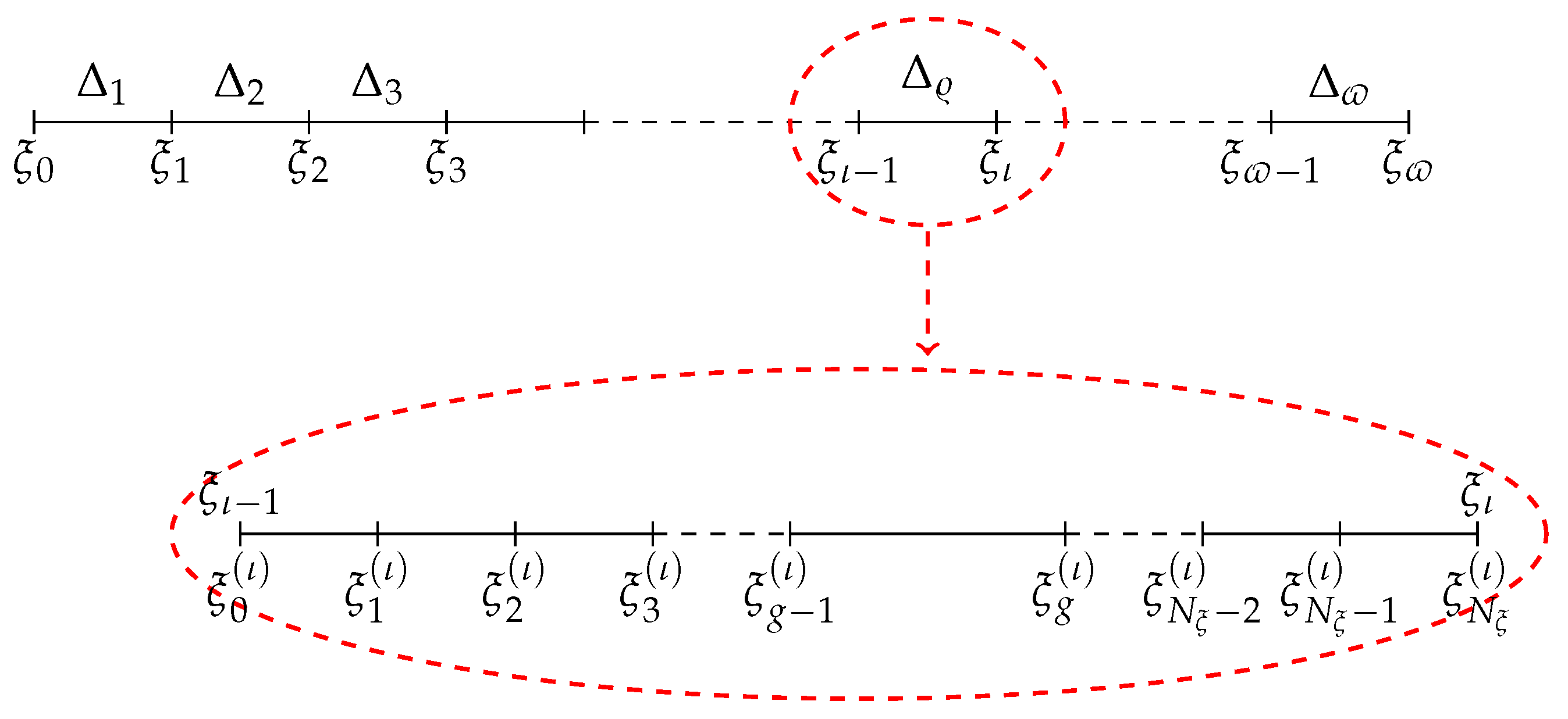
where $r+1,r$ represent current and previous iterations, and the variable coefficients have been obtained using the LLM approach (see Appendix B). The next step involves discussing the decomposition of the time domain $\xi \in [0,{\xi }_F],$ which is the solution domain for the dimensionless PDEs. The time interval $0\le \xi \le {\xi }_F$ is then segmented into $\varpi$ non-overlapping sub-domains indicated as follows:

$$\begin{array}{ccc}& & {\Delta }_{\iota }=[{\xi }_{\iota },{\xi }_{\iota -1}],0={\xi }_0<{\xi }_1<.\dots .<{\xi }_{\varpi -1}<{\xi }_{\varpi }={\xi }_F,\iota =1,2,3,\dots ,\varpi ,\hfill \end{array}$$

(31)

where each sub-domain is further partitioned into $N_{\xi }+1$ Chebyshev collocation points (see Figure 2). The PDEs are solved in the $\varpi$ non-overlapping sub-domains $[{\xi }_{\iota },{\xi }_{\iota -1}]$ by starting with the easily calculated initial solutions in the first sub-interval $\left({\Delta }_1\right)$. These initial solutions, which are initial conditions for the first interval, are obtained by solving the system of ODEs (21)–(24). For the remaining sub-domains, we use the solutions produced at the last grid point of each sub-interval as initial conditions for the next sub-interval. This means that the solution at the last grid point of ${\Delta }_{\iota }$ is used as an initial condition in ${\Delta }_{\iota +1}.$ In accordance with the validity of the spectral collocation method (SCM), which is in the interval $[-1,1],$ the decomposed domain $[{\xi }_{\iota },{\xi }_{\iota -1}]$ has to be transformed to $[-1,1]$ using the following linear transformation:

$$\begin{array}{c}\hfill \overline{\xi }=\frac{2}{{\xi }_{\iota -1}-{\xi }_{\iota }}\xi -\frac{{\xi }_{\iota }+{\xi }_{\iota -1}}{{\xi }_{\iota }-{\xi }_{\iota -1}},\xi \in [{\xi }_{\iota -1},{\xi }_{\iota }],\widehat{\xi }\in [-1,1],\iota =1,2,3,\dots ,\varpi .\end{array}$$

(32)

Because of this transformation, we now have a new collocation variable $\overline{\xi }\in [-1,1],$ which is defined as [43]

$$\begin{array}{c}\hfill {\left\{{\overline{\xi }}_j\right\}}_{j=0}^{N_{\xi }}=cos\left(\frac{j\pi }{N_{\xi }}\right).\end{array}$$

(33)

The complete grid in the time variable ($\xi$) takes the following order:

$$\begin{array}{ccc}& & \left\{0={\xi }_{N_{\xi }}^{\left(1\right)},\dots ,{\xi }_0^{\left(1\right)}={\xi }_{N_{\xi }}^{\left(2\right)},\dots ,{\xi }_0^{(\iota -1)}={\xi }_{N_{\xi }}^{\left(\iota \right)},\dots ,{\xi }_0^{\left(\varpi \right)}={\xi }_F,\dots ,2\le \iota \le \varpi \right\}.\hfill \end{array}$$

(34)

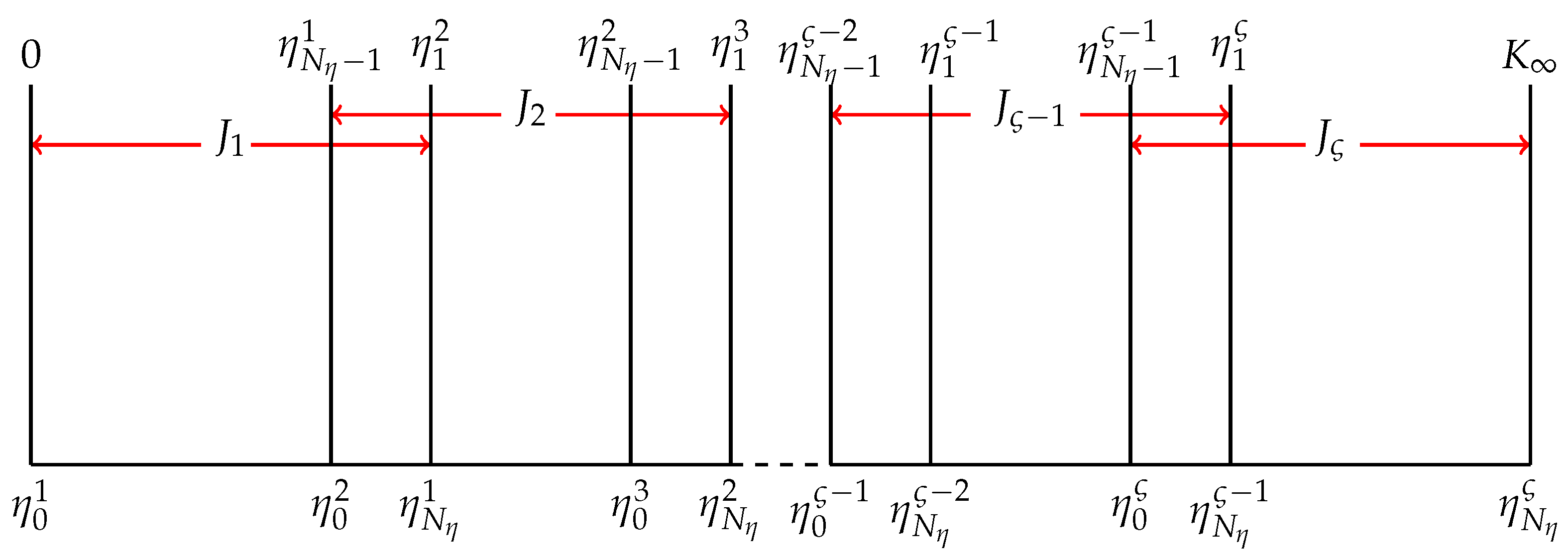
Next, we discuss domain decomposition for the spatial variable $\eta .$ Unlike the variable $\xi ,$ which is defined in the finite domain $[0,{\xi }_F],$ the space variable $\eta$ is specified in the semi-finite domain $[0,\infty ).$ In order to apply the method, this semi-finite domain has to be truncated to a finite domain $[0,K_{\infty }],$ where $K_{\infty }$ is a finite value that is handpicked with the intention that it conforms to the far field boundary constraints. The resulting truncated domain is then divided into $\varsigma$ overlapping sub-domains indicated as

$$\begin{array}{ccc}& & J_{\vartheta }=[{\eta }_0^{\left(\vartheta \right)},{\eta }_{N_{\eta }}^{\left(\vartheta \right)}],\vartheta =1,2,3,\dots ,\varsigma ,\hfill \end{array}$$

(35)

where each sub-domain is subsequently partitioned into $N_{\eta }+1$ Chebyshev collocation points (see Figure 3). Yang et al. [44] reported that using a different number of collocation points in the various sub-intervals can lead to difficulties in the implementation of the method. In addition to that condition, the length for each sub-domain must be kept the same for all sub-domains, especially if a linear transformation is utilized. This length is given by $L=\frac{K_{\infty }}{\varsigma +(1-\varsigma )(1-cos\frac{\pi }{N_{\eta }})/2}$ (see Appendix C). Again, the decomposed domain $[{\eta }_0^{\left(\vartheta \right)},{\eta }_{N_{\eta }}^{\left(\vartheta \right)}]$ has to be transformed to $[-1,1]$ as well, using the following linear mapping:

$$\begin{array}{ccc}& & \overline{\eta }=\frac{2}{{\eta }_{N_{\eta }}^{\left(\vartheta \right)}-{\eta }_0^{\left(\vartheta \right)}}\eta -\frac{{\eta }_{N_{\eta }}^{\left(\vartheta \right)}+{\eta }_0^{\left(\vartheta \right)}}{{\eta }_{N_{\eta }}^{\left(\vartheta \right)}-{\eta }_0^{\left(\vartheta \right)}},\hfill \end{array}$$

(36)

and because of this transformation, we have a new collocation variable $\overline{\eta }\in [-1,1],$ which is defined as

$$\begin{array}{ccc}& & {\left\{{\overline{\eta }}_i\right\}}_{i=0}^{N_{\eta }}=cos\left(\frac{i\pi }{N_{\eta }}\right).\hfill \end{array}$$

(37)

The complete grid in the space variable ($\eta$) takes the following order:

$$\begin{array}{c}\hfill \left\{0={\eta }_{N_{\eta }}^{\left(1\right)},\dots ,{\eta }_1^{\left(1\right)}={\eta }_{N_{\eta }}^{\left(2\right)},{\eta }_0^{\left(1\right)}={\eta }_{N_{\eta }-1}^{\left(2\right)},\dots ,{\eta }_1^{(\vartheta -1)}={\eta }_{N_{\eta }}^{\left(\vartheta \right)},{\eta }_0^{(\vartheta -1)}={\eta }_{N_{\eta }-1}^{\left(\vartheta \right)},\dots ,{\eta }_0^{\left(\varsigma \right)}=K_{\infty },2\le \vartheta \le \varsigma \right\}.\end{array}$$

(38)

The numerical solutions at different time intervals can be differentiated using $\stackrel{\left(\iota \right)}{f},\stackrel{\left(\iota \right)}{\theta },\stackrel{\left(\iota \right)}{\varphi }$, and $\stackrel{\left(\iota \right)}{\chi }.$ We remark that for the time variable, equations are solved independently in each sub-domain, but for the space variable, equations are solved contemporaneously across the whole domain of integration. Thus, the linearised iterative scheme (27)–(30) takes the form

$$\begin{array}{ccc}& & a_{0,r}\frac{{\partial }^3{\stackrel{\left(\iota \right)}{f}}_{r+1}}{\partial {\eta }^3}+a_{1,r}\frac{{\partial }^2{\stackrel{\left(\iota \right)}{f}}_{r+1}}{\partial {\eta }^2}+a_{2,r}\frac{\partial {\stackrel{\left(\iota \right)}{f}}_{r+1}}{\partial \eta }+a_{3,r}{\stackrel{\left(\iota \right)}{f}}_{r+1}+a_{4,r}\frac{\partial }{\partial \eta }\left(\frac{\partial {\stackrel{\left(\iota \right)}{f}}_{r+1}}{\partial \xi }\right)+a_{5,r}\frac{\partial {\stackrel{\left(\iota \right)}{f}}_{r+1}}{\partial \xi }=a_{6,r},\hfill \end{array}$$

(39)

$$\begin{array}{ccc}& & b_{0,r}\frac{{\partial }^2{\stackrel{\left(\iota \right)}{\theta }}_{r+1}}{\partial {\eta }^2}+b_{1,r}\frac{\partial {\stackrel{\left(\iota \right)}{\theta }}_{r+1}}{\partial \eta }+b_{2,r}{\stackrel{\left(\iota \right)}{\theta }}_{r+1}+b_{3,r}\frac{\partial {\stackrel{\left(\iota \right)}{\theta }}_{r+1}}{\partial \xi }=b_{4,r},\hfill \end{array}$$

(40)

$$\begin{array}{ccc}& & \frac{{\partial }^2{\stackrel{\left(\iota \right)}{\varphi }}_{r+1}}{\partial {\eta }^2}+c_{1,r}\frac{\partial {\stackrel{\left(\iota \right)}{\varphi }}_{r+1}}{\partial \eta }+c_{2,r}{\stackrel{\left(\iota \right)}{\varphi }}_{r+1}+c_{3,r}\frac{\partial {\stackrel{\left(\iota \right)}{\varphi }}_{r+1}}{\partial \xi }=c_{4,r},\hfill \end{array}$$

(41)

$$\begin{array}{ccc}& & \frac{{\partial }^2{\stackrel{\left(\iota \right)}{\chi }}_{r+1}}{\partial {\eta }^2}+e_{1,r}\frac{\partial {\stackrel{\left(\iota \right)}{\chi }}_{r+1}}{\partial \eta }+e_{2,r}{\stackrel{\left(\iota \right)}{\chi }}_{r+1}+e_{3,r}\frac{\partial {\stackrel{\left(\iota \right)}{\chi }}_{r+1}}{\partial \xi }=e_{4,r},\hfill \end{array}$$

(42)

In the first interval $\left({\Delta }_1\right),$ the initial conditions $\stackrel{\left(1\right)}{f}(0,\eta ),\stackrel{\left(1\right)}{\theta }(0,\eta ),\stackrel{\left(1\right)}{\varphi }(0,\eta )$, and $\stackrel{\left(1\right)}{\chi }(0,\eta )$ are used to obtained numerical solutions $\stackrel{\left(1\right)}{f}(\xi ,\eta ),\stackrel{\left(1\right)}{\theta }(\xi ,\eta ),\stackrel{\left(1\right)}{\varphi }(\xi ,\eta )$, and $\stackrel{\left(1\right)}{\chi }(\xi ,\eta ).$ Then, for the remaining time sub-intervals $({\Delta }_{\iota },\iota =2,3,4,\dots ,\varpi )$, the continuity conditions are given as

$$\begin{array}{ccc}& & {\stackrel{\left(\iota \right)}{f}}_{r+1}({\xi }_{\iota -1},\eta )={\stackrel{(\iota -1)}{f}}_{r+1}({\xi }_{\iota -1},\eta ),{\stackrel{\left(\iota \right)}{\theta }}_{r+1}({\xi }_{\iota -1},\eta )={\stackrel{(\iota -1)}{\theta }}_{r+1}({\xi }_{\iota -1},\eta ),\hfill \end{array}$$

(43)

$$\begin{array}{ccc}& & {\stackrel{\left(\iota \right)}{\varphi }}_{r+1}({\xi }_{\iota -1},\eta )={\stackrel{(\iota -1)}{\varphi }}_{r+1}({\xi }_{\iota -1},\eta ),{\stackrel{\left(\iota \right)}{\chi }}_{r+1}({\xi }_{\iota -1},\eta )={\stackrel{(\iota -1)}{\chi }}_{r+1}({\xi }_{\iota -1},\eta ),\hfill \end{array}$$

(44)

are used to generate numerical solutions $\stackrel{\left(\iota \right)}{f}(\xi ,\eta ),\stackrel{\left(\iota \right)}{\theta }(\xi ,\eta ),\stackrel{\left(\iota \right)}{\varphi }(\xi ,\eta )$, and $\stackrel{\left(\iota \right)}{\chi }(\xi ,\eta )(\iota =2,3,\dots ,\varpi )$ in the other sub-intervals. The procedure for generating the numerical solution is carried out by approximating the desired solutions, such as $f(\xi ,\eta )$, using the bivariate Lagrange interpolating polynomial that appears as

$$\begin{array}{c}\hfill \stackrel{\left(\iota \right)}{f}(\xi ,\eta )\approx \stackrel{\left(\iota \right)}{F}(\xi ,\eta )=\sum _{h=0}^{N_{\eta }}\sum _{l=0}^{N_{\xi }}\stackrel{\left(\iota \right)}{F}({\eta }_h,{\xi }_l)L_h\left(\eta \right)L_l\left(\xi \right).\end{array}$$

(45)

For each space sub-domain $J_{\vartheta }$, the first, second, and $n^{th}$ order derivative matrices in the spatial direction are evaluated at the collocation points $({\overline{\xi }}_i,{\overline{\eta }}_j)$ for $j=0,1,2,\dots ,N_{\xi }$ as follows [33]:

$$\begin{array}{ccc}& & \frac{\partial \stackrel{\left(\iota \right)}{f}}{\partial \eta }({\overline{\eta }}_i,{\xi }_j)=\mathbf{D}{\stackrel{\left(\iota \right)}{\mathbf{F}}}_j,\frac{{\partial }^2\stackrel{\left(ϵ\right)}{f}}{\partial {\eta }^2}({\overline{\eta }}_i,{\xi }_j)={\mathbf{D}}^2{\stackrel{\left(\iota \right)}{\mathbf{F}}}_j,\frac{{\partial }^n\stackrel{\left(ϵ\right)}{f}}{\partial {\eta }^n}({\overline{\eta }}_i,{\xi }_j)={\mathbf{D}}^n{\stackrel{\left(\iota \right)}{\mathbf{F}}}_j,\hfill \end{array}$$

(46)

where the Chebyshev differential matrix $\mathbf{D}=\frac{2}{L}\overline{\mathbf{D}},$ and $\overline{\mathbf{D}}$ in the standard Chebyshev differential matrix of the first order with dimension $(N_{\eta }+1)\times (N_{\eta }+1).$ However, the matrix $\mathbf{D}$ has dimension $(M_{\eta }+1)\times (M_{\eta }+1),$ where $M_{\eta }=N_{\eta }+(N_{\eta }-1)(\varsigma -1)$ is the combination of all collocation points used in the whole spatial region. On the other hand, ${\stackrel{\left(\iota \right)}{\mathbf{F}}}_j={\left[\stackrel{\left(\iota \right)}{f}({\eta }_0^{\left(\vartheta \right)},{\xi }_j),\stackrel{\left(\iota \right)}{f}({\eta }_1^{\left(\vartheta \right)},{\xi }_j),\stackrel{\left(\iota \right)}{f}({\eta }_2^{\left(\vartheta \right)},{\xi }_j),\dots ,\stackrel{\left(\iota \right)}{f}({\eta }_{N_{\eta }}^{\left(\vartheta \right)},{\xi }_j)\right]}^T$ is the matrix-vector function with dimension $(N_{\eta }+1)\times 1.$ We note that the $n^{th}(n>1)$ derivative matrix is obtained via matrix multiplication. For each time sub-interval ${\Delta }_{\iota }$, the first-order derivative matrix in the time direction is evaluated at the collocation points $({\overline{\xi }}_i,{\overline{\eta }}_j)$ for $i=0,1,2,3,\dots ,N_{\eta }$ as [33]

$$\begin{array}{ccc}& & \frac{\partial \stackrel{\left(\iota \right)}{f}}{\partial \xi }({\overline{\eta }}_i,{\xi }_j)=\sum _{l=0}^{N_{\xi }}{d}_{j,l}{\stackrel{\left(\iota \right)}{\overline{\mathbf{F}}}}_l\hfill \end{array}$$

(47)

where $d_{j,l}=\frac{2}{{\xi }_{\iota }-{\xi }_{\iota -1}}{\overline{d}}_{j,l}(j,l=0,1,2,3,\dots ,N_{\xi }),$ and ${\overline{d}}_{j,l}$ in the standard Chebyshev differential matrix of the first order with dimension $(N_{\xi }+1)\times (N_{\xi }+1).$ It is noteworthy that the matrix-vector function ${\stackrel{\left(\iota \right)}{\overline{\mathbf{F}}}}_l$ has dimension $(M_{\eta }+1)\times 1$, since it accounts for the solution in the entire spatial domain. A similar procedure is utilized in the approximation of the other unknown functions $\theta (\xi ,\eta ),\varphi (\xi ,\eta ),\chi (\xi ,\eta )$, and their corresponding derivatives at the collocation points $({\overline{\xi }}_i,{\overline{\eta }}_j)$. Because of the execution of the overlapping grid strategy, the Chebyshev differential matrix $\mathbf{D}$ contains many zero elements and becomes less dense, and the structure of the matrix is illustrated in [32,33,38,39] (see Appendix D). The crucial idea behind the use of SCM lies in the approximation of continuous derivatives with discrete derivatives. Consequently, by replacing the continuous derivatives in Equations (39)–(42) with the discrete derivatives discussed in the previous paragraphs and making use of the initial conditions, we obtain

$$\begin{array}{ccc}& & \left[{\mathit{a}}_{0,r}{\mathbf{D}}^3+{\mathit{a}}_{1,r}{\mathbf{D}}^2+{\mathit{a}}_{2,r}\mathbf{D}+{\mathit{a}}_{3,r}\right]{\stackrel{\left(\iota \right)}{\overline{\mathbf{F}}}}_{i,r+1}+{\mathit{a}}_{4,r}\sum _{j=0}^{N_{\xi -1}}{d}_{i,j}\mathbf{D}{\stackrel{\left(\iota \right)}{\overline{\mathbf{F}}}}_{j,r+1}+{\mathit{a}}_{5,r}\sum _{j=0}^{N_{\xi -1}}{d}_{i,j}{\stackrel{\left(\iota \right)}{\overline{\mathbf{F}}}}_{j,r+1}={\stackrel{\left(\iota \right)}{\mathbf{R}}}_{1,i,r},\hfill \end{array}$$

(48)

$$\begin{array}{ccc}& & \left[{\mathit{b}}_{0,r}{\mathbf{D}}^2+{\mathit{b}}_{1,r}\mathbf{D}+{\mathit{b}}_{2,r}\right]{\stackrel{\left(\iota \right)}{\overline{\mathsf{\Theta }}}}_{i,r+1}+{\mathit{b}}_{3,r}\sum _{j=0}^{N_{\xi -1}}{d}_{i,j}{\stackrel{\left(\iota \right)}{\overline{\mathsf{\Theta }}}}_{j,r+1}={\stackrel{\left(\iota \right)}{\mathbf{R}}}_{2,i,r},\hfill \end{array}$$

(49)

$$\begin{array}{ccc}& & \left[{\mathbf{D}}^2+{\mathit{c}}_{1,r}\mathbf{D}+{\mathit{c}}_{2,r}\right]{\stackrel{\left(\iota \right)}{\overline{\mathsf{\Phi }}}}_{i,r+1}+{\mathit{c}}_{3,r}\sum _{j=0}^{N_{\xi -1}}{d}_{i,j}{\stackrel{\left(\iota \right)}{\overline{\mathsf{\Phi }}}}_{j,r+1}={\stackrel{\left(\iota \right)}{\mathbf{R}}}_{3,i,r},\hfill \end{array}$$

(50)

$$\begin{array}{ccc}& & \left[{\mathbf{D}}^2+{\mathit{e}}_{1,r}\mathbf{D}+{\mathit{e}}_{2,r}\right]{\stackrel{\left(\iota \right)}{\overline{\mathsf{\chi }}}}_{i,r+1}+{\mathit{e}}_{3,r}\sum _{j=0}^{N_{\xi -1}}{d}_{i,j}{\stackrel{\left(\iota \right)}{\overline{\mathsf{\chi }}}}_{j,r+1}={\stackrel{\left(\iota \right)}{\mathbf{R}}}_{4,i,r},\hfill \end{array}$$

(51)

where the right-hand side of the equations are explicated as ${\stackrel{\left(\iota \right)}{\mathbf{R}}}_{1,i,r}={\mathit{a}}_{6,r}-{\mathit{a}}_{4,r}{d}_{i,N_{\xi }}\mathbf{D}{\stackrel{\left(\iota \right)}{\overline{\mathbf{F}}}}_{N_{\xi }}-{\mathit{a}}_{5,r}{d}_{i,N_{\xi }}{\stackrel{\left(\iota \right)}{\overline{\mathbf{F}}}}_{N_{\xi }},$${\stackrel{\left(\iota \right)}{\mathbf{R}}}_{2,i,r}={\mathit{b}}_{4,r}-{\mathit{b}}_{3,r}{d}_{i,N_{\xi }}{\stackrel{\left(\iota \right)}{\overline{\mathsf{\Theta }}}}_{N_{\xi }},{\stackrel{\left(\iota \right)}{\mathbf{R}}}_{3,i,r}={\mathit{c}}_{4,r}-{\mathit{c}}_{3,r}{d}_{i,N_{\xi }}{\stackrel{\left(\iota \right)}{\overline{\mathsf{\Phi }}}}_{N_{\xi }},$ and ${\stackrel{\left(\iota \right)}{\mathbf{R}}}_{4,i,r}={\mathit{e}}_{4,r}-{\mathit{e}}_{3,r}{d}_{i,N_{\xi }}{\stackrel{\left(\iota \right)}{\overline{\mathsf{\chi }}}}_{N_{\xi }}.$ The matching boundary constraints are also evaluated at the collocation points, and they take the form

$$\begin{array}{ccc}& & {\stackrel{\left(\iota \right)}{f}}_{r+1}({\eta }_{M_{\eta }},{\xi }_i)=f_w,\sum _{h=0}^{M_{\eta }}{\mathbf{D}}_{M_{\eta },h}{\stackrel{\left(\iota \right)}{f}}_{r+1}({\eta }_h,{\xi }_i)-\delta \sum _{h=0}^{M_{\eta }}{\mathbf{D}}_{M_{\eta },h}^2{\stackrel{\left(\iota \right)}{f}}_{r+1}({\eta }_h,{\xi }_i)=0,{\stackrel{\left(\iota \right)}{\chi }}_{r+1}({\eta }_{M_{\eta }},{\xi }_i)=1,\hfill \\ & & \sum _{h=0}^{M_{\eta }}{\mathbf{D}}_{M_{\eta },h}{\stackrel{\left(\iota \right)}{f}}_{r+1}({\eta }_h,{\xi }_i)-Bi{\stackrel{\left(\iota \right)}{\theta }}_{r+1}({\eta }_{M_{\eta }},{\xi }_i)=-Bi,\hfill \\ & & \sum _{h=0}^{M_{\eta }}{\mathbf{D}}_{M_{\eta },h}{\stackrel{\left(\iota \right)}{\varphi }}_{r+1}({\eta }_h,{\xi }_i)+\frac{Nt}{Nb}\sum _{h=0}^{M_{\eta }}{\mathbf{D}}_{M_{\eta },h}^2{\stackrel{\left(\iota \right)}{\theta }}_{r+1}({\eta }_h,{\xi }_i)=0,\hfill \\ & & \sum _{h=0}^{M_{\eta }}{\mathbf{D}}_{0,h}{\stackrel{\left(\iota \right)}{f}}_{r+1}({\eta }_h,{\xi }_i)=\frac{sin{\xi }_i}{{\xi }_i},{\stackrel{\left(\iota \right)}{\theta }}_{r+1}({\eta }_0,{\xi }_i)=0,{\stackrel{\left(\iota \right)}{\varphi }}_{r+1}({\eta }_0,{\xi }_i)=0,{\stackrel{\left(\iota \right)}{\chi }}_{r+1}({\eta }_0,{\xi }_i)=0.\hfill \end{array}$$

(52)

In the form of an $N_{\xi }(M_{\eta }+1)\times N_{\xi }(M_{\eta }+1)$ matrix arrangement, Equation (48) takes the form

$${\displaystyle \left[\begin{array}{ccccc}{\mathbf{A}}_{0,0}& {\mathbf{A}}_{0,1}& {\mathbf{A}}_{0,2}& \cdots & {\mathbf{A}}_{0,N_{\xi }-1}\\ {\mathbf{A}}_{1,0}& {\mathbf{A}}_{1,1}& {\mathbf{A}}_{1,2}& \cdots & {\mathbf{A}}_{1,N_{\xi }-1}\\ ⋮& ⋮& \ddots & ⋮\\ {\mathbf{A}}_{N_{\xi }-1,0}& {\mathbf{A}}_{N_{\xi }-1,1}& {\mathbf{A}}_{N_{\xi }-1,2}& \cdots & {\mathbf{A}}_{N_{\xi }-1,N_{\xi }-1}\end{array}\right]}{\displaystyle \left[\begin{array}{c}{\stackrel{\left(\iota \right)}{\overline{\mathbf{F}}}}_0\\ {\stackrel{\left(\iota \right)}{\overline{\mathbf{F}}}}_1\\ ⋮\\ {\stackrel{\left(\iota \right)}{\overline{\mathbf{F}}}}_{N_{\xi }-1}\end{array}\right]=\left[\begin{array}{c}{\stackrel{\left(\iota \right)}{\mathbf{R}}}_{1,0}\\ {\stackrel{\left(\iota \right)}{\mathbf{R}}}_{1,1}\\ ⋮\\ {\stackrel{\left(\iota \right)}{\mathbf{R}}}_{1,N_{\xi }-1}\end{array}\right]},$$

(53)

where

$$\begin{array}{ccc}& & {\mathbf{A}}_{i,i}={\mathit{a}}_{0,r}{\mathbf{D}}^3+{\mathit{a}}_{1,r}{\mathbf{D}}^2+{\mathit{a}}_{2,r}\mathbf{D}+{\mathit{a}}_{3,r}\mathbf{I}+{\mathit{a}}_{4,r}{d}_{i,i}\mathbf{D}+{\mathit{a}}_{5,r}{d}_{i,i}\mathbf{I},i=j,\hfill \\ & & {\mathbf{A}}_{i,j}^{\left(1\right)}={\mathit{a}}_{4,r}{d}_{i,j}\mathbf{D}+{\mathit{a}}_{5,r}{d}_{i,j}\mathbf{I},i\ne j,\hfill \end{array}$$

(54)

$${\displaystyle \left[\begin{array}{ccccc}{a}_{\zeta ,r}({\eta }_0,{\xi }_i)& & & & \\ & a_{\zeta ,r}({\eta }_1,{\xi }_i)& & & \\ & & \ddots & \\ & & & & a_{\zeta ,r}({\eta }_{M_{\eta }},{\xi }_i)\end{array}\right]},\zeta =0,1,2,3,4,5,$$

(55)

and $\mathbf{I}$ is an $(M_{\eta }+1)\times (M_{\eta }+1)$ unit matrix. The additional equations will also give a similar matrix arrangement of the same dimension. The resulting discrete boundary conditions are incorporated into the main diagonal sub-blocks of each matrix system to yield a new system of linear algebraic equations. The later matrix system is then solved iteratively, resuming with initial approximations that are picked in such a way that they conform to the boundary conditions. The compact form of matrix Equations (48)–(51) is given by

$${\displaystyle \left[\begin{array}{c}\stackrel{\left(1\right)}{\mathbf{A}}\end{array}\right]}{\displaystyle \left[\begin{array}{c}\mathbf{F}\end{array}\right]}={\displaystyle \left[\begin{array}{c}{\mathbf{R}}_1\end{array}\right]},{\displaystyle \left[\begin{array}{c}\stackrel{\left(2\right)}{\mathbf{A}}\end{array}\right]}{\displaystyle \left[\begin{array}{c}\mathsf{\Theta }\end{array}\right]}={\displaystyle \left[\begin{array}{c}{\mathbf{R}}_2\end{array}\right]},{\displaystyle \left[\begin{array}{c}\stackrel{\left(3\right)}{\mathbf{A}}\end{array}\right]}{\displaystyle \left[\begin{array}{c}\mathsf{\Phi }\end{array}\right]}={\displaystyle \left[\begin{array}{c}{\mathbf{R}}_3\end{array}\right]},{\displaystyle \left[\begin{array}{c}\stackrel{\left(4\right)}{\mathbf{A}}\end{array}\right]}{\displaystyle \left[\begin{array}{c}\mathsf{\chi }\end{array}\right]}={\displaystyle \left[\begin{array}{c}{\mathbf{R}}_4\end{array}\right]}.$$

(56)

The functions used as initial guesses are given by

$$f_0\left(\eta \right)=f_w+\frac{1}{1+\delta }\left(e^{-\eta }-1\right)+\eta ,{\theta }_0\left(\eta \right)=\frac{Bi}{1+Bi}{e}^{-\eta },{\varphi }_0\left(\eta \right)=-\frac{NtBi}{Nb(1+Bi)}{e}^{-\eta },{\chi }_0\left(\eta \right)=e^{-\eta }.$$

(57)

4. Results and Discussion

A comprehensive parametric study is carried out and numerical results are reported in this section through graphs. The numerical computation is performed for each parameter by assigning fixed values to other related parameters as $\xi =\frac{\pi }{2}$ [13,28], $\omega =0.2$ [28], $Rb=0.1$ [28],$Nt=0.1$ [13,28], $Nb=0.3$ [13,28], $Sc=10$ [13,28], $Pe=1$ [28], $Sb=1$ [28], $Nr=0.5$ [13,28], $Pr=6.8$ [28], $\delta =0.5$ [4], $K_c=2$ [18], $Bi=5$ [13,28], $K_m=2,M=0.5$ [4,17], $f_w$ [18]$=0.5,Rd=0.5$ [17], ${\theta }_f=1.1$ [16], $\mathsf{\Lambda }=1$ [17], $\epsilon =1$ [28], $\beta =0.5$ [37], $Q=0.2$ [37], $\alpha =0.3$ [39], $E=2$ [18], $p=0.2$ [18], $\mathsf{\Omega }=0.1$ [17], $\lambda =5$ [13,28], and $Nn=0.2$ [29]. To corroborate the correctness of the present numerical method, the results for the heat transfer rate $-{\theta }^{\prime }\left(0\right)$ were contrasted against those disclosed by Merkin [15], Nazar et al. [1], Rashad et al. [13], Rashad et al. [28], and Zahar et al. [16] in

Table 1. Comparison of $-{\theta }^{\prime }\left(0\right)$ when $Pr=1,{\theta }_f=1,Bi\to \infty ,\xi =\beta =\alpha =f_w=M=\mathsf{\Lambda }=Rd=$ $Q=\epsilon =\delta =Nr=Rb=\mathsf{\Omega }=Nb=Nn=Nt=Sc=Sb=E=K_c=Pe=K_m=\omega =p=0.$

$\mathit{\lambda }$	Merkin [15]	Nazar et al. [1]	Rashad et al.  [13]	Rashad et al. [28]	Zahar et al. [16]	Present Results
−1.75	0.4199	0.4205	0.4202	0.4202	0.4198	0.4199516
−1.50	0.4576	0.4601	0.4579	0.4579	0.4573	0.4573551
−1.00	0.5067	0.5080	0.5068	0.5068	0.5067	0.5066785
−0.50	0.5420	0.5430	0.5421	0.54201	0.5421	0.5420654
0.00	0.5705	0.5710	0.5706	0.5706	0.5705	0.5704700
0.50	0.5943	0.5949	0.5947	0.5947	0.5945	0.5945339
0.88	0.6096	0.6112	0.6111	0.6111	0.6108	0.6107615
0.89	0.6110	0.6116	0.6114	0.6114	0.6112	0.6111687
1.00	0.6158	0.6160	0.6160	0.6160	0.6154	0.6155872
2.00	0.6497	0.6518	0.6518	0.6518	0.6515	0.6514920
5.00	0.7315	0.7320	0.7319	0.7319	0.7315	0.7315104

. Table 1 demonstrates that the numerical values in all considered cases were in substantial coherence. Hence, the selection of the present overlapping grid-based numerical scheme can be rationalized.

The convergence of the OMD-BSLLM is tracked by monitoring the solution errors, as defined in [32]. These errors represent solution-based discrepancies and quantify the number of accurate digits in the approximate solutions at the r-th iteration level. If the numerical scheme is converging, it is anticipated that the error norms will decrease as the number of iterations increases. Figure 4 illustrates the evolution of the solution errors for the approximate numerical solutions of $f(\eta ,\xi ),\theta (\eta ,\xi ),\varphi (\eta ,\xi ),$ and $\chi (\eta ,\xi )$ over iterations in both MD-BSLLM and OMD-BSLLM. The consistent reduction in all solution errors suggests that the numerical methods converge. Full convergence is considered attained when the convergence plots start to level off. It is evident that complete convergence is reached after approximately five iterations for all solutions in the MD-BSLLM approach and six iterations for all solutions in the OMD-BSLLM technique, with solution errors approaching ${10}^{-8}$ and ${10}^{-12}$ in the MD-BSLLM scheme and OMD-BSLLM technique, respectively. The minimal errors observed with the OMD-BSLLM approach validate its superior accuracy compared to the MD-BSLLM scheme. The precision of the overlapping grid-based scheme (OMD-BSLLM) can be assessed by evaluating the residual errors, as defined in [32]. 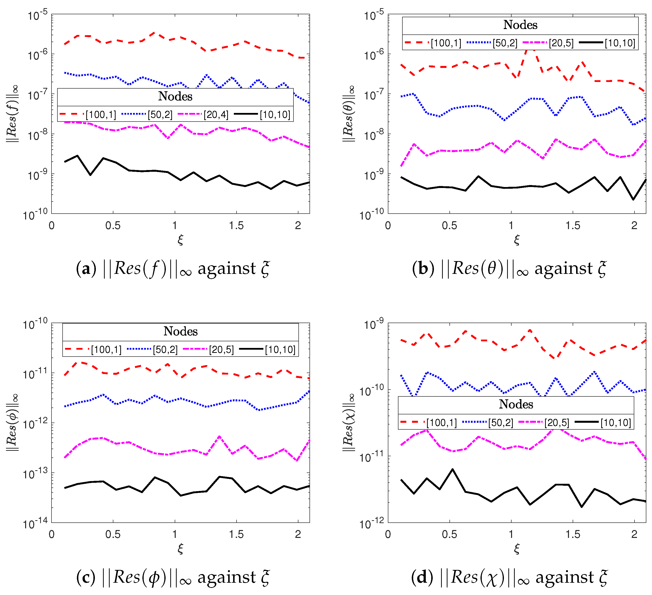These errors quantify how closely the numerical solutions approximate the true solution of the PDEs (16)–(19). Figure 5 is plotted to demonstrate residual error graphs at different time levels for both OMD-BSLLM and MD-BSLLM (no overlapping) schemes. In all the graphs, it is clear that each graph displays sufficiently small residual errors, and that is an indication of good accuracy in both numerical schemes. The accuracy is also noted to be uniform throughout the time domain, and that is one of the benefits of using the multi-domain approach in the implementation of SCM. Nevertheless, the OMD-BSLLM scheme proves to be more accurate than the MD-BSLLM approach in all the graphs. Furthermore, using more overlapping sub-domains with a smaller number of spatial collocation points yields more precision in the OMD-BSLLM approach.

The stability of the OMD-BSLLM scheme is assessed by analyzing the condition numbers of the coefficient matrices associated with the system of linear algebraic equations that need to be solved. The condition number of the matrix gauges the degree of sensitivity of the solution to variations in the input data and to the round-off errors incurred during the solution process. The condition numbers for the coefficient matrices $(\stackrel{\left(1\right)}{\mathbf{A}},\stackrel{\left(2\right)}{\mathbf{A}},\stackrel{\left(3\right)}{\mathbf{A}},\stackrel{\left(4\right)}{\mathbf{A}})$ are presented in

Table 2. Condition numbers for varying nodes $[N_{\eta },\varsigma ]$.

$\mathit{\varsigma }$	${\mathit{N}}_{\mathit{\eta }}$	${\mathit{M}}_{\mathit{\eta }}$	$\mathbf{Cond}\mathbf{(}\stackrel{\mathbf{\left(}\mathbf{1}\mathbf{\right)}}{\mathbf{A}}\mathbf{)}$	$\mathbf{Cond}\mathbf{(}\stackrel{\mathbf{\left(}\mathbf{2}\mathbf{\right)}}{\mathbf{A}}\mathbf{)}$	$\mathbf{Cond}\mathbf{(}\stackrel{\mathbf{\left(}\mathbf{3}\mathbf{\right)}}{\mathbf{A}}\mathbf{)}$	$\mathbf{Cond}\mathbf{(}\stackrel{\mathbf{\left(}\mathbf{4}\mathbf{\right)}}{\mathbf{A}}\mathbf{)}$
1 (MD-BSLLM)	100	100	1.4518640e+10	6.0399799e+06	2.5107303e+06	3.1173003e+06
2 (OMD-BSLLM)	50	99	1.7962336e+09	1.2883089e+06	5.4063508e+05	6.6439084e+05
4 (OMD-BSLLM)	25	97	2.4075014e+08	2.7726519e+05	1.1971839e+05	1.4291087e+05
5 (OMD-BSLLM)	20	96	1.2646992e+08	1.6967207e+05	7.4692771e+04	8.7440012e+04
10 (OMD-BSLLM)	10	91	1.6621778e+07	3.7796142e+04	1.9268267e+04	1.9579885e+04
20 (OMD-BSLLM)	5	81	1.7880098e+06	9.4107769e+03	7.4254531e+03	4.6950726e+03
25 (OMD-BSLLM)	4	76	8.0984196e+05	6.3770832e+03	6.1905704e+03	2.9795539e+03

when the number of collocation points and overlapping sub-intervals are varied. The overlapping grid-based numerical scheme is noted to yield small condition numbers compared to the non-overlapping grid-based scheme. The use of the overlapping grid approach results in coefficient matrices that are better conditioned compared to those generated by the non-overlapping grid-based calculations. The small condition numbers observed with the overlapping grid-based scheme indicate that the problem is well-conditioned, suggesting that the matrix representing the problem is not close to being singular. This characteristic is desirable as it ensures the stability, accuracy, and reliability of the numerical solution to the problem. As the number of overlapping sub-intervals increases and the number of space collocation points decreases, the condition numbers also decrease. This trend suggests that maximizing the number of overlapping sub-intervals while reducing the number of space collocation points further enhances the stability and accuracy of the numerical solutions. These findings affirm that the OMD-BSLLM scheme is the preferred numerical method for solving fluid flow problems akin to the one addressed in the current study.

For brevity, the consequences of other flow parameters such as $\epsilon ,Bi,Nr,\mathsf{\Lambda },Rb,Nb,Nt,$$Pe,Pr,Sc,$ and $Sb$ on the fluid flow attributes and design quantities of engineering attentiveness have been omitted in the current study. This is because the contributions of these flow parameters are similar to the ones that were adequately discussed in Rashid et al. [13,28] in the scenario of Newtonian fluids and the absence of variable fluid properties, nonlinear heat convection, magnetic field, heat sink/source, nonlinear thermal radiation, bioconvection Brownian diffusion, activation energy, chemical and microbial reactions, suction/injection, and first-order velocity slips. The current study seeks to extend the works of Rashid et al. [13,28] by analyzing, from a mathematical point of view, the fluid flow properties, heat, mass, and motile microbe transfer phenomena when the above features are incorporated in the present bioconvection flow model. Figure 6, Figure 7, Figure 8, Figure 9, Figure 10, Figure 11, Figure 12, Figure 13, Figure 14, Figure 15, Figure 16, Figure 17, Figure 18, Figure 19 and Figure 20 illustrate the impact of various parameters stemming from the aforementioned novel features, including the Williamson fluid $\left(\mathsf{\Lambda }\right)$, nonlinear convection $\left(\mathsf{\Omega }\right)$, suction $(f_w>0)$, velocity slip $\left(\delta \right)$, variable viscosity $\left(\alpha \right)$, magnetic field $\left(M\right)$, thermal radiation $\left(Rd\right)$, temperature ratio $\left({\theta }_f\right)$, variable thermal conductivity $\left(\beta \right)$, heat source $(Q>0)$, chemical reaction $\left(K_c\right)$, AE $\left(E\right)$, microbial reaction $\left(K_m\right)$, microbial Brownian motion $\left(Nn\right)$, and motile microbe $\left(\omega \right)$ parameters, on dimensionless velocity $\left(f^{\prime }\right)$, temperature $\left(\theta \right)$, NP concentration $\left(\varphi \right)$, density of motile microbes $\left(\chi \right)$, wall friction factor $\left(C_f\right)$, Nusselt number $\left(Nu\right)$, and density number of motile microbes $\left(Nm\right)$. These pertinent parameters are chosen in the ranges: $\mathsf{\Lambda }$ = 0, 1, 2, 3; $\mathsf{\Omega }$ = 0.1, 0.5, 1, 1.5; $f_w$ = 0.1, 0.3, 0.5, 0.8; $\delta$ = 0.1, 0.3, 0.5, 0.8; $\alpha$ = 0.1, 0.5, 1, 1.5; M = 0.1, 1, 5, 10; $Rd$ = 0.3, 0.6, 1, 1.5; ${\theta }_f$ = 1.1, 1.3, 1.5, 1.8; 0.1, 0.5, 1, 1.5; Q = 0.1, 0.3, 0.5, 0.8; $K_c$ = 0.1, 1, 2, 3, 5; E = 0, 1, 2, 3; $K_m$ = 0.1, 1, 3, 5; $Nn$ = 0.2, 0.3, 0.5, 0.8; and $\omega$ = 0.1, 0.3, 0.5, 0.8. The selected range of values for the present model align with those commonly found in a typical nanofluid. For parameters exhibiting a broad spectrum, we opted for values that ensured the stability of the numerical scheme. 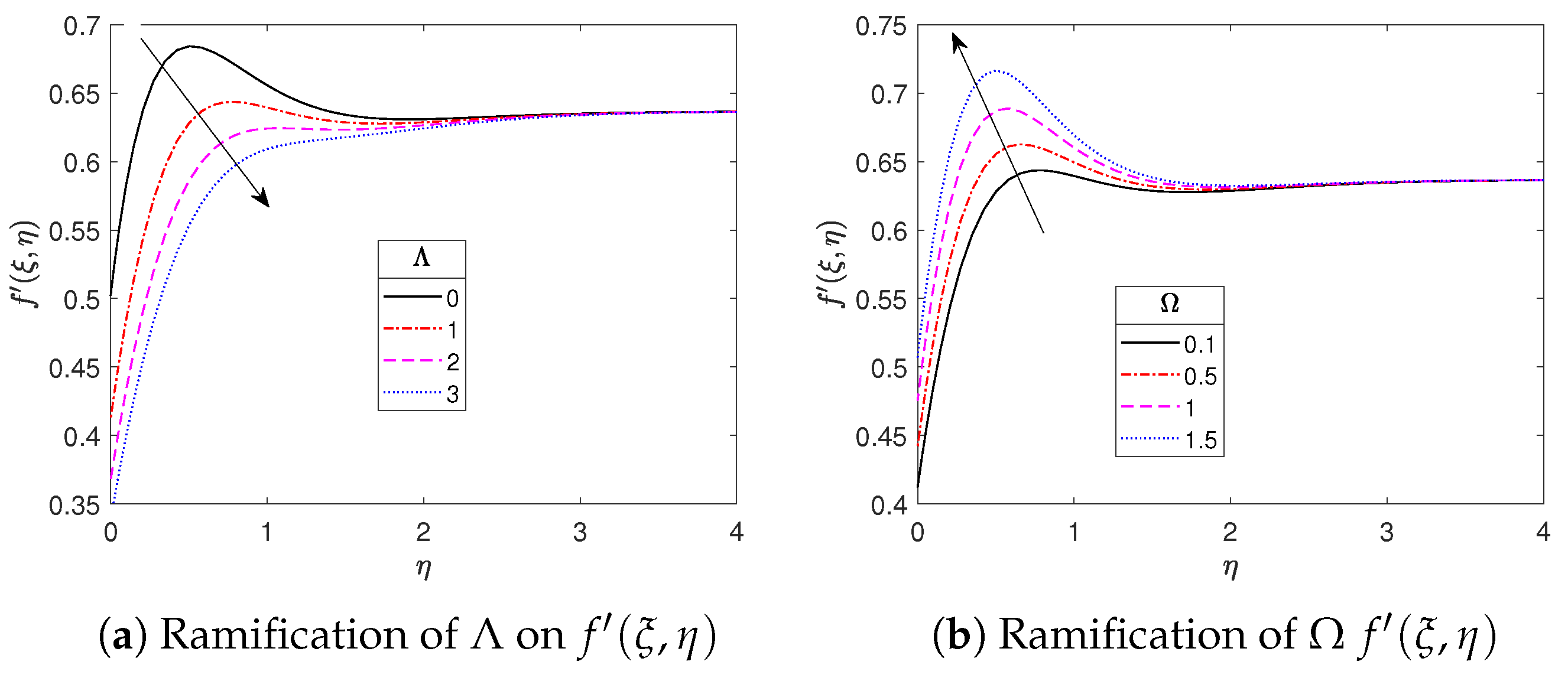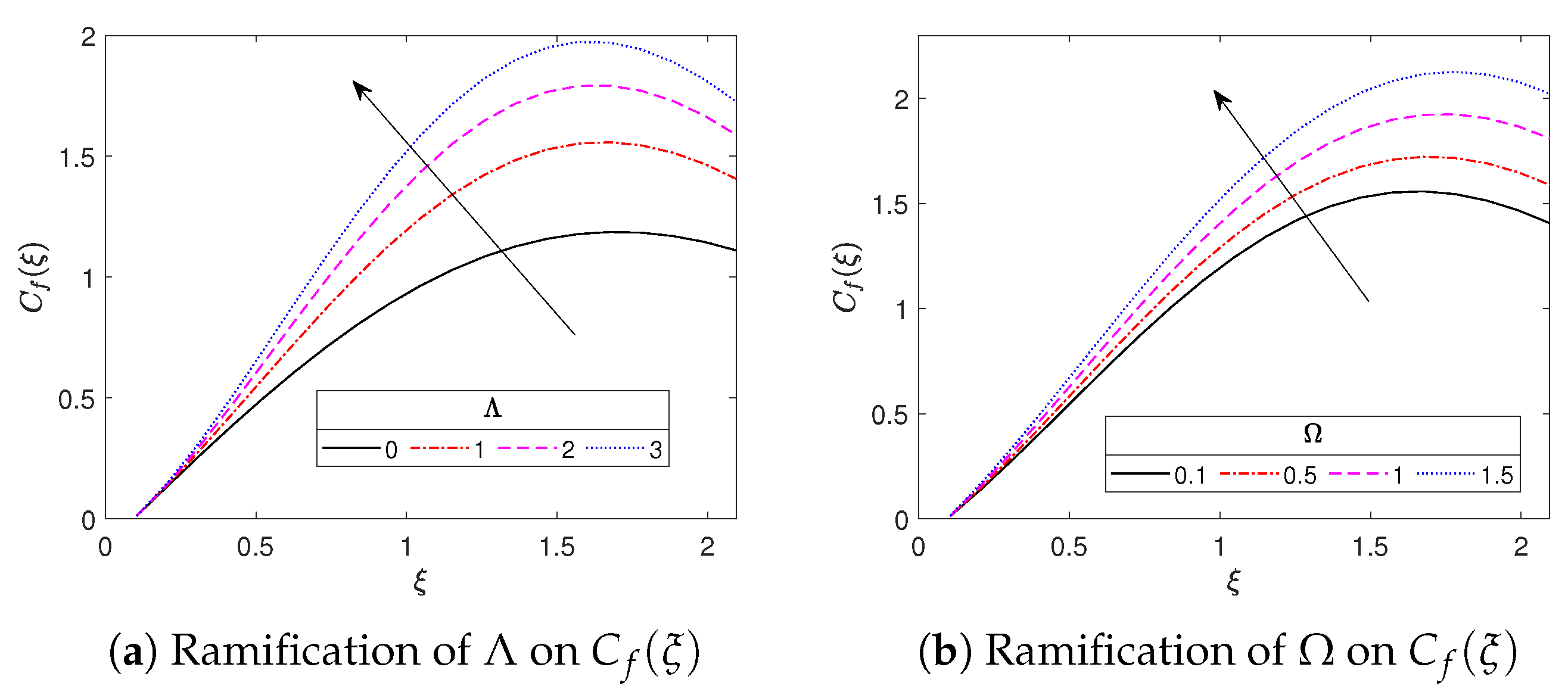Figure 6 is plotted to demonstrate the impact of the Williamson fluid parameter $\left(\mathsf{\Lambda }\right)$ and nonlinear thermal convection parameter $\left(\mathsf{\Omega }\right)$ on the dimensionless velocity. From Figure 6a, it is clear that velocity dissemination is diminished with increasing values of $\mathsf{\Lambda }.$ The variable $\mathsf{\Lambda }$ signifies the ratio of Williamson fluid relaxation time to retardation time. When the Williamson fluid parameter gets larger, the relaxation time of the fluid is noted to be lifted. As a result, resistance in the fluid flow direction is produced, which in turn reduces the NF velocity. Basically, because of the high relaxation time, fluid particles take more time to migrate to their original position; thus, fluid viscosity is improved and the velocity of the fluid particles is diminished. Conversely, velocity dissemination is accelerated with mounting values of $\mathsf{\Omega }$. For larger $\mathsf{\Omega }$, the disparity between the surface and free stream (ambient) temperatures $(T_f-T_{\infty })$ is increased, instigating a rise in the fluid velocity.

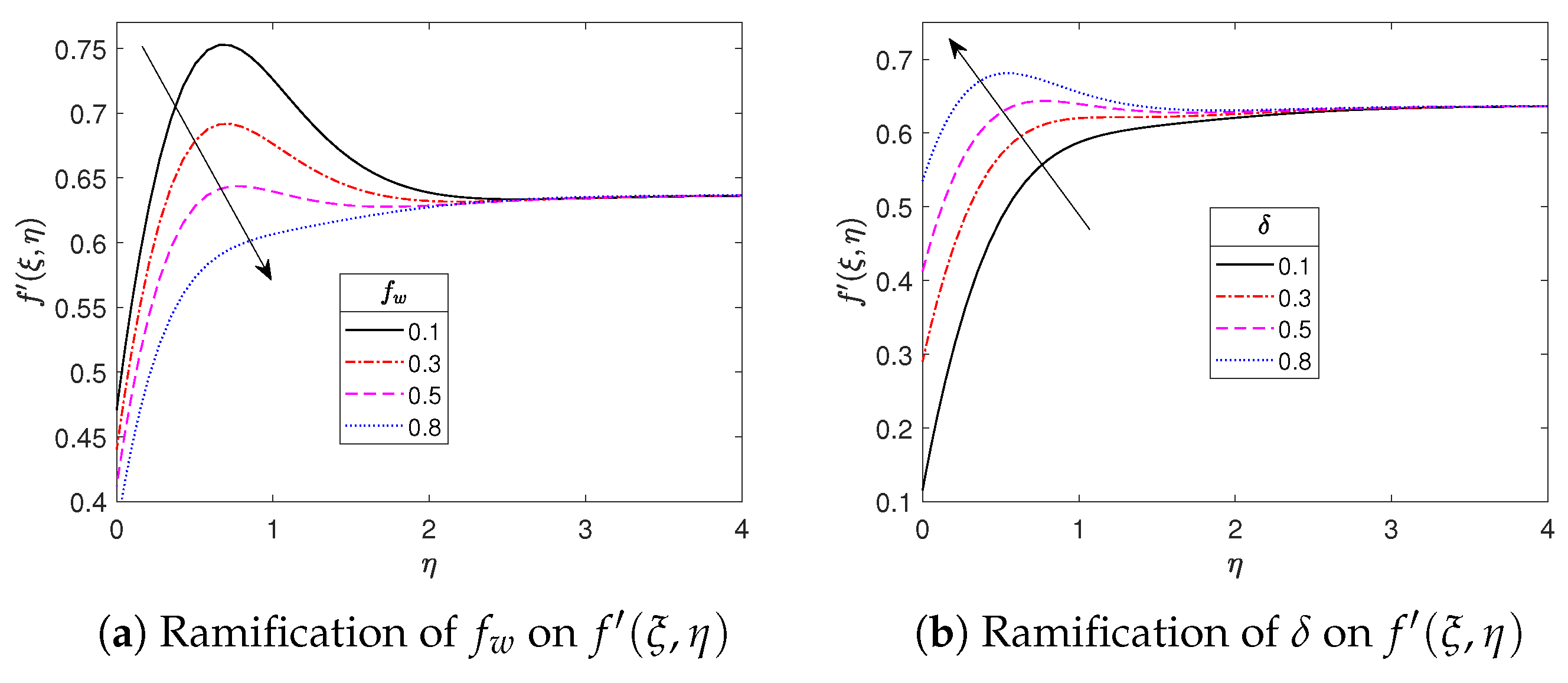
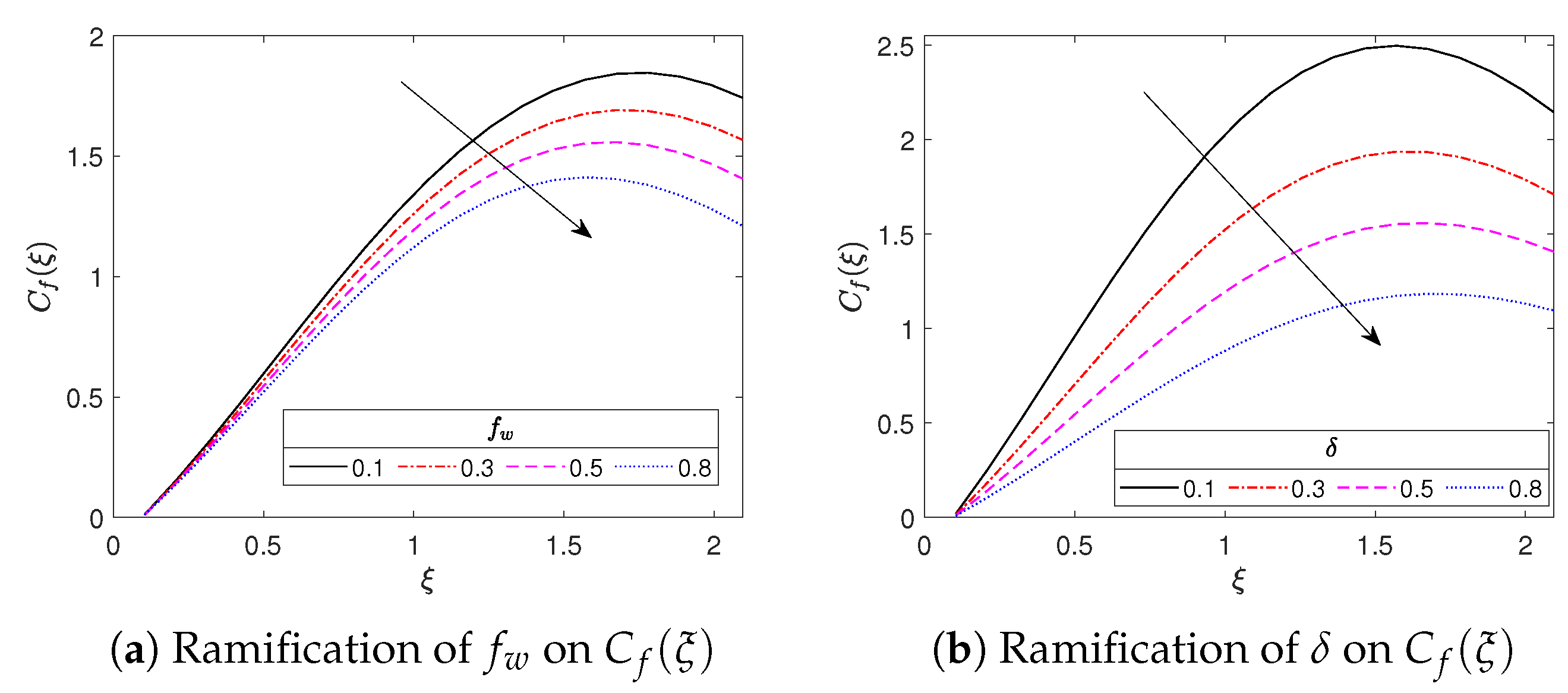
The consequence of the suction parameter $(f_w>0)$ and first-order velocity slip parameter $\left(\delta \right)$ on the velocity dissemination is portrayed in Figure 7. Figure 7a demonstrates that the velocity boundary layer’s thickness is diminished with the mounting values of the suction parameter. This deportment is owed to the fact that suction upshot plays a fundamental role in the removal of the fluid from the flow system; thus, momentum boundary layer thickness is remarkably decelerated. Figure 7b shows that dimensionless velocity is maximized with the growing velocity slip variable. This is on account of the acceleration in the fluid flow and the corresponding momentum boundary layer thickness as the velocity slip effect is increased. The acceleration of the fluid velocity component with improved velocity slip impact was also disclosed by Gaffar et al. [6] and Prasad et al. [45] in the absence of microbes.

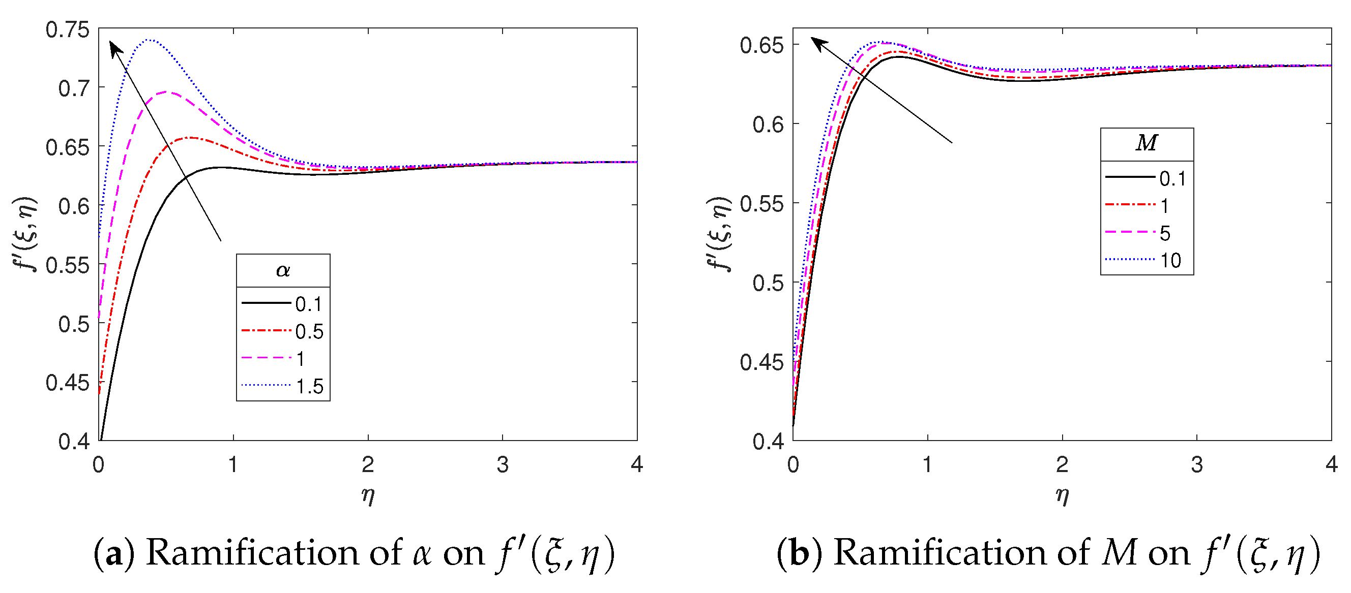
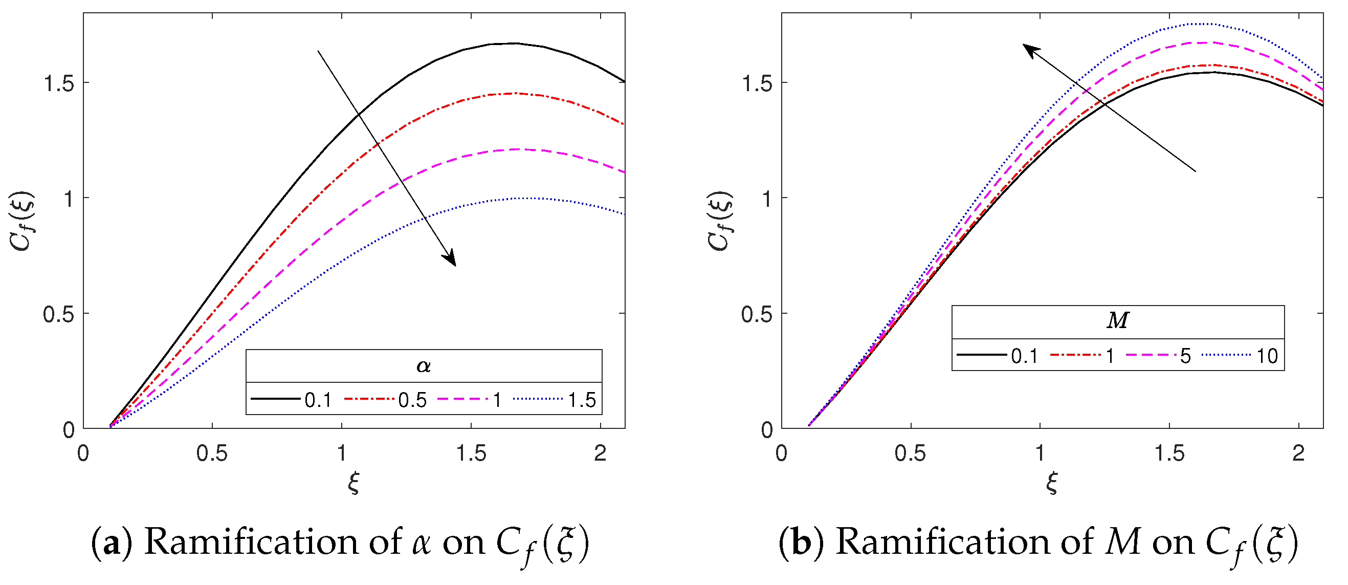
The variation of dimensionless velocity against the transverse coordinate $\left(\eta \right)$ when the variable viscosity parameter $\left(\alpha \right)$ and the applied magnetic field parameter $\left(M\right)$ are varied is illustrated in Figure 8. It is clear that the velocity field is improved with rising values of the variable viscosity parameter (see Figure 8a). Physically, increasing values of $\alpha$ tend to augment the temperature variation $(T_f-T_{\infty }),$ consequently, the Williamson fluid bond is weakened and the intensity of the dynamic viscosity of the non-Newtonian material is minimized. As a result, the momentum boundary layer thickness is improved, and the fluid velocity is also accelerated. On the other hand, the dimensionless velocity of our nonlinear mixed convective flow is seen to be increased with mounting values of applied magnetic field parameter. This behaviour is opposite to that of the free convective flows (see Gaffar et al. [6]), where the velocity is declined by rising values of $M.$ From a physics perspective, in an electrically conducting fluid, the magnetic field operating in a transverse direction to the geometry generates a resistive force known as the Lorentz force. The resulting Lorentz force inhibits the velocity of the fluid, as is evident in the free convective flows. In the present problem, it is noteworthy that the velocity component portrays the mounting behaviour because of the existence of nonlinear mixed convection. The similar behaviour is adequately explained by Basha et al. [17] in the absence of gyrotactic microorganisms.

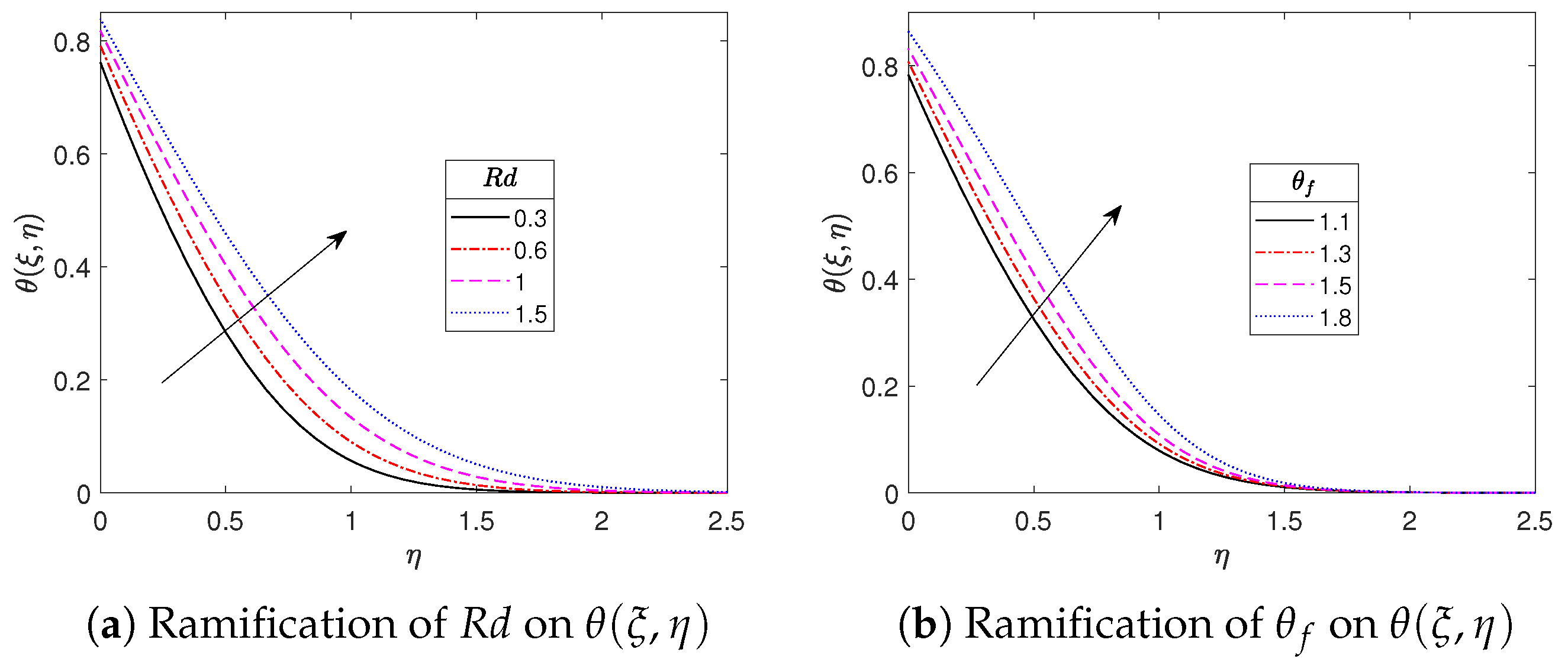
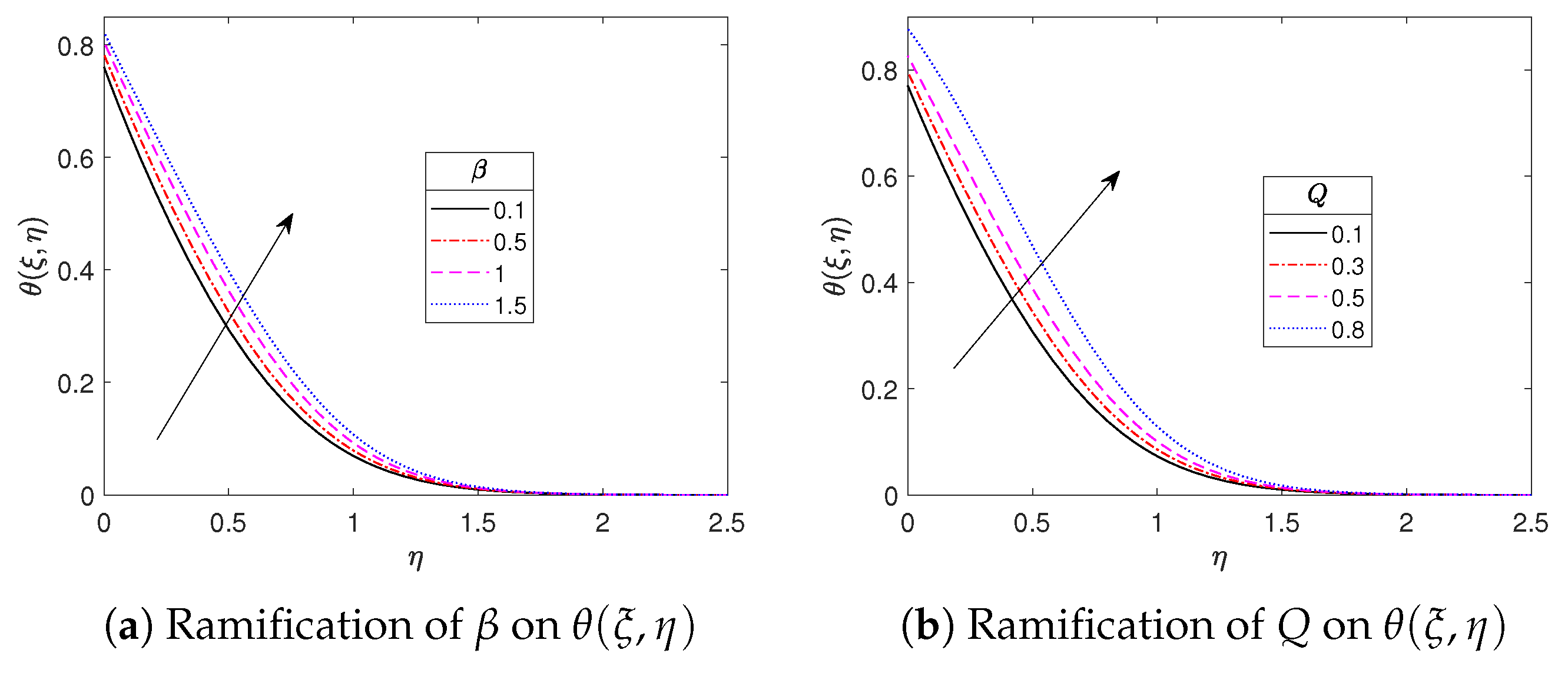
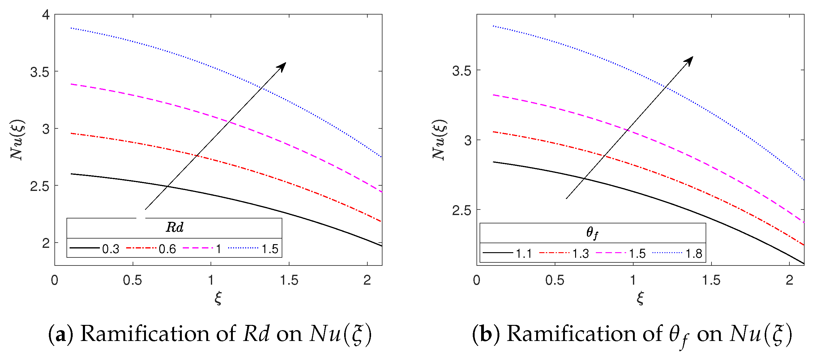
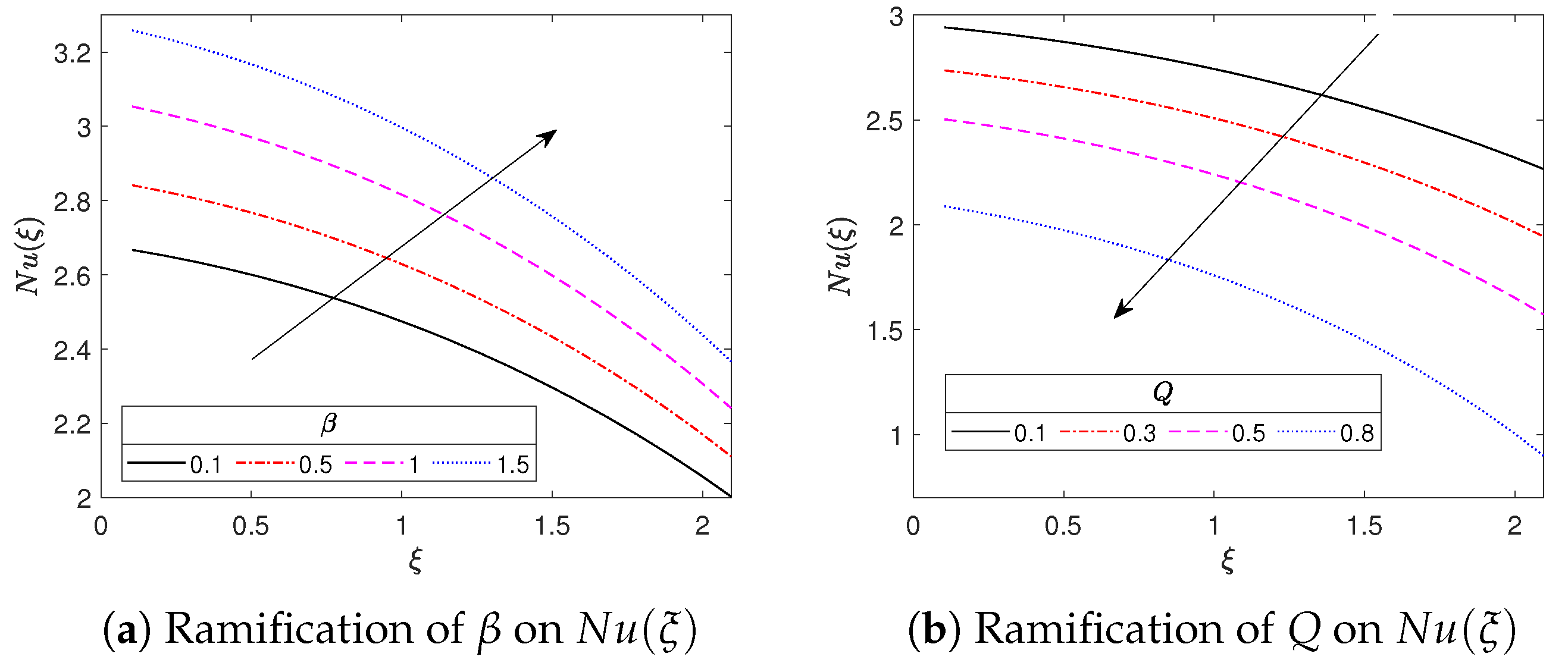
Figure 9 presents the effect of the thermal radiation parameter $\left(Rd\right)$ and surface temperature excess ratio $\left({\theta }_f\right)$ on the dimensionless temperature curves. From the first figure, it is noted that the temperature curve is enhanced by rising values of the thermal radiation parameter. This is because increments in thermal radiation energize the boundary layer and upsurge the heat radiation energy; consequently, both the fluid temperature and thermal boundary layer width are also improved. The Rosseland radiation absorption is enhanced by the rising values of the heat radiation parameter $Rd$; thus, radiative heat transmission rate to the fluid is upsurged, leading to an improvement in the temperature dispersion. On the other hand, the non-dimensional temperature is also increased by the escalating values of the temperature ratio parameter since the parameter ${\theta }_f$ improves the fluid’s thermal state. From a physics point of view, the greater values of the surface temperature excess ratio imply an upsurge in the temperature difference $(T_f-T_{\infty }),$ consequently, the temperature of the fluid is elevated. Figure 10 illustrates the ramifications of the variable thermal conductance parameter $\left(\beta \right)$ and heat generation parameter $(Q>0)$ on the temperature curves. Figure 10a reveals that the temperature curve improves with the escalation in $\beta ,$ which is owed to the excess amount of heat transmitted from the surface of the cylinder to the fluid. The parameter $\beta$ is directly proportional to the temperature difference. As a result, an elevation in the variable thermal conductance parameter causes a remarkable potential for thermal energy to convey more heat energy to the NPs, instigating a rise in the fluid temperature. Figure 10b shows that temperature distribution mounts with the rising values of the heat source parameter. It is worth pointing out that $Q>0$ represents the amount of heat produced within the system during the fluid flow. Thus, an increment in Q means that more heat is absorbed by the fluid, leading to an enhancement in the thermal boundary layer’s thickness and fluid temperature.

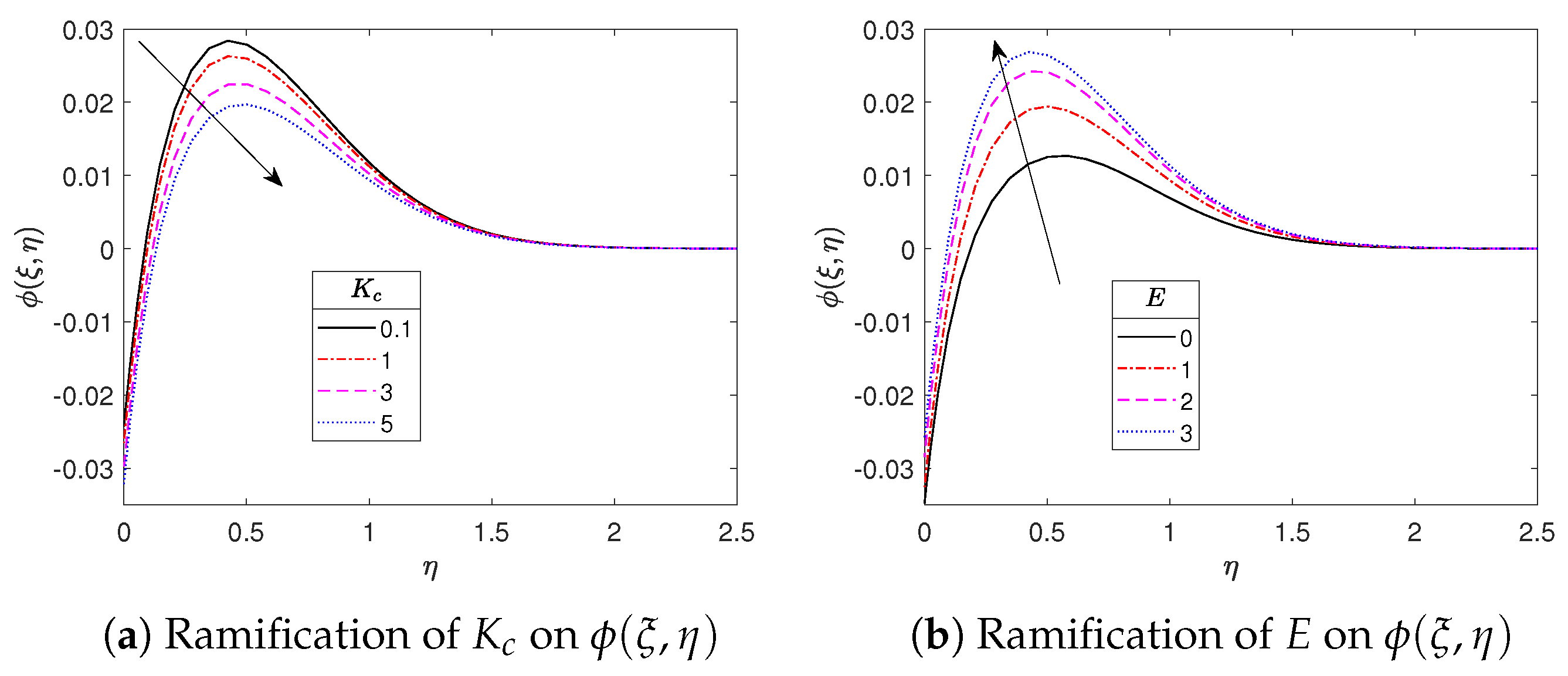
Figure 11 reveals the impact of the non-dimensional AE parameter $\left(E\right)$ and chemical reaction rate parameter $\left(K_c\right)$ on the non-dimensional NP species concentration distributions. From Figure 11a, it is clear that increasing the non-dimensional chemical reaction rate lessens the thickness of the non-dimensional concentration dissemination. The thinning in the non-dimensional species concentration dissemination is continuously occurring in conjunction with an enlarged non-dimensional concentration gradient. On the other hand, the rise in the non-dimensional AE impact decreases the non-dimensional wall concentration gradient. The physical justification for such a behaviour is that high AE slows down the chemical reaction process. As a result, both the non-dimensional species concentration profiles (see Figure 11b) and the thickness of the concentration boundary layer improve, leading to a reduction in the non-dimensional wall concentration gradient.

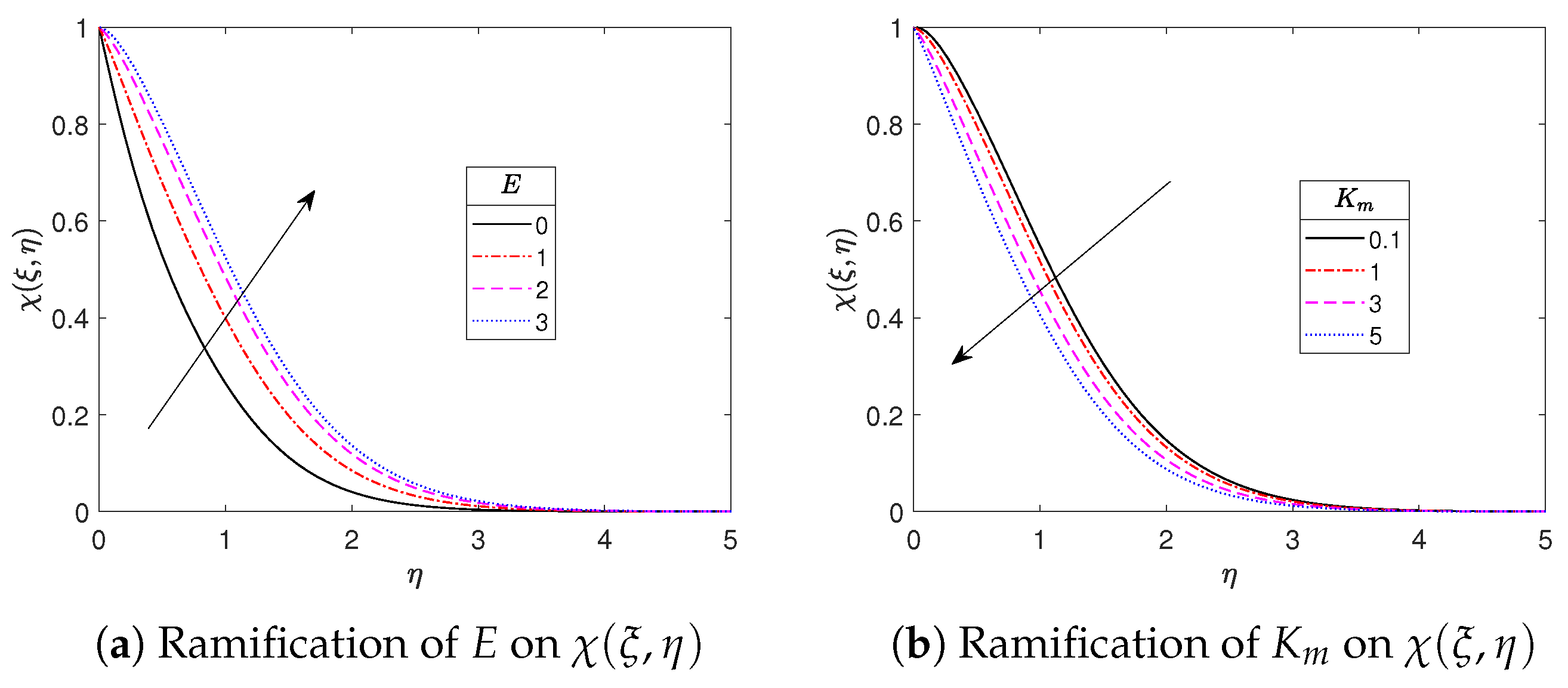
The impact of the AE parameter $\left(E\right)$ and microbial reaction rate parameter $\left(K_m\right)$ on the non-dimensional density of the motile microbes is portrayed in Figure 12. It is perceived from Figure 12a that the density of the motile microbes is reinforced by the rising values of the AE parameter. Since the microbial reaction process is improved by using AE, the motile microbe concentration profile is augmented to a greater extent. On the other hand, Figure 12b illustrates that the density of motile microbes declines with the augmenting values of the microbial reaction rate parameter. With an elevation in $K_m,$ the microorganisms’ diffusivity shrinks, for which less motile microorganism transfer occurs. In this phenomenon, the concentration of motile microorganisms drops as the values of $K_m$ increase.

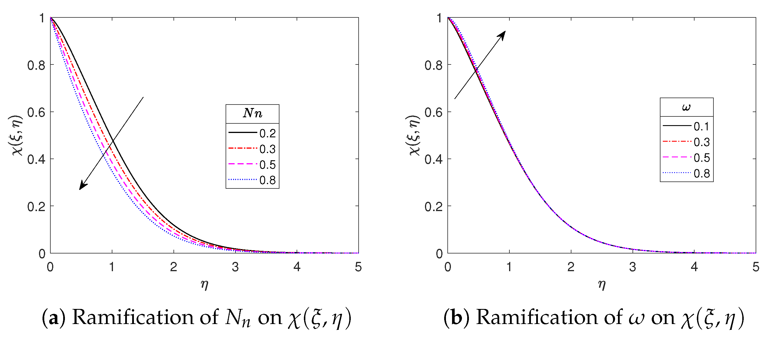
Figure 13 reveals the non-dimensional microorganism concentration dissemination for the different values of the motile microbe parameter $\left(\omega \right)$ and microbial Brownian motion parameter $\left(Nn\right)$. It is worth pointing out that the microbial Brownian motion is implied by the unrestricted mobility and unpredictable behaviour of motile microbes. The decline in the gyrotactic microorganism concentration profile for high $Nn$ indicates fewer motile microbes for the reaction (see Figure 13a). From a physics point of view, when $Nn$ gets larger, the random collision between motile microbes increases, which leads to a reduction in motile microorganism transfers. As a result, an elevation in $Nn$ resembles a decrement in the motile microbe concentration characteristics. In the other figure, there is an enhancement in the magnitude of motile microbes, in particular near the wall of the cylinder, when the bioconvection constant is raised. From formula $\omega =\frac{n_{\infty }}{n_w-n_{\infty }},$ we note that the motile microbe constant correlates the ambient density of the motile microbes to the density difference across the boundary layer. When $\omega$ upsurges, there is a larger density gradient across the boundary layer regime, which promotes the propulsion of motile microbes from the surface to the bulk flow. This results in an enhancement in the density of the motile microbes, in particular near the wall of the cylinder.

The ramification of the Williamson fluid parameter $\left(\mathsf{\Lambda }\right)$ and nonlinear thermal convection coefficient $\left(\mathsf{\Omega }\right)$ on the wall friction factor is disclosed in Figure 14. Figure 14a demonstrates that the surface drag coefficient is a decreasing function of the changing Williamson fluid parameter. Larger values of $\mathsf{\Lambda }$ imply that a long relaxation time is needed to yield excess fluid movement resistance, thus increasing the skin friction factor. Figure 14b shows that wall shear stress is also improved with a rise in the nonlinear temperature parameter since an upsurge in $\mathsf{\Omega }$ raises the density of the fluid flow, which in turn augments resistance to the flow. Figure 15 illustrates the upshots of the suction parameter $(f_w>0)$ and velocity slip parameter $\left(\delta \right)$ on the surface drag coefficient. It is perceived from Figure 15a that a greater suction parameter leads to a decrement in the skin friction factor. This demonstrates that an improvement in the cylinder surface’s porosity causes an increment in the fluid flow resistance. In the other figure, surface shear stress is also diminished by increasing the values of $\delta$, since the fluid flow is decelerated along the cylinder when $\delta$ is raised. As noted in Prasad et al. [45], there is progressive movement in the peak shear stress locations far away from the lower stagnation when $\delta$ is elevated. Thus, the repercussion of the wall slip is noted to be significant on the boundary layer features of the Williamson fluid flow from the horizontal cylinder.

Figure 16 highlights the consequences of the variable viscosity parameter $\left(\alpha \right)$ and applied magnetic field parameter $\left(M\right)$ on the wall friction factor. From the first figure, it is clear that the skin friction factor is reduced by the rise in $\alpha$ because of a lower resistance to flow on the cylinder surface. When there is less resistance to flow, the fluid moves more freely along the surface, causing a reduction in the shear stress and skin friction coefficient. On the other hand, a rise in the magnetic field parameter augments the surface drag coefficient. This is because the Lorentz force monitors the rate at which the fluid particles tend to move; thus, the drag coefficient increases at the level of the cylinder’s surface.

The upshots of the heat radiation parameter $\left(Rd\right)$ and temperature ratio parameter $\left({\theta }_f\right)$ on the dimensionless Nusselt number are depicted in Figure 17. From Figure 17a, it is clear that the elevation in $Rd$ suggests a prominent increment in the local Nusselt number. This deportment is in harmony with the fact that heat transportation becomes superior with the radiation effect. Figure 17b illustrates that the heat transfer rate escalates with increment in the surface temperature excess ratio since the presence of the temperature ratio parameter ${\theta }_f=\frac{T_f}{T_{\infty }}$ contributes towards enhancement of the temperature of the fluid.

Figure 18 illustrates the distribution of the local Nusselt number for various variable thermal conductance $\left(\beta \right)$ and heat generation parameters $(Q>0)$. The local Nusselt number is enhanced by rising values of $\beta$ as seen in Figure 18a. This behaviour is due to the fact that the cylinder distributes additional heat by intensifying $\beta ,$ which in turn accelerate the heat distribution in the system as well as the rate of heat transport. Figure 18b demonstrates that escalation in Q gives rise to higher Nusselt numbers. This is because the mechanisms of heat source produce a layer of warmed fluid near the cylindrical surface; thus, the temperature of the fluid surpasses the temperature of the cylinder’s surface.

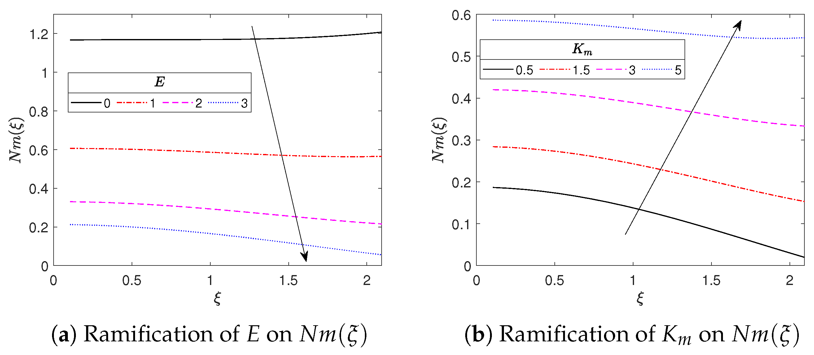
The variation in the dimensionless local density number of the motile microbes with the AE parameter $\left(E\right)$ and microbial reaction parameter $\left(K_m\right)$ is depicted in Figure 19. It is evident that the density number of motile microbes drops when the dimensionless AE parameter is increased. This signifies that as the Reynolds number escalates, the diffusion rate prevails over the motile microbe transfer rate. The lower the density number of motile microbes, the more AE there is. Higher AE implies that more energy is needed for the motile microbes to have a fruitful collision. On the other hand, the density number of motile microorganisms is noted to be remarkably enhanced by strong motile microbial reactions. 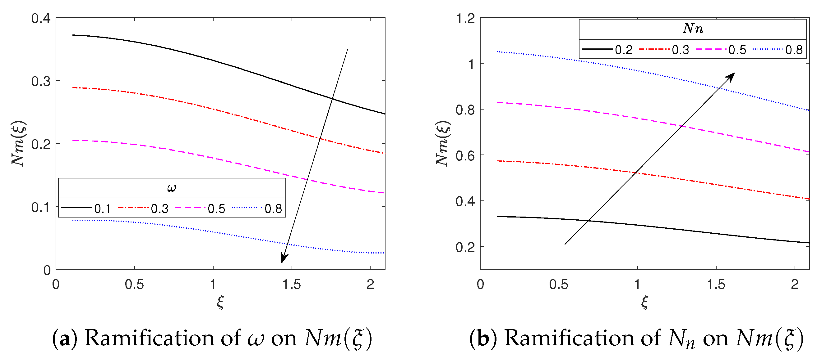Figure 20 elucidates the impact of the bioconvection constant $\left(\omega \right)$ and microbial Brownian motion parameter $\left(Nn\right)$ on the density number of motile microbes. Figure 20a reveals that as $Nn$ augments, the density number of motile microbes is enhanced. This might be attributed to the fact that motile microbes in the Williamson fluid are moving haphazardly. The other figure demonstrates that the motile microbe transfer rate is reduced with the growing values of the motile microbes parameter.

5. Concluding Remarks

A mathematical model has been described for the bioconvective flow of magneto-Williamson NF comprising motile microbes through a radiative horizontal circular cylinder in a porous medium with nonlinear Boussinesq approximation, heat generation/assimilation, variable fluid properties, AE, chemical and microbial reactions, and Brownian motion for both NPs and motile microorganisms. The modified Buongiorno NF model is employed, and the problem is modeled subject to velocity slip, suction/injection, and heat-convective and zero mass flux boundary conditions. Using appropriate similarity transformations, a non-dimensional partial differential boundary value problem has been derived for the transport features. The resulting coupled partial differential equation system has been solved numerically with appropriate boundary conditions at the wall and in the free stream, using an overlapping grid-based SCM that employs the local linearisation technique to deal with non-linearity in the flow problem. The findings confirmed that the overlapping grid-based numerical scheme should be the most preferred numerical method for solving flow problems similar to the one considered in the current work. The remaining prominent numerical results of the present investigation are recapitulated as follows:

• Nonlinear thermal convection, velocity slip, magnetic field, and variable viscosity parameters accelerate NF motion, while the Williamson fluid and suction parameters decelerate the fluid flow.
• The surface drag coefficient is lifted for the Williamson fluid, nonlinear convection, and magnetic field parameters, but decays for suction, velocity slip, and variable viscosity.
• The NF temperature and heat relocation rate are enhanced by rising thermal radiation, temperature ratio, and fluctuating thermal conductivity parameters.
• The inclusion of AE assists in raising concentrations of NPs and motile microbes.
• The incorporation of microbial reactions and Brownian motion contributes to a rise in motile microbes transfer rate and a reduction in the density of motile microbes.

In the near future, the current problem can be extended to the bioconvection flow of other non-Newtonian fluid models by considering the Tiwari–Das nanofluid model with other features such as electro-magnetohydrodynamics, viscous dissipation, Joule heating, and microbial growth. To optimize thermal processes, analysis of entropy generation will also be studied.