Microstructure and Inertial Characteristics of MHD Suspended SWCNTs and MWCNTs Based Maxwell Nanofluid Flow with Bio-Convection and Entropy Generation Past a Permeable Vertical Cone

Abstract

In this research work, our goal is to scrutinize the case, where water-based nanofluids having single-wall and multi-wall carbon nanotubes (CNTs) flow through a vertical cone. The second law of thermodynamic is taken for the aim of scheming effective heat storage units. The body package is layered in convective heat and diluted permeable medium. The effects of Joule heating, rotary microorganisms, heat generation/absorption, chemical reactions, and heat radiation increase the novelty of the established model. By using a local similarity transformation technique, the partial differential equations (PDEs) change into a coupled differential equation. By using the numerical technique, bvp4c, to get the solution of the conservation equations and their relevant boundary conditions. The parameters appearing in the distribution analysis of the alliance are scrutinized in detail, and the consequences are depicted graphically. It can be perceived that in the situation of composed nanotubes, the velocity of fluid decreases as the magnetic field is increased.

1. Introduction

In the present era, nanofluid is getting importance from the researchers due to its diverse application in the industrial field. For instance, they are available in polymer manufacturing, gas turbines, power generators, glass fabric, paper production, wire drawing, and many more. Nanofluid is a sort of heat transport medium containing nanoparticles under 100 nm, which are reliably and consistently scattered in a base fluid like water, oil, and ethylene glycol. These scattered nanoparticles, for the most part, a metal or metal oxide massively improve the thermal conductivity of the nanofluid, upgrades conduction, and convection coefficients, mulling over more heat transport. Enhancing the thermal specifications of liquids leads to a greater level of connective flow in thermal units. For heat transfer enhancement, adding additives to the operant liquids for modifying their thermal features are very attractive method. For this, a way has been represented by enhancement in nanotechnology. The meaning of ‘nanofluid‘ has been expressed by Choi [1] in 1995 for increasing heat transfer specifications of convectional fluids. A total report on the productivity of temperature transformation in the sunlight-based authority with the nanoliquid was done by Chen et al. [2]. They originate that the presentation of photo thermal change in the gatherer expanded by 96.93% and 52% at 30 and 75 °C separately, an entirely reasonable liquid for sun powered authorities which have the shortest fascination in low-temperatures. Oudina [3,4] examined nanomaterial conduct esoteric an annulus with different designs of temperature foundations. They used an arithmetical methodology and introduced soundness investigation. Mesoscopic line for investigating nanomaterial course through permeable area was introduced by Sheikholeslami [5]. They utilized Lorentz force to switch the stream style inside an opening. Chougule et al. [6] initiate that because of the low association of nano-powders, a pressure drop is critical in the curved cylinder when they utilized carbon nanotubes (CNTs) instead of unadulterated water. Besides, a curved cylinder with loop supplements improves better Nusselt number as a result of the rate of energy altercation increment because of this reality nano-powders have arbitrary and unpredictable movement in the liquids. Numerically, the plan assessment of a whirling stream microchannel for incredible warmth transition uses had been examined by Hartmann-Priesnitz et al. [7] who displayed the operant liquids as Cu-H₂O nanomaterial in the laminar stream. Ding et al. [8] portrayed nanofluids that depend on CNTs, which depend upon the heat of the base liquid, and set up that when the liquid heat is 25 °C, the warm conductivity can be expanded by up to 30%, but can be increased by 79% observed at 40 °C. Pop and Watanabe [9] carried out a theoretical analysis with the main aim to discuss the influence of injection/suction on fluid flowing over a cone with free convection and heat flux. The authors used different differential methods to solve the existing equation describing the flow. Xu [10] recently studied time-dependent hybrid nanofluid with mixed convection in rotating disks multiple kinds of nanoparticles are taken here. A numerical approach is used for the solution. Flaccid devices are used by investigators in an earlier investigation to improve the convective coefficient [11]. Many researchers used a combination of both concepts to enhance convective coefficient by use of insert with nanofluids. Heat transfer and friction element characteristics on warped tape with Al₂O₃/water nanofluid are analyzed by Sharma et al. [12]. Zhang [13] has investigated adapted computational approaches in which a 2-D effective heat capacity model is used for forecasting the fleeting heat transmission procedure of the building envelopes equipped with phase change materials (PCM). The deviations against test data made by the principal procedures were viewed as especially bigger than the changed methodologies adjusted techniques. Sun et al. [14] have experimentally deliberated the heat transmission rate augmentation produced by natural convection of PCMs experiencing melting. The thermophysical properties of nanofluids have been discussed by Phuoc et al. [15]. The increase in the transfer of heat of SWCNTs-glycol-based nanofluids was examined by Harish et al. [16]. It was found that while 0.2% by volume of SNTs was added to ethylene glycol, the thermal conductivity increased by 14.8%. The magnetohydrodynamic (MHD) 3-D Maxwell nanofluid boundary layer flow with convective boundary conditions on a biaxially stretched sheet was explored by Hayat et al. [17].

Nowadays the main concerns of scientists are to make the strategies that control the ingesting of skilled vitality. In the field of thermal structuring, the key objective is to achieve the best viability of contraptions and with the base loss of warmth, scouring, and spread during the mechanical procedures. All the heat gadgets take a shot at the guideline of thermodynamics and produce. Thermodynamic second laws used to look at the irreversibility in terms of the entropy age rate. Entropy growth is abused to elucidate the exhibition of various settings in present-day and structure solicitations. Entropy is imitative from the Greek word Entropia, which suggests “moving toward” or “alteration”. Entropy figuring is basic as it orders the factors for energy forfeiture. Bejan [18] offered the clue of an entropy generation problem. Ellahi et al. [19] studied the influence of entropy optimization on natural convective nanoliquid stream. A multiple turbulator has been engaged by Sheikholeslami et al. [20] to enlarge the involvement of nanomaterial inside a tube. They verified that thermal irreversibility improves with the upsurge of subordinate flow. The related research work in a similar filed can be seen in [21,22].

The attractive properties of carbon nanotubes (CNTs) include mechanical and chemical stability, excellent thermal and electrical conductivity, lightweight and physicochemical reliability, making them a desirable material in the manufacture of electrochemical devices. Considering this exciting feature of carbon nanotubes, in this research work, our goal was to scrutinize the case where water-based nanofluids having single-wall and multi-wall CNTs flow through a vertical cone. The body package is layered in convective heat and diluted permeable medium. The effects of Joule heating, rotary microorganisms, and heat generation/absorption, chemical reactions, and heat radiation increase the novelty of the established model. By using a local similarity transformation technique, the PDE is changed into a coupled differential equation. By using the Homotopy analysis method to get the solution of the conservation equations and their relevant Boundary conditions. The parameters appearing in the distribution analysis of the alliance are scrutinized, and the consequences are depicted graphically. It can be perceived that on account of the two nanotubes, the velocity of fluid decreases as the magnetic is increased. Moreover, the thickness of moving microorganisms is decreased compared to more estimation of biological convection constants.

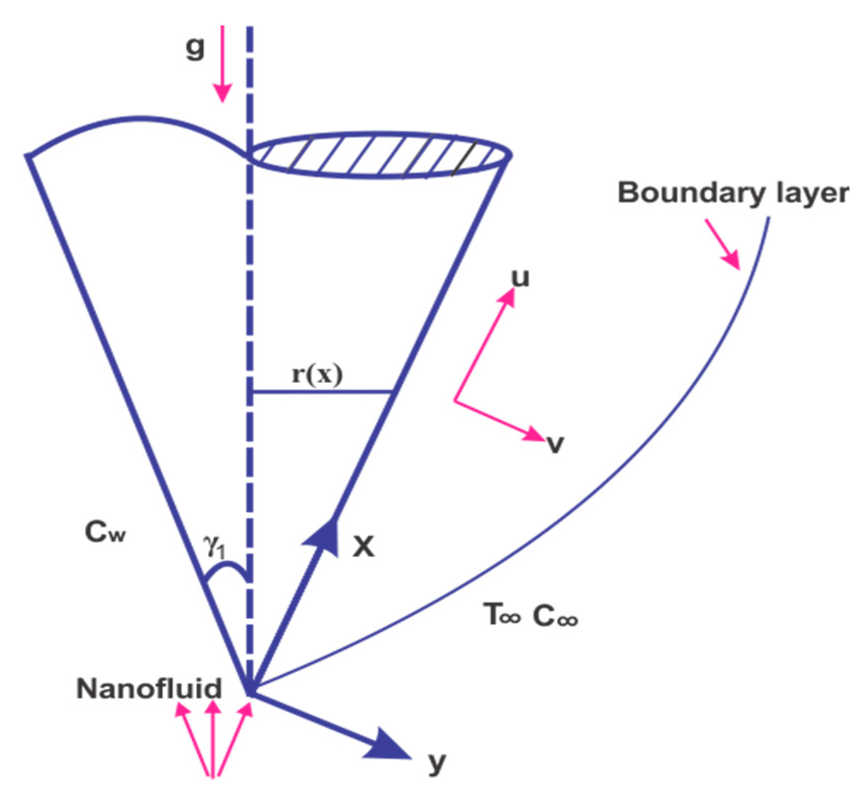
2. Mathematical Analysis

We suppose the flow of magnetohydrodynamic (MHD) mixed convective viscous water-based micropolar nanofluidic of CNTs on a vertical cone in a penetrable medium. The coordinate system for the flow phenomena is chosen is such a way that x-coordinate is parallel with the direction of the fluid. Energy expression with thermal radiation dissipation, thermal flux, and Joule heating is measured. Irreversibility investigation with chemical reaction is investigated. Entropy rate is determined. Slip impact is likewise talked about. A magnetic field of constant strength β₀ is applied vertically. The temperature (T) and concentration ponder (C). Speeding up because gravity acts downwards. Problem geometry is featured in Figure 1.

From the above suppositions, the resulting modeled equations are:

$${\left(ru\right)}_x+{\left(rv\right)}_y=0$$

(1)

$$\begin{array}{l}u{u}_x+v{u}_x+\lambda \left(u^2{u}_{xx}+v^2{u}_{yy}+2uv{u}_{xy}\right)=\frac{{\mathsf{\mu }}_{nf}}{{\mathsf{\rho }}_{nf}}{u}_{yy}-\frac{{\mathsf{\mu }}_{nf}}{{\mathsf{\rho }}_{nf}}\frac{u}{K}+\\ g\left[\mathsf{\beta }\left(T-T_{\infty }\right)-\mathsf{\beta }*\left(C-C_{\infty }\right)-\mathsf{\beta }*\gamma \left(n-n_{\infty }\right)\right]\cos {\gamma }_1-\frac{{\mathsf{\sigma }}_{nf}{\mathsf{\beta }}_0^2}{{\mathsf{\rho }}_{nf}}u+K{N}_y\end{array}$$

(2)

$$u{T}_x+v{T}_y={\mathsf{\alpha }}_{nf}{T}_{yy}-\frac{1}{{\left({\mathsf{\rho }}_{cp}\right)}_{nf}}{\left(q_r\right)}_y+\frac{Q_0}{{\left({\mathsf{\rho }}_{cp}\right)}_{nf}}\left(T-T_{\infty }\right)+\frac{\mathsf{\sigma }{\mathsf{\beta }}_0^2}{{\left({\mathsf{\rho }}_{cp}\right)}_{nf}}{u}^2$$

(3)

$$u{N}_x+v{N}_y=\frac{{\gamma }_{nf}^{*}}{{\mathsf{\rho }}_{nf}}{N}_{yy}-\frac{k}{{\mathsf{\rho }}_{nf}}\left(2N+u_y\right)$$

(4)

$$u{C}_x+v{C}_y=D_m{C}_{yy}-k_r\left(C-C_{\infty }\right)$$

(5)

$$u{n}_x+v{n}_y+\frac{bW}{\left(C_w-C_0\right)}{\left(n{C}_y\right)}_y=D_n{n}_{yy}$$

(6)

with the corresponding boundary conditions

$$\begin{array}{l}u=0 ,v=V_1, N=0,T_y=\frac{h_f\left(T_f-T\right)}{-k_{nf}}, C_w=C=dx+C_0,n=n_w, At y=a\\ u\to 0,N\to 0,C\to C_{\infty }=C_0+ex,T\to T_{\infty },n\to n_w At y\to \infty \end{array}$$

(7)

where, (β, β*), (μ_nf, μ_f), (ρ_CHT, ρ_f), β₀, α_nf, V₀, h_f, (d, e), Q₀, ((ρ_cp)_f, (ρ_cp)_nf), (k_f, k_nf, k), D_n, k_r, W_c, D_m, q_r, γ₁ indicate coefficients of thermal and solutal expansion, dynamic viscosities, densities, magnetic strength, thermal modified diffusivity, suction/injection parameter, convective parameter, dimensionless constants of concentration, heat generation/absorption parameter, heat capacities, thermal conductivity, diffusivity of microorganisms, chemical reaction rate, coefficient, extreme cell swimming motion, Brownian diffusion, radiation coefficient, and cone half-angle, respectively. In Equation (7) the term V₁ characterizes the mass transmission and defined as $V_1=-\left(\frac{3}{4}a{x}^{-1}R{\left(a_x\right)}^{\frac{1}{4}}\right)V_0$. In case of V₁ < 0, the mass transfer is for injection and V₁ > 0 shows suction.

$$\begin{array}{l}{\mathsf{\alpha }}_{nf}=\frac{k_{nf}}{{\mathsf{\rho }}_{nf}{\left(c_p\right)}_{nf}},\frac{k_{nf}}{k_f}=\frac{\left(1-\mathsf{\varphi }\right)+2\mathsf{\varphi }\frac{k_{CNT}}{k_{CNT}-k_f}\ell n\left(\frac{k_{CNT}+k_f}{2k_f}\right)}{\left(1-\mathsf{\varphi }\right)+2\mathsf{\varphi }\frac{k_{nf}}{k_{CNT}-k_f}\ell n\left(\frac{k_{CNT}+k_f}{2k_f}\right)}\\ {\nu }_{nf}=\frac{{\mathsf{\mu }}_{nf}}{{\mathsf{\rho }}_{nf}},{\gamma }_{nf}^{*}=\left({\mathsf{\mu }}_{nf}+0.5k\right)j,{\mathsf{\rho }}_{nf}=\left(1-\mathsf{\varphi }\right){\mathsf{\rho }}_f+\mathsf{\varphi }{\mathsf{\rho }}_{CNT},{\mathsf{\mu }}_{nf}=\mathsf{\mu }{\left(1-\mathsf{\varphi }\right)}^{-2.5}\\ \frac{{\mathsf{\sigma }}_{nf}}{{\mathsf{\sigma }}_f}=1-\frac{3\left(\frac{{\mathsf{\sigma }}_s}{{\mathsf{\sigma }}_f}-1\right)\mathsf{\varphi }}{\left(\frac{{\mathsf{\sigma }}_s}{{\mathsf{\sigma }}_f}-1\right)\mathsf{\varphi }-\left(\frac{{\mathsf{\sigma }}_s}{{\mathsf{\sigma }}_f}+2\right)}\end{array}$$

(8)

$$\begin{array}{l}\mathsf{\psi }=\mathsf{\alpha }R{a}_x^{1/4}f\left(\mathsf{\eta }\right),g\left(\mathsf{\eta }\right)=\frac{C-C_{\infty }}{C_w-C_0},\mathsf{\eta }=\frac{y}{x}R{a}_x^{1/4}\\ \mathsf{\theta }\left(\mathsf{\eta }\right)=\frac{T-T_{\infty }}{T_w-T_{\infty }},\mathrm{h}\left(\mathsf{\eta }\right)=\frac{n-n_{\infty }}{n_w-n_{\infty }},\mathrm{S}\left(\mathsf{\eta }\right)=\frac{{\mathsf{\rho }}_f{x}^{2}NR{a}_x^{-3/4}}{{\mathsf{\mu }}_f}\end{array}$$

(9)

Using Equations (8) and (9), Equation (1) is satisfied and Equations (2)–(6) are written as

$$\begin{array}{l}{f}^{‴}+-k_1{f}^{\prime }+{\left(1-\mathsf{\varphi }\right)}^{2.5}\left(1-\mathsf{\varphi }+\mathsf{\varphi }\frac{{\mathsf{\rho }}_{CNT}}{{\mathsf{\rho }}_f}\right)[\mathsf{\theta }-N_{r}g-R_{b}h]-{\left(1-\mathsf{\varphi }\right)}^{2.5}M{f}^{\prime }+\\ K{\left(1-\mathsf{\varphi }\right)}^{2.5}\left(1-\mathsf{\varphi }+\mathsf{\varphi }\frac{{\mathsf{\rho }}_{CNT}}{{\mathsf{\rho }}_f}\right)S^{\prime }+\frac{1}{2\mathrm{Pr}}{\left(1-\mathsf{\varphi }\right)}^{2.5}\left(1-\mathsf{\varphi }+\mathsf{\varphi }\frac{{\mathsf{\rho }}_{CNT}}{{\mathsf{\rho }}_f}\right)\\ \{{f^{\prime }}^2+\frac{1}{2}f{f}^{″}\}-\frac{\mathsf{\beta }}{4\mathrm{Pr}}{\left(1-\mathsf{\varphi }\right)}^{2.5}\left(1-\mathsf{\varphi }+\mathsf{\varphi }\frac{{\mathsf{\rho }}_{CNT}}{{\mathsf{\rho }}_f}\right)\left(3{f^{\prime }}^3+\frac{1}{4}{f}^{″}{f}^2-\frac{5}{2}{f}^{″}{f}^{\prime }f\right)=0\end{array}$$

(10)

$$\frac{k_{nf}}{k_f}\left(1+Rd\right){\mathsf{\theta }}^{″}+\frac{3}{4}\left(1-\mathsf{\varphi }+\mathsf{\varphi }\frac{{\mathsf{\rho }}_{CNT}}{{\mathsf{\rho }}_f}\right)f{\mathsf{\theta }}^{\prime }+\gamma \mathsf{\theta }+\mathrm{Pr}EcM{f^{\prime }}^2=0$$

(11)

$$S^{″}-\gamma *\left(2S+\mathsf{\alpha }{f}^{″}\right)+\frac{1}{4\mathrm{Pr}}\frac{{\left(1-\mathsf{\varphi }\right)}^{2.5}\left(1-\mathsf{\varphi }+\mathsf{\varphi }\frac{{\mathsf{\rho }}_{CNT}}{{\mathsf{\rho }}_f}\right)}{\left(1+0.5K\right)}\left(5S{f}^{\prime }+S^{\prime }f\right)=0$$

(12)

$$g^{″}+\frac{3}{4}Scf{g}^{\prime }-Scn{f}^{\prime }-G_{r}g=0$$

(13)

$$h^{″}+\frac{3}{4}{L}_{b}f{h}^{\prime }-P_e\left(h^{\prime }{g}^{\prime }+\left(h+\delta \right)g^{″}\right)=0$$

(14)

$$\begin{array}{l}{f}^{\prime }\left(0\right)=0,f\left(0\right)=V_0,\frac{k_{nf}}{k_f}{\mathsf{\theta }}^{\prime }\left(0\right)=-B_1\left(1-\mathsf{\theta }\left(0\right)\right),\mathrm{S}\left(0\right)=0,h\left(0\right)=1,g\left(0\right)=1-n,\\ f^{\prime }(\infty )\to 0,S(\infty )\to 0,\mathsf{\theta }(\infty )\to 0,h(\infty )\to 0,g(\infty )\to 0\end{array}$$

(15)

Non-dimensional form of parameters is specified and defined as below in Abbreviations.

3. Entropy Generation Modeling

To include the irreversibility sources, below equations can be used:

$$\begin{array}{l}{S^{‴}}_{gen}=\frac{k_{nf}}{k_f}\left(1+\frac{16T_{\infty }^3\mathsf{\sigma }*}{3k*k_{nf}}\right)\left(T_{yy}\right)+\frac{{\mathsf{\mu }}_{nf}}{T_{\infty }}{\left(u_y\right)}^2+\frac{\mathsf{\sigma }}{T_{\infty }}{\mathsf{\beta }}_0^2{u}^2+\frac{{\mathsf{\mu }}_{nf}}{T_{\infty }k}{u}^2+\\ \frac{RD}{C_{\infty }}{\left(C_y\right)}^2+\frac{RD}{T_{\infty }}\left(T_y\right)\left(C_y\right)\end{array}$$

(16)

where

$$N_G=\frac{{S^{‴}}_{gen}}{{S^{‴}}_0}$$

(17)

$\left({S^{‴}}_{gen}\right)$ is irreversibility optimization rate and $\left(S^{‴}\right)$ the characteristic irreversibility optimization rate signified by:

$$\begin{array}{l}{N}_G=\frac{k_{nf}}{k_f}\left(1+R\right)R{a}_x{{\mathsf{\theta }}^{\prime }}^2+\frac{1}{{\left(1-\mathsf{\varphi }\right)}^{2.5}}\frac{BrR{a}_x}{\mathsf{\alpha }}\left({f^{″}}^2+k_1{f^{\prime }}^2\right)+\\ \frac{BrR{a}_{x}M}{\mathsf{\alpha }}{f^{\prime }}^2+\lambda \left(\frac{\mathsf{\xi }}{\mathsf{\alpha }}\right)R{a}_x{g^{\prime }}^2 +\frac{\mathsf{\xi }}{\mathsf{\alpha }}R{a}_x\lambda {\mathsf{\theta }}^{\prime }{g}^{\prime }\end{array}$$

(18)

where $Br\left(=\frac{{\mathsf{\mu }}_f{U}_w}{k_f\Delta T}\right)$ Brinkman number, $\mathsf{\alpha }\left(=\frac{\Delta T}{T_{\infty }}\right)$ diffusion parameter, $\mathsf{\xi }\left(=\frac{\Delta C}{C_{\infty }}\right)$ concentration ratio parameter, and $\lambda \left(=\frac{RD{C}_{\infty }}{k_f}\right)$ temperature difference parameter, respectively.

4. Engineering Quantities

4.1. Skin Friction Coefficients C_Fx

Mathematically, it is defined as

$$C_{Fx}=\frac{2{\mathsf{\phi }}_w}{\mathsf{\rho }{u}_{\infty }^2}$$

(19)

The dimensionless form is

$${\mathrm{Re}}_x^{1/2}{C}_{Fx}=\left(1+K\right)\frac{1}{{\left(1-\mathsf{\varphi }\right)}^{2.5}}{f}^{″}\left(0\right)$$

(20)

In which ${\mathrm{Re}}_x^{1/2}$ designates Reynold number.

4.2. Heat Transfer Rate

$N{u}_x$ is

$$N{u}_x=\frac{x{Q}_w}{k({\mathrm{T}}_w-{\mathrm{T}}_{\infty })}$$

(21)

where the heat flux $Q_w$ is

$${Q_w=-\frac{k_{nf}}{\mathsf{\kappa }}\left(\frac{4{\mathsf{\sigma }}_e}{3\mathsf{\kappa }{\mathsf{\kappa }}_R}{\mathrm{T}}_{\infty }{}^3+1\right){\mathrm{T}}_y|}_{y=0}$$

(22)

$${\mathrm{Re}}_x^{-1/2}N{u}_x=-\frac{k_{nf}}{k_f}\left(1+Rd\right){\mathsf{\theta }}^{\prime }\left(0\right)$$

(23)

4.3. Mass Transfer Rate

Sherwood number $S{h}_x$ is defined as

$$S_h{}_x=\frac{x{h}_w}{D_B\left(C_w-C_{\infty }\right)}$$

(24)

$${h_w=-D_B{C}_y|}_{y=0}$$

(25)

$${\mathrm{Re}}_x^{-1/2}S{h}_x=-g^{\prime }\left(0\right)$$

(26)

4.4. Local Density of Motile Microorganisms

Sherwood number $N_{nx}$ are stated as

$$N_{nx}=\frac{x{Q}_n}{D_n\left(n_w-n_{\infty }\right)}$$

(27)

$${Q_n=-D_n{n}_y|}_{y=0}$$

(28)

After simplification

$${\mathrm{Re}}_x^{-1/2}{\rm N}{n}_x=-h^{\prime }\left(0\right)$$

(29)

5. Solution Technique

In this present work, the constitutive equations for the given problem are mathematically modeled under the following assumptions, heat generation/absorption, permeable medium, the geometry is taken to be a vertical cone, SWCNTs-water, and MWCNTs-water, convective boundary circumstances. The highly non-linear ODEs were obtained from PDEs by using the transformation technique. Hence, we employed a numerical system on the highly non-linear transformed differential equations.

Equations (12)–(16), along with boundary value problem (17) and (18), called a bvp4c just a name built-in Matlab function which is based on finite difference method and found the solutions computationally which is captured both in tables. Equations (1)–(6) and as well as in graphs. For this purpose, we can transform our differential equations into an arrangement of first order differential equations by letting the new factors

$$f=y_1,f^{\prime }=y_2,f^{″}=y_3,\mathsf{\theta }=y_4,{\mathsf{\theta }}^{\prime }=y_5,S=y_6,S^{\prime }=y_7,g=y_8,g^{\prime }=y_9,h=y_{10},h^{\prime }=y_{11}$$

(30)

Exercising the above new variables in the Equations (12)–(16) then the following first order differential equations is achieved:

$$\left(\begin{array}{l}{y}_{\prime }^1\\ y_{\prime }^2\\ y_{\prime }^3\\ y_{\prime }^4\\ y_{\prime }^5\\ y_{\prime }^6\\ y_{\prime }^7\\ y_{\prime }^8\\ y_{\prime }^9\\ y_{\prime }^{10}\\ y_{\prime }^{11}\end{array}\right)=\left(\begin{array}{l}{y}_2\\ y_3\\ k_1{y}_2-{(1-\mathsf{\varphi })}^{2.5}\left(1-\mathsf{\varphi }+\mathsf{\varphi }\frac{{\mathsf{\rho }}_{CNT}}{{\mathsf{\rho }}_f}\right)\left[y_4-N_r{y}_8-R_b{y}_{10}\right]+{(1-\mathsf{\varphi })}^{2.5}M{y}_2-K{(1-\mathsf{\varphi })}^{2.5}\left(1-\mathsf{\varphi }+\mathsf{\varphi }\frac{{\mathsf{\rho }}_{CNT}}{{\mathsf{\rho }}_f}\right)y_7\\ -\frac{1}{2\mathrm{Pr}}{(1-\mathsf{\varphi })}^{2.5}\left(1-\mathsf{\varphi }+\mathsf{\varphi }\frac{{\mathsf{\rho }}_{CNT}}{{\mathsf{\rho }}_f}\right)\left\{{\left(y_2\right)}^2+\frac{1}{2}{y}_1{y}_3\right\}+\\ \frac{\mathsf{\beta }}{4\mathrm{Pr}}{(1-\mathsf{\varphi })}^{2.5}\left(1-\mathsf{\varphi }+\mathsf{\varphi }\frac{{\mathsf{\rho }}_{CNT}}{{\mathsf{\rho }}_f}\right)\left(3{\left(y_2\right)}^3+\frac{1}{4}{\left(y_1\right)}^2{y}_3-\frac{5}{2}{y}_3{y}_1{y}_2\right)\\ y_5\\ \frac{\frac{-3}{4}\left(1-\mathsf{\varphi }+\mathsf{\varphi }\frac{{\mathsf{\rho }}_{CNT}}{{\mathsf{\rho }}_f}\right)y_1{y}_5-\gamma y_4-\mathrm{Pr}EcM{\left(y_2\right)}^2}{\frac{k_{nf}}{k_f}\left(1+R_d\right)}\\ y_7\\ \gamma *\left(2y_6+\mathsf{\alpha }{y}_3\right)-\frac{1}{4\mathrm{Pr}\left(1+0.5K\right)}{(1-\mathsf{\varphi })}^{2.5}\left(1-\mathsf{\varphi }+\mathsf{\varphi }\frac{{\mathsf{\rho }}_{CNT}}{{\mathsf{\rho }}_f}\right)\left(5y_6{y}_2+y_7{y}_1\right)\\ y_9\\ -\frac{3}{4}Sc{y}_1{y}_9+Scn{y}_2+G_r{y}_8\\ y_{11}\\ \frac{-3}{4}{L}_b{y}_1{y}_{11}+P_e\left(y_{11}{y}_9+\left(y_{10}+\delta \right)y{y}_4\right)\end{array}\right)$$

(31)

With initial conditions

$$\left(\begin{array}{l}{y}_1\left(0\right)\\ y_2\left(0\right)\\ y_2(\infty )\\ y^{\prime }{}_5\left(0\right)\\ y_4(\infty )\\ y_6\left(0\right)\\ y_6(\infty )\\ y_8\left(0\right)\\ y_8(\infty )\\ y_{10}\left(0\right)\\ y_{10}(\infty )\end{array}\right)=\left(\begin{array}{l}{V}_0\\ 0\\ 0\\ -\frac{k_f}{k_{nf}}{B}_1\left(1-y_4\left(0\right)\right)\\ 0\\ 0\\ 0\\ 1-n\\ 0\\ 1\\ 0\end{array}\right)$$

(32)

In this procedure, we can fix the pertinent parameters and then the solution starts with the initial guess supplied at the step size and changes the step size values to get the specified accuracy. The final number of the mesh length is attained by the function of Matlab called bvp4c throughout in the study to get the solutions. The region for the numerical solution should be finite, and the value is taken to be approximately 10 using $\mathsf{\eta }={\mathsf{\eta }}_{\infty }.$ Since, in the current problem we can find the solution for the SWCNTs-water and MWCNTs-water for a single guess of ${\mathsf{\eta }}_{\infty }$. Here we have taken the value of ${\mathsf{\eta }}_{\infty }=10$ for both SWCNT and MWCNT and found the profiles to reach the far field of the boundary layer conditions asymptotically.

6. Validation of the Results

Comparison between present and previous outcomes for justification is given in this section.

Table 1. Numerical variation of mass transfer rate $S{h}_x$ and their comparison with Ref. [21] via various value of $Sc$ at $G_r=n=0.1, N_r=0.5$.

Sc	Ramzan et al. [21]		Present Results
	−g′ (0) SWCNT	−g′ (0) MWCNT	−g′ (0) SWCNT	−g′ (0) MWCNT
0.1	0.31891	0.31882	0.3189450	0.3188567
0.5	0.50221	0.50155	0.5022674	0.5015768
0.9	0.74207	0.74087	0.7420467	0.7408564

delineated to certify the accuracy of our current outcome with an available outcome in literature. The comparison of concentration gradient $S{h}_x{\mathrm{Re}}_x{}^{-1/2}$ with variation of $Sc$ while the rest of the parameters are associated with Ref. [21] and shown in Table 1. Obviously the outcome is in acceptable understanding.

7. Discussion

This area is dedicated to the conversation and expectation of the effects of numerous parameters modeled from Equation (2) on f′(η). The impact of M, $\mathsf{\varphi },$ N_r, R_b, k₁, β on velocity profile is discussed. Figure 2 presents the effect of the solid volume fraction $\left(\mathsf{\varphi }\right)$ of Maxwell micropolar nanofluid on velocity function. The motion of the nanoparticle increases for enlarging values of $\left(\mathsf{\varphi }\right)$. It is noted that f′(η) increases quickly for SWCNT in comparison to MWCNT. This augmentation in a motion of the micropolar nanoparticle is noted faster for single-wall carbon nanotube as compared to the multiwall carbon nanotube. Figure 3 presents the influence of M on f′(η). The converse disparity is seen amongst M and f′(η). The impact of the magnetic force is perpendicular to the Maxwell micropolar nanofluid flow direction executes augment to a resistive force. For a larger value of magnetic parameter (M), the Lorentz forces enhance which raises the forces of resistance of the Maxwell micropolar motion which in turn reduces velocity f′(η). Figure 4 presents the impact of a suction parameter V₀ on f′(η). Here it is obvious from Figure 4, that enlarged estimation of the V₀ reduces the SWCNTs and MWCNTs Maxwell nanofluid motion. The impression of the buoyancy proportion parameter N_r for SWCNTs and MWCNTs on f′(η) is presented in Figure 5. It is the ratio of nanofluid concentration and temperature difference amongst the layers as well as the intended operative resistance ratio at diverse values of β. From mathematical relation of N_r it is clear that increasing concentration difference (C_W–C₀) augmented N_r, while increasing temperature difference (T_f–T₀) enhances N_r Therefore, the augmented N_r reduced the fluid motion. The impact of bio-convection Rayleigh number R_b in Figure 6 as R_b is a dimensionless number related to the buoyancy-driven of Maxwell micropolar nanofluid flow. From Figure 6 it is cleared that augmented value Rayleigh number R_b reduced the Maxwell micropolar nanofluid motion. It is also found that velocity for MWCNT declines more quickly. In Figure 7, the result of the permeable parameter k₁ on f′(η) is drawn. As it is obvious that the permeable medium creates resistance to the fluid motion. From the figure it is perceived that f′(η) is decreases with higher permeability k₁. Additionally, the momentum boundary layer reduces with enhances value of k₁.

7.1. Temperature

The substantial impacts of numerous factors displayed from temperature Equation (3) similar (B₁), (M), (R_d), and (Ec) on temperature distribution profile are shown in Figure 8, Figure 9, Figure 10 and Figure 11. The impression of Biot number B₁ on temperature distribution function θ(η) is presented in Figure 8. It is seen for the higher value of B₁ the temperature function θ(η) augmented for CNTs Maxwell micropolar nanofluid. Actually, increasing B₁ enhances the heat transmission from the surface becomes equivalent to that added from the exposed field which, in turn, conquers the temperature upsurge at the surface. Figure 9 labeled the impression of radiative parameter R_d on the temperature distribution field θ(η) Augmentation in the θ(η) with enhancement radiation parameter R_d is observed. Actually, intensification radiation causes additional heat which in turn escalates the CNTS Maxwell micropolar nanofluid temperature. Relation between Eckert number Ec and temperature distribution θ(η) is illustrated in Figure 10. Higher value of Ec amplified the kinetic energy of CNTs Maxwell micropolar nanofluid molecules which thus, enhanced the warmth transmission rate. Figure 11 shows the influence of magnetic induction M on temperature distribution θ(η). For higher (M) the strength of Lorentz forces become stronger which enhances the contrasting forces to the Maxwell micropolar nanofluid and results in the temperature distribution being θ(η) enhanced.

7.2. Micro Rotation Profile

This region is stanch to the argument and anticipation of the effects of numerous parameters modeled from Equation (2) on f′(η). The impact of K, γ* and α on micro rotation velocity S(η) is discussed, respectively. It is clear from the Figure 12, Figure 13 and Figure 14, that micro rotation velocity S(η) augmented with higher value of K, γ*, and α.

7.3. Concentration

This part presented the discussion and anticipation of the effects of numerous parameters modeled from Equation (4) on g(η). The impact of Sc and G_r on concentration profile is discussed, respectively. Figure 15 is illustrated to examine the performance of (Sc) on g(η). Higher values of (Sc) the diffusivity of mass declines and thus concentration is deteriorated. The influence of the chemical response factor G_r on the concentration of Maxwell micropolar nanofluid is presented in Figure 16. It is observed that the augmented rate of G_r reduces the concentration of Maxwell micropolar nanofluid.

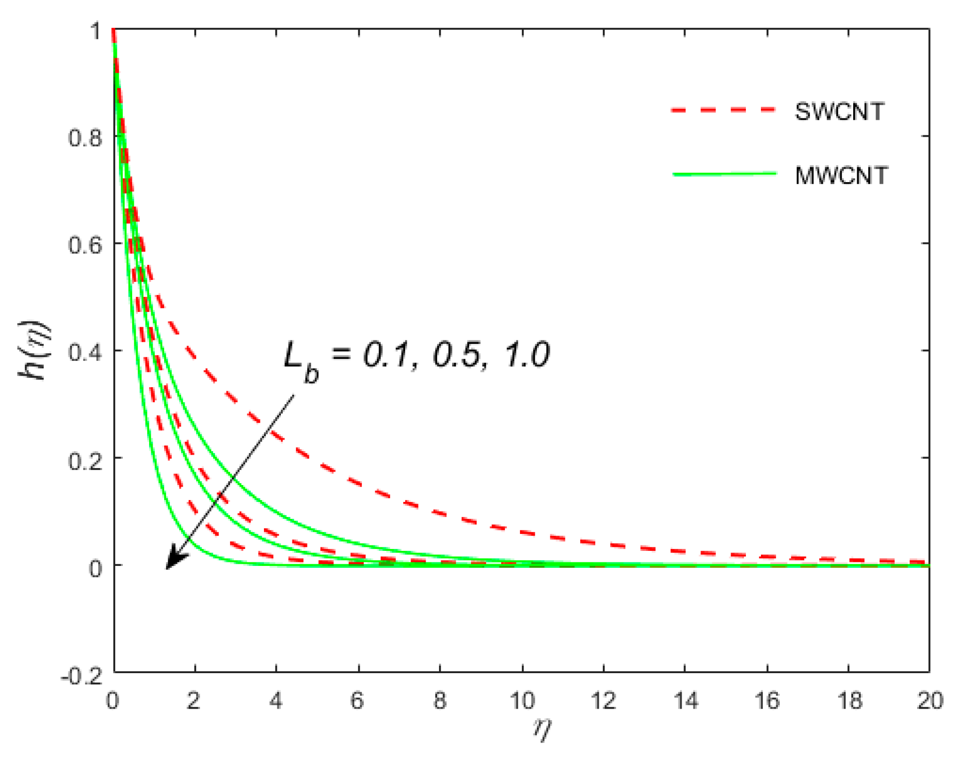
7.4. Local Density of Motile Microorganisms

The effects of (δ), (Pe), and (L_b) on Local density of motile microorganism’s profile h(η) appear in Figure 17, Figure 18 and Figure 19. The impact of bio-convection constant δ on h(η) is shown in Figure 17. The higher value of δ reduces h(η) for both Maxwell micropolar nanotubes. The influences of Pe and L_b are presented in Figure 18 and Figure 19. Decreasing behavior are observed for both L_b and Pe.

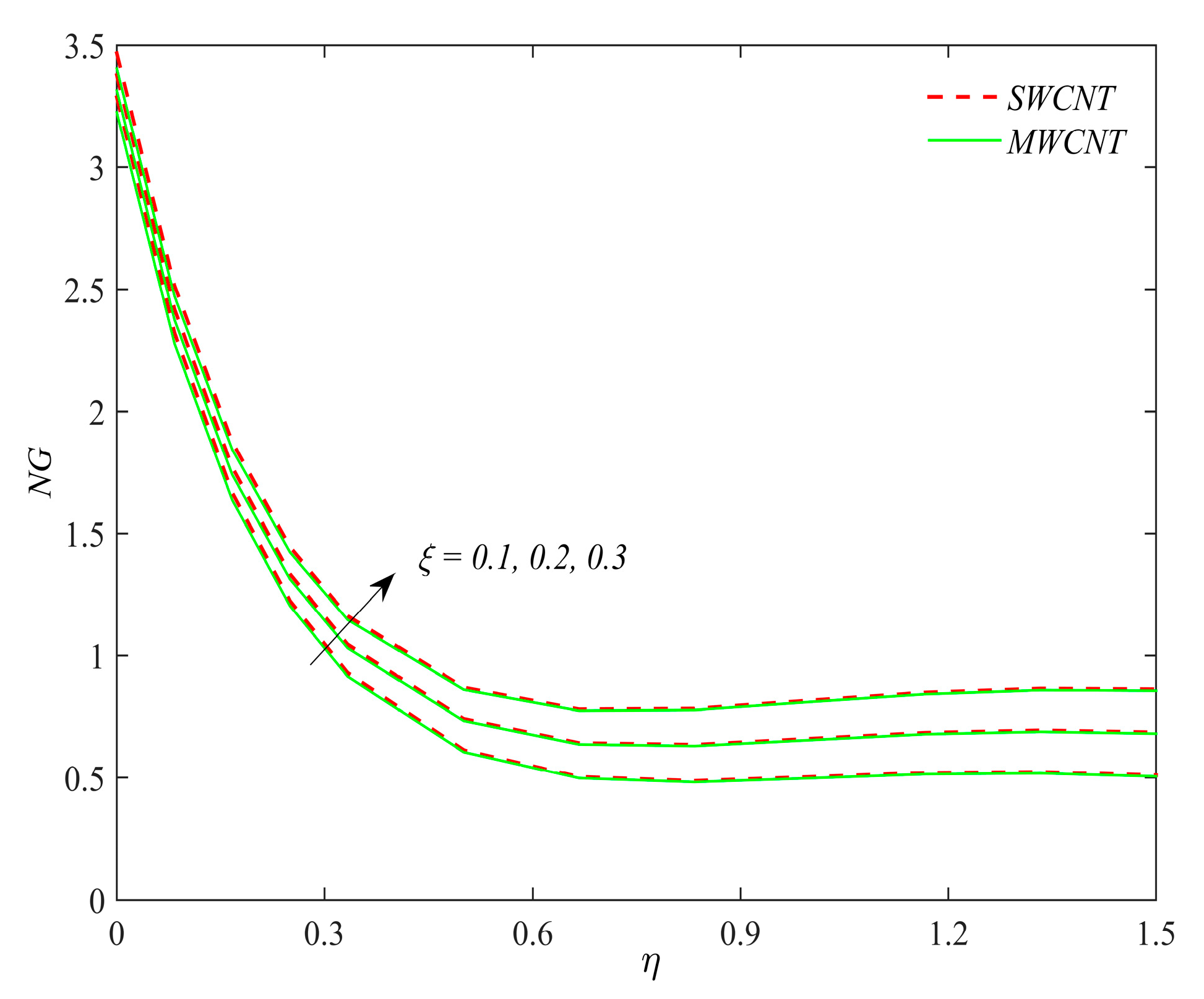
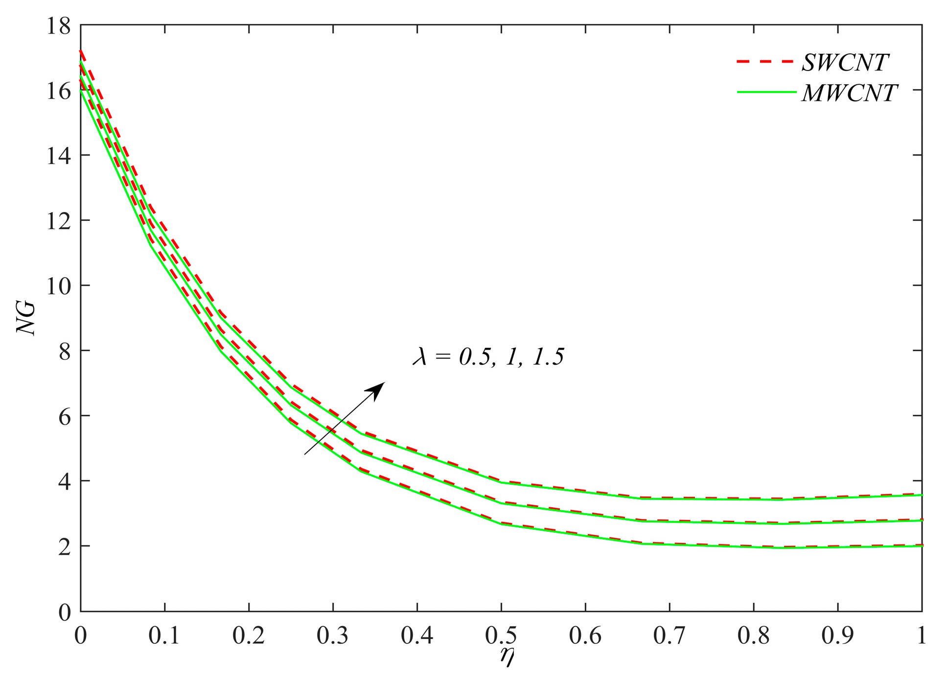
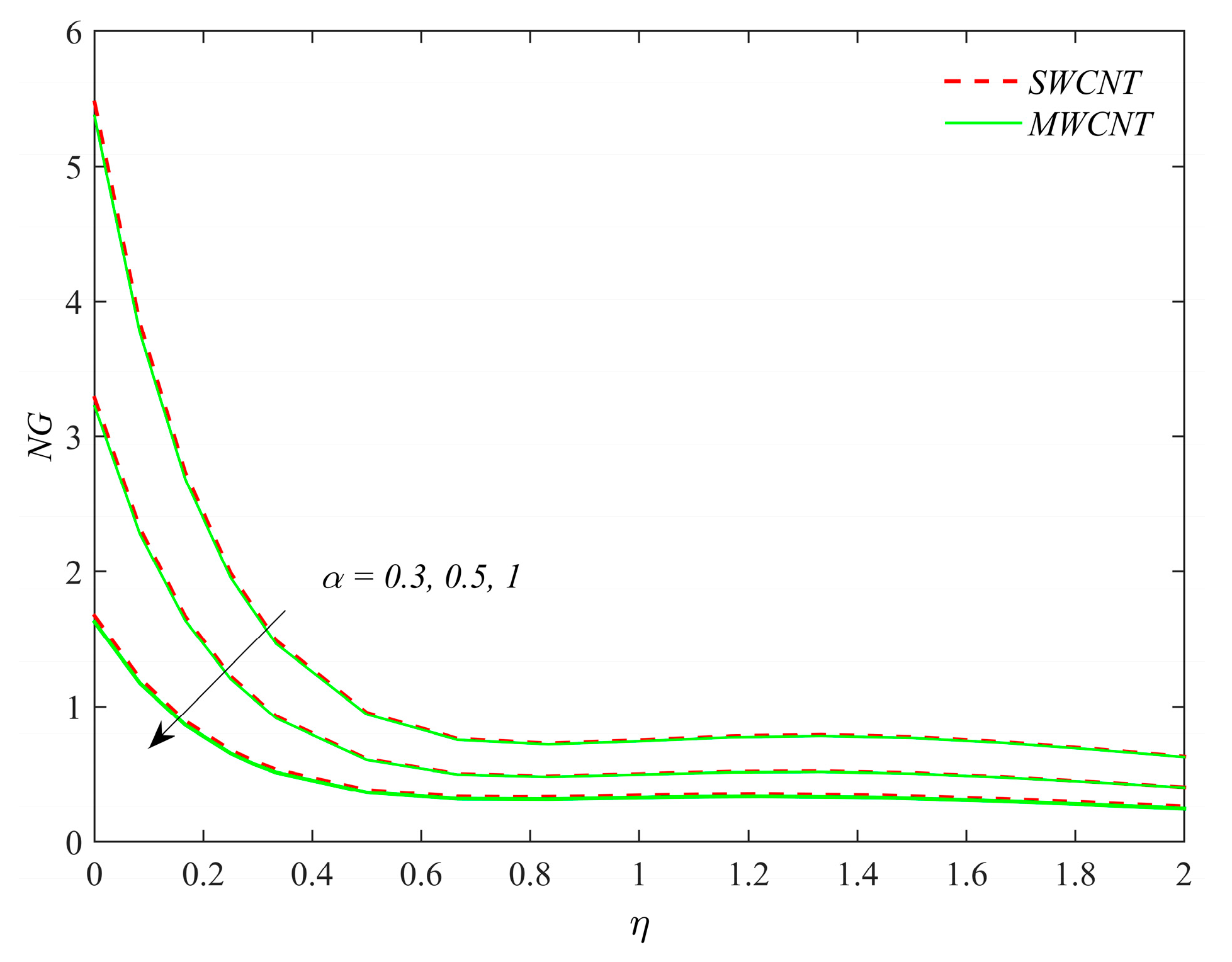
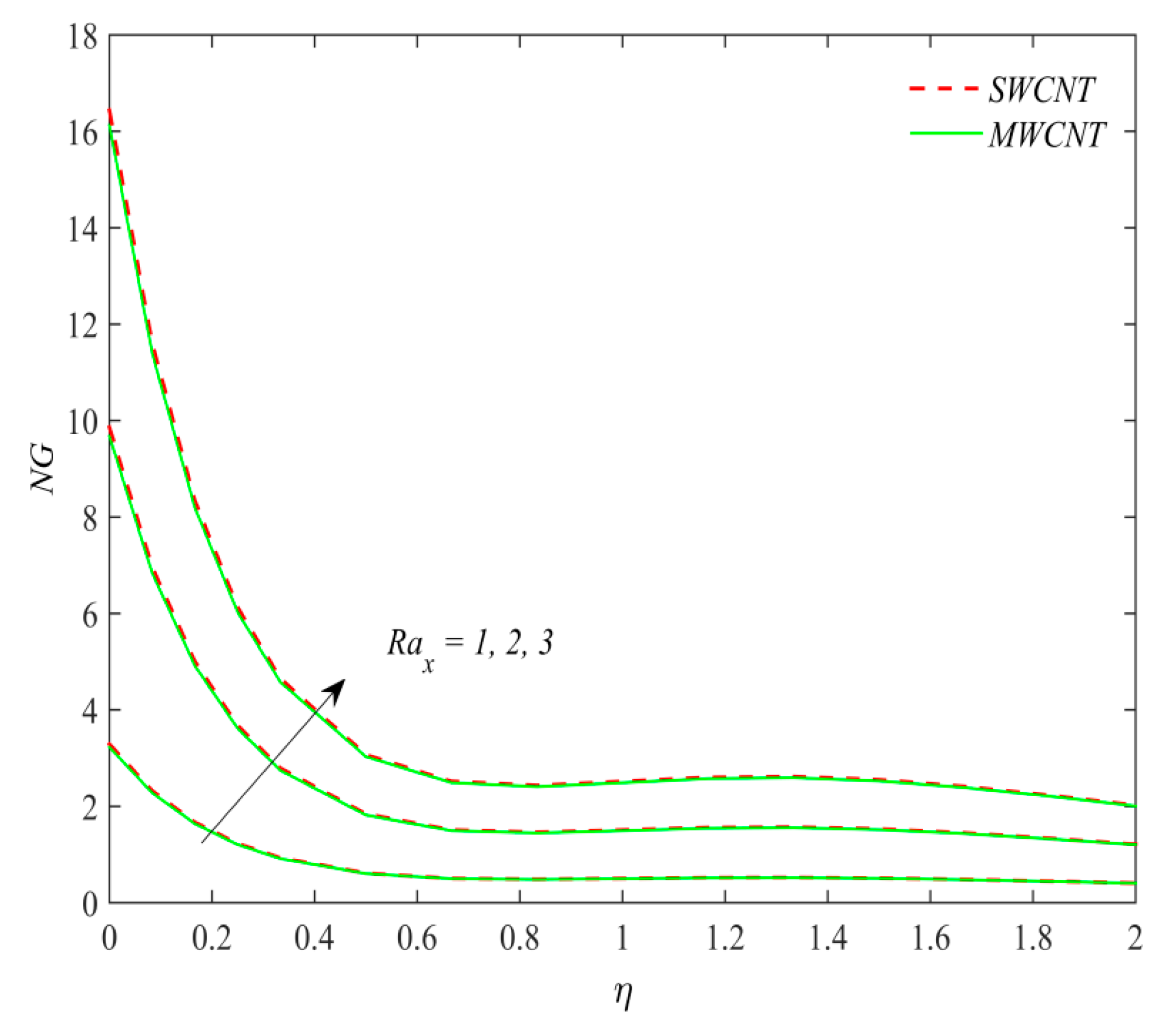
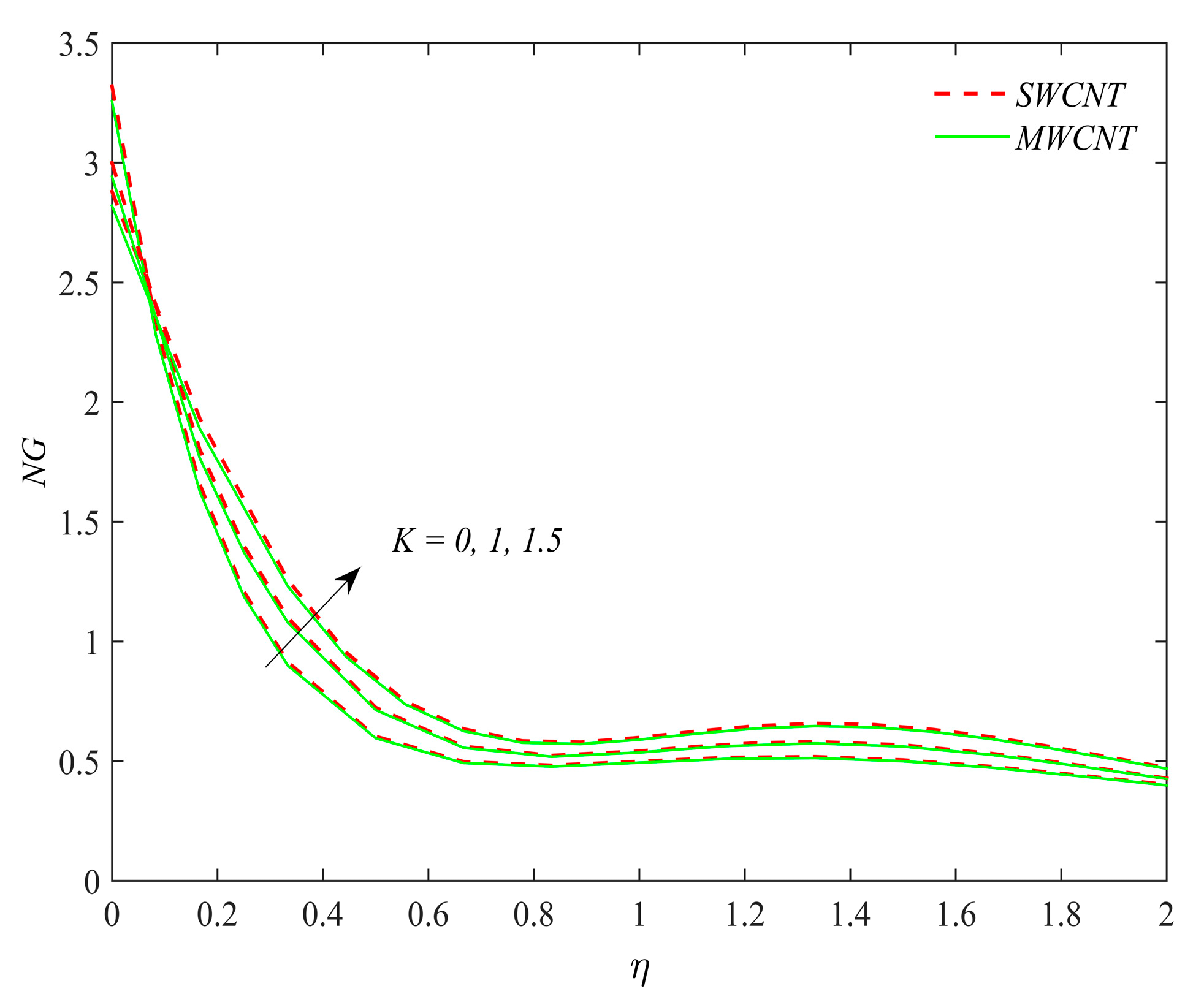
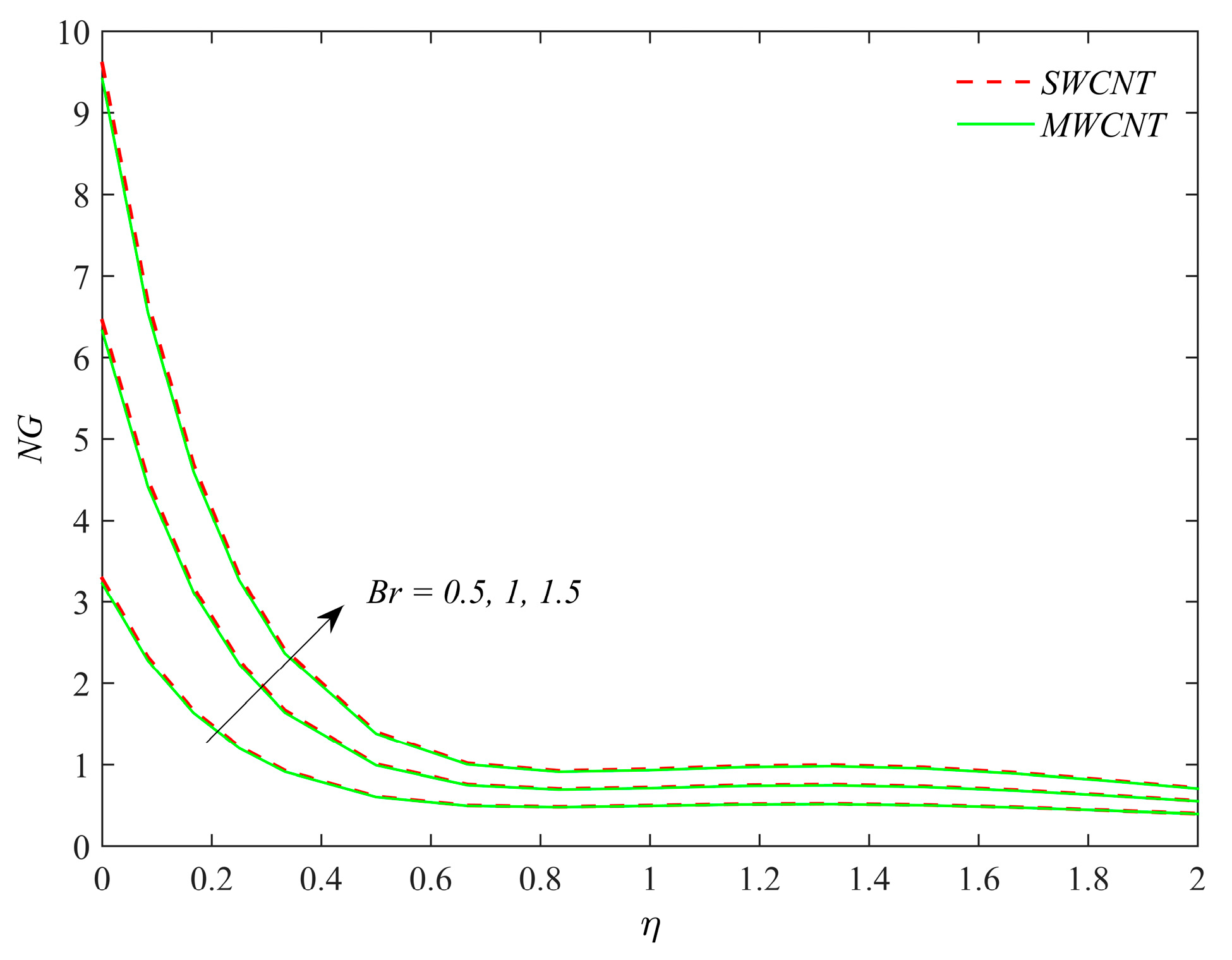
7.5. Entropy Optimization

The meddled parameters ξ, λ, α, Ra_x, K, and Br on NG are exposed in Figure 20, Figure 21, Figure 22, Figure 23, Figure 24 and Figure 25. Figure 20 and Figure 21 illustrate the variation of ξ and λ on NG. The increasing value of concentration difference ξ and diffusive constant λ enhances the entropy NG of the nanofluid of SWCNTS and MWCNTS. The Significant effects of α on NG are illustrated in Figure 22. For a higher value of parameter α the entropy NG is found as decreasing function. Figure 23 and Figure 24 show the impact of Reynold number Ra_x and micro rotation parameter K. Entropy optimization of CNTs nanofluid increases with increasing of Ra_x and K. In Figure 25 the impact of Brinkman number Br is introduced. As a matter of fact, Brinkman number is a heat produced source inside the liquid moving district. The heat produced along with the heat moves from the divider and expands the entropy optimization.

7.6. Engineering Quantities

Performances of dissimilar engineering parameter on skin friction coefficient C_Fx, temperature gradient Nu_x, mass transfer Sh_x, and local density of motile microorganisms N_nx are presented in

Table 2. Thermo-physical properties of base fluid and both type of carbon nanotubes (CNTs) i.e., SWCNTs and MWCNTs.

Material	Water	SWCNT	MWCNT
Cp (j/kgK)	4179	425	796
ρ (kg/m3)	997.1	2600	1600
k (W/mK)	0.613	6600	3000

,

Table 3. Estimations of skin friction $f^{″}(0)$ versus different evaluations of various parameters.

Φ	k1	V0	Rb	C	$\frac{1}{{\left(1-\mathsf{\varphi }\right)}^{2.5}}{\mathit{f}}^{″}(\mathbf{0})$
					SWCNTs	MWCNTs
0.01	0.5	1.0	0.1	0.1	1.8355	1.7511
0.03	–	–	–	–	2.2996	1.8007
0.05	–	–	–	–	2.4875	1.8673
–	0.5	–	–	–	1.1596	1.1465
–	0.7	–	–	–	1.4990	1.4987
–	0.9	–	–	–	1.8355	1.8165
–	–	0.5	–	–	2.8463	2.7389
–	–	0.6	–	–	2.5630	2.5314
–	–	0.7	–	–	2.3591	2.3284
–	–	–	0.2	–	2.9477	2.2959
–	–	–	0.3	–	1.9302	1.9281
–	–	–	0.4	–	1.9201	1.8890
–	–	–	–	0.1	2.1976	2.0633
–	–	–	–	0.2	2.0917	2.0528
–	–	–	–	0.3	2.0750	2.0450

,

Table 4. Estimations of Nusselt number $-\frac{k_{nf}}{k}\left(1+R_d\right){\mathsf{\theta }}^{\prime }(\mathbf{0})$ different evaluations of various parameters.

Φ	Rd	B1	M	Ec	$-\frac{{\mathit{k}}_{\mathit{n}\mathit{f}}}{\mathit{k}}\left(1+{\mathit{R}}_{\mathit{d}}\right){\mathsf{\theta }}^{\prime }(0)$
					SWCNTs	MWCNTs
0.01	0.1	1.0	0.1	0.5	0.0122	0.0138
0.03	–	–	–	–	0.0200	0.0142
0.05	–	–	–	–	0.0222	0.0153
–	0.2	–	–	–	0.0205	0.0323
–	0.3	–	–	–	0.0232	0.0181
–	0.4	–	–	–	0.0290	0.0160
–	–	0.5	–	–	0.0134	0.0133
–	–	0.7	–	–	0.0137	0.0138
–	–	1.0	–	–	0.0139	0.0177
–	–	–	0.1	–	0.0122	0.0119
–	–	–	0.2	–	0.0139	0.0138
–	–	–	0.3	–	0.0142	0.0141
–	–	–	–	0.1	0.0116	0.0115
–	–	–	–	0.5	0.0139	0.0138
–	–	–	–	1.0	0.0159	0.0158

,

Table 5. Estimations of Sherwood number $-g^{\prime }(0)$ versus different evaluations of various parameters.

Sc	Gr	n	Nr	$-{\mathit{g}}^{\prime }(\mathbf{0})$
				SWCNTs	MWCNTs
0.1	0.1	0.1	0.5	0.3430	0.3428
0.5	–	–	–	0.6290	0.6102
0.9	–	–	–	0.9227	0.8932
–	0.1	–	–	0.6290	0.6102
–	0.2	–	–	0.6977	0.6972
–	0.3	–	–	0.7513	0.7508
–	–	0.0	–	0.6290	0.6274
–	–	0.1	–	0.6147	0.6102
–	–	0.2	–	0.5782	0.6066
–	–	–	0.6	0.6072	0.6187
–	–	–	0.7	0.6005	0.6589
–	–	–	0.8	0.5954	0.6033

and

Table 6. Values of Motile density number $-h^{\prime }(0)$ versus various estimates of different parameters.

Lb	Pe	Rb	δ	$-{\mathit{h}}^{\prime }(\mathbf{0})$
				SWCNTs	MWCNTs
0.5	0.5	0.1	0.1	0.7525	0.7515
0.6	–	–	–	0.8386	0.8375
0.7	–	–	–	0.9640	0.8806
–	0.1	–	–	0.5504	0.5175
–	0.2	–	–	0.5602	0.5760
–	0.3	–	–	0.6074	0.6779
–	–	0.0	–	0.7493	0.7483
–	–	0.1	–	0.7441	0.7789
–	–	0.2	–	0.7493	0.7847
–	–	–	0.6	0.7792	0.7515
–	–	–	0.7	0.7996	0.8050
–	–	–	0.8	0.8494	0.8231

. Various Thermal-physical properties of carbon nanotubes are shown in Table 2.

7.7. Surface Drag Force

Table 3 show the numerical variation in term of skin friction C_Fx. Numerical variation of Φ, k₁, V₀, R_b, and M are shown. It is observed that the higher value of Φ, k₁, V₀, and R_b augmented the surface drag force C_Fx for both SWCNTs and MWCNTs while the opposite impact is found for M.

7.8. Heat Transfer Rate

Table 4 show numerical variation in Nusselt number Nu_x. Numerical variation of Φ, R_d, B₁, Ec, and M are shown. It is observed that the higher value of Φ, R_d, B₁, Ec, and M augmented the heat transfer rate for both SWCNTs and MWCNTs.

7.9. Mass Transfer Rate

Table 5 show the numerical variation in Sherwood number Sh_x. Numerical variation of Sc, G_r, n, and N_r are shown. It is observed that the higher value of Sc, G_r, n, and N_r augmented the mass transfer rate Sh_x in both SWCNTs and MWCNTs while the opposite impact is found for N_r.

7.10. Local Density of Motile Microorganisms N_nx

Table 6 shows the numerical variation in local density of motile microorganisms N_nx. Numerical variation of L_b, Pe, R_b, and δ are shown. It is observed that the higher value of L_b, Pe, R_b, and δ augmented the local density of motile microorganisms both SWCNTs and MWCNTs while the opposite impact is found for N_r.

8. Conclusions

In this article we studied the flow of two vertical conical carbon nanotubes (SWCNT and MWCNT) under the action of aqueous nanofluids, accompanied by the movement of swirling microorganisms and the influence of solute stratification in porous media. The investigation is carried out in the presence of chemical reactions, heat generation/absorption, and Joule heating. The noticeable features of the modeled problem are:

• The motion of the nanoparticle increases for enlarging values of solid volume fraction (Φ).
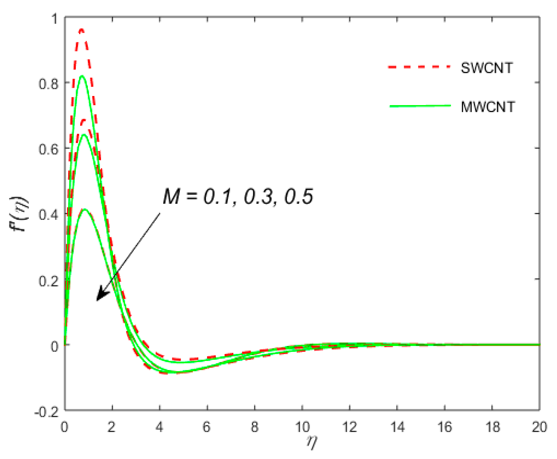
• For a larger value of magnetic parameter (M) the Lorentz forces enhance which raises the forces of resistance of the Maxwell micropolar motion which in turn reduces velocity f′(η).
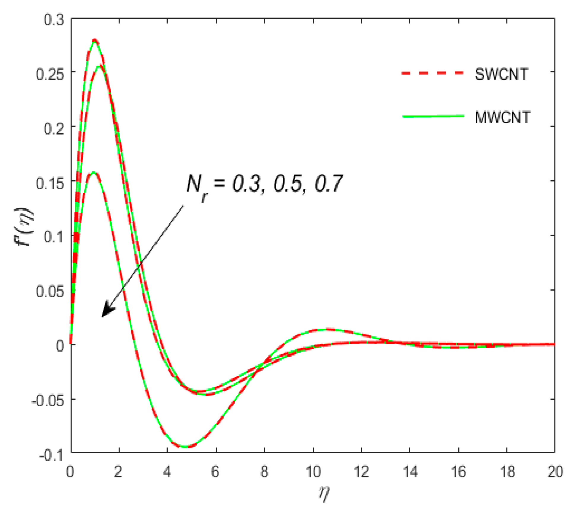
• The augmented N_r reduced the fluid motion.
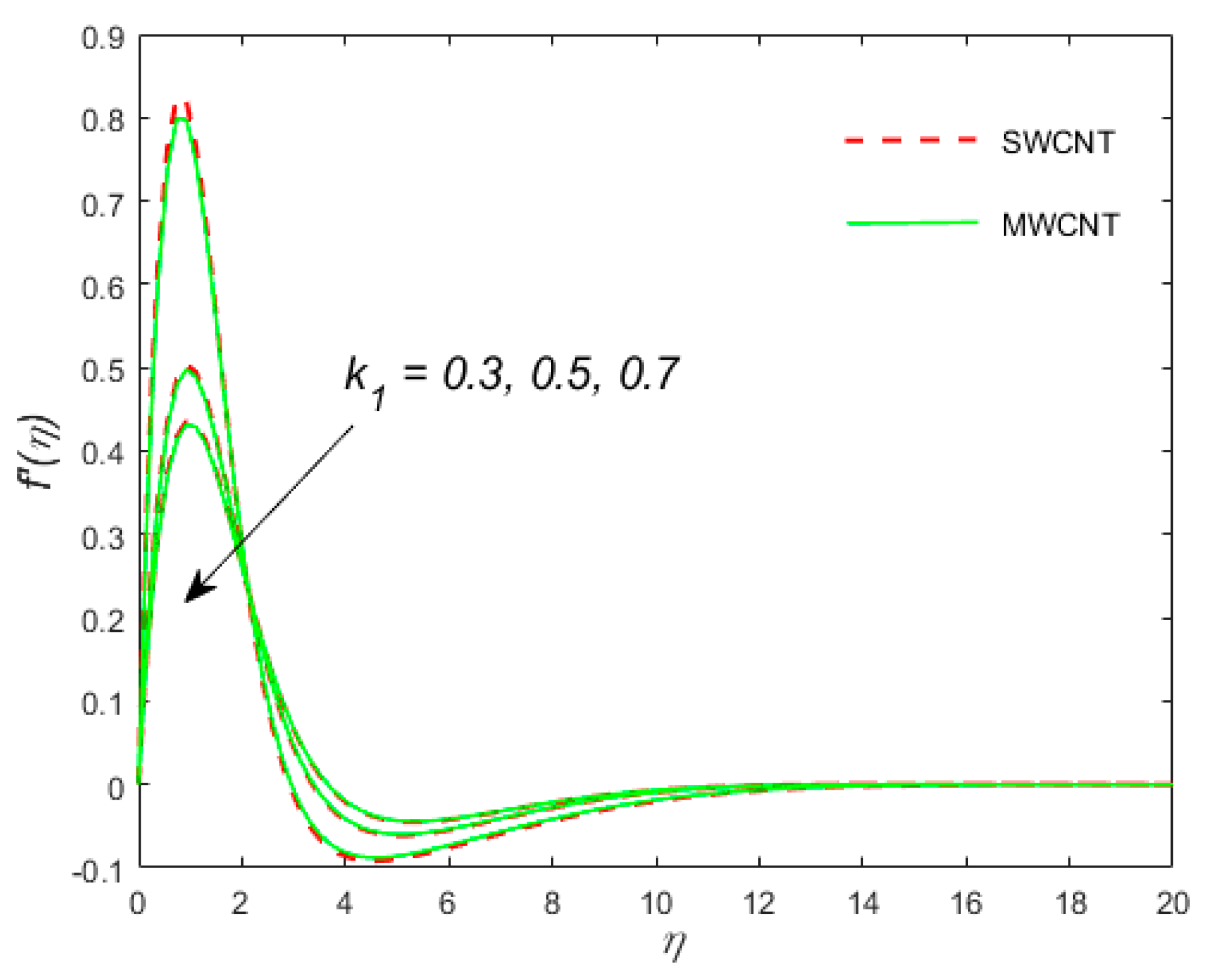
• The momentum boundary layer reduces with enhances value of k₁.
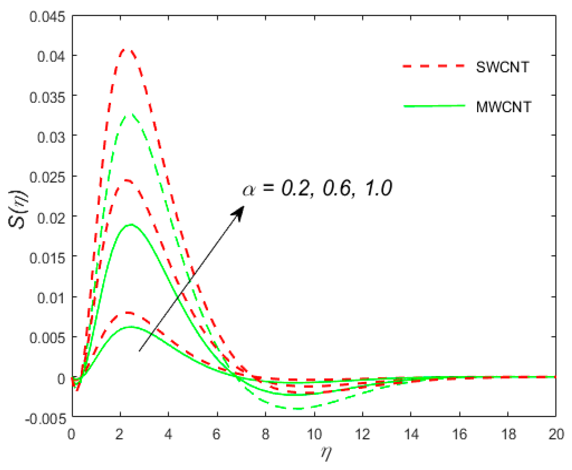
• Micro rotation velocity S(η) augmented with a higher value of K, γ*, and α.
• Augmentation in the θ(η) with enhancement radiation parameter R_d is observed.
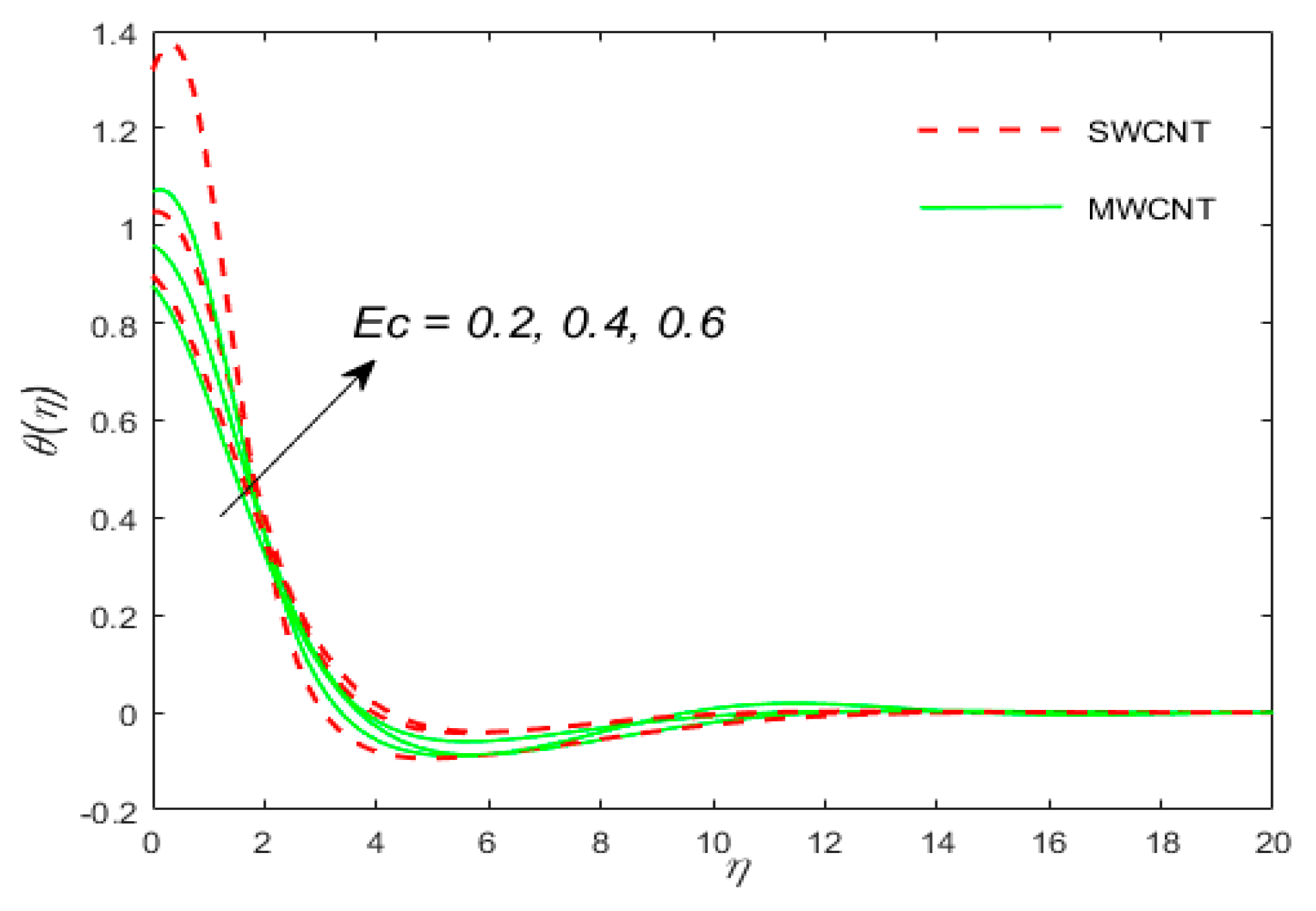
• The higher value of Ec amplified the kinetic energy of CNTs Maxwell micropolar nanofluid molecules, which thus enhanced the heat transmission rate.
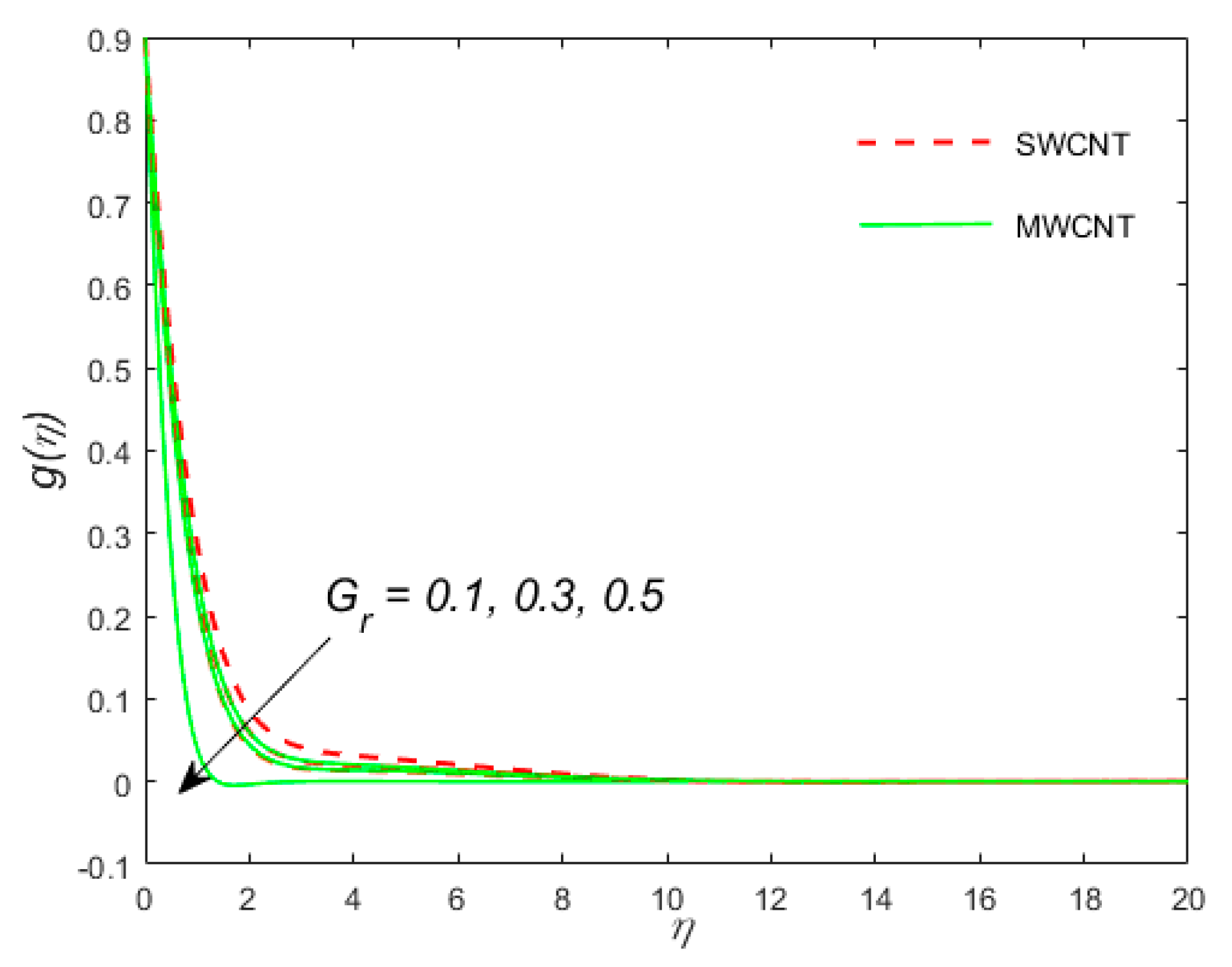
• The augmented rate of G_r reduces the concentration of Maxwell micropolar nanofluid.
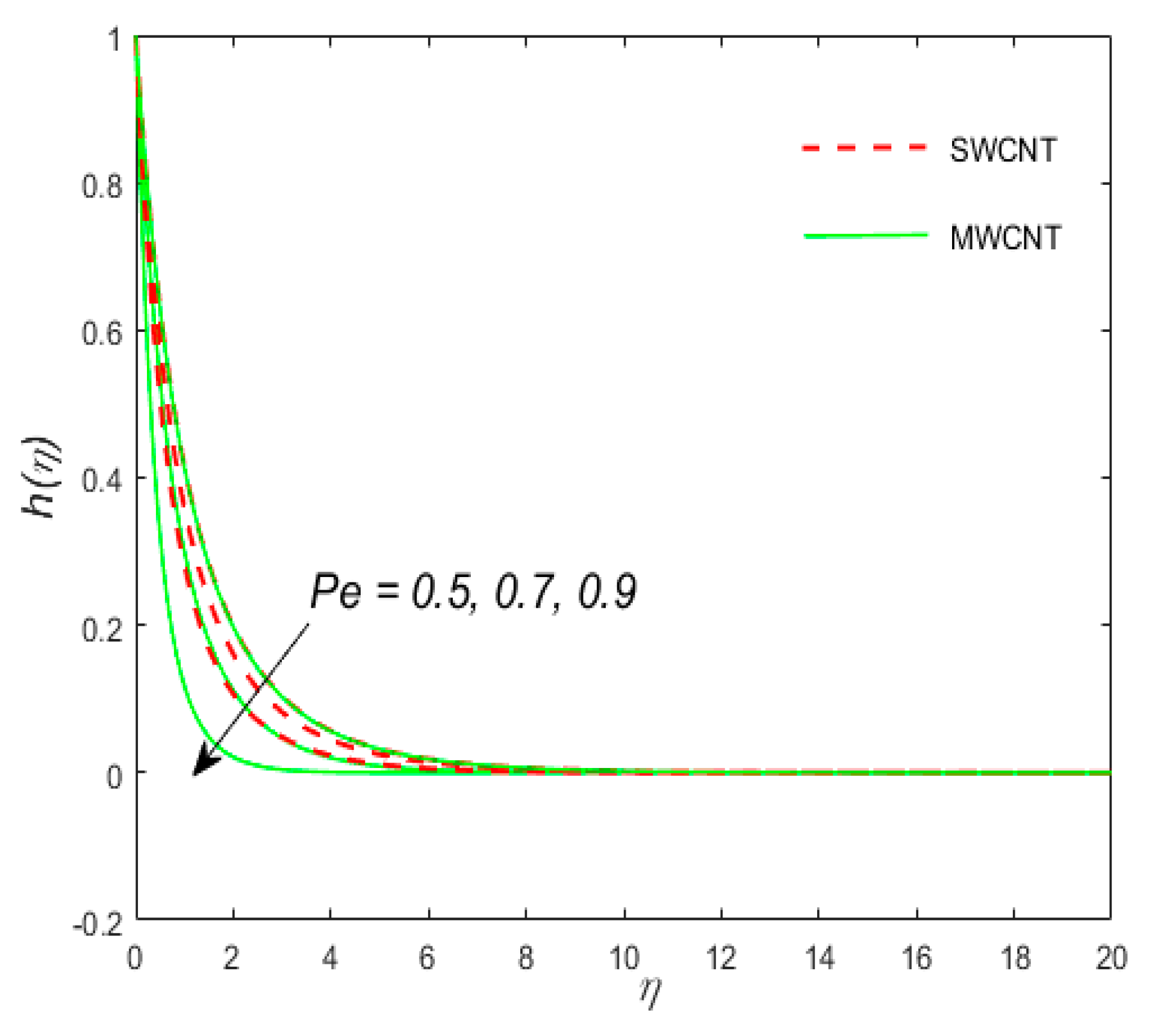
• As the estimate of the number of Peclets increases, the number of motion densities also increases.
• With the rise in estimations of Pe, h(η) are increases.
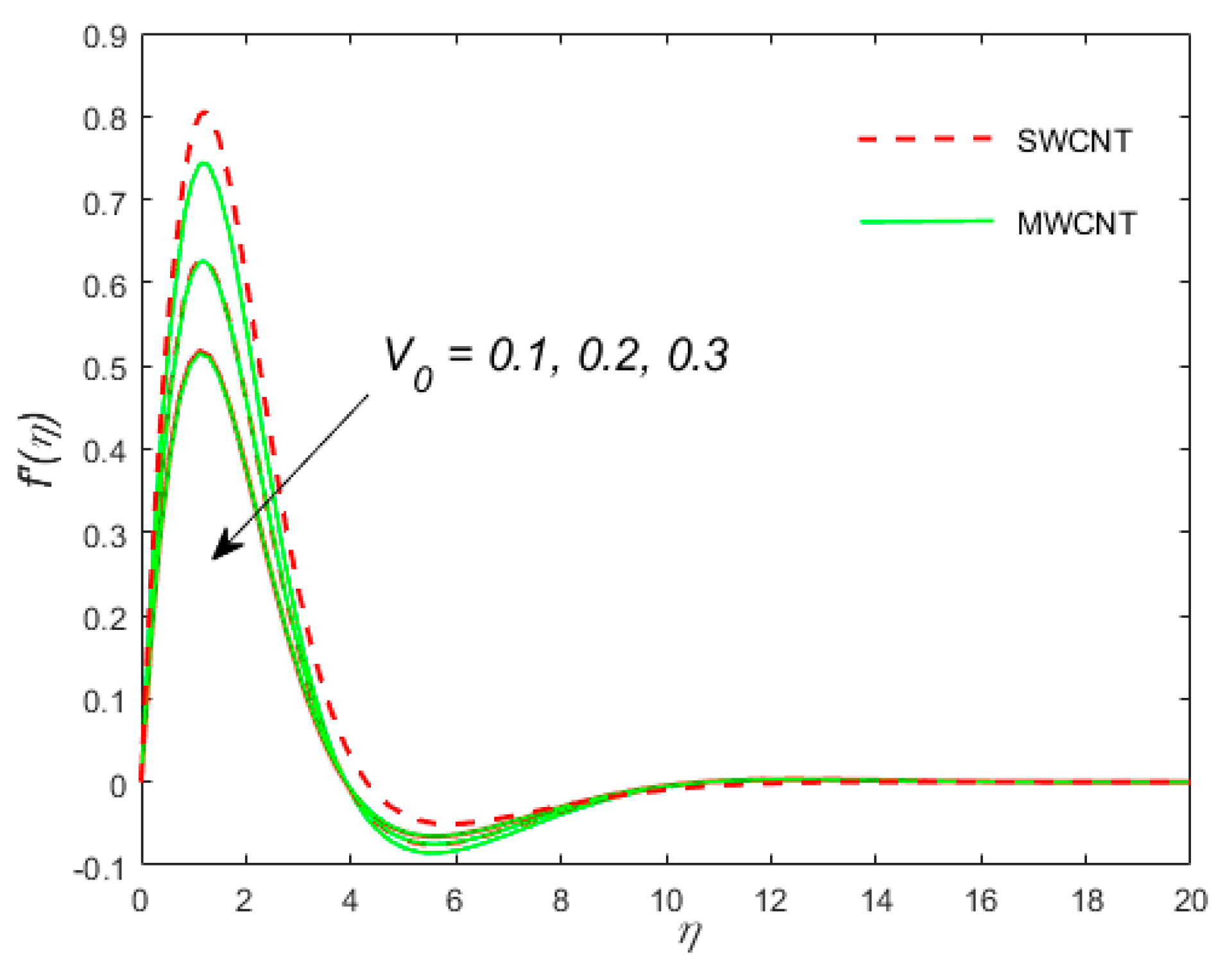
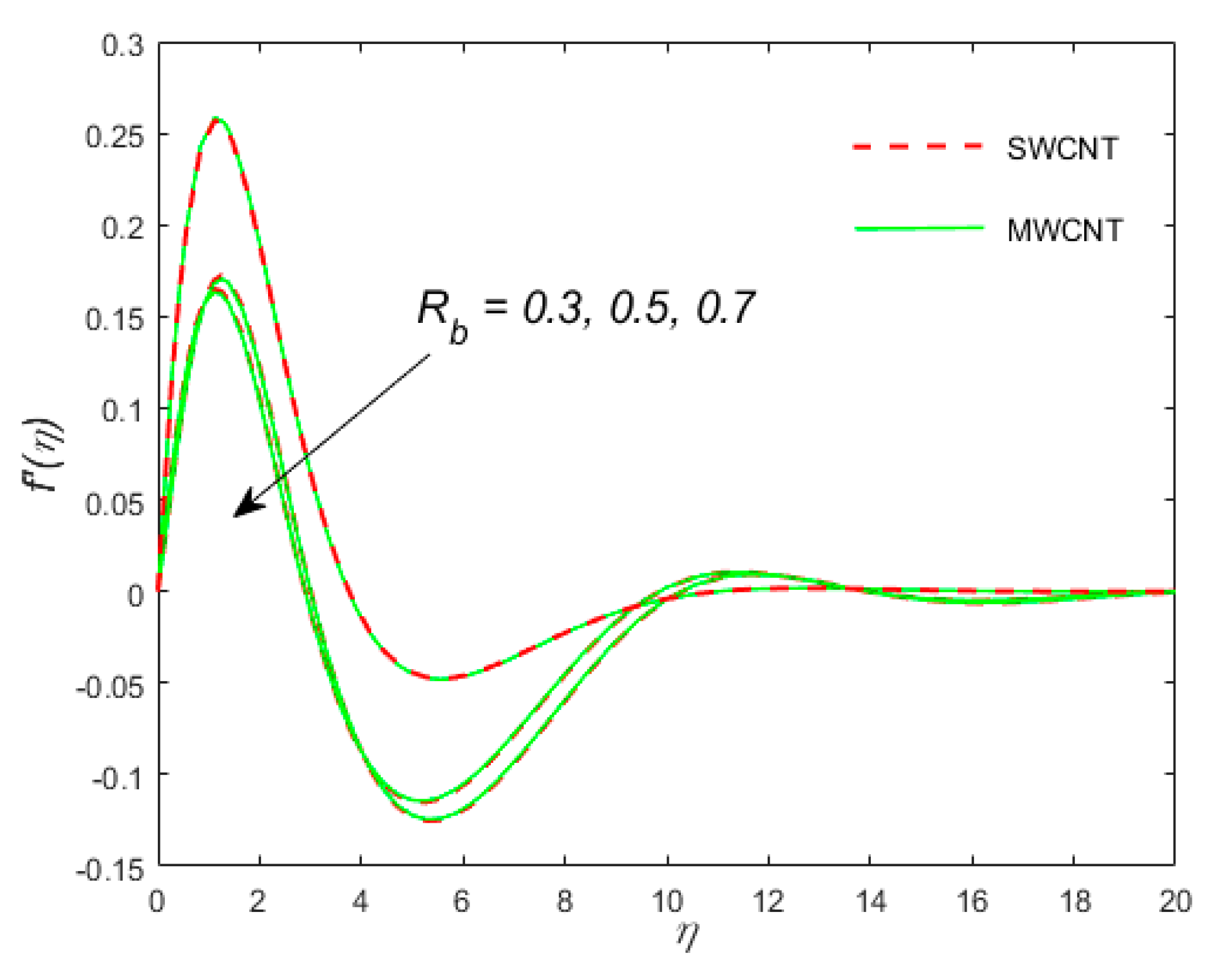
• For both CNTs, f′(η) intensifies against rising values of suction. For rising values of N_r, θ(η) is reducing.
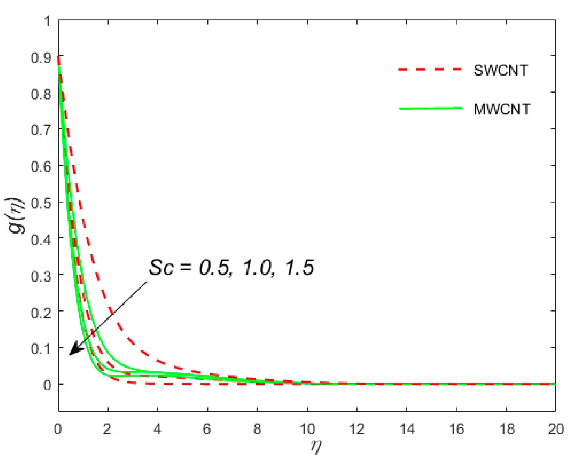
• For these CNTs, g(η) is reduced on the increasing of n.
• For the growth estimates of N_r, Sh_x is reduced and raises against numerical values of C_r.
• For solid volume fraction C_f is increased.
• Magnetic force M reduces Nu_x.
• A comparison between the present and previous outcomes for justification is given in Table 1.

References

1. Choi, S.U.; Eastman, J.A. Enhancing Thermal Conductivity of Fluids with Nanoparticles; Argonne National Lab: Lemonte, IL, USA, 1995. [Google Scholar]
2. Chen, L.; Liu, J.; Fang, X.; Zhang, Z. Reduced graphene oxide dispersed nanofluids with improved photo-thermal conversion performance for direct absorption solar collectors. Sol. Energy Mater. Sol. Cells 2017, 163, 125–133. [Google Scholar] [CrossRef]
3. Oudina, F.M. Convective heat transfer of Titania nanofluids of different base fluids in cylindrical annulus with discrete heat source. Heat Transf. Asian Res. 2019, 48, 135–147. [Google Scholar] [CrossRef] [Green Version]
4. Oudina, F.M. Numerical modeling of the hydrodynamic stability in vertical annulus with heat source of different lengths. Eng. Sci. Technol. Int. J. 2017, 20, 1324–1333. [Google Scholar]
5. Sheikholeslami, M.; Shah, Z.; Shafee, A.; Khan, I.; Tlili, T. Uniform magnetic force impact on water based nanofluid thermal behavior in a porous enclosure with ellipse shaped obstacle. Sci. Rep. 2019, 1196. [Google Scholar] [CrossRef] [Green Version]
6. Chougule, S.S.; Nirgude, V.V.; Gharge, P.D.; Mayank, M.; Sahu, S.K. Heat Transfer enhancements of low volume concentration CNT/water nanofluid and wire coil inserts in a circular tube. Energy Procedia 2016, 90, 552–558. [Google Scholar] [CrossRef]
7. Herrmann-Priesnitz, B.; Calderón-Muñoz, V.R.; Valencia, A.; Soto, R. Thermal design exploration of a swirl flow microchannel heat sink for high heat flux applications based on numerical simulations. Appl. Therm. Eng. 2016, 109, 22–34. [Google Scholar] [CrossRef]
8. Ding, Y.; Alias, H.; Wen, D.; Williams, R.A. Heat transfer of aqueous suspensions of carbon nanotubes (CNT nanofluids). Int. J. Heat Mass Transf. 2006, 49, 240–250. [Google Scholar] [CrossRef]
9. Pop, I.; Watanabe, T. Free convection with uniform suction or injection from a vertical cone for constant wall heat flux. Int. Commun. Heat Mass Transf. 1992, 19, 275–283. [Google Scholar] [CrossRef]
10. Xu, H. Modelling unsteady mixed convection of a nanofluid suspended with multiple kinds of nanoparticles between two rotating disks by generalized hybrid model. Int. Comm. Heat Mass Tran. 2019, 108, 104275. [Google Scholar] [CrossRef]
11. Rohsenow, W.M.; Hartnett, J.P.; Cho, Y.I. Handbook of Heat Transfer; McGraw-Hill Book Co.: New York, NY, USA, 1985. [Google Scholar] [CrossRef]
12. Sharma, K.V.; Sundar, L.S.; Sarma, P.K. Estimation of heat transfer coefficient and friction factor in the transition flow with low volume concentration of Al2O3 nano fluid flowing in a circular tube and with wisted tape insert. Int. Commun. Heat Mass Transf. 2009, 36, 503–507. [Google Scholar] [CrossRef]
13. Zhang, Y. Modified computational methods using effective heat capacity model for the thermal evaluation of PCM outfitted walls. Int. Commun. Heat Mass Transf. 2019, 108, 104278. [Google Scholar] [CrossRef]
14. Sun, X.; Zhang, Q.; Medina, M.A.; Lee, K.O. Experimental observations on the heat transfer enhancement caused by natural convection during melting of solid–liquid 17 phase change materials (PCMs). Appl. Energy 2016, 162, 1453–1461. [Google Scholar] [CrossRef]
15. Phuoc, T.X.; Massoudi, M.; Chen, R.H. Viscosity and thermal conductivity of nanofluids containing carbon nanotubes stabilized by Chitosan. Int. J. Therm. Sci. 2011, 50, 12–18. [Google Scholar] [CrossRef]
16. Harish, S.; Ishikawa, K.; Einarsson, E.; Aikawa, S.; Chiashi, S.; Shiomi, J.; Maruyama, S. Enhanced thermal conductivity of ethylene glycol with single-walled carbon nanotube inclusions. Int. J. Heat Mass Transf. 2012, 55, 3885–3890. [Google Scholar] [CrossRef]
17. Hayat, T.; Muhammad, T.; Shehzad, S.A.; Chen, G.Q.; Abbas, I.A. Interaction of magnetic field in flow of Maxwell nanofluid with convective effect. J. Magn. Magn. Mater. 2015, 389, 48–55. [Google Scholar] [CrossRef]
18. Bejan, A. A study of entropy generation in fundamentsl convective heat transfer. J. Heat Trans. 1979, 101, 718–725. [Google Scholar] [CrossRef]
19. Ellahi, R.; Hassan, M.; Zeeshan, A.; Khan, A.A. The shape effects of nanoparticles suspended in HFE-7100 over wedge with entropy generation and mixed convection. Appl. Nanosci. 2016, 6, 641–651. [Google Scholar] [CrossRef] [Green Version]
20. Sheikholeslami, M.; Jafaryar, M.; Hedayat, M.; Shafee, A.; Li, Z.; Khang Nguyen, T.; Bakouri, M. Heat transfer and turbulent simulation of nanomaterial due to compound turbulator including irreversibility analysis. Int. J. Heat Mass Transf. 2019, 137, 1290–1300. [Google Scholar] [CrossRef]
21. Ramzan, M.; Mohammad, M.; Howari, F. Magnetized suspended carbon nanotubes based nanofluid flow with bio-convection and entropy generation past a vertical cone. Sci. Rep. 2019, 9, 12225. [Google Scholar] [CrossRef] [PubMed]
22. Sarafraz, M.M.; Reza Safaei, M.; Goodarzi, M.; Arjomandi, M. Reforming of methanol with steam in a micro-reactor with Cu–SiO2 porous catalyst. Int. J. Hydrogen Energy 2019, 44, 19628–19639. [Google Scholar] [CrossRef]
Figure 1. Schematic diagram for the flow direction.
Coatings 10 00998 g001
Figure 2. The variation of the velocity distribution profile f′(η) for the case of SWCNT and MWCNT versus the similarity variable for the distinct values of the nanoparticle volume fraction ( ϕ ) .
Coatings 10 00998 g002
Figure 3. The variation of the velocity distribution profile f′(η) for the case of SWCNT and MWCNT versus the similarity variable for the distinct values of the magnetic parameter (M).
Coatings 10 00998 g003
Figure 4. The variation of the velocity distribution profile f′(η) for the case of SWCNT and MWCNT versus the similarity variable for the distinct values of the suction parameter (V0).
Coatings 10 00998 g004
Figure 5. The variation of the velocity distribution profile f′(η) for the case of SWCNT and MWCNT versus the similarity variable for the distinct values of the buoyancy ratio parameter (Nr).
Coatings 10 00998 g005
Figure 6. The variation of the velocity distribution profile f′(η) for the case of SWCNT and MWCNT versus the similarity variable for the distinct values of the bio-convection Rayleigh number (Rb).
Coatings 10 00998 g006
Figure 7. The variation of the velocity distribution profile f′(η) for the case of SWCNT and MWCNT versus the similarity variable for the distinct values of the porous parameter (k1).
Coatings 10 00998 g007
Figure 8. The impact of the temperature distribution profile θ(η) for the case of SWCNT and MWCNT versus the similarity variable for the distinct values of the Boit number (B1).
Coatings 10 00998 g008
Figure 9. The impact of the temperature distribution profile θ(η) for the case of SWCNT and MWCNT versus the similarity variable for the distinct values of the radiation parameter Rd.
Coatings 10 00998 g009
Figure 10. The impact of the temperature distribution profile θ(η) for the case of SWCNT and MWCNT versus the similarity variable for the distinct values of the Eckert number Ec.
Coatings 10 00998 g010
Figure 11. The impact of the temperature distribution profile θ(η) for the case of SWCNT and MWCNT versus the similarity variable for the distinct values of the magnetic parameter M.
Coatings 10 00998 g011
Figure 12. The variation of the micro rotation profile S(η) for the case of SWCNT and MWCNT versus the similarity variable for the distinct values of the material parameter K.
Coatings 10 00998 g012
Figure 13. The variation of the micro rotation profile S(η) for the case of SWCNT and MWCNT versus the similarity variable for the distinct values of the vortex velocity or material parameter γ*.
Coatings 10 00998 g013
Figure 14. The variation of the micro rotation profile S(η) for the case of SWCNT and MWCNT versus the similarity variable for the distinct values of the temperature difference parameter α.
Coatings 10 00998 g014
Figure 15. The variation of the concentration profile g(η) for the case of SWCNT and MWCNT versus the similarity variable for the distinct values of the Schmidt number Sc.
Coatings 10 00998 g015
Figure 16. The variation of the concentration profile g(η) for the case of SWCNT and MWCNT versus the similarity variable for the distinct values of the chemical response factor Gr.
Coatings 10 00998 g016
Figure 17. The variation of the local density of motile microorganisms h(η) for the case of SWCNT and MWCNT versus the similarity variable for the distinct values of the bio-convection constant δ.
Coatings 10 00998 g017
Figure 18. The variation of the local density of motile microorganisms h(η) for the case of SWCNT and MWCNT versus the similarity variable for the distinct values of the bio-convection Peclet number Pe.
Coatings 10 00998 g018
Figure 19. The variation of the local density of motile microorganisms h(η) for the case of SWCNT and MWCNT versus the similarity variable for the distinct values of the bio-convection Lewis number Lb.
Coatings 10 00998 g019
Figure 20. The variation of the entropy optimization NG for the case of SWCNT and MWCNT versus the similarity variable for the distinct values of the concentration difference parameter ξ.
Coatings 10 00998 g020
Figure 21. The variation of the entropy optimization NG for the case of SWCNT and MWCNT versus the similarity variable for the distinct values of the diffusive constant parameter λ.
Coatings 10 00998 g021
Figure 22. The variation of the entropy optimization NG for the case of SWCNT and MWCNT versus the similarity variable for the distinct values of the temperature difference parameter α.
Coatings 10 00998 g022
Figure 23. The variation of the entropy optimization NG for the case of SWCNT and MWCNT versus the similarity variable for the distinct values of the Reynold number Rax.
Coatings 10 00998 g023
Figure 24. The variation of the entropy optimization NG for the case of SWCNT and MWCNT versus the similarity variable for the distinct values of the material parameter K.
Coatings 10 00998 g024
Figure 25. The variation of the entropy optimization NG for the case of SWCNT and MWCNT versus the similarity variable for the distinct values of the Brinkman number Br.
Coatings 10 00998 g025