Sliding Dispersion Entropy-Based Fault State Detection for Diaphragm Pump Parts

Abstract

Aiming at the disadvantages of low trend, poor characterization performance, and poor anti-noise performance of traditional degradation features such as dispersion entropy (DE), a fault detection method based on sliding dispersion entropy (SDE) is proposed. Firstly, a sliding window is added to the signal before extracting the DE feature, and the root mean square of the signal inside the sliding window is used to replace the signal in the window to realize down sampling, which enhances the trend of DE. Secondly, the hyperbolic tangent sigmoid function (TANSIG) is introduced to map the signals to different categories when extracting the DE feature, which is more in line with the signal distribution of mechanical parts and the monotonicity of the degradation feature is improved. For noisy signal, the introduction of locally weighted scatterplot smoothing (LOWESS) can remove the burrs and fluctuations of the SDE curve, and the anti-noise performance of SDE is improved. Finally, the SDE state warning line is constructed based on the 2σ criterion, which can determine the fault warning point in time and effectively. The state detection results of bearing and check valve show that the proposed SDE improves the trend, monotonicity, and robustness of the state tracking curve, and provides a new method for fault state detection of mechanical parts.

1. Introduction

Diaphragm pump is a kind of transmission power equipment in the metallurgical industry, which provides power for slurry pipeline transmission. The safe operation of the diaphragm pump ensures the supply of mineral raw materials, and improves the production efficiency and the quality of steel products. The poor operating environment, stress, and load will cause damage to the diaphragm pump, which cause significant economic losses [1]. Therefore, the maintenance of the diaphragm pump is important. Bearing and check valve are the most frequently damaged parts in diaphragm pump, and the price of check valve is high. The maintenance personnel often detect the faults of bearing and check valve through abnormal sounds of diaphragm chamber and bearing seat, slurry leakage trace, pressure, and flow. These methods rely on subjective experience seriously. The excessive maintenance will cause the risk of shutdown, and the frequent replacement will cause the waste of spare parts, which will cause serious economic losses. Insufficient maintenance will lead to mechanical failure. Besides, a too late replacement of parts will lead to secondary failure of other parts, which will bring immeasurable losses and safety accidents. Therefore, it is urgent to propose a reliable fault detection method to guide the formulation of maintenance and replacement strategy.

Tracking the fault state of parts and determining the early fault point have important guiding significance for the design, assembly, and maintenance of the diaphragm pump. The time domain, frequency domain, and time-frequency domain features of the vibration signal excited by faults will change in real time with the state degradation. However, it is difficult to track and detect the fault states of the diaphragm pump because the vibration signal is interfered by the pulsation of the slurry and the vibration of parts. In addition, the signal has nonlinear and non-stationary characteristics due to the influence of transmission path and hydraulic, mechanical, and electrical factors, which brings great challenges to the fault state tracking and detection.

There are few researches on fault detection of diaphragm pumps at home and abroad, but the researches on bearing fault detection still have good reference significance. Mixed domain features are the most commonly used methods in fault detection, including time domain, frequency domain, and time-frequency domain features. Li extracted 24 time-frequency features and selected sensitive feature through monotonicity and correlation coefficient, finally tracked the bearing degradation state through gate recurrent unit and 3σ criteria [2]. Gao extracted the degradation features from the mixed domain features of the bearing through isometric mapping, then established a reliability model by logistic regression [3]. Hua extracted the mixed domain features of the bearing and constructed a fault warning line based on the 3σ principle, and finally predicted the degradation state through the support vector machine [4]. Li selected the effective features from the mixed domain features of bearing and obtained a degradation curve by self-organizing feature mapping [5]. Bilendo extracted the mixed domain features and selected effective degradation features through local linear embedding (LLE) [6]. However, the single features, mixed domain features, and its fusion features have not achieved satisfactory results in the fault detection of the bearing and check valve. The reasons for this are that single features are only sensitive to the specific fault in a specific stage, the fusion features are redundant and depend on dimensionality reduction methods. Besides, the construction and dimensionality reduction of mixed domain features depend on the experience of technicians. The deep learning method can solve the above problems [7]. Ding proposed a domain adaptive long short-term memory (LSTM) to predict the bearing degradation state [8]. Hu extracted modes by convolutional neural network and evaluated the bearing degradation process by fuzzy C mean clustering [9].

Although the above-mentioned deep learning-based methods can avoid the subjective experience problems in mixed domains, the time cost of deep learning is higher and neural network structure seriously affects the feature extraction performance. Entropy can measure the complexity and uncertainty of signal [10] and has the advantages of simple calculation and high calculation efficiency [11]. Kumar extracted the Shannon entropy, permutation entropy (PE) and approximate entropy (AE) degradation features of the bearing and then constructed a bearing degradation trend model by gaussian process regression [12]. Noman first separated the oscillating eigenvalues from the vibration signal, then took the PE of the oscillation signal as the bearing degradation feature [13]. Minhas obtained several modes by empirical mode decomposition, then extracted the weighted multi-scale entropy degradation features of sensitive modes by Hurst index [14]. Li proposed a degradation feature combining composite spectrum and relative entropy, which can characterize the degradation trend of hydraulic pump effectively [15]. Mostafa tracked the fault evolution process of gear and bearing through sample entropy (SE), PE, and dispersion entropy (DE) [16]. Experiments show that the DE [17] is not sensitive to noise, but sensitive to instantaneous frequency, amplitude, and sequence bandwidth, which is in line with the feature extraction requirement of vibration signal.

However, the entropy methods also have their own defects, SE is sensitive to signal length, PE ignores the amplitude information, and they both have poor anti-noise performance. Although the performance of DE is slightly better than that of single features, mixed domain features and traditional entropy features in the fault detection of diaphragm pump, DE has not achieved satisfactory results in the fault detection. The problems can be summarized as follows. Firstly, the vibration signal segment used to extract the DE feature is discontinuous and irrelevant, which greatly reduces the tendency of the degradation feature. Secondly, the results obtained by the normal cumulative distribution function (NCDF) used in the DE deviate from the actual distribution of vibration signals, which makes the traditional DE feature unable to well characterize the true characteristics of vibration signals. Thirdly, the anti-noise performance of DE degradation feature still does not meet the fault detection requirements of mechanical equipment in the actual industrial environment. In addition, there is still a lack of an effective fault point detection and early warning method, which can track the degradation state of parts in real time and warn the key fault points.

The sliding dispersion entropy (SDE) and its state warning line are proposed and used for fault state detection and degradation state tracking in this paper. In order to enhance the tendency of DE degradation feature, a sliding window is added to the signal segment and the root mean square of the signal in the window is used to replace the signal segment to achieve down-sampling. In order to improve the characterization performance of DE feature, the down-sampling sequences are mapped to different categories by introducing hyperbolic tangent sigmoid function (TANSIG) mapping. Because the TANSIG mapping is closer to the actual empirical distribution of vibration signal, the proposed SDE enhances the monotonicity of the degradation feature. To enhance the anti-noise performance, locally weighted scatterplot smoothing (LOWESS) is introduced to remove the small fluctuations and burrs of the SDE feature curve. At the same time, an adaptive early warning line based on 2σ criteria is proposed, which can determine the fault warning point effectively. In summary, the proposed method solves the above problems well. The method can track the fault state of the parts and determine the fault warning point and provide technical guidance for the maintenance and replacement of the parts.

The remainder of this paper is organized as follows: in Section 2, the theory of the proposed sliding dispersion entropy (SDE) and its fault state warning line are introduced. Then, a state detection method based on SDE is proposed, and the specific steps are described in detail. In Section 3, the effectiveness of the SDE and its state warning line is proved by analyzing the bearing data in the laboratory environment, then the proposed SDE is applied to the fault detection of check valve in the actual industrial environment, and the proposed SDE was compared with many existing methods. Finally, some conclusions are presented in Section 4.

2. Methodology

2.1. Sliding Dispersion Entropy (SDE)

The degradation process of mechanical parts lasts a long time, and the categories and boundaries of fault states are fuzzy. Therefore, it is difficult for traditional features to characterize the degradation trend of parts [18]. DE can measure the complexity and chaotic characteristics of the signal, but its performance is not very good in tracking the state of check valve and bearing. The trend of vibration data is not fully considered in DE feature, and the description of vibration data distribution characteristics by DE is not accurate enough due to the use of normal cumulative distribution function (NCDF) mapping. In addition, DE is easily disturbed by small fluctuations and noise, and the reliability of tracking is poor. Therefore, a sliding dispersion entropy (SDE) based on sliding window down-sampling and TANSIG mapping is proposed. Assuming that the vibration signal of the mechanical part at the k-th $(k=1,2,\cdots ,K)$ time point has been collected, the SDE feature of the vibration signal at the current time point can be expressed as $SD{E}_k$, and its calculation procedures are as follows.

(1) In order to enhance the trend of the vibration signal obtained at the k-th time point, a sliding window with length P is added to the signal to be analyzed at first, and then the original signal segment in the sliding window is replaced by the root mean square (RMS) value of the segment signal. In this way, down-sampling is achieved. In the sliding process of the sliding window, the sliding window reaches the next window after sliding $h=(P/2)$ sampling points each time. Wherein, the RMS of the signal segment in the $i$-th sliding window can be obtained by the following formula.

$$v_{rms}(i)=\sqrt{{\displaystyle \sum _{m=(i-1)h+1}^{(i-1)h+P}{u}^2}(m)/P},$$

(1)

$$v_{pre}(i)=v_{rms}(i)-\left({\displaystyle \sum _{i=1}^N{v}_{rms}(i)}/N\right),$$

(2)

where $N=round(M/P)$ represents the total number of windows, $M$ represents the number of data points at the k-th time point, and $v_{pre}(i)$ is the removing mean processing of the RMS values of the signal in the i-th window. Figure 1 shows the sliding window of the check valve signal when the signal length in the sliding window is $P=2000$. In this paper, $P=20$. The down-sampled signal $v_{pre}(i)(i=1,2,\cdots ,N)$ of the signal in the N sliding windows can be obtained according to the above formula.

(2) In order to improve the characterization performance of DE, the down-sampling signal are mapped to different categories by introducing TANSIG mapping, and it is used as the $SD{E}_k$ feature of the k-th time point signal. Its calculation is summarized as follows.

Step 1: Map the signal $x_j(j=1,2,\cdots ,N)$ to $c$ categories. Different from DE, the NCDF function of DE is replaced by the tan-sigmoid mapping function (TANSIG), after which the original signal $x_j$ is mapped to the range between 0 and 1, i.e., $y=\{y_1,y_2,\cdots ,y_N\},y\in (0,1)$. When the maximum or minimum value of sequence $x$ deviates far from its mean or median, most of the data in sequence $x$ is easy to be classified into a few categories, but TANSIG can solve the above problems well.

$$y_j=\frac{2}{1+e^{-2\frac{(x_j-\mu )}{\sigma }}}-1,$$

(3)

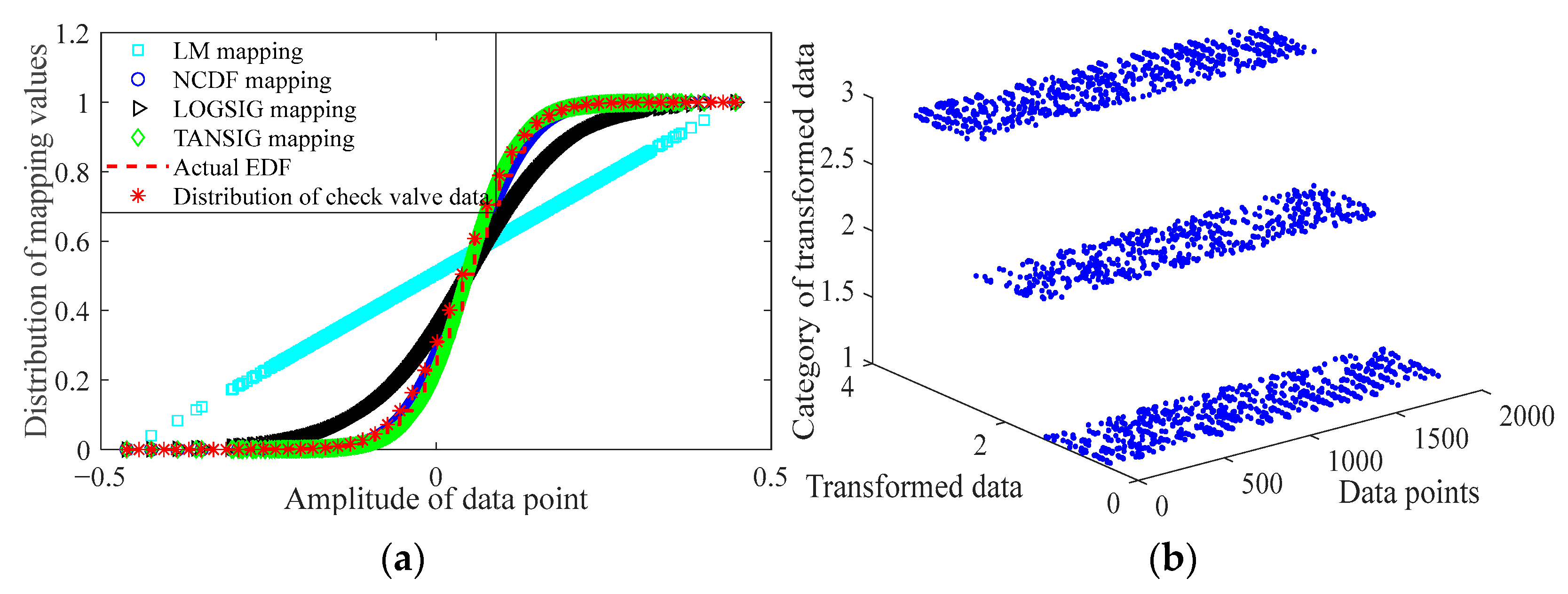
where $\sigma$ and $\mu$ are the standard deviation and mean of sequence $x$. In order to verify the effectiveness of TANSIG function, we have compared and analyzed the mapping effect and distribution of linear function (LM), log sigmoid function (LOGSIG), TANSIG function, and NCDF function based on 76,800 data points of check valve fault signal. At the same time, these functions are also compared with the actual empirical distribution function (EDF) of the check valve data. As shown in Figure 2a, the curve corresponding to the TANSIG mapping function almost coincides with the curve corresponding to the EDF function and the check valve data distribution curve, which shows that the distribution of most check valve data is closer to the TANSIG mapping function.

Then, the vibration data points are transformed into the range of 1 to $c$ by the linear transformation $c·y_j+0.5$, and then each $y_j$ is classified into classes 1 to $c$ according to the operation rule $z_j^c=round(c·y_j+0.5)$, where $z_j^c$ refers to the $j$-th sequence point that has been classified and the symbol $round(·)$ refers to rounding operation. Assuming the number of categories is 3 ($c=3$), the classification of the first 2000 data points of the check valve fault signal is shown in Figure 2b, which indicates that the distribution of the vibration signal is closer to the actual empirical distribution of the data after being mapped by TANSIG.

Step 2: According to $z_i^{m,c}=\{z_i^c,z_{i+d}^c,\cdots ,z_{i+(m-1)d}^c\}$, each embedding vector $z_i^{m,c},i=1,2,\cdots ,N-(m-1)d$ is established by embedding dimension $m$ and time delay $d$. Each $z_i^{m,c}$ is mapped to a dispersion pattern ${\pi }_{v0\cdots vm-1}$, where $z_i^c=v_0,z_{i+d}^c=v_1,\cdots ,z_{i+(m-1)d}^c=v_{m-1}$, so the number of potential dispersion patterns that can be mapped to each $z_i^{m,c}$ is $c^m$. It can be seen that the sequence $z_i^{m,c}$ has $m$ elements and each of them comes from an integer from 1 to $c$ [19].

Step 3: For each potential dispersion mode ${\pi }_{v0\cdots vm-1}$ among the $c^m$ dispersion modes, the relative dispersion frequency is $p({\pi }_{v0\cdots vm-1})$, where $N-(m-1)d$ is the total number of embedded vectors.

$$p({\pi }_{v0\cdots vm-1})=\frac{Number\left\{i\right|i\le N-(m-1)d,z_i^{m,c}\begin{array}{c}\end{array}has\begin{array}{c}\end{array}type\begin{array}{c}\end{array}\begin{array}{c}{\pi }_{v0\cdots vm-1}\end{array}\}}{N-(m-1)d}.$$

(4)

Step 4: Calculate DE according to the definition of Shannon entropy [10].

$$DE(x,m,c,d)=-{\displaystyle \sum _{\pi =1}^{c^m}p({\pi }_{v0\cdots vm-1})}\cdot \ln (p({\pi }_{v0\cdots vm-1})).$$

(5)

The standardized dispersion entropy can be defined as $NDE(x,m,c,d)=DE(x,m,c,d)/\ln (c^m)$, and relevant theories of DE can be found in literature [17].

(3) With the increase of the time point of data acquisition, that is, from the first time point to the k-th time point, and then from the k-th time point to the k-th time point, the SDE feature curve that characterize the state evolution process can be obtained by repeating the above step (1) and step (2). In the case of weak noise, the SDE feature curves can track the evolution process of mechanical operation state in real time.

(4) Under the condition of strong noise in the slurry transportation environment, there are burrs and random fluctuations in the SDE feature curve. Therefore, we can remove small fluctuations in the SDE feature curve by introducing locally weighted scatterplot smoothing (LOWESS). Each smoothing point of the SDE curve can be determined by adjacent data points within a given range, where the regression weight of the data points in a given range can be represented as follows.

$${\omega }_i={\left(1-{\left|(x-x_i)/d(x)\right|}^3\right)}^3,$$

(6)

where $x$ represents the coordinates of the points that need to be smoothed, $x_i$ represents the nearest neighbor point of $x$ in a given range, and $d(x)$ is the distance between $x$ and the furthest predicted value in a given range. Then, the initial weight is used to estimate and the robust coefficient is defined by the residual $r_i$.

$${\delta }_i=\left(1-\left|\frac{r_i}{6Median(\left|r_1\right|,\left|r_2\right|,\cdots ,\left|r_n\right|)}\right|\right).$$

(7)

The weight function is modified by iterating N times through the above steps, and the smooth value can be obtained according to the polynomial and weight. More theories about LOWESS can be found in reference [20]. The SDE method based on LOWESS is called smooth SDE in this paper.

In order to verify the effectiveness of SDE features, a mixed evaluation index (MEI) based on monotonicity, robustness and trend indexes is constructed and used to evaluate the state tracking performance of degraded features such as SDE.

Firstly, the mechanical parts are damaged gradually during the service period, and the degradation process of the fault state is irreversible except for repairs, so the degradation feature should be monotonous.

$$Mon(X)=\frac{1}{K-1}\left|No.\begin{array}{c}\end{array}of\begin{array}{c}\end{array}d/dx>0-No.\begin{array}{c}\end{array}of\begin{array}{c}\end{array}d/dx<0\right|,$$

(8)

where $X=\{x_k{\}}_{k=1:K}$ represents the feature sequence, $x_k$ is the feature value corresponding to the time point $t_k$, and $d/dx=x_{k+1}-x_k$ represents the sequence gradient. The greater the $Mon\in [0,1]$, the better the monotonicity of the feature curve, but Mon may fail when the curve fluctuates greatly.

Secondly, the vibration signal affected by environmental noise and operating conditions is non-stationary, and the random fluctuation of the degradation feature will reduce the reliability of state tracking, so the robustness index is used to evaluate the robustness of the feature.

$$Rob(X)=\frac{1}{K}{\displaystyle \sum _{k=1}^K\exp \left(-\left|\frac{x_k-x_k^T}{x_k}\right|\right)},$$

(9)

where $x_k^T$ is the average trend value of the degradation feature at the time point $t_k$, which can be obtained through LOWESS. Finally, with the increase of degradation time, the degradation trend of mechanical parts becomes more and more obvious, so the trend index is used to evaluate the correlation between degradation feature and time.

$$Tre(X,T)=\frac{K\left({\displaystyle {\sum }_{k=1}^K{x}_k{t}_k}\right)-\left({\displaystyle {\sum }_{k=1}^K{x}_k}\right)\left({\displaystyle {\sum }_{k=1}^K{t}_k}\right)}{\sqrt{\left[K{\displaystyle {\sum }_{k=1}^K{x}_k^2-{\left({\displaystyle {\sum }_{k=1}^K{x}_k}\right)}^2}\right]\left[K{\displaystyle {\sum }_{k=1}^K{t}_k^2}-{\left({\displaystyle {\sum }_{k=1}^K{t}_k}\right)}^2\right]}}.$$

(10)

The smaller the difference between the absolute value of $Tre(X,T)\in [-1,1]$ and 1, the stronger the correlation between the degradation feature and time. In practice, it is difficult for a single index to evaluate the tracking ability of a degradation feature comprehensively, so a mixed evaluation index (MEI) is constructed in this paper.

$$MEI(X)={\alpha }_{1}Mon(X)+{\alpha }_{2}Tre(X)+{\alpha }_{3}Rob(X),\begin{array}{c}\end{array}s.t.\begin{array}{c}\end{array}{\alpha }_i>0,\begin{array}{c}\end{array}{\displaystyle \sum _{i=1}^3{\alpha }_i=1},$$

(11)

where ${\alpha }_1$, ${\alpha }_2$ and ${\alpha }_3$ are 0.5, 0.3, and 0.2, respectively.

2.2. State Warning Line Based on SDE

Assuming that there is a set of random variables that approximately accord with normal distribution, and the mean of the set of random variables is $\mu$ and the variance is ${\sigma }^2$, then the probability that the variable is distributed in the range $(\mu -3\sigma ,\mu +3\sigma )$ is 99.74%, and the probability that the variable is distributed in the range $(\mu -2\sigma ,\mu +2\sigma )$ is 95.44%. If the variable is out of the range $(\mu -2\sigma ,\mu +2\sigma )$, it is considered that the state has changed. Therefore, this criterion is introduced into fault detection and used to construct the adaptive threshold of the fault state warning line. If several consecutive SDE feature values exceed the range $(\mu -2\sigma ,\mu +2\sigma )$, it is considered that the operating state of the mechanical parts has changed significantly, and the fault warning signal should be sent at this time. According to the SDE feature value of the vibration signal at the k-th $(k=1,\cdots ,K)$ time point, a time-varying adaptive state warning line can be constructed, and the adaptive warning line is shown below.

$$T_h(t)=mean(SDE(1:t_k))-2std(SDE(1:t_k)),\begin{array}{c}\end{array}k=1,2,\cdots ,K.$$

(12)

Assuming that the time period $(1:t_k),k=1,\cdots ,s_1$ is the normal stage and the state does not change in this stage, we first calculate the lower threshold of degraded state curve $SD{E}_k,k=1,\cdots s_1$. If it is necessary to determine whether the fault state changes at time point $s_2$, we only need to compare the $SDE(1:t_{s_2})$ at time point $s_2$ with the threshold $T_h(t_{s_1})$ obtained at time point $s_1$, where time point $s_2$ is the next time point after time point $s_1$. If the $SDE(1:t_{s_2})$ is within the threshold range $T_h(t_{s_1})$, it indicates that the fault state has not changed much. If the SDE values of consecutive multiple time points exceed the corresponding adaptive threshold, it indicates that the fault state has changed, and the first point exceeding the threshold is determined as the fault early warning point. In this way, an effective adaptive fault state early warning line can be obtained.

2.3. Fault State Detection Method

In the degradation process from normal to failure, the operating state of mechanical parts such as bearings and check valves has gone through several degradation stages. In order to detect the fault stages and detect fault state warning point accurately, a fault state detection and evaluation method based on SDE is proposed. The implementation steps for this method are shown in Figure 3.

(1) The vibration signal of the mechanical parts at the k-th time point is collected by interval sampling, and finally the vibration signal of the whole life cycle from normal to failure is obtained.

(2) Extract the first N data points from the vibration signal at the k-th time point and extract the SDE features of these data points. If there are too many burrs in the SDE feature curve, the smooth SDE feature of these data points are extracted.

(3) Update the state warning line in real time to detect whether the current operating state of mechanical parts has changed. If the fault warning point is not detected by the continuously updated state warning line, that is, there is no intersection between the state warning line and the SDE feature curve, then we continue to extract the SDE feature of the vibration signal at the next time point and update the state warning line according to Formula (12). The above process will continue until the state warning point is detected.

(4) If the state warning line crosses the fault warning point, that is, the value of the warning line at consecutive multiple time points crosses the SDE feature curve, the fault warning signal should be issued immediately and the corresponding maintenance plan should be formulated immediately.

In addition, in order to verify the effectiveness of the proposed SDE and adaptive state warning line, we constructed a mixed evaluation index (MEI) to evaluate the performance of fault state tracking, and compared SDE with single features, fusion features and traditional entropy features.

3. Results and Discussion

3.1. Bearing Fault Detection and Comparative Analysis

In order to verify the effectiveness of the proposed SDE feature and state warning line in the fault state detection of mechanical parts, we first analyzed the degenerate state of the bearing in the laboratory environment and compared the proposed method with single features, fusion features, and traditional entropy features. The bearing data from the intelligent maintenance system (IMS) of the University of Cincinnati is used as the experimental data in this paper, and the experimental platform is shown in Figure 4. Four sets of double-row Rexnord ZA-2115 roller (REXNORD, Milwaukee, WI, USA) bearings operate continuously at a speed of 2000 r/min under the action of the spring radial load of 26.671 kN. Among them, the diameter of the roller element D_m = 71.501 mm, the pitch diameter d_r = 8.407 mm, the number of roller elements n_r = 16, the contact angle θ = 15.17°. PCB353B33 acceleration sensors (PCB PIEZOTRONICS, Buffalo, NY, USA) are fitted to each bearing shaft, and the vibration signal is collected once every 10 min via DAQ-6062E data acquisition card (National Instruments, Austin, TX, USA). The sampling frequency is 20 kHz and the data length is 20,480 points.

In the data acquisition experiment, 984 sets of outer race vibration signals from 10:32:39 on 12 February to 06:22:39 on 19 February were collected, which means that the outer ring vibration signals lasting 164 h from normal to fault can be used to verify the effectiveness of the method. The experimental signal is from Bearing1 of 2nd_test, and the outer race defect as shown in Figure 4c. For the vibration signal corresponding to 984 time points, the first 2048 data points of the vibration signal at each time point are extracted respectively, and the obtained sampling signal is shown in Figure 5. The amplitude of the sampled signal increases gradually, but it is difficult to track and detect the fault state of the bearing based on the signal amplitude alone.

As the fault state of mechanical parts changes, the time domain amplitude and probability distribution, frequency domain energy and spectral peak position, time-frequency domain characteristics, and energy will change accordingly. Therefore, the traditional time domain, frequency domain and time-frequency domain features are often used to track the fault state of mechanical parts and its evolution process. In addition, a single feature can only characterize the characteristics of a specific fault in a specific fault stage. Therefore, feature fusion methods are gradually used for state tracking of mechanical parts, including principal component analysis (PCA), local linear embedding (LLE), linear local tangent space alignment (LLTSA), and so on.

In order to verify the state tracking performance of the proposed SDE feature, it is compared with time domain, frequency domain, time-frequency domain features, fusion features and entropy features. In the experiment, the values of ${\alpha }_1,{\alpha }_2,{\alpha }_3$ in the mixed evaluation index (MEI) are 0.5, 0.3, and 0.2, respectively [21]. For the vibration signals from the first time point to the 984th time point, the SDE features of the vibration signals at each time point are extracted respectively, and an SDE degradation curve is obtained finally. Similarly, for the vibration signals corresponding to 984 time points, their 16 time domain features (T1~T16), 13 frequency domain features (F1~F13), 8 wavelet packet energy features (TF1~TF8, 3-layer db5 wavelet), 3 mixed domain fusion features based on PCA, LLE and LLTSA, and 3 entropy features based on sample entropy (SE), permutation entropy (PE), and dispersion entropy (DE) can be obtained, and the state tracking performance of all the above degradation feature curves can be evaluated by the mixed evaluation index (MEI). As shown in

Table 1. The evaluation results of bearing fault state detection.

Feature	Mon	Rob	Tre	MEI	Feature	Mon	Rob	Tre	MEI
T1	0.0193	0.9628	0.6334	0.4252	F7	0.0030	0.9857	0.7152	0.4403
T2	0.0010	0.9640	0.6269	0.4151	F8	0.0050	0.9929	0.6680	0.4340
T3 RMS	0.0233	0.9594	0.6301	0.4255	F9	0.0030	0.9898	0.7144	0.4413
T4	0.0193	0.9628	0.6334	0.4252	F10	0.0417	0.9720	0.7189	0.4562
T5	0.0010	0.8725	0.1857	0.2994	F11	0.0193	0.9696	0.0374	0.3080
T6 Kurt	0.0091	0.8050	0.1129	0.2686	F12	0.0050	0.9689	0.0160	0.2964
T7	0.0111	0.9107	0.5107	0.3809	F13	0.0152	0.9713	0.6083	0.4206
T8	0.0111	0.9110	0.5112	0.3811	TF1	0.0356	0.9939	0.6055	0.4370
T9	0.0010	0.6239	0.3618	0.2600	TF2	0.0030	0.9205	0.1400	0.3057
T10	0.0233	0.9240	0.3962	0.3681	TF3	0.0233	0.9197	0.6577	0.4191
T11	0.0050	0.9919	0.6207	0.4242	TF4	0.0111	0.9286	0.4078	0.3657
T12	0.0111	0.9247	0.1883	0.3206	TF5	0.0071	0.8813	0.3607	0.3400
T13	0.0030	0.9211	0.3240	0.3426	TF6	0.0172	0.8879	0.7433	0.4236
T14	0.0050	0.9192	0.3784	0.3540	TF7	0.0010	0.9140	0.7462	0.4239
T15	0.0030	0.9775	0.5957	0.4139	TF8	0.0010	0.9069	0.7589	0.4243
T16	0.0132	0.9429	0.5453	0.3985	PCA	0.0050	0.5864	0.0114	0.1807
F1	0.0132	0.9634	0.5547	0.4065	LLE	0.0030	0.9999	0.8071	0.4629
F2	0.0132	0.9260	0.4199	0.3684	LLTSA	0.0010	0.5866	0.4686	0.2702
F3	0.0172	0.9885	0.6996	0.4451	SE	0.0091	0.9135	0.5620	0.3910
F4	0.0193	0.9833	0.6986	0.4443	PE	0.0091	0.9925	0.7807	0.4584
F5	0.0172	0.9814	0.7183	0.4467	DE	0.0111	0.9903	0.7028	0.4432
F6	0.0254	0.9813	0.5552	0.4181	SDE	0.0193	0.9958	0.8166	0.4717

, the MEI 0.4717 of the SDE feature is the largest, and the trend index (Tre) 0.8166 and robustness index (Rob) 0.9958 of the SDE feature are close to the corresponding maximum 0.8166 and 0.9999, which indicates that the SDE feature has the best state tracking performance. The MEI indices of F10 feature and LLE fusion feature are close to that of SDE feature, and none of the remaining degradation features can fully consider the monotonicity, robustness and trend of the degradation curve in the state tracking process.

The root mean square (RMS), kurtosis (Kurt) and entropy features can characterize the energy characteristics, impact characteristics, and complexity characteristics of vibration signals, respectively. Therefore, Figure 6 shows the normalized degradation feature curves of RMS, Kurt, SE, PE, and DE, as shown by the blue curve. In order to compare the effectiveness of adaptive state warning lines based on different degradation features, the state warning lines of the above features are given by red curves. At the same time, Figure 6 also shows the normalized feature curve and corresponding state warning line of the features with high MEI score, including LLE feature, F10 feature, and F5 feature. Kurt’s feature curve and MEI indicators 0.2686 both show that Kurt has poor performance in bearing condition detection. The RMS, SE, and PE feature curves can track the fault state of the bearing, but their adaptive state warning lines (red curves) cannot detect the fault warning point until after the 560th time point, and their MEI indicators 0.425, 0.391, and 0.458 are all small. The DE, LLE, F10, and F5 feature curves can better track bearing fault state, and the corresponding state warning line can detect the fault warning point near the 540th time point, which advances the warning time by nearly 20 time points.

Figure 7 shows the normalized SDE and smooth SDE feature curves and the corresponding adaptive state warning lines. With the increase of time point, the SDE feature curve experienced a change process from falling to rising, and then rising to falling, and it maintains the overall monotonicity. It can be seen from the smooth SDE feature state warning line that the bearing is in normal operation state within the time point range #1~#525, and the 525th time point is the fault early warning point. The bearing is in a slight wear state within the time point range #526~#768, the bearing is in a serious wear state within the time point range #769~#979, and the bearing is completely damaged after the 980th time point. As can be seen from the SDE feature state warning line, the 529th time point is the fault warning point and the 764th time point is the severe wear point. Compared with the fault points detected by the smooth SDE feature, the fault points detected by SDE feature are relatively lagging, which indicates that the introduction of LOWESS can suppress the influence of noise and burrs. In Table 1, the mixed evaluation index (MEI) of SDE feature is the largest, and it can be seen from Figure 7 that the 529th time point and the 525th time point are the fault warning points detected by the SDE and smooth SDE state warning lines, respectively. Compared with the single features, mixed domain fusion features and traditional entropy features, the proposed SDE feature can detect the fault warning point of rolling bearing earlier. Therefore, SDE and smooth SDE features are effective fault state detection methods, which can effectively track the state evolution process of bearing.

3.2. Check Valve Fault Detection and Practical Application

The above experiments show that SDE feature can track the running state of bearing in laboratory environment more effectively. In order to verify the tracking performance of SDE to the fault state of mechanical parts in industrial environment, the proposed method is used to detect the fault degradation state of the check valve in the slurry transportation environment.

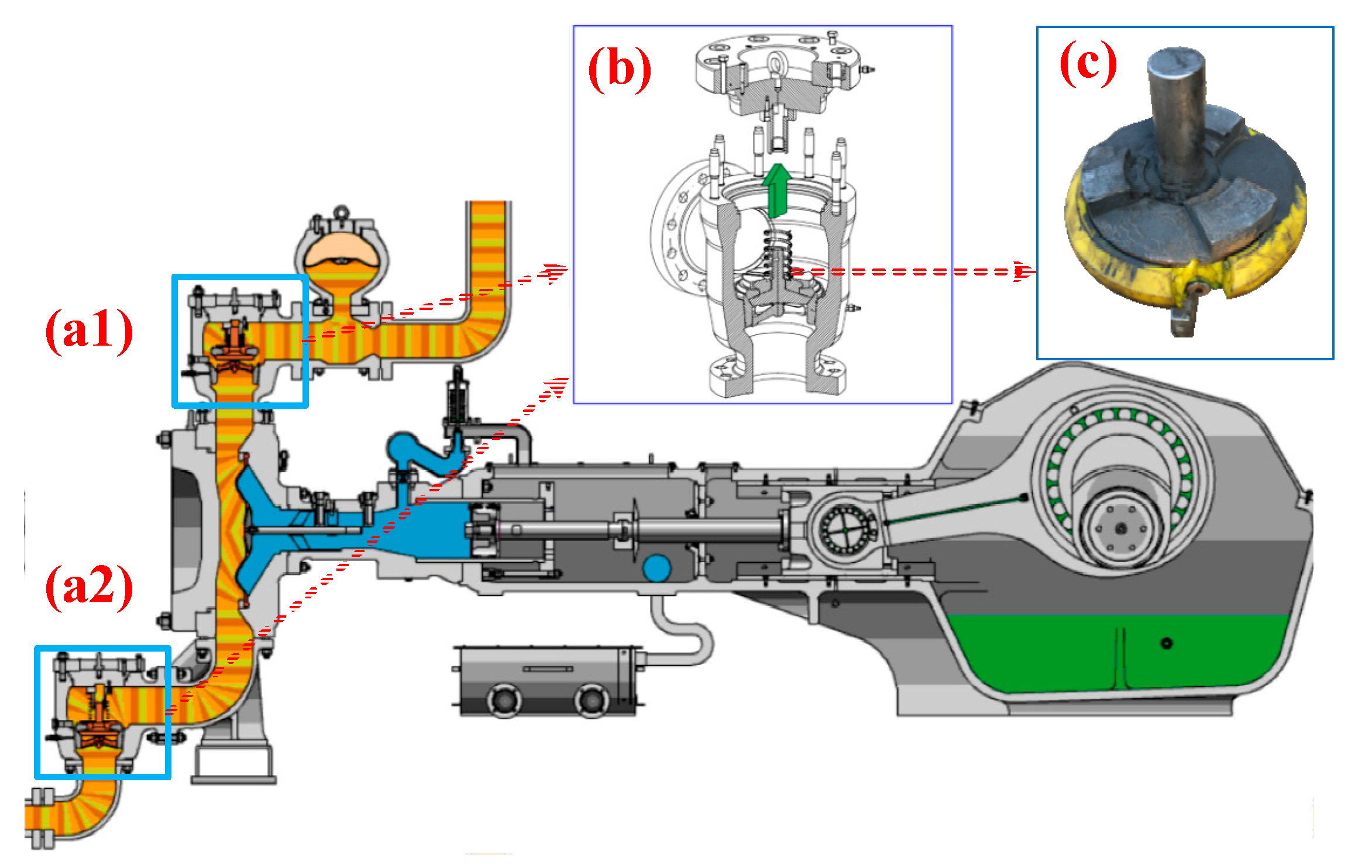
The experimental data come from the GEHO-TZPM2000 diaphragm pump (WEIR MINERALS NETHERLANDS B.V., EGTENRAYSEWEG 9 NL-5928 PH VENLO NETHERLANDS) of the DaHongShan slurry pipeline transportation system. The maximum pressure of the main pump is 24.4 MPa, the working pressure range is 18~21 MPa, the transmission elevation difference is 1520 m and the flow rate is 350 m²/h. The internal components of the GEHO-TZPM2000 diaphragm pump include three feed check valves and three discharge check valves. Figure 8(a1,a2) show a discharge check valve and a feed check valve respectively. The mechanical structure of the diaphragm pump check valve is shown in Figure 8b, and the spool spring forms a weakly damped oscillation system. When the diaphragm pump is running, the coordinated operation of the feed check valve and the discharge check valve makes the slurry flow smoothly. The valve core of the check valve moves back and forth in the valve chamber, the frequent contact between the valve core and the slurry often causes damage to the valve core of check valve, and Figure 8c shows a valve core that has been punctured. The sensor measuring point position and signal acquisition system are shown in Figure 9, and six PCB 352C33 sensors (PCB PIEZOTRONICS, Buffalo, NY, USA) are mounted on the shells of No. 1, No. 2, and No. 3 feed valves and No. 1, No. 2, and No. 3 discharge valves respectively. The vibration signal of the No. 1, No. 2, and No. 3 feed valves are collected through 0, 2, and 4 channels of the PXI-3342 acquisition card (Beijing Fanhua Hengxing Technology Co., Ltd, Beijing, China.), and the vibration signals of the No. 1, No. 2, and No. 3 discharge valves are collected through channels 1, 3, and 5, respectively. The sampling frequency is 2560 Hz and the data length is 76,800.

The vibration signal of the check valve is collected through a phased data acquisition scheme. The check valve is in a safe operation state within the first 500 h, so the vibration data is collected every 2 h to improve the data acquisition efficiency. The check valve may be in an early fault state from the 500th hour to the 1000th hour, so the vibration data is collected every 10 min. The check valve may be in a severe wear phase after the 1000th hour, so vibration data is collected every 2 min. Then, 421 time point samples are selected from all the time point samples obtained, and each time point sample contains 2048 data points. The sampling data is shown in Figure 10. Different from the sampling data of the bearing, the state degradation data of the check valve contains burrs and noise at any stage, and the change of amplitude is irregular. Therefore, it is more difficult to detect the fault state of the check valve compared with the bearing.

In order to verify the state tracking performance of the proposed SDE feature, it is compared with time domain, frequency domain, time-frequency domain features, fusion features and entropy features. For the check valve vibration signals from the first time point to the 421th time point, the SDE features of the vibration signals at each time point are extracted respectively, and an SDE degradation curve is obtained. Among them, the first 7680 data points of the vibration signal at each time point are used to extract the fault degradation features. Similarly, for the check valve vibration signals corresponding to 421 time points, their 16 time domain features (T1~T16), 13 frequency domain features (F1~F13), 8 wavelet packet energy features (TF1~TF8), 3 mixed domain fusion features based on PCA, LLE, and LLTSA, and 3 entropy features based on SE, PE, and DE can be obtained, and the state tracking performance of all the above degradation feature curves can be evaluated by the mixed evaluation index (MEI).

As shown in

Table 2. The evaluation results of check valve fault state detection.

Feature	Mon	Rob	Tre	MEI	Feature	Mon	Rob	Tre	MEI
T1	0.0380	0.8520	0.0652	0.2877	F7	0.0571	0.9479	0.3254	0.3780
T2	0.0285	0.8501	0.0620	0.2817	F8	0.0333	0.9745	0.3589	0.3808
T3 RMS	0.0142	0.8411	0.1026	0.2800	F9	0.0333	0.9621	0.2066	0.3466
T4	0.0380	0.8520	0.0652	0.2877	F10	0.0380	0.8982	0.3893	0.3663
T5	0.0428	0.6580	0.0841	0.2356	F11	0.0095	0.8498	0.3105	0.3218
T6 Kurt	0.0571	0.5694	0.0840	0.2162	F12	0.0190	0.7823	0.1837	0.2809
T7	0.0095	0.7583	0.5998	0.3522	F13	0.0047	0.8443	0.3905	0.3338
T8	0.0142	0.7584	0.5962	0.3539	TF1	0.0285	0.7802	0.6846	0.3952
T9	0.0190	0.6151	0.0824	0.2105	TF2	0.0238	0.7716	0.6425	0.3719
T10	0.0142	0.7518	0.0836	0.2494	TF3	0.0047	0.7035	0.4003	0.2935
T11	0.0047	0.9547	0.6221	0.4132	TF4	0.0047	0.7427	0.5321	0.3316
T12	0.0380	0.7902	0.6644	0.3889	TF5	0.0428	0.6275	0.4898	0.3076
T13	0.0095	0.7778	0.6722	0.3725	TF6	0.0047	0.6974	0.4431	0.3002
T14	0.0047	0.7746	0.6716	0.3691	TF7	0.0190	0.7107	0.3904	0.3008
T15	0.0142	0.8359	0.6561	0.3891	TF8	0.0047	0.7117	0.4510	0.3061
T16	0.0190	0.7838	0.6324	0.3711	PCA	0.0428	0.9920	0.0840	0.3358
F1	0.0142	0.8139	0.3309	0.3175	LLE	0.0071	0.9999	0.5083	0.4052
F2	0.0190	0.7601	0.0829	0.2541	LLTSA	0.0095	0.6520	0.1708	0.2345
F3	0.0047	0.9328	0.6328	0.4087	SE	0.0095	0.8861	0.3336	0.3373
F4	0.0142	0.9112	0.6350	0.4055	PE	0.0238	0.9742	0.4658	0.3973
F5	0.0761	0.9338	0.3794	0.3941	DE	0.0285	0.9581	0.5538	0.4125
F6	0.0285	0.8726	0.4408	0.3642	SDE	0.0666	0.9494	0.6001	0.4382

, the monotonicity index (Mon) 0.0666, robustness index (Rob) 0.9494 and trend index (Tre) 0.6001 of the SDE feature are close to the corresponding maximum 0.0761, 0.9999, and 0.6846, and the MEI 0.4382 of the SDE feature is the largest, which indicates that the SDE feature has the best state tracking performance. In addition, the MEIs of T11, DE, F3, and LLE features are 0.4132, 0.4125, 0.4087, and 0.4052, respectively, which indicates that these features can also achieve good degradation state characterization performance. In addition to SDE, DE, and LLE features, those features that can characterize the operating state of the bearing cannot characterize the operating state of the check valve effectively, such as RMS, SE, PE, F10, and F5. The results show that it is more difficult to track the operating state of the check valve, and the single feature is only sensitive to a specific degradation stage or a specific fault state. Although the fusion features such as PCA, LLE, and LLTSA can characterize the fault state information of machinery, these fusion features have strong relevance and redundancy. The MEI index of the 44 degradation features of the check valve is smaller than that of bearing, which indicates that the degradation process of check valve is more complex and the state tracking is more difficult. The reason is that the vibration signal of the check valve is affected by the slurry scouring and multi-part vibration and has nonlinear and non-stationary characteristics, and the traditional degradation features are not suitable for the fault state monitoring of the check valve.

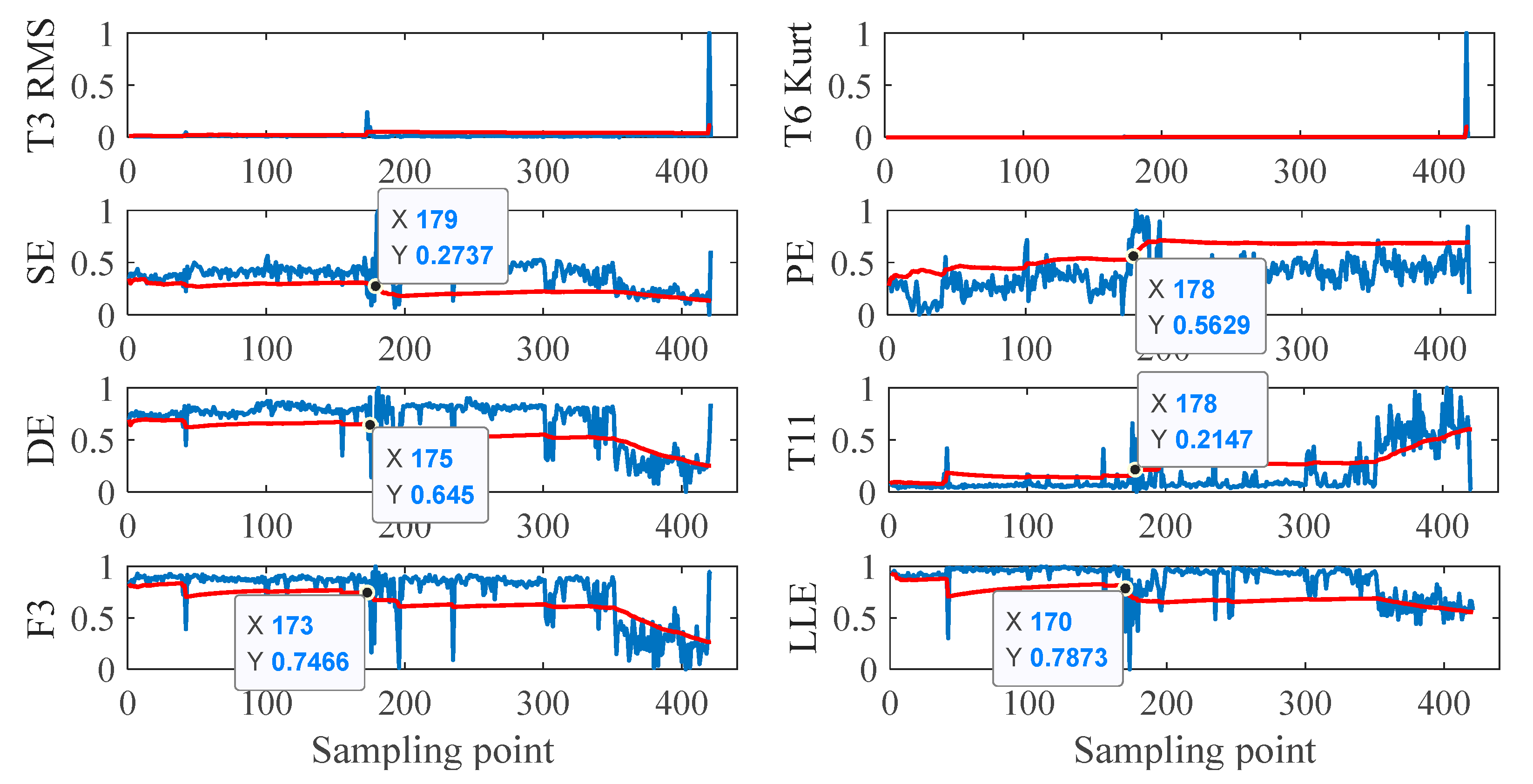
The RMS, Kurt, SE, PE, and DE features and their state warning lines are shown in Figure 11. In addition, Figure 11 also shows the T11, F3 and LLE feature curves with large MEI indexes. The RMS (MEI = 0.28), Kurt (MEI = 0.216), SE (MEI = 0.337), and PE (MEI = 0.397) features that can characterize the degradation state of the bearing cannot characterize the degradation state of the check valve, and these features can only detect the abnormal state at the 178th or 179th time point. The feature curves of DE, T11, F3, and LLE contain many burrs, and the phased variation of the curve is not obvious. In addition, the state warning line of these four features contains several turning points. Based on this, it can be determined that the fault warning point is roughly between the 170th time point and the 178th time point, and the check valve is in the severe wear phase between the 330th time point and the 421st time point. This is due to the complex structure of the diaphragm pump and the variability of influencing factors in the slurry transportation environment, which makes it difficult to track the fault state of the check valve.

The fault features of the check valve are not obvious in the slurry transportation environment. If the damage is not detected until it develops to a certain extent, the repair time will be insufficient and the repair cost may increase exponentially. Figure 12 shows the normalized SDE feature and smooth SDE feature of the check valve, and the corresponding state warning lines (red curve). As shown in Figure 12a, the SDE feature is close to 1 and the check valve is in a normal state from the first time point to the 169th time point. The SDE feature has a significant decline in stages from the 170th time point to the 326th time point, and the check valve may be in a state of slight wear. The decline of the SDE feature is more obvious from the 327th time point to the 421st time point, and the check valve may be in a state of severe wear. However, the SDE feature curve contains many burrs and fluctuations, which makes it difficult to determine the fault warning point through the state warning line, and the SDE feature can only detect the 170th time point as the state mutation point. Therefore, it is particularly necessary to track the state of check valve through the proposed smooth SDE. As shown in Figure 12b, the state warning line of smooth SDE can detect that the 168th time point is the fault warning point, and the 318th time point is the key state point. In addition, the smooth SDE feature can track the operation state of the check valve effectively. The tracking results show that the check valve is in a normal state from the first time point to the 168th time point, slightly worn from the 169th time point to the 318th time point, and seriously worn from the 319th time point to the 421st time point. Under the influence of noise and burrs, the smooth SDE feature and its state warning line can track the degradation state of the check valve effectively and detect the fault warning point earlier.

3.3. Comparison and Discussion

Through the two sets of experiments, the effectiveness and superiority of the proposed SDE and its adaptive state warning line have been proved. In order to further verify the superiority of the method proposed in this paper, the proposed SDE is also compared with the latest research results. Under the background of the same IMS bearing degradation experiment, the SDE proposed in this paper (Figure 7) can detect the fault warning point adaptively at the 525th time point. However, the energy moment entropy [22] proposed by Gao cannot detect the fault warning point until the 538th time point. Similarly, the oscillation based permutation entropy [13] proposed by Noman cannot detect the fault warning point until the 533th time point. The results show that the SDE proposed in this paper can detect the fault warning point of mechanical parts earlier and provide more response time for the repair and replacement of parts. Although the complex wavelet packet energy moment entropy [23] proposed by Shao can also detect fault warning point at the 525th time point, the determination of the fault warning point depends on manual experience and lacks an adaptive state warning line. In contrast, the method proposed in this paper can track and detect early fault warning points adaptively. In addition, compared with the latest research results, the proposed SDE has a high tracking efficiency, and the smoothness and effectiveness of the SDE tracking curve are significant. To sum up, the proposed fault state detection method based on SDE has outstanding effectiveness and superiority.

4. Conclusions

In this paper, a fault state detection and evaluation method based on SDE is proposed, which can track the degradation state of bearing and check valve and detect the operation state of mechanical parts at the current time. Through the analysis of the IMS bearing data in the laboratory environment and the check valve data in the industrial environment, the effectiveness of the proposed method is proved. By comparing the proposed SDE with single features, fusion feature and traditional entropy feature, the following conclusions can be drawn.

(1) In the condition monitoring of check valve and bearing, the MEI scores of SDE features are 0.4382 and 0.4717, respectively, and these two scores are much higher than those of single features, fusion features, and traditional entropy features. The results show that sliding window down-sampling improves the trend of degradation features, TANSIG mapping enhances the performance of SDE features to characterize degradation states, and the introduction of LOWESS improves the anti-interference performance of features. The SDE feature and its state warning line can effectively track the operation state of the check valve and determine the fault warning point earlier.

(2) The reason why the MEI scores of the 44 degradation features of the check valve is smaller than that of the 44 degradation features of the bearing is that the vibration signal of check valve in industrial environment is affected by factors such as slurry erosion and multi-part vibration. Even so, the proposed smooth SDE feature can still detect the degradation state of the check valve effectively.

(3) A new method for fault detection of mechanical parts is proposed in this paper, which can not only guide the formulation of maintenance and replacement plan, but also improve the operation safety of diaphragm pump and other equipment. Next, we will study the fault trend prediction methods and early fault diagnosis techniques.

References

1. Li, W.; Mckeown, A.; Yu, Z. Correction of cavitation with thermodynamic effect for a diaphragm pump in organic Rankine cycle systems. Energy Rep. 2020, 6, 2956–2972. [Google Scholar] [CrossRef]
2. Xiao, L.; Liu, Z.; Zhang, Y.; Zheng, Y.; Cheng, C. Degradation assessment of bearings with trend-reconstruct-based features selection and gated recurrent unit network. Measurement 2020, 165, 108064. [Google Scholar] [CrossRef]
3. Gao, S.; Zhang, S.; Zhang, Y.; Gao, Y. Operational reliability evaluation and prediction of rolling bearing based on isometric mapping and NoCuSa-LSSVM. Reliab. Eng. Syst. Saf. 2020, 201, 106968. [Google Scholar] [CrossRef]
4. Hua, Z.; Xiao, Y.; Cao, J. Misalignment Fault Prediction of Wind Turbines Based on Improved Artificial Fish Swarm Algorithm. Entropy 2021, 23, 692. [Google Scholar] [CrossRef] [PubMed]
5. Li, Z.; Zhang, X.; Kari, T.; Hu, W. Health Assessment and Remaining Useful Life Prediction of Wind Turbine High-Speed Shaft Bearings. Energies 2021, 14, 4612. [Google Scholar] [CrossRef]
6. Bilendo, F.; Badihi, H.; Lu, N.; Jiang, B. A data-driven prognostics method for explicit health index assessment and improved remaining useful life prediction of bearings. ISA Trans. 2021. [Google Scholar] [CrossRef] [PubMed]
7. He, M.; Zhou, Y.; Li, Y.; Wu, G.; Tang, G. Long short-term memory network with multi-resolution singular value decomposition for prediction of bearing performance degradation. Measurement 2020, 156, 107582. [Google Scholar] [CrossRef]
8. Ding, N.; Li, H.; Yin, Z.; Jiang, F. A novel method for journal bearing degradation evaluation and remaining useful life prediction under different working conditions. Measurement 2021, 177, 109273. [Google Scholar] [CrossRef]
9. Hu, M.; Wang, G.; Ma, K.; Cao, Z.; Yang, S. Bearing performance degradation assessment based on optimized EWT and CNN. Measurement 2021, 172, 108868. [Google Scholar] [CrossRef]
10. Shannon, C.E. A mathematical theory of communication. Mob. Comput. Commun. Rev. 2001, 5, 3–55. [Google Scholar] [CrossRef]
11. Qin, A.-S.; Mao, H.-L.; Hu, Q. Cross-domain fault diagnosis of rolling bearing using similar features-based transfer approach. Measurement 2021, 172, 108900. [Google Scholar] [CrossRef]
12. Kumar, P.S.; Kumaraswamidhas, L.; Laha, S. Selection of efficient degradation features for rolling element bearing prognosis using Gaussian Process Regression method. ISA Trans. 2021, 112, 386–401. [Google Scholar] [CrossRef] [PubMed]
13. Noman, K.; Wang, D.; Peng, Z.; He, Q. Oscillation based permutation entropy calculation as a dynamic nonlinear feature for health monitoring of rolling element bearing. Measurement 2021, 172, 108891. [Google Scholar] [CrossRef]
14. Minhas, A.S.; Kankar, P.; Kumar, N.; Singh, S. Bearing fault detection and recognition methodology based on weighted multiscale entropy approach. Mech. Syst. Signal Process. 2021, 147, 107073. [Google Scholar] [CrossRef]
15. Li, H.; Sun, J.; Ma, H.; Tian, Z.; Li, Y. A novel method based upon modified composite spectrum and relative entropy for degradation feature extraction of hydraulic pump. Mech. Syst. Signal Process. 2019, 114, 399–412. [Google Scholar] [CrossRef]
16. Mostafa, R.; Reza, A.M.; Hamed, A. Application of dispersion entropy to status characterization of rotary machines. J. Sound Vib. 2018, 438, 291–308. [Google Scholar]
17. Rostaghi, M.; Azami, H. Dispersion Entropy: A Measure for Time-Series Analysis. IEEE Signal Process. Lett. 2016, 23, 610–614. [Google Scholar] [CrossRef]
18. Zhang, B.; Zhang, S.; Li, W. Bearing performance degradation assessment using long short-term memory recurrent network. Comput. Ind. 2019, 106, 14–29. [Google Scholar] [CrossRef]
19. Azami, H.; Rostaghi, M.; Escudero, J. Refined composite multiscale dispersion entropy: A fast measure of complexity. IEEE Trans. Bio-Med. Eng. 2016, 99, 1–5. [Google Scholar]
20. Cleveland, W.S. LOWESS: A Program for Smoothing Scatterplots by Robust Locally Weighted Regression. Am. Stat. 1981, 35, 54. [Google Scholar] [CrossRef]
21. Duong, P.B.; Khan, A.S.; Shon, D.; Im, K. A Reliable Health Indicator for Fault Prognosis of Bearings. Sensors 2018, 18, 3740. [Google Scholar] [CrossRef] [PubMed] [Green Version]
22. Gao, Z.; Liu, Y.; Wang, Q.; Wang, J.; Luo, Y. Ensemble empirical mode decomposition energy moment entropy and enhanced long short-term memory for early fault prediction of bearing. Measurement 2021, 110417. [Google Scholar] [CrossRef]
23. Haidong, S.; Junsheng, C.; Hongkai, J.; Yu, Y.; Zhantao, W. Enhanced deep gated recurrent unit and complex wavelet packet energy moment entropy for early fault prognosis of bearing. Knowl. Based Syst. 2020, 188, 105022. [Google Scholar] [CrossRef]
Figure 1. The schematic diagram of sliding window and down−sampling.
Coatings 11 01536 g001
Figure 2. Comparison of mapping methods and classification of mapped data. (a) Comparison of different mapping methods; (b) data classification after TANSIG mapping.
Coatings 11 01536 g002
Figure 3. Flow chart of fault state detection and evaluation method.
Coatings 11 01536 g003
Figure 4. Illustration of the bearing experiment platform. (a) Bearing test rig; (b) sensor placement illustration; (c) outer race defect of set number 2.
Coatings 11 01536 g004
Figure 5. Bearing sampling signal.
Coatings 11 01536 g005
Figure 6. Bearing fault feature curve (blue curve) and state warning line (red curve).
Coatings 11 01536 g006
Figure 7. SDE and Smooth SDE curve (blue curve) and corresponding state warning line (red curve). (a) SDE; (b) smooth SDE.
Coatings 11 01536 g007
Figure 8. The structure of the diaphragm pump and check valve. (a1) discharge check valve; (a2) feed check valve; (b) structure of check valve; (c) a valve core that has been punctured.
Coatings 11 01536 g008
Figure 9. Sensor measuring point, acquisition platform and fault check valve. (a) Inlet valve measuring point; (b) Outlet valve measuring point; (c) Data acquisition device; (d) Stuck valve fault; (e) Wear fault; (f) Worn valve seat; (g) Replaced check valve.
Coatings 11 01536 g009
Figure 10. Check valve sampling signal.
Coatings 11 01536 g010
Figure 11. Check valve fault feature curve (blue curve) and status warning line (red curve).
Coatings 11 01536 g011
Figure 12. SDE and SDE feature curve (blue curve) and corresponding state warning line (red curve). (a) SDE; (b) smooth SDE.
Coatings 11 01536 g012