
Machine Learning Model to Map Tribocorrosion Regimes in Feature Space


Department of Mechanical Engineering, University of Nevada, Reno, NV 89557, USA
Coatings 2021, 11(4), 450; https://doi.org/10.3390/coatings11040450
Submission received: 3 March 2021
/
Revised: 10 April 2021
/
Accepted: 13 April 2021
/
Published: 14 April 2021
(This article belongs to the Special Issue Tribology in Material Forming)
Abstract
:Degradation by wear and corrosion are frequently encountered in a variety of tribosystems, including materials and tools in forming operations. The combined effect of wear and corrosion, known as tribocorrosion, can result in accelerated material degradation. Interfacial conditions can affect this degradation. Tribocorrosion maps serve the purpose of identifying operating conditions at the interface for an acceptable rate of degradation. This paper proposes a machine learning-based approach to generate tribocorrosion maps, which can be used to predict tribosystem performance. Two tribocorrosion datasets from the published literature are used. The materials have been chosen based on the wide availability of their tribocorrosion data in the literature. First, unsupervised machine learning is used to identify and label clusters from tribocorrosion data. The identified clusters are then used to train a support vector classification model. The trained support vector machine is used to generate tribocorrosion maps. The generated maps are compared with those from the literature. The general approach can be applied to create tribocorrosion maps of materials widely used in material forming.
1. Introduction
The development and implementation of predictive models from experimental data using machine learning (ML) has been an active research topic in material science and engineering. In ML, a computer program based on an algorithm learns from historical data to improve a performance metric. The selection of the algorithm and metric depend on the specific data and problem at hand. The commonly used ML algorithms can be divided into regression, probability estimation, classification and clustering [1]. Recently, ML tools have been used in tribology to build predictive models for friction coefficient [2,3], wear rate [4] and wear volume [5], to design lubricants [6,7,8] and functional materials [9], for tribocorrosion [10] and surface roughness [11] modeling, for wear particle classification [12], in corrosion modeling [13,14,15,16,17,18,19], and in medical implant classification [20].
Tribocorrosion, which is the combined effect of wear and corrosion, is often undesirable and can accelerate material degradation. It is frequently encountered where surfaces are in contact with each other in a corrosive environment. Interfacial conditions such as materials, lubrication, normal load, type of contact (sliding, fretting, rolling, impact), relative speed, surface topography, temperature, humidity and pH can affect the degradation process [21]. This phenomenon is relevant to a range of industries such as material forming and machining [22,23,24,25,26], mining and energy [27,28,29], healthcare [30], and transportation [31]. The total mass change by tribocorrosion (Kwc) can be explained using the analysis in [32] as
where Kw is the total mass of material removed due to wear, Kc is the total mass of material removed due to corrosion. Kw is Kwo + ∆Kw, where Kwo is the mass loss by wear in the absence of corrosion, and ∆Kw is the synergistic effect of corrosion on wear. Kc is Kco + ∆Kc, where Kco is the mass loss by corrosion in the absence of wear, and ∆Kc is the additive effect (enhancement) of corrosion due to wear. These terms can be determined experimentally and used to characterize the dominant degenerative mechanism for the tribosystem. Tribocorrosion regimes [33] are defined based on the ratio Kc/Kw as follows:
Tribocorrosion mechanism maps and synergy maps illustrate these regimes as functions of interfacial conditions such as normal load, sliding speed and pH. These maps are helpful to optimize material forming processes, identify conditions of minimal degradation, improve tool life, and design functional materials and coatings [34].
The standard approach to create tribocorrosion maps involves extensive experiments to generate data, determine the regimes and create graphical illustrations. Machine learning can be used to quickly and automatically create accurate predictive models from the experimental data. Although ML tools are widely used in tribology, no previous studies have dealt with identifying clusters and creating tribocorrosion maps using ML tools. This study uses both unsupervised and supervised learning techniques to make predictive models for tribocorrosion and to generate maps. The two datasets used to create the models are from published tribocorrosion studies. The materials used in these studies are the alloys Ti–25Nb–3Mo–3Zr–2Sn and Co–Cr. These have been chosen because their tribocorrosion data are widely available in the literature.
The titanium alloy has mechanical properties that make it suitable for a wide range of applications. It has a yield strength in the range of 440–500 MPa, elastic modulus in the range of 50–80 GPa, and ultimate tensile strength in the range of 708–715 MPa [35]. The corrosion potential of −0.51 V and the corrosion current density of 0.13 μA/cm2 were reported for the alloy in phosphate-buffered solution simulating physiological environment [36]. Their high strength-to-weight ratio, low modulus of elasticity, corrosion resistance, and biocompatibility make them ideal for biomedical implants.
Co–Cr alloys are also widely used in biomedical implants due to their high specific strength, hardness, corrosion resistance, and biocompatibility. Their tensile strength is in the range of 145–270 MPa and hardness in the range of 550–800 MPa [37]. The corrosion potential and corrosion current density of Co–Cr in artificial saliva is about −0.45 V and 0.16 μA/cm2 [38].
This study presents an ML-based general methodology to create tribocorrosion maps. The same process can be applied to create similar maps of materials widely used in material forming. The ML methodology is discussed in the following section.
2. Methodology
The predictive model is developed in two parts. The first part involves identifying clusters in tribocorrosion experimental data using the K-Means clustering technique. The second part involves training a support vector classifier using the data and the cluster labels. The support vectors can then be used to draw wear-corrosion mechanism, synergy, and wastage maps. The schematic in Figure 1 shows an overview of the proposed methodology. Two experimental datasets from the published literature are used in this study. The materials in these studies, albeit related to medical implants, are the subject of several tribocorrosion studies. Therefore, their relatively large volume of experimental tribocorrosion data is widely available. Note that the volume of the dataset is decisive in effectively training an ML algorithm.
Wang et al. [39] studied the tribocorrosion of Ti–25Nb–3Mo–3Zr–2Sn alloy in a simulated Hank’s solution at different loads and abrasive silicon carbide concentrations. The data from Wang et al. are labelled Dataset 1 (see Supplementary Materials, Table S1). Dataset 2 (see Supplementary Materials, Table S2) was collected from the work of Stack et al. [40]. That study focused on the tribocorrosion of Co–Cr in Ringer’s solution mixed with silicon carbide particles at different loads and applied potentials.
It is essential to understand the degradation and predict the lifecycle of the materials under various conditions, both of which can possibly be done with ML. The data were standardized by removing the mean and scaling to unit variance before training the model. The models were developed using the open source ML package scikit-learn [41].
2.1. Unsupervised Learning
Clustering is a multivariate statistical technique used to group data into clusters based on their underlying structure. A commonly used technique is K-means clustering. The number of clusters (K) and the starting centroids are provided as input parameters. This is followed by an iterative process of assigning the data points to each cluster based on their Euclidean squared distance to the corresponding centroid, and recalculating the centroids, until the centroids can no longer be adjusted.
2.2. Supervised Learning
Support vector machines (SVMs) [44] are supervised ML algorithms that can be used for classification and regression [45]. SVMs use kernel functions to map datapoints from an input space to a high dimensional feature space to establish linear decision boundaries (hyper planes). These boundaries become nonlinear when transformed back to original input space, thus making non-linear classification possible. The datapoints closest to the hyperplane are called support vectors. Four basic kernel functions k(xi,xj) are linear (Equation (6)), polynomial (Equation (7)), radial basis function (RBF) (Equation (8)) and sigmoid (Equation (9)). The hyperparameters γ, r, and d associated with the SVMs are generally tuned using cross-validation or grid search [46]:
The labelled datasets obtained after clustering is used to train SVM classification models. Since SVMs are designed for binary classification, different strategies can be adopted based on the multiclass classification problem at hand [47].
3. Results and Discussion
3.1. Identifying the Clusters
Clustering was done for a range of K values based on the data, and the resulting within-cluster sum of squares (WCSS) was obtained. The red lines in Figure 2a,b show the WCSS for datasets 1 and 2, respectively. An elbow point in the WCSS graph typically signifies the optimal K value. The elbow can be observed at K = 3 in Figure 2a. However, the elbow in Figure 2b is not obvious. Further analysis was done by calculating the silhouette coefficients. The blue lines in Figure 2a,b show the silhouette coefficients for a range of K values for datasets 1 and 2, respectively. The best value of K is where the silhouette coefficient is maximum, which is equal to 3 for both the datasets.
It is worth noting that among the two methods discussed above to determine the optimal K, the elbow method can be ambiguous when the data are not very clustered. In such cases, the WCSS curve may not have a sharp elbow. Silhouette coefficient, on the other hand, is a value between +1 and −1, with values closer to the upper bound indicating appropriate clustering. Thus, a silhouette coefficient is a more robust metric to determine K.
The two datasets were clustered and labelled using K-means clustering with K = 3. The three clusters in dataset 1 can clearly be distinguished on a Kw vs. Kc plot as shown in Figure 3a. The single datapoint that forms a distinct cluster is identified as the corrosion–wear cluster, as it has a high Kc compared to Kw. The other two clusters are closer to the Kw axis, denoting wear-corrosion synergy. The cluster near the origin is labelled as the low wear-corrosion synergy cluster, and the cluster in the lower right-hand corner is labelled as the high wear-corrosion synergy cluster.
Similarly, the three clusters in dataset 2 can be clearly identified on a Kc vs. Kw plot as shown in Figure 4a. The cluster with the very small values of Kc, and large values of Kw can be identified as having wear as the predominant degradation mechanism. The cluster in the top left-hand corner with similar values of Kc and Kw can be identified as having corrosion-wear synergy. The third cluster, approximately in the center of the plot, is classed as having wear–corrosion synergy. This classification is similar to the results obtained in the source [40].
3.2. Tribocorrosion Maps
Since the two datasets under consideration have three clusters each, a one-vs.-one strategy was used to train the SVM and perform classification. The clusters in dataset 1 were labelled 0, 1 and 2. The features used were abrasive concentration (g/cm3) and normal load (N). A polynomial kernel function was chosen to map the datapoints to a higher dimensional space. Values for the hyperparameters in Equation (7) were as follows: kernel parameter γ = 2, penalty parameter = 10, degree d = 2 and r = 0. The model was trained on the labelled dataset. The tribocorrosion map (Figure 3b) of the feature space—abrasive particle concentration vs. normal load—was generated by prediction using the trained model. The map shows the three previously identified clusters. From the map, the major degradation mechanism is identified as wear-induced corrosion, which is similar to the results obtained by [39]. Corrosion-induced wear is the degradation mechanism for a small segment of the operating conditions.
Similarly, the clusters in dataset 2 were labelled as 0, 1 and 2. The features used were potential (V) and normal load (N). RBF kernel (Equation (8)) was used to map the dataset 2 to a higher dimensional space. The model was trained on the labelled dataset with hyperparameter γ = 7 and the penalty parameter as 10. The tribocorrosion map obtained by predicting using the trained model on the feature space is shown in Figure 4b. The three degradation mechanisms—wear, wear–corrosion, and corrosion-wear—are mapped on the potential vs. normal load graph. The wear-corrosion cluster, as identified in Figure 4a, covers most of the area in the tribocorrosion map. Wear is the dominant degradation mechanism in the potential range from −0.5 to −0.3 V. Corrosion-induced wear dominates in the region near 0 V potential.
Thus, the relationship between competing material degradation mechanisms is determined for the two tribosystems under consideration. From Figure 3b and Figure 4b, the dominant degradation mechanism for a given set of features can be identified. With this knowledge, acceptable material loss rate can potentially be achieved by maintaining the interfacial conditions within certain bounds identified from the maps. Based on the availability of empirical data, maps can be generated in any desired feature space. Note that Figure 3b is mapped on load vs. abrasive concentration, while Figure 4b is mapped on load vs. potential.
Although the data used in this study are for specific materials, the method proposed is relevant to mapping tribocorrosion in a range of tribosystems. The maps provide an overall framework in which we can analyze the relationship between the variables, their correlation to material degradation rate, and the dominant wastage mechanisms. Potential applications include prediction of degradation mechanism and wastage rate, material selection, and lifecycle estimation of tools, material processing equipment, automotive and marine machine components.
In this study, the performance of the models was not evaluated using test and validation datasets due to limited sample sizes. It is important to note that test and validation datasets are necessary to prevent over-fitting the models. In future work, more robust ML predictive models will be created using a larger training dataset.
4. Conclusions
A machine learning-based approach is proposed to generate tribocorrosion maps. First, tribocorrosion experimental data are clustered and labelled based on their underlying structure. The labelled datasets are used to train SVM classification models, with the labels being the targets. Since problem is non-linear, RBF and polynomial kernels are used to map the data and establish the decision boundaries. The trained models are used to predict the targets on the feature space to generate the tribocorrosion maps. The proposed methodology to create tribocorrosion maps is relevant to any tribocorrosion system. Thus, it can find applications such as optimizing the material forming processes, material selection, identifying degradation mechanisms, lifecycle estimation, and improving tool life.
Supplementary Materials
The following are available online at https://www.mdpi.com/article/10.3390/coatings11040450/s1, Table S1: Dataset 1; Table S2: Dataset 2.
Funding
This research received no external funding.
Institutional Review Board Statement
Not applicable.
Informed Consent Statement
Not applicable.
Data Availability Statement
Data are included in the Supplementary Materials.
Conflicts of Interest
The author declares no conflict of interest.
References
- Liu, Y.; Zhao, T.; Ju, W.; Shi, S. Materials discovery and design using machine learning. J. Mater. 2017, 3, 159–177. [Google Scholar] [CrossRef]
- Xie, H.; Wang, Z.; Qin, N.; Du, W.; Qian, L. Prediction of Friction Coefficients During Scratch Based on an Integrated Finite Element and Artificial Neural Network Method. J. Tribol. 2020, 142, 1–25. [Google Scholar] [CrossRef]
- Gyurova, L.A.; Friedrich, K. Artificial neural networks for predicting sliding friction and wear properties of polyphenylene sulfide composites. Tribol. Int. 2011, 44, 603–609. [Google Scholar] [CrossRef]
- Argatov, I.I.; Chai, Y.S. An artificial neural network supported regression model for wear rate. Tribol. Int. 2019, 138, 211–214. [Google Scholar] [CrossRef]
- Velten, K.; Reinicke, R.; Friedrich, K. Wear volume prediction with artificial neural networks. Tribol. Int. 2000, 33, 731–736. [Google Scholar] [CrossRef]
- Bhaumik, S.; Pathak, S.D.; Dey, S.; Datta, S. Artificial intelligence based design of multiple friction modifiers dispersed castor oil and evaluating its tribological properties. Tribol. Int. 2019, 140, 105813. [Google Scholar] [CrossRef]
- Rashmi, W.; Osama, M.; Khalid, M.; Rasheed, A.K.; Bhaumik, S.; Wong, W.Y.; Datta, S.; TCSM, G. Tribological performance of nanographite-based metalworking fluid and parametric investigation using artificial neural network. Int. J. Adv. Manuf. Technol. 2019, 104, 359–374. [Google Scholar] [CrossRef]
- Humelnicu, C.; Ciortan, S.; Amortila, V. Artificial Neural Network-Based Analysis of the Tribological Behavior of Vegetable Oil–Diesel Fuel Mixtures. Lubricants 2019, 7, 32. [Google Scholar] [CrossRef] [Green Version]
- Vinoth, A.; Datta, S. Design of the ultrahigh molecular weight polyethylene composites with multiple nanoparticles: An artificial intelligence approach. J. Compos. Mater. 2019, 54, 179–192. [Google Scholar] [CrossRef]
- Pai, P.S.; Mathew, M.T.; Stack, M.M.; Rocha, L.A. Some thoughts on neural network modelling of microabrasion–corrosion processes. Tribol. Int. 2008, 41, 672–681. [Google Scholar] [CrossRef] [Green Version]
- Buj-Corral, I.; Sivatte-Adroer, M.; Llanas-Parra, X. Adaptive indirect neural network model for roughness in honing processes. Tribol. Int. 2020, 141, 105891. [Google Scholar] [CrossRef]
- Peng, Y.; Cai, J.; Wu, T.; Cao, G.; Kwok, N.; Zhou, S.; Peng, Z. A hybrid convolutional neural network for intelligent wear particle classification. Tribol. Int. 2019, 138, 166–173. [Google Scholar] [CrossRef]
- Kamrunnahar, M.; Urquidi-Macdonald, M. Prediction of corrosion behavior using neural network as a data mining tool. Corros. Sci. 2010, 52, 669–677. [Google Scholar] [CrossRef]
- Mareci, D.; Suditu, G.D.; Chelariu, R.; Trincă, L.C.; Curteanu, S. Prediction of corrosion resistance of some dental metallic materials applying artificial neural networks. Mater. Corros. 2016, 67, 1213–1219. [Google Scholar] [CrossRef]
- Jiménez-Come, M.J.; Turias, I.J.; Ruiz-Aguilar, J.J.; Trujillo, F.J. Characterization of pitting corrosion of stainless steel using artificial neural networks. Mater. Corros. 2015, 66, 1084–1091. [Google Scholar] [CrossRef] [Green Version]
- Mareci, D.; Dragoi, E.-N.; Bolat, G.; Chelariu, R.; Gordin, D.; Curteanu, S. Modelling the influence of pH, fluoride, and caffeine on the corrosion resistance of TiMo alloys by artificial neural networks developed with differential evolution algorithm. Mater. Corros. 2015, 66, 982–994. [Google Scholar] [CrossRef]
- Chelariu, R.; Suditu, G.D.; Mareci, D.; Bolat, G.; Cimpoesu, N.; Leon, F.; Curteanu, S. Prediction of Corrosion Resistance of Some Dental Metallic Materials with an Adaptive Regression Model. JOM 2015, 67, 767–774. [Google Scholar] [CrossRef]
- Xu, K.; Luxmoore, A.R.; Deravi, F. Comparison of shape features for the classification of wear particles. Eng. Appl. Artif. Intell. 1997, 10, 485–493. [Google Scholar] [CrossRef]
- Chou, J.-S.; Ngo, N.-T.; Chong, W.K. The use of artificial intelligence combiners for modeling steel pitting risk and corrosion rate. Eng. Appl. Artif. Intell. 2017, 65, 471–483. [Google Scholar] [CrossRef]
- Yılmaz, A. Shoulder Implant Manufacturer Detection by Using Deep Learning: Proposed Channel Selection Layer. Coatings 2021, 11, 346. [Google Scholar] [CrossRef]
- Landolt, D. Electrochemical and materials aspects of tribocorrosion systems. J. Phys. D Appl. Phys. 2006, 39, 3121–3127. [Google Scholar] [CrossRef]
- Richard, C. 19—Tribocorrosion at elevated temperatures in the metal working industry. In Woodhead Publishing Series in Metals and Surface Engineering; Landolt, D., Mischler, S., Eds.; Woodhead Publishing: Cambridge, UK, 2011; pp. 517–536. ISBN 978-1-84569-966-6. [Google Scholar]
- Bai, H.-D.; Zheng, B.-C.; Li, W.; Tu, X.-H. Failure analysis of ring die of a feed pellet machine. China Foundry 2020, 17, 167–172. [Google Scholar] [CrossRef]
- Behrens, B.-A.; Brunotte, K.; Wester, H.; Rothgänger, M.; Müller, F. Multi-Layer Wear and Tool Life Calculation for Forging Applications Considering Dynamical Hardness Modeling and Nitrided Layer Degradation. Materials 2020, 14, 104. [Google Scholar] [CrossRef]
- Karakaş, M.S. Tribocorrosion behavior of surface-modified AISI D2 steel. Surf. Coat. Technol. 2020, 394, 125884. [Google Scholar] [CrossRef]
- Zavieh, A.H.; Espallargas, N. Effect of 4-point bending and normal load on the tribocorrosion-fatigue (multi-degradation) of stainless steels. Tribol. Int. 2016, 99, 96–106. [Google Scholar] [CrossRef]
- Kasar, A.K.; Siddaiah, A.; Ramachandran, R.; Menezes, P.L. Tribocorrosion Performance of Tool Steel for Rock Drilling Process. J. Bio. Tribo-Corros. 2019, 5, 44. [Google Scholar] [CrossRef]
- Wood, R.J.K.; Herd, S.; Thakare, M.R. A critical review of the tribocorrosion of cemented and thermal sprayed tungsten carbide. Tribol. Int. 2018, 119, 491–509. [Google Scholar] [CrossRef]
- Kowalski, M.; Stachowiak, A. Tribocorrosion Performance of Cr/CrN Hybrid Layer as a Coating for Machine Components Used in a Chloride Ions Environment. Coatings 2021, 11, 242. [Google Scholar] [CrossRef]
- Rasool, G.; El Shafei, Y.; Stack, M.M. Mapping Tribo-Corrosion Behaviour of TI-6AL-4V Eli in Laboratory Simulated Hip Joint Environments. Lubricants 2020, 8, 69. [Google Scholar] [CrossRef]
- Siddaiah, A.; Khan, Z.A.; Ramachandran, R.; Menezes, P.L. Performance Analysis of Retrofitted Tribo-Corrosion Test Rig for Monitoring in Situ Oil Conditions. Materials 2017, 10, 1145. [Google Scholar] [CrossRef] [Green Version]
- Yue, Z.; Zhou, P.; Shi, J. Some Factors Influencing Corrosion-Erosion Performance of Materials. In Proceedings of the Wear of Materials, Houston, TX, USA, 5 April 1987; Luedema, K.C., Ed.; ASME: New York, NY, USA, 1987; pp. 763–770. [Google Scholar]
- Stack, M.M.; Zhou, S.; Newman, R.C. Effects of particle velocity and applied potential on erosion of mild steel in carbonate/bicarbonate slurry. Mater. Sci. Technol. 1996, 12, 261–268. [Google Scholar] [CrossRef]
- Wood, R.J.K. Tribo-corrosion of coatings: A review. J. Phys. D Appl. Phys. 2007, 40, 5502–5521. [Google Scholar] [CrossRef]
- Kent, D.; Wang, G.; Yu, Z.; Dargusch, M.S. Pseudoelastic behaviour of a β Ti–25Nb–3Zr–3Mo–2Sn alloy. Mater. Sci. Eng. A 2010, 527, 2246–2252. [Google Scholar] [CrossRef]
- Huang, W.; Wang, Z.; Liu, C.; Yu, Y. Wear and Electrochemical Corrosion Behavior of Biomedical Ti–25Nb–3Mo–3Zr–2Sn Alloy in Simulated Physiological Solutions. J. Bio. Tribo-Corros. 2015, 1, 1–10. [Google Scholar] [CrossRef] [Green Version]
- Sahoo, P.; Das, S.K.; Davim, J.P. Tribology of materials for biomedical applications. In Mechanical Behaviour of Biomaterials; Davim, J.P., Ed.; Woodhead Publishing: Cambridge, UK, 2019; pp. 1–45. [Google Scholar]
- Qiu, J.; Yu, W.-Q.; Zhang, F.-Q.; Smales, R.J.; Zhang, Y.-L.; Lu, C.-H. Corrosion behaviour and surface analysis of a Co-Cr and two Ni-Cr dental alloys before and after simulated porcelain firing. Eur. J. Oral Sci. 2011, 119, 93–101. [Google Scholar] [CrossRef] [PubMed]
- Wang, Z.; Li, Y.; Huang, W.; Chen, X.; He, H. Micro-abrasion–corrosion behaviour of a biomedical Ti–25Nb–3Mo–3Zr–2Sn alloy in simulated physiological fluid. J. Mech. Behav. Biomed. Mater. 2016, 63, 361–374. [Google Scholar] [CrossRef] [PubMed]
- Stack, M.M.; Rodling, J.; Mathew, M.T.; Jawan, H.; Huang, W.; Park, G.; Hodge, C. Micro-abrasion–corrosion of a Co–Cr/UHMWPE couple in Ringer’s solution: An approach to construction of mechanism and synergism maps for application to bio-implants. Wear 2010, 269, 376–382. [Google Scholar] [CrossRef] [Green Version]
- Pedregosa, F.; Varoquaux, G.; Gramfort, A.; Michel, V.; Thirion, B.; Grisel, O.; Blondel, M.; Prettenhofer, P.; Weiss, R.; Dubourg, V.; et al. Scikit-learn: Machine Learning in Python. J. Mach. Learn. Res. 2011, 12, 2825–2830. [Google Scholar]
- Milligan, G.W.; Cooper, M.C. An examination of procedures for determining the number of clusters in a data set. Psychometirka 1985, 50, 159–179. [Google Scholar] [CrossRef]
- Rousseeuw, P.J. Silhouettes: A graphical aid to the interpretation and validation of cluster analysis. J. Comput. Appl. Math. 1987, 20, 53–65. [Google Scholar] [CrossRef] [Green Version]
- Cortes, C.; Vapnik, V. Support-vector networks. Mach. Learn. 1995, 20, 273–297. [Google Scholar] [CrossRef]
- Naganna, S.R.; Deka, P.C. Support vector machine applications in the field of hydrology: A review. Appl. Soft Comput. 2014, 19, 372–386. [Google Scholar] [CrossRef]
- Hsu, C.-W.; Chang, C.-C.; Lin, C.-J. A Practical Guide to Support. Vector Classification. Available online: https://www.csie.ntu.edu.tw/~cjlin/papers/guide/guide.pdf (accessed on 15 December 2020).
- Brownlee, J. How to Use One-vs-Rest and One-vs-One for Multi-Class Classification. Available online: https://machinelearningmastery.com/one-vs-rest-and-one-vs-one-for-multi-class-classification/ (accessed on 10 January 2021).
Figure 1.
An overview of the methodology for creating tribocorrosion maps.

Figure 2.
Metrics to determine the optimum number of clusters for (a) dataset 1 and (b) dataset 2. Within-cluster sum of squares (WCSS) is denoted by the red circles and dashed line. Silhouette coefficients are denoted by blue squares and solid line.
Figure 2.
Metrics to determine the optimum number of clusters for (a) dataset 1 and (b) dataset 2. Within-cluster sum of squares (WCSS) is denoted by the red circles and dashed line. Silhouette coefficients are denoted by blue squares and solid line.

Figure 3.
(a) Three clusters in dataset 1 identified using K-means clustering; and (b) the tribocorrosion mechanism map using support vector machines (SVMs) for the titanium alloy.
Figure 3.
(a) Three clusters in dataset 1 identified using K-means clustering; and (b) the tribocorrosion mechanism map using support vector machines (SVMs) for the titanium alloy.
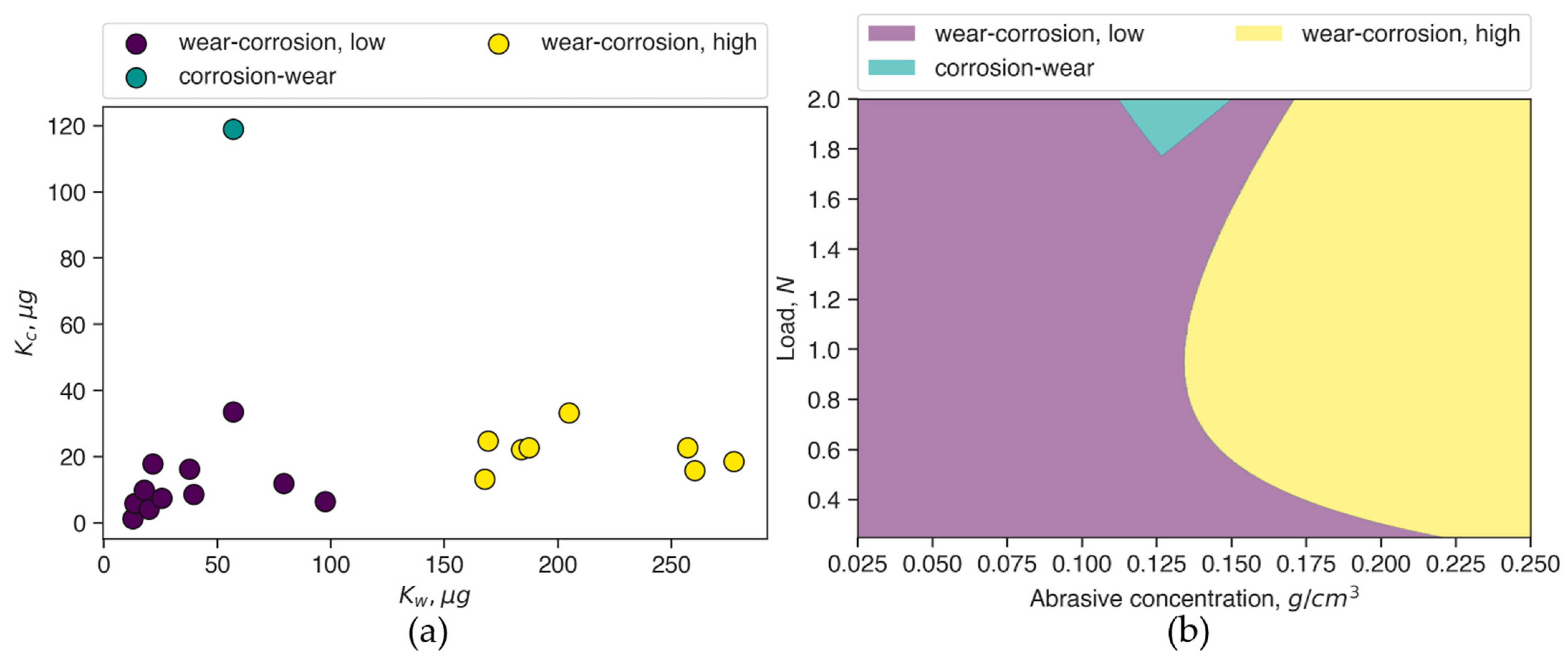
Figure 4.
(a) Three clusters in dataset 2 identified using K-means clustering; and (b) the tribocorrosion mechanism map of Co–Cr generated using SVM.
Figure 4.
(a) Three clusters in dataset 2 identified using K-means clustering; and (b) the tribocorrosion mechanism map of Co–Cr generated using SVM.

Publisher’s Note: MDPI stays neutral with regard to jurisdictional claims in published maps and institutional affiliations. |
© 2021 by the author. Licensee MDPI, Basel, Switzerland. This article is an open access article distributed under the terms and conditions of the Creative Commons Attribution (CC BY) license (https://creativecommons.org/licenses/by/4.0/).
Share and Cite
MDPI and ACS Style
Ramachandran, R. Machine Learning Model to Map Tribocorrosion Regimes in Feature Space. Coatings 2021, 11, 450. https://doi.org/10.3390/coatings11040450
AMA Style
Ramachandran R. Machine Learning Model to Map Tribocorrosion Regimes in Feature Space. Coatings. 2021; 11(4):450. https://doi.org/10.3390/coatings11040450
Chicago/Turabian StyleRamachandran, Rahul. 2021. "Machine Learning Model to Map Tribocorrosion Regimes in Feature Space" Coatings 11, no. 4: 450. https://doi.org/10.3390/coatings11040450
Note that from the first issue of 2016, this journal uses article numbers instead of page numbers. See further details here.