Multi-Objective Optimization of MIG Welding and Preheat Parameters for 6061-T6 Al Alloy T-Joints Using Artificial Neural Networks Based on FEM

Abstract

To control the welding residual stress and deformation of metal inert gas (MIG) welding, the influence of welding process parameters and preheat parameters (welding speed, heat input, preheat temperature, and preheat area) is discussed, and a prediction model is established to select the optimal combination of process parameters. Thermomechanical numerical analysis was performed to obtain the residual welding deformation and stress according to a 100 × 150 × 50 × 4 mm aluminum alloy 6061-T6 T-joint. Owing to the complexity of the welding process, an optimal Latin hypercube sampling (OLHS) method was adopted for sampling with uniformity and stratification. Analysis of variance (ANOVA) was used to find the influence degree of welding speed (7.5–9 mm/s), heat input (1500–1700 W), preheat temperature (80–125 °C), and preheat area (12–36 mm). The range of research parameters are according to the material, welding method, thickness of the welding plate, and welding procedure specification. Artificial neural network (ANN) and multi-objective particle swarm optimization (MOPSO) was combined to find the effective parameters to minimize welding deformation and stress. The results showed that preheat temperature and welding speed had the greatest effect on the minimization of welding residual deformation and stress, followed by the preheat area, respectively. The Pareto front was obtained by using the MOPSO algorithm with ε-dominance. The welding residual deformation and stress are the minimum at the same time, when the welding parameters are selected as preheating temperature 85 °C and preheating area 12 mm, welding speed is 8.8 mm/s and heat input is 1535 W, respectively. The optimization results were validated by the finite element (FE) method. The error between the FE results and the Pareto optimal compromise solutions is less than 12.5%. The optimum solutions in the Pareto front can be chosen by designers according to actual demand.

1. Introduction

With the rapid development of rail vehicles in China in recent years, an increasing number of high requirements have been put forward for the materials used in railway vehicles [1]. Among different lightweight materials, aluminum alloys possess an excellent strength-to-weight ratio and are extensively used in subways, intercity trains, and high-speed electric multiple units (EMU) [2,3,4]. However, due to the high linear expansion coefficient of 6061-T6, a study of methods to reduce the welding residual stress and deformation is urgently needed [5,6].

Many scholars have chosen to study and optimize the welding process parameters to improve the welding qualities and to reduce the welding residual deformation and residual tensile stress [7,8]. Kumar [9] studied the effects of MIG welding process parameters such as current, voltage, and preheat temperature and optimized them using gray-based Taguchi methodology. The influence of above parameters was determined by analysis of variance (ANOVA). Matthew [10] used a design of experiments (DOE) to study the welding process parameters, such as velocity, weld pressure, upset distance, and preheat temperature, on weld strength, heat affected zone, and energy usage for the friction welding of AISI 1020 steel. Aalami-Aleagha [11] investigated the welding current of Al alloy T-joints in a double-pulsed metal inert gas welding process. Finally, the optimization parameters of the best condition were gained by simulation. Khoshroyan [12] studied three modes of current, two different speeds, and two different sequences, through comparative analysis; the influence parameters of reducing transverse deformation were found.

Beyond the above processing parameters, the effect of preheating on welding parts is significant. Preheating the parts to be welded above room temperature before welding is a method often used to improve the welding quality and the plastic deformation ability of materials and to reduce welding stress to prevent cracks. Thus, many scholars have also focused on this factor [13,14]. Asadi [15] studied temperature and residual stress fields in multipass TIG welds with different pipes, and found that preheating up to at least 325 °C is essential to keep residual stress below the yield strength. Fallahi [16] employed 3-D numerical models to study the behavior of residual stresses and entropy results from three common welding sequences at different preheating temperatures. Liang [17] simulated the MIG welding process of 6061-T6 thin plate for healthcare applications using the commercial software ABAQUS to study the effect of different preheating welding procedures on residual stress in the aluminum alloy. Liu [18] used ANSYS and the Gaussian heat source model to study the distribution of the temperature field in the high-strength steel synchronizing process of preheating and welding. Considering boards of different dimensions and different demands for the preheating width, some simulating evaluations were done under the conditions of single preheat source and double preheat source to show the feasibility of the preheat simulation method.

With an increasing number of variables listed in the research area and set as optimization parameters, it becomes increasingly difficult to find the optimal combination of variables. Many scholars have begun to study welding results prediction methods based on artificial neural networks (ANN) and new optimization methods [19,20,21,22,23]. Bai [24] combined the inherent deformation method and the complex method to efficiently predict the welding deformation of large and complex welded structures. Huang [25] used the local solid model and global shell model to predict the deformation of laser welded thin plate based on inherent strain theory and considering geometrical imperfection in the numerical model. Zhang [26] proposed a new electron beam welding method to decrease the distortion of thin-walled structures. However, it is worthwhile to further study improvement in the accuracy of the surrogate model and to make the Pareto front of multi-objective optimization solutions more uniform and diverse.

In this paper, the effects of the processing and preheat parameters of metal inert gas (MIG) welding in the modification of the residual deformation and stress distribution are both investigated. The analysis of variance (ANOVA) was conducted by an optimal Latin hypercube sampling (OLHS) method to find the influence degree. The multi-objective particle swarm optimization (MOPSO) based on ANN is innovatively adopted to optimize the above parameters to gain the Pareto front.

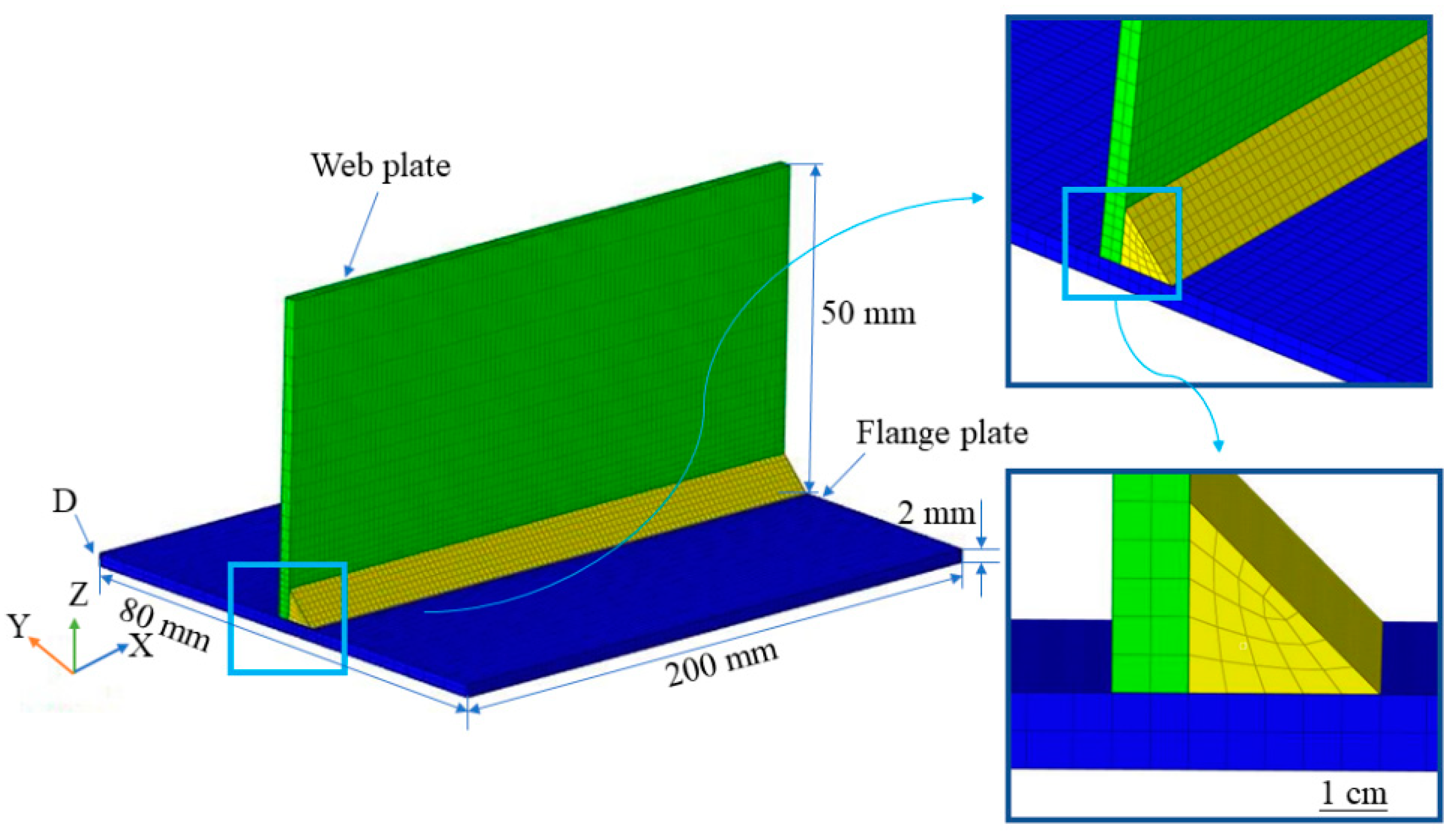
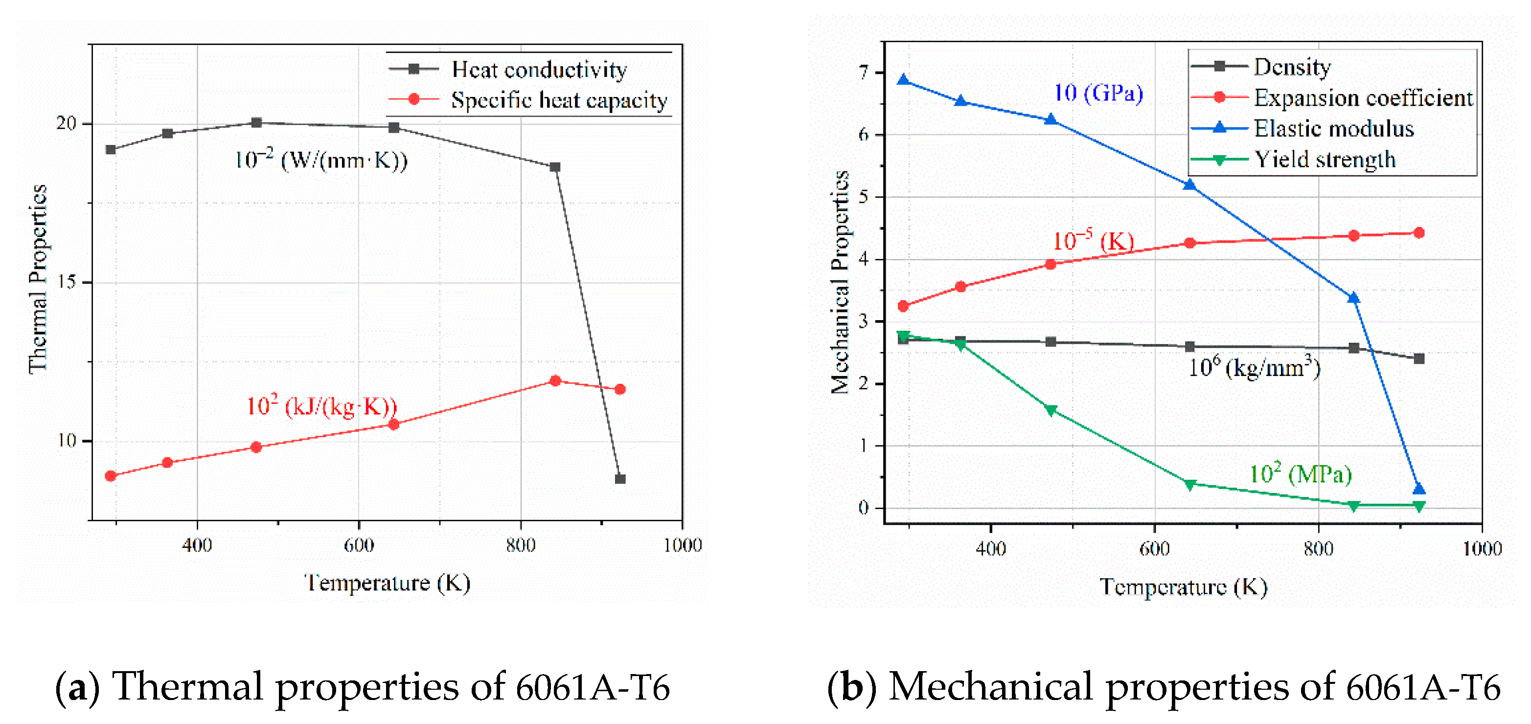
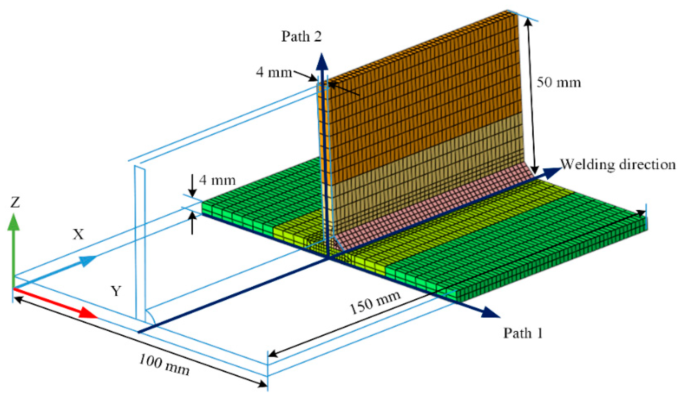
2. Finite Element Simulation

A T-joint FE model is established for this study using Hypermesh. The dimensions of the web plate and flange plate are 200 mm, 80 mm, and 2 mm; 200 mm, 50 mm, and 2 mm respectively, as shown in Figure 1. Many hexahedron elements and a few tetrahedron elements are adopted in the FE model to assure the quality of grids in the region of the welding seams. To reduce the computation cost, the mesh size of elements in the region of the welding seam and the weld heat-affected zone were set as 1 mm, and the mesh size of elements far away from the above region increased to 5 mm gradually. The numbers of elements and nodes are 13,900 and 20,099, respectively.

The chemical composition of 6061A-T6 is shown in

Table 1. Chemical composition of 6061A-T6 (wt.%).

Mg	Si	Fe	Cu	Cr	Mn	Zn	Ti	Al
0.8–1.2	0.4–0.8	0.70	0.15–0.40	0.04–0.35	0.15	0.25	0.15	Balance

. The temperature-dependent thermal and mechanical properties of 6061-T6 are obtained by reference [27] and the extrapolation method, as shown in Figure 2. The thermal and mechanical properties of the welding seam are equivalent to the thermal and mechanical properties of the region far from the welding seam.

To solve the problem of difficulty in convergence in welding simulation analysis, the sequential thermomechanical coupling method is adopted in this paper. First, the temperature field is analyzed, and then the results of the temperature field analysis are loaded into the stress field as initial conditions for the stress field analysis.

In thermal analysis, the element attribute is Solid 70. Initial condition: set the environment temperature as 293 K. Temperature field boundary conditions: the heat source function model proposed by Goldak et al. [28] with double-ellipsoidal distribution was adopted to simulate the welding process of MIG welding. The heat source distribution of the two ellipsoids is shown in Equations (1) and (2), and the heat transfer coefficient is loaded on the free surface of the model. The application of the moving heat source is realized by the moving welding heat source method [29]. The welding process of metal gradually filled is simulated by the birth-death method [30].

$$q_f(x,y,z)=\frac{6\sqrt{3}{f}_{f}Q}{a_{f}bc\pi \sqrt{\pi }}\exp \left(-3\left(\frac{x^2}{a_f^2}+\frac{y^2}{b^2}+\frac{z^2}{c^2}\right)\right)$$

(1)

$$q_b(x,y,z)=\frac{6\sqrt{3}{f}_{b}Q}{a_{b}bc\pi \sqrt{\pi }}\exp \left(-3\left(\frac{x^2}{a_b^2}+\frac{y^2}{b^2}+\frac{z^2}{c^2}\right)\right)$$

(2)

where a_f, a_b, b, and c are the shape parameters of the heat input, respectively; Q is the thermal input power; f_f is the energy distribution coefficient of the front half of the ellipsoid; and f_b is the energy distribution coefficient of the back half of the ellipsoid. In general, f_f = 0.4 and f_b = 1.6, which are employed for the analysis optimization. According to the shape and size of the weld pool and the temperature field in the actual welding, the shape parameters of the heat source are adjusted and the corresponding model parameters of the double ellipsoid heat source are a_f = 2 mm, a_r = 3.5 mm, b = 2.2 mm, and c = 2 mm.

In mechanical analysis, the element attribute is Solid 185. Initial condition: the results of the temperature field analysis are set as initial conditions. Stress field constraint constraints: all freedom of element D was constrained in Figure 1 to guarantee the convergence of FE calculation.

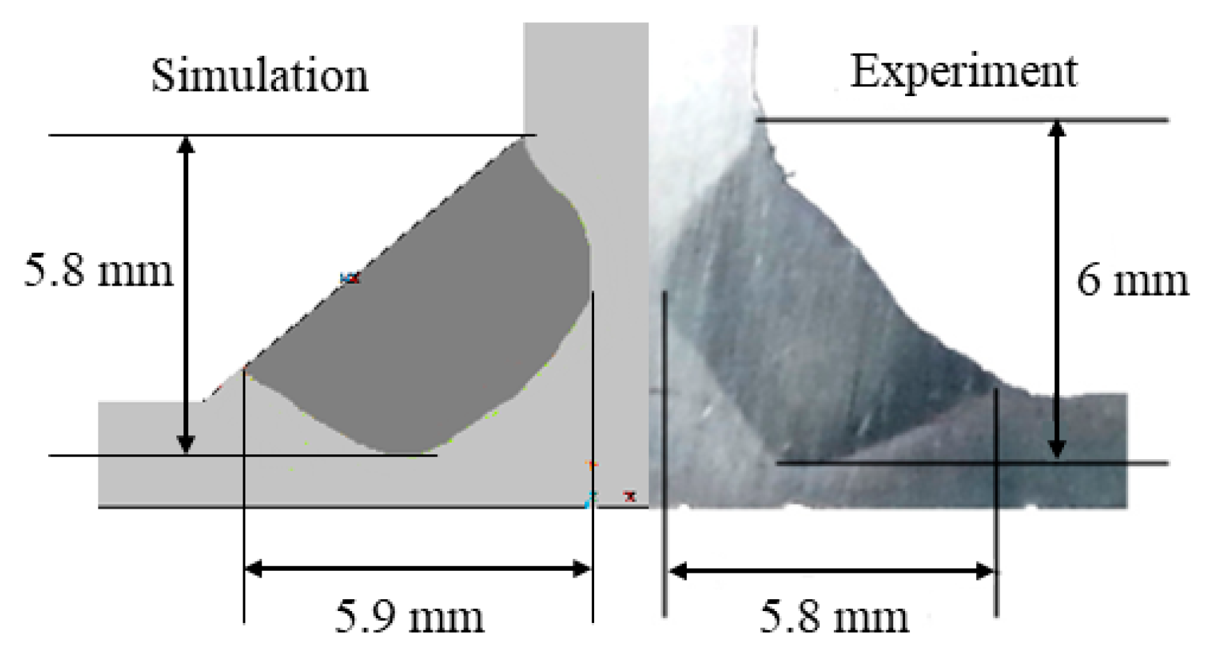
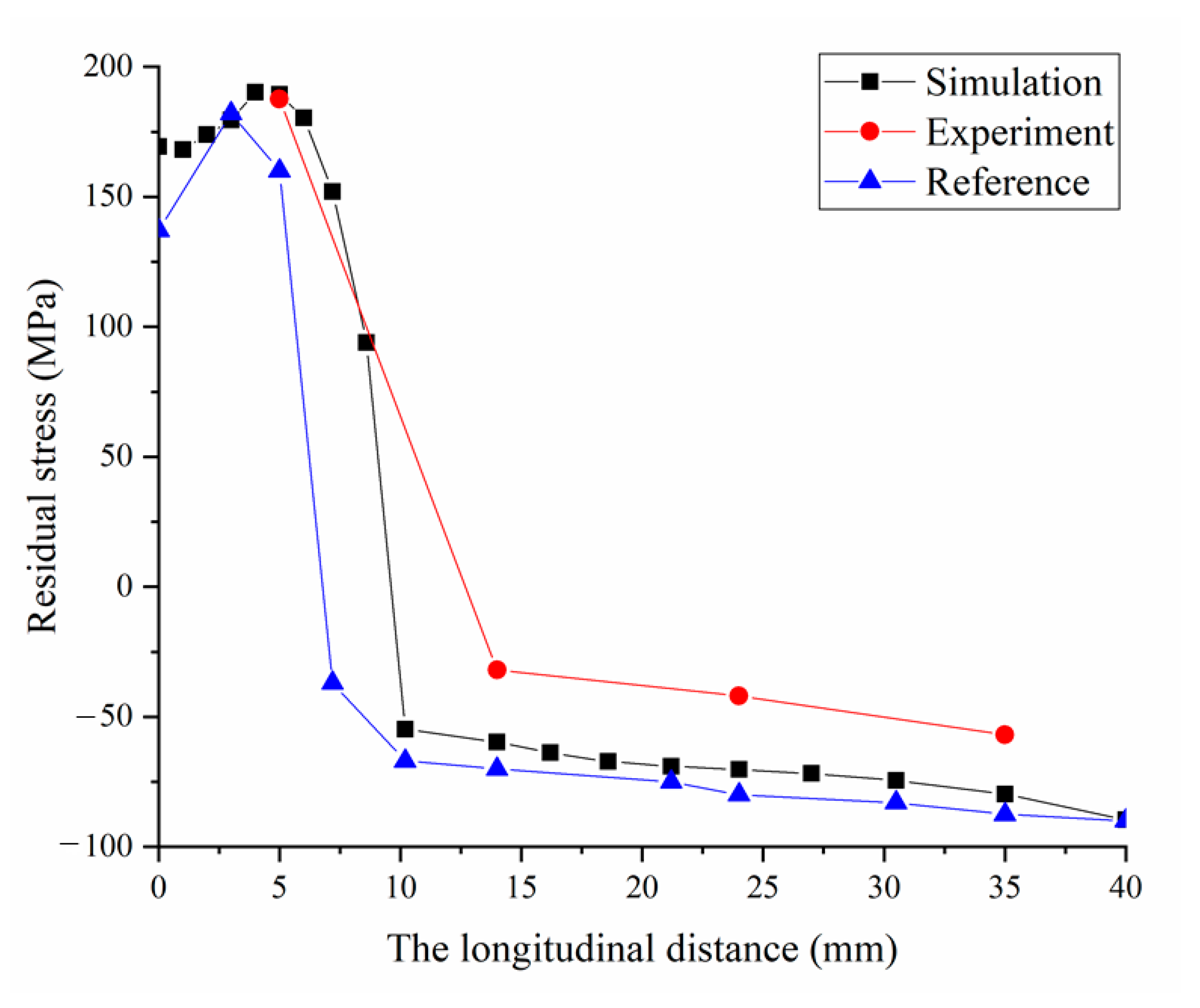
3. Experiments and Finite Element Model Validation

Both the temperature fields and the stress fields were verified according to reference [27] to verify the accuracy of the finite element model. In the experiment, the base material was 6061-T6 Al alloy. The arc welding robot system, produced by OTC in Japan is used for T-joint MIG welding. The filler wire adopted was ER5356 Al-Mg alloy with a diameter of 1.2 mm, and the feed rate of filler wire is 6 m/min. The welding process throughout this work was shielded by pure argon at air flow rate of 25 L/min in the experiment. The welding process parameters of both the experiment and the simulation are welding current 90 A, welding speed 60 cm/min, and welding angle 45°.

According to reference [27], the layout of the measuring points of the web near the fusion zone is shown in Figure 3, each having a length of 5 mm, were installed at points A, B, and C. As shown in Figure 4, the time–temperature curves of experimental measurements and simulation results are highly fitted. Curve A reaches the highest temperature because point A is closest to the welding seam. In addition, the isotherm corresponding to the melting of the base metal is compared with the weld pool shape obtained by the experiment with the same parameters, as shown in Figure 5, verifying the accuracy of the result by simulation.

The residual welding stress of the workpiece was measured by the blind hole method. Four strain gauges of 10 mm were located on the flange plate, from 1 to 4. Welding residual stress and deformation comparison of the experimental measurements and simulation results of this paper and the simulation result of reference [27] are shown in Figure 6 and

Table 2. Comparison of simulated and experimental results of welding deformation of T-joint.

Result	Experiment [27]	Simulation	Deviation	Simulation [27]	Deviation
Distance along Z direction (mm)	1.1	1.08	1.8%	1.05	4.5%
Angular deformation (°)	1.61	1.54	4.3%	1.50	6.8%

, respectively. As shown in Figure 6, the welding stress curves of the experimental measurements and simulation results are highly fitted. Furthermore, the deviation of welding deformation between the simulation in this paper and experimental values is smaller than the deviation between the simulation in reference [27] and experiment values, which illustrates the effectiveness and high accuracy of the simulation method in this paper.

4. Multi-Objective Optimization Problem

Among the different kinds of ANN, the back-propagation neural network (BPNN) [31] was selected for its strong nonlinear relationship identification ability in finding the complex nonlinear relationship between welding process parameters and welding deformation in multiple groups of welding samples. This nonlinear relation is then used to predict the welding deformation and stress of the combination of several alternative welding parameter samples and establishes the objective functions of the multi-objective optimization problem.

4.1. Selection of the Process Parameter Combination Based on OLHS

Many process parameters affect the welding effect in MIG welding, such as welding current, welding voltage, welding speed, and shielding gas flow rate. To reduce welding cracks, welding residual tensile stress, and ensure the depth of fusion, it is necessary to preheat thick welding parts before welding and to reasonably control the welding heat input. Therefore, the welding process parameters, preheat temperature, preheat area, welding speed, and welding heat input, which are effective in solving the above problem, are set as the research objects.

In the welding process of aluminum alloy, the welding heat input and preheat temperature must be strictly controlled to ensure the welding quality. If the preheat temperature is too low, the preheating effect before welding cannot be achieved. If the preheat temperature is too high, the performance of the aluminum alloy may be affected, leading to joint softening and the formation of a weld with a bad appearance. To prevent excessive local stress, the range of preheating must be no less than three times the thickness of the welded part on both sides of the weld and no more than 100 mm.

Furthermore, if the welding heat input is too low and the welding speed is too fast, the welding arc will be unstable and will cause defects such as incomplete welding and slag clamping. However, when the welding heat input is too high and the welding speed is too slow, defects such as burn-through, bite edge, and coarse grain in the heat-affected zone will easily occur, affecting the mechanical properties of the welding seam. Thus, as shown in

Table 3. The range of research parameters.

Research Parameters	Selected Range
Preheat temperature	80–125 °C
Preheat area	12–36 mm
Welding speed	7.5–9 mm/s
Welding heat input	1500–1700 W

, the range of research parameters is selected according to the material, welding method, thickness of the welding plate, and welding procedure specification.

Among many alternative combinations of welding process parameters, the set of combinations that can achieve the optimization goal is selected as the optimal plan. The spare set is the solution space of this welding process parameter optimization system. Therefore, the greater the number of alternative welding process parameter combinations, the larger the optimization space and the greater the possibility of obtaining the optimal combination. However, if all the combinations are listed, there are many redundant plans, which seriously affects the operational efficiency of the system.

Thus, OLHS [32] is utilized to generate samples within the design space. Preheat temperature, preheat area, welding speed, and welding input were chosen as the four factors, and for each factor, four levels were chosen. The total of all the process parameter combinations is 4⁴, but the OLHS table only requires 72 combinations to completely reflect the basic situation.

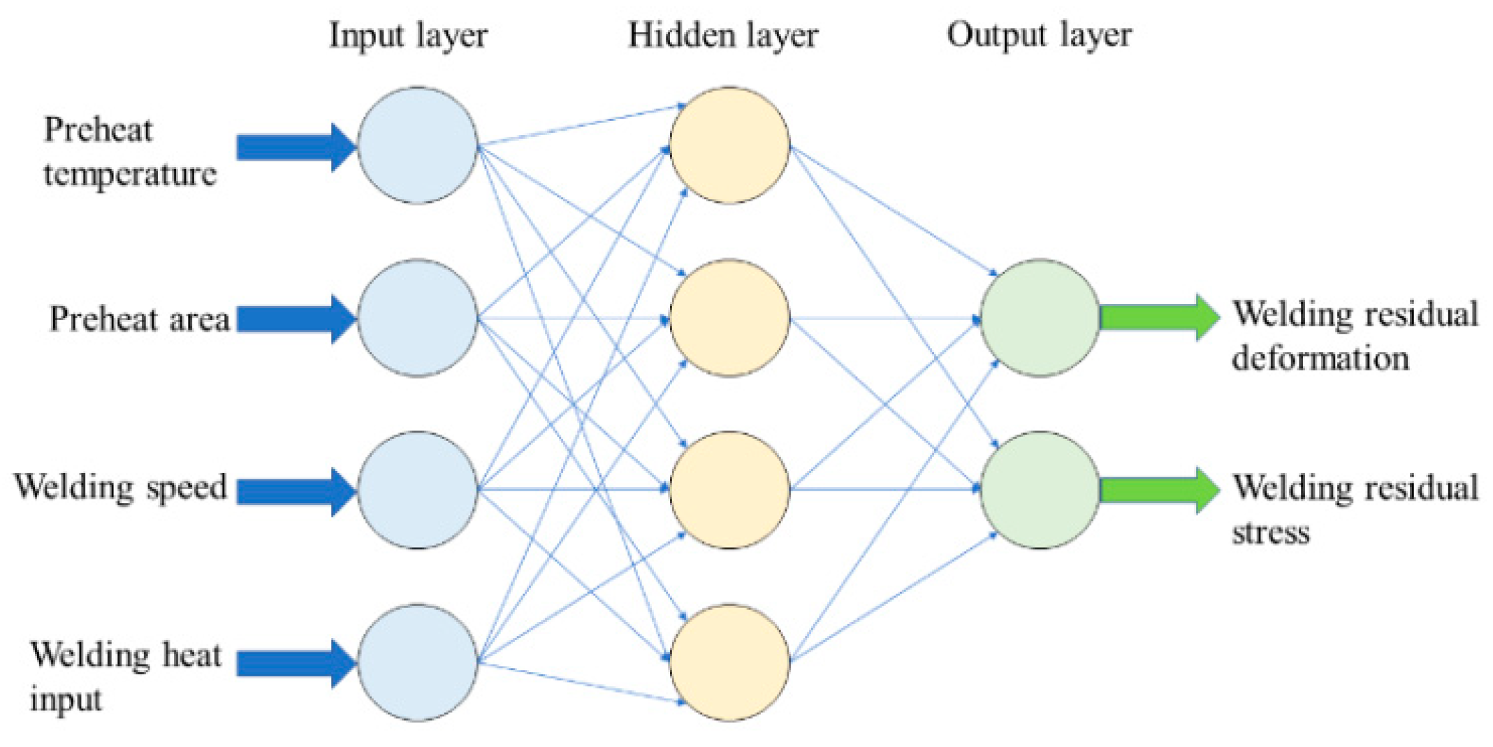
4.2. Design of a Back-Propagation Neural Network

A three-layer BPNN structure was chosen as the prediction model. The numbers of neurons in the input layer and the output layer were four and one, respectively. Each neuron of the input layer represents welding current, welding voltage, welding speed, and preheat temperature. Welding deformation and welding stress were chosen as the output layer neuron to establish two four-input and one-output BPNN structure, respectively.

According to the formula, the number range of hidden layer neurons was calculated. Then, comparing the performance of BPNN under different hidden layer neurons, the number of neurons that could cause the performance of BPNN to reach the best prediction performance was found.

$$hidden\_num=\sqrt{m+n}+a$$

(3)

where hidden_num is the neuron number of the hidden layer, m and n are the neuron numbers of the input layer and output layer, and a is an integer between 0 and 10. The number of hidden layer neurons was set as an integer between 2 and 13 to train the network. According to the mean square error (MSE) value obtained in each training, it is found that when the number of hidden layer nodes is 6, the MSE value trained by the network is the smallest and the network performance is the best. Therefore, the network structure of this model is finally determined as 4-6-1, as shown in Figure 7.

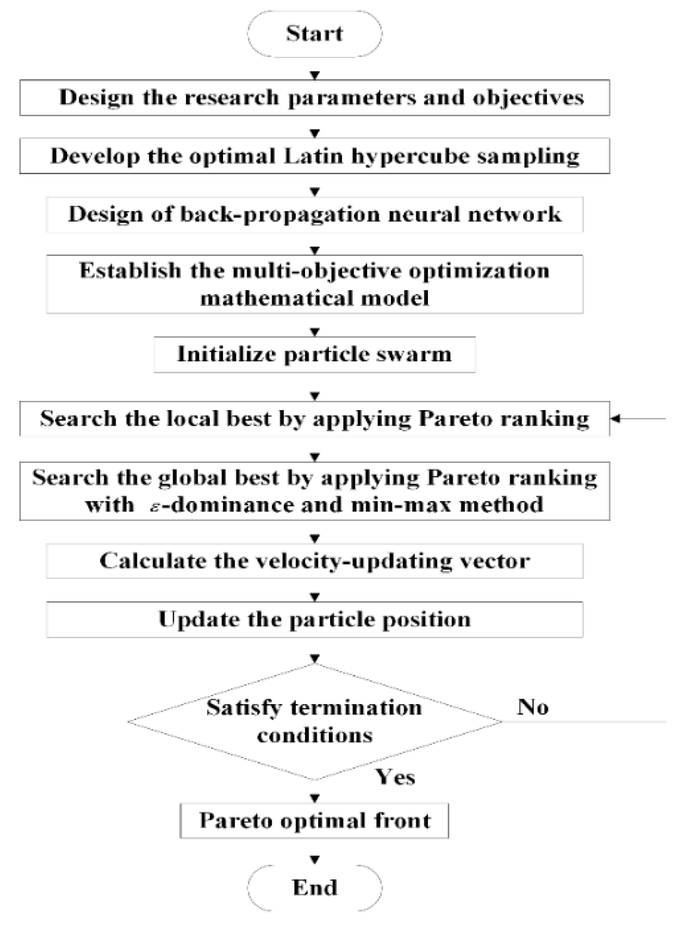
4.3. Multi-Objective Particle Swarm Optimization Algorithm

4.3.1. Definition of Optimization

The prediction model of welding deformation and welding stress is equivalent to the objective function of the multi-objective optimization model. In this model, the optimization variable is the set of welding process parameters, and the objective variables are welding deformation and welding stress. The functional relation between the optimization variable and the objective variable Y_{Welding residual deformation}, Y_{Welding residual deformation} = f(X_{Preheat temperature}, X_{Preheat area}, X_{Welding speed}, X_{Welding heat input}) is the nonlinear relation gained by the BPNN algorithm based on sample data. The constraint condition of optimization variable X is determined according to the welding equipment and product quality. The value range of each optimization variable in this paper is shown in Equation (4). The multi-objective optimization mathematical model of welding process parameter is established as follows:

$$\begin{array}{l}find:\hspace{0.17em}X=\left(X_{\mathrm{Preheat}\mathrm{temperature}},X_{\mathrm{Preheat}\mathrm{area}},X_{\mathrm{Welding}\mathrm{speed}},X_{\mathrm{Welding}\mathrm{heat}\mathrm{input}}\right)\\ \min :\hspace{0.17em} Y_{\mathrm{Welding}\mathrm{residual}\mathrm{deformation}}(X),Y_{\mathrm{Welding}\mathrm{residual}\mathrm{deformation}}(X)\\ s.t.\hspace{0.17em}\hspace{0.17em}\hspace{0.17em}\hspace{0.17em}80{\hspace{0.17em}}^{\circ }\mathrm{C}<X_{\mathrm{Preheat}\mathrm{temperature}}<125{\hspace{0.17em}}^{\circ }\mathrm{C}\\ \hspace{0.17em}\hspace{0.17em}\hspace{0.17em}\hspace{0.17em}\hspace{0.17em}\hspace{0.17em}\hspace{0.17em}\hspace{0.17em}12\hspace{0.17em}\mathrm{mm}<X_{\mathrm{Preheat}\mathrm{area}}<36\hspace{0.17em}\mathrm{mm}\\ \hspace{0.17em}\hspace{0.17em}\hspace{0.17em}\hspace{0.17em}\hspace{0.17em}\hspace{0.17em}\hspace{0.17em}\hspace{0.17em}45\hspace{0.17em}\mathrm{cm}/\min <X_{\mathrm{Welding}\mathrm{speed}}<\hspace{0.17em}54\hspace{0.17em}\mathrm{cm}/\min \\ \hspace{0.17em}\hspace{0.17em}\hspace{0.17em}\hspace{0.17em}\hspace{0.17em}\hspace{0.17em}\hspace{0.17em}\hspace{0.17em}1500\hspace{0.17em}\mathrm{W}\text{<}{X}_{\mathrm{Welding}\mathrm{heat}\mathrm{input}}<1700\hspace{0.17em}\mathrm{W}\end{array}$$

(4)

where $Y_{\mathrm{Welding}\mathrm{residual}\mathrm{deformation}}(X),Y_{\mathrm{Welding}\mathrm{residual}\mathrm{deformation}}(X)$ are the optimization objective functions, which are replaced by the prediction model in the actual optimization, Y_{Welding residual deformation} and Y_{Welding residual deformation} represent the welding deformation and welding stress predicted by the prediction model, respectively.

4.3.2. The Pareto Front

It is difficult for each optimization objective to reach the optimal solution simultaneously, hence the Pareto optimal solution is usually discussed in the multi-objective optimization problem. In Pareto optimal solutions, a set of solutions is created such that none is dominant to the others.

5. Results and Discussion

5.1. Results of OLHS Table

According to the OLHS method and the selected range of the research parameters, 72 combinations of different values of each parameter are listed in

Table 4. OLHS Plans and Results.

No	Optimization Variable				Objective Variable
	Preheat Temperature (X1) (°C)	Preheat Area (X2) (mm)	Welding Speed (X3) (mm/s)	Welding Heat Input (X4) (W)	Heat Source Central Temperature (°C)	Welding Residual Deformation (Y1) (mm)	Welding Residual Stress (Y2) (MPa)
1	95	20	8.5	1570	1091	1.904	186.36
2	95	20	9	1700	1150	1.926	181.74
3	95	36	7.5	1700	1320	2.002	129.12
4	95	36	9	1630	1125	1.929	173.30
5	95	12	8	1700	1207	1.896	171.43
6	95	28	8.5	1700	1206	1.962	165.51
7	95	36	8	1500	1105	1.917	171.88
8	95	28	7.5	1570	1189	1.951	159.43
9	95	20	7.5	1500	1115	1.909	176.34
10	95	20	8	1630	1177	1.925	171.97
11	95	12	8.5	1630	1113	1.873	185.90
12	95	12	9	1570	1011	1.860	199.86
13	80	36	9	1700	1154	1.910	173.22
14	80	20	8.5	1500	1004	1.879	197.36
15	80	28	9	1500	974	1.880	198.75
16	80	20	8	1700	1216	1.910	167.56
17	80	36	7.5	1630	1227	1.920	148.05
18	80	12	7.5	1500	1074	1.851	184.19
19	80	28	8.5	1630	1137	1.905	179.16
20	80	20	7.5	1700	1265	1.932	155.23
21	80	28	7.5	1570	1169	1.916	166.15
22	80	12	8.5	1700	1158	1.867	181.54
23	80	36	8	1500	1080	1.888	178.16
24	80	28	8	1630	1175	1.918	169.41
25	110	20	9	1500	1000	1.915	198.42
26	110	36	9	1630	1148	1.964	166.27
27	110	36	8.5	1700	1241	2.000	145.53
28	110	12	9	1700	1137	1.900	185.61
29	110	28	9	1570	1090	1.959	182.17
30	110	20	8.5	1570	1109	1.932	183.01
31	110	12	8	1630	1166	1.901	176.75
32	110	36	7.5	1570	1225	1.984	137.67
33	110	28	7.5	1630	1266	2.013	141.98
34	110	20	7.5	1700	1305	2.001	144.46
35	110	28	8	1500	1117	1.956	173.91
36	110	12	8.5	1500	1009	1.870	198.54
37	80	12	8	1570	1095	1.855	185.84
38	80	28	7.5	1500	1113	1.901	174.49
39	80	28	9	1700	1147	1.916	178.30
40	80	36	8	1570	1140	1.901	169.89
41	80	36	9	1500	983	1.876	192.99
42	80	12	9	1630	1054	1.853	196.78
43	80	12	8	1630	1146	1.864	180.61
44	80	20	8	1500	1054	1.874	188.68
45	80	12	7.5	1700	1243	1.892	162.00
46	80	20	7.5	1630	1203	1.910	165.84
47	80	20	9	1570	1023	1.873	197.44
48	80	36	8.5	1570	1097	1.892	178.84
49	125	12	9	1700	1149	1.919	183.76
50	125	36	8	1630	1259	2.027	132.03
51	125	28	8	1700	1305	2.066	137.49
52	125	28	9	1500	1056	1.979	183.51
53	125	20	8.5	1630	1170	1.979	173.84
54	125	20	9	1630	1132	1.971	182.26
55	125	20	7.5	1570	1203	1.982	160.36
56	125	20	8.5	1700	1222	1.998	167.41
57	125	20	8	1570	1164	1.971	171.76
58	125	28	7.5	1630	1291	2.055	134.07
59	125	36	7.5	1500	1188	1.998	138.36
60	125	36	9	1570	1127	1.984	164.14
61	125	12	7.5	1570	1168	1.918	172.15
62	125	28	8.5	1500	1099	1.983	176.19
63	125	28	9	1630	1156	2.011	171.14
64	125	12	9	1500	976	1.884	202.62
65	125	12	8	1500	1070	1.894	188.02
66	125	36	8.5	1630	1209	2.013	144.84
67	125	12	7.5	1630	1217	1.932	164.90
68	125	28	8	1570	1189	2.013	156.82
69	125	36	8	1700	1321	2.061	123.87
70	125	12	8.5	1570	1089	1.898	189.93
71	125	28	7.5	1700	1351	2.090	124.79
72	125	20	7.5	1500	1185	1.963	170.15

. To study the influence of the welding heat input and prevent burn-through and excessive deformation, the thickness of the aluminum sheet is increased to 4 mm, as shown in Figure 8. Furthermore, 72 combinations are conducted using the temperature-dependent properties in Figure 2 and the sequential thermomechanical coupling method mentioned in Section 2.

The optimization objectives of welding residual deformation and welding stress only reflect the results in the stress field after thermal-mechanical coupling analysis. Thus, the average central temperature of the heat source is extracted to reflect the rules of welding heat input as a reference in the temperature field after thermal analysis. Finally, the average central temperature of the heat source, the maximum deformation along the Z direction, and maximum welding tensile stress along path 1 are extracted as the result of each combination and are listed in Table 4.

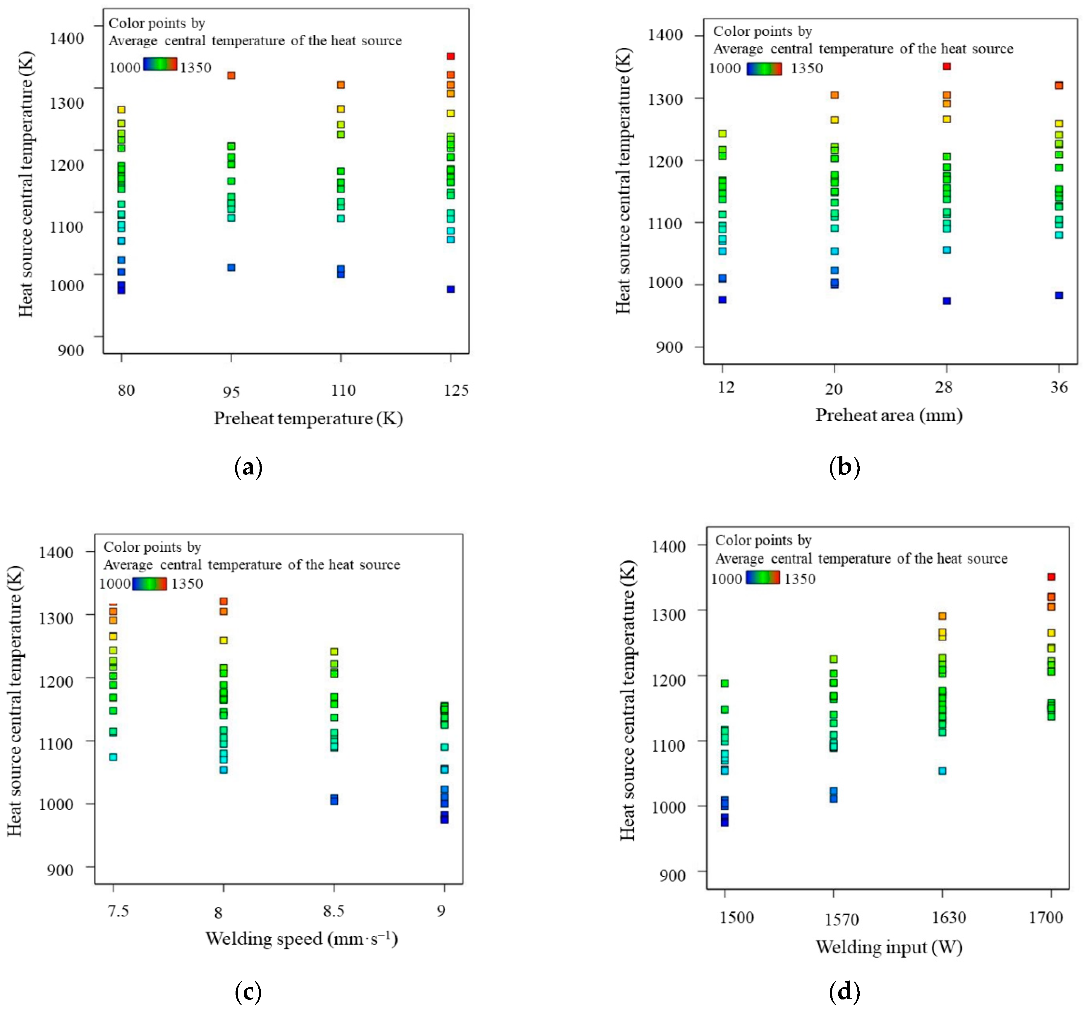
5.2. Influence of Welding Parameters

5.2.1. ANOVA for Heat Source Central Temperature, Welding Residual Deformation and Welding Residual Stress

To further study the influence of the process parameters, the influence degree of each parameter and the ANOVA for heat source central temperature, welding residual deformation, and welding residual stress are discussed in this section according to the results listed in Table 4.

The influence of different process parameters on the average central temperature of the heat source is shown in Figure 9. By and large, the preheat temperature, preheat area, and welding input are positively correlated with the heat source central temperature and welding heat input, and the welding speed is a negative correlation with the target, as shown in Figure 9a–d. This indicates that the higher the total welding heat input per unit time and unit area, the higher the central temperature of the heat source will be.

The influence of different process parameters on welding residual deformation and stress is shown in Figure 10. Generally, the higher the heat input, the larger the residual deformation caused by temperature change. Because the deformation releases some stress, the larger the deformation is, the smaller the residual stress. As shown in Figure 10a–d, the overall trend is the same as the above theory, but some points do not satisfy. That is probably because preheating raises the temperature around the weld seam, and an appropriate preheat temperature and preheat zone can reduce the temperature change gradient to reduce the welding tensile stress. Thus, it is necessary to further discuss the influence degree of each variable on the analysis target to find the influence of this parameter on the temperature field and stress field and the best value of this parameter to control the residual stress according to the actual demand in production.

To find the influence degree of each variable, the ANOVA is shown in

Table 5. The ANOVA for heat source central temperature, welding residual deformation and stress.

Source	Heat source Central Temperature			Welding Residual Deformation			Welding Residual Stress
	F-Value	p-Value	–	F-Value	p-Value	–	F-Value	p-Value	–
Preheat temperature (A)	883.33	<0.0001	significant	11,116.15	<0.0001	significant	239.05	0.0113	–
Preheat area (B)	515.71	<0.0001	significant	4272.88	<0.0001	significant	3955.25	<0.0001	significant
Welding speed (C)	2400.74	<0.0001	significant	651.98	<0.0001	significant	4302.08	<0.0001	significant
Welding input (D)	4125.25	<0.0001	significant	2105.38	<0.0001	significant	3097.19	<0.0001	significant
AB	16.61	0.0032	–	181.84	<0.0001	significant	166.65	0.0007	–
AC	1.17	0.4567	–	7.1	0.022	–	7.9	0.059	–
AD	0.4833	0.8381	–	23.23	0.0015	–	7.24	0.0676	–
BC	1.43	0.3613	–	11.75	0.0072	–	21.29	0.0153	–
BD	0.6517	0.7286	–	25.66	0.0012	–	11.12	0.0366	–
CD	1.33	0.3961	–	27.01	0.001	–	20.04	0.0165	–

based on the OLHS plans and results. The F-value reflects the influence degree on the heat source central temperature, welding residual deformation, and welding residual stress, respectively. The greater the F-value is, the greater the correlation. The p-value reflects the significance level of the parameters. If the p-value is less than 0.0001, this parameter has a significant effect on the result. AB, AC, and so on in the first column reflect the effect of the interaction of the two parameters on the result.

It can be seen from Table 5 that all the process parameters have a significant effect on the heat source central temperature, but the welding input has the greatest impact. However, for welding residual deformation, the preheat temperature and area have the greatest impact. Furthermore, the welding speed and preheat area greatly affect the residual stress, and the preheat temperature has no significant effect on the residual stress.

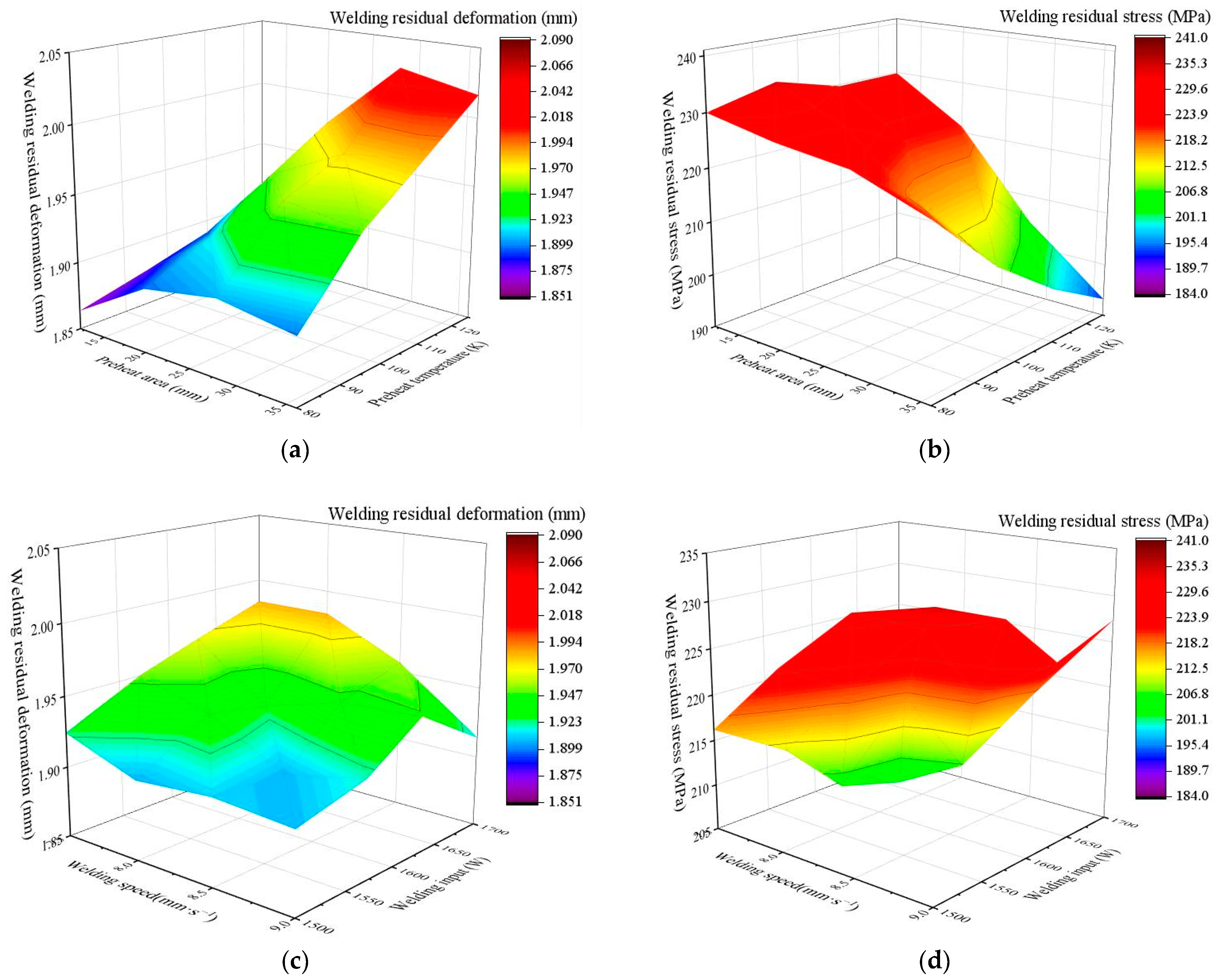
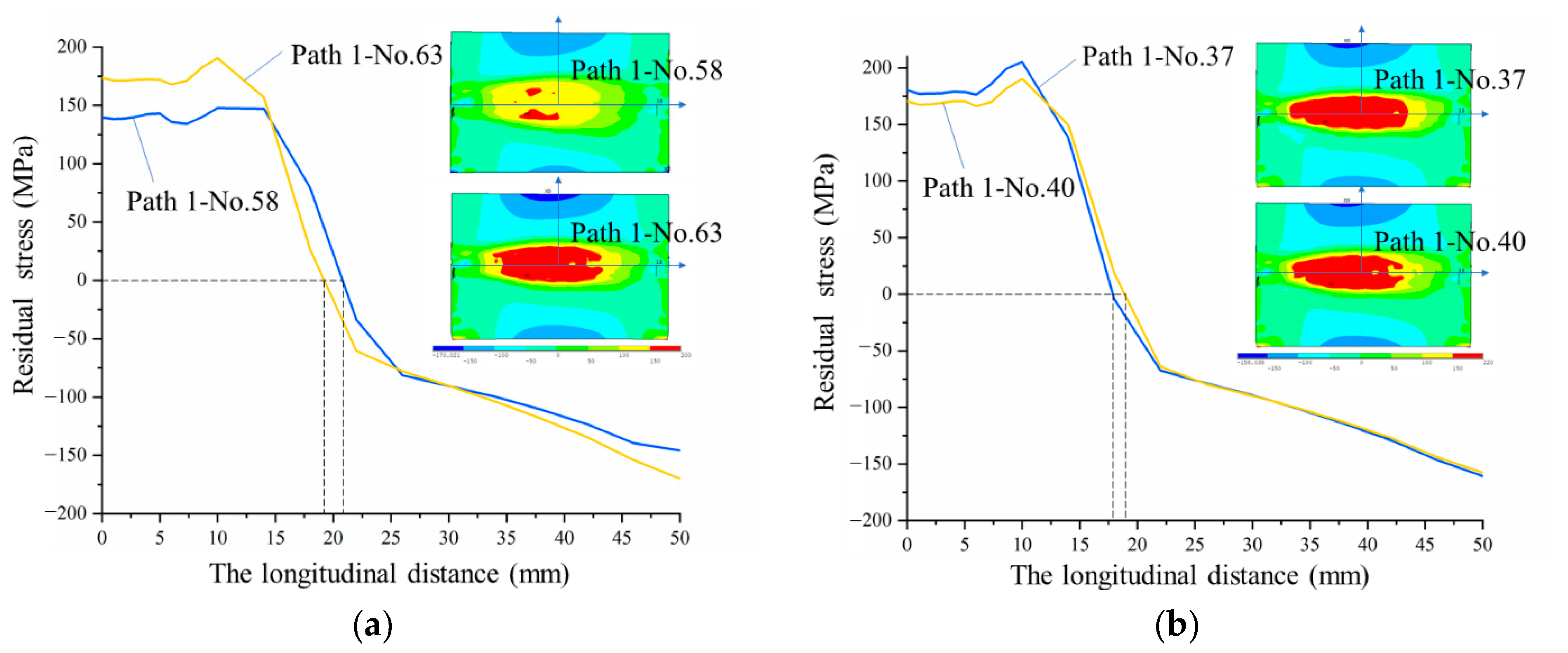
5.2.2. Discussion of Welding Residual Deformation and Stress

According to the conclusion of ANOVA, the preheat temperature has the greatest influence on the residual deformation of the T-joint, and the preheat area has a secondary impact on residual deformation. Thus, the temperature cycle curves of group 15 (preheat temperature 80 °C), group 52 (preheat temperature 125 °C), group 37 (preheat area 12 mm), and group 40 (preheat area 36 mm) were extracted, and the corresponding residual deformation results were discussed.

The temperature curve of the tracking points of different preheat temperatures and preheat areas is shown in Figure 11. It can be seen from Figure 11a–d that the variation trend of the temperature curve at tracking point A and tracking point B is consistent, which shows that the temperature curve first remains unchanged, then rises rapidly, and finally falls rapidly to a stable level. The variation trend of the temperature curve at tracking point C is to remain unchanged at first, then to rise slowly, and finally stabilize. In the 50 s, the temperature curves of all tracking points coincide. In addition, the closer to the weld seam, the higher the maximum temperature and heat input at the tracking point, and the more drastic the temperature change.

It can be seen that the variation trend of the temperature curve at each tracking point is similar. The difference occurs between the maximum temperature at the tracking point and the temperature at the end of the simulation. With the increase in the preheat temperature and preheat area, the welding heat input and final temperature at the same tracking point also increase slightly. Preheating increased the depth of fusion and welding heat input on the outer surface of the weld, reduced the temperature gradient and cooling rate after welding, improved the plastic deformation ability of the material, and reduced the welding stress to prevent the formation of cracks. However, the residual deformation of groups 52 (preheat temperature 125 °C) and 40 (preheat area 36 mm) are 5.27% and 2.48% higher than the values for groups 15 (preheat temperature 80 °C) and 37 (preheat area 12 mm), respectively. Therefore, further optimization analysis is needed to obtain the minimum deformation.

Figure 12 shows the distribution of equivalent residual stress and deformation of T-joints after cooling. Because the transverse stress change is relatively small, this section only considers the longitudinal stress.

According to the conclusion of ANOVA, the effects of welding speed and preheat zone on the residual stress distribution of T-joints are discussed, respectively. The stress curves of group 58 (welding speed 7.5 mm/s) and 63 (welding speed 9 mm/s) were extracted and the corresponding residual stress results were discussed. As shown in Figure 12a, the faster the welding speed is, the lower welding heat input is, the higher the welding residual stress is, but the wider the distribution of welding residual compressive stress is.

As shown in Figure 12b, the stress curves of groups 37 (preheat area 12 mm) and 40 (preheat area 36 mm) were extracted and the corresponding residual stress results were discussed. The wider the preheat zone, the higher welding heat input is, the lower the welding residual stress, but the wider the residual tensile stress distribution. The simulation results showed that preheating can reduce the longitudinal residual stress near the welding beam. However, the wider preheat area can increase the area of tensile stress, which is not good for the fatigue strength of parts.

In practice, preheating of the base material is often used to improve the welding process and improve the welding quality. The preheat temperature should not be too high or too low. Too high a temperature will affect the welding efficiency, and too low a temperature will produce limited improvement of welding deformation and welding stress, so it is necessary to choose the appropriate preheat temperature.

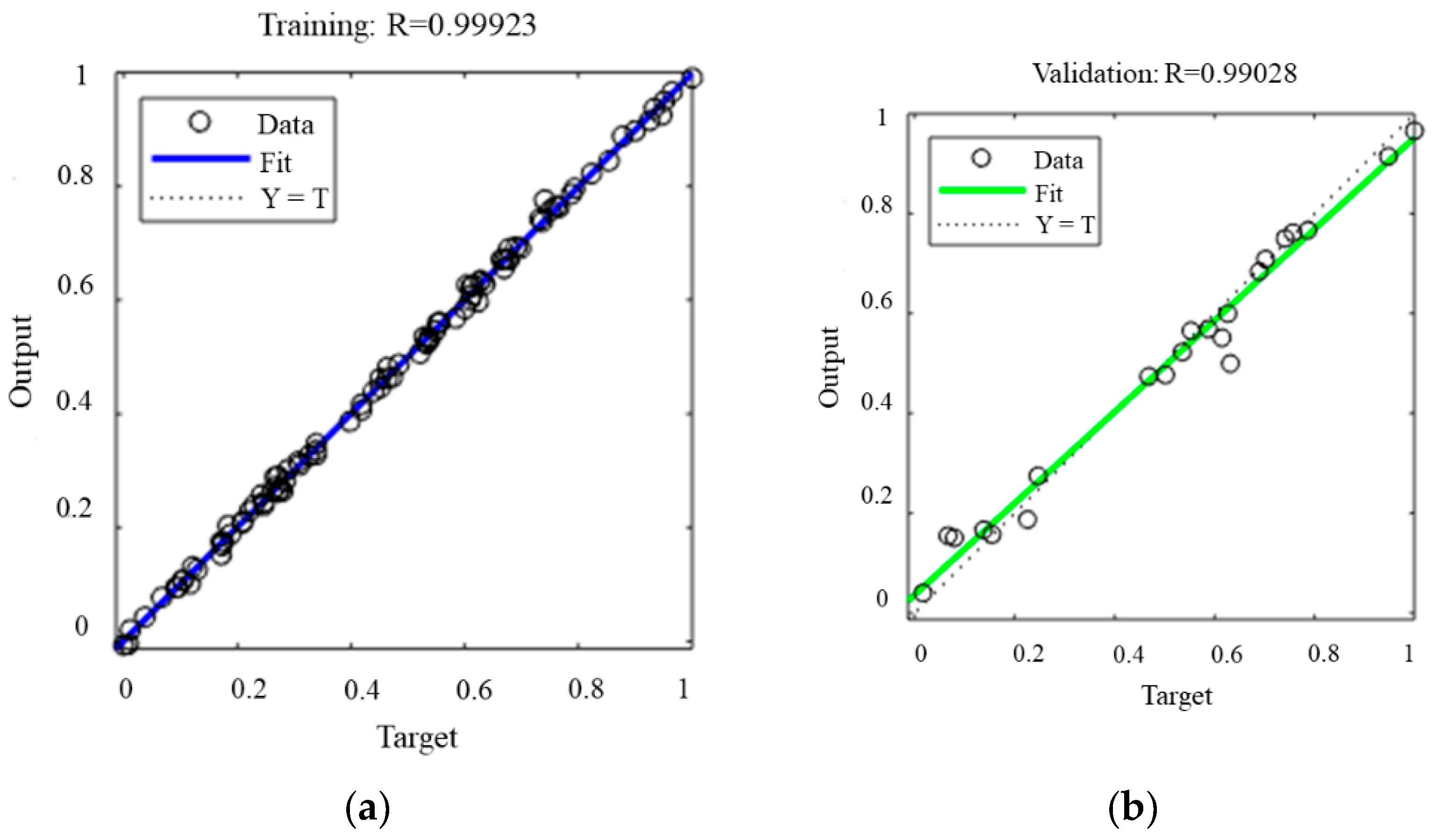
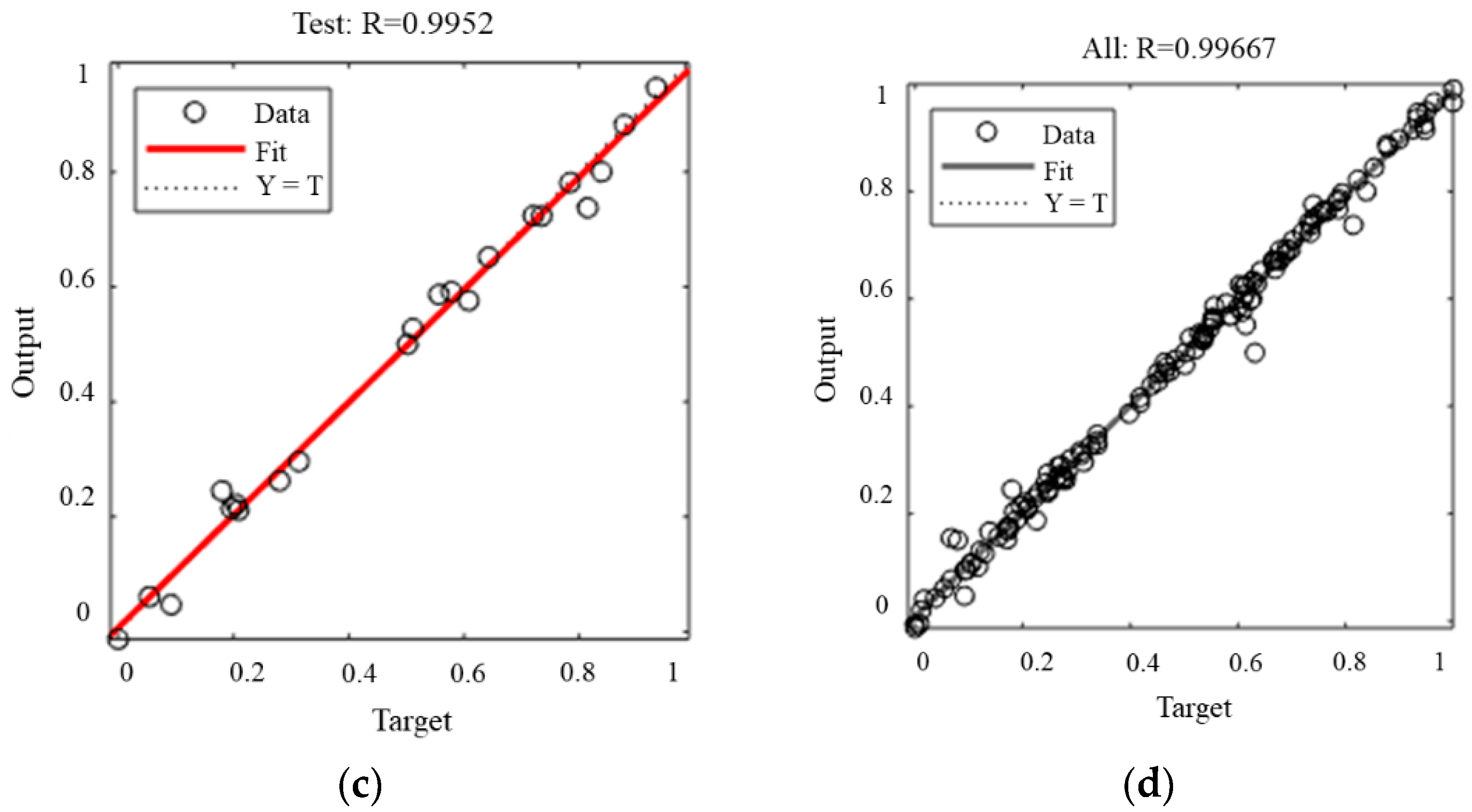
5.3. Performance of BPNN

For further optimization analysis, the BPNN prediction model is established to reflect optimization objectives in this section. To test the BPNN model, the data in Table 4 are separated into 70% training part, 15% validation part, and 15% testing part.

Additionally, the sigmoid function is selected as the transfer function of neurons in the hidden layer and the output layer of the network. MSE is selected as the evaluation index of network performance. The calculation formula of MSE is:

$$MSE=\frac{1}{q}{{\displaystyle \sum _{i=1}^q(y_i-o_i)}}^2$$

(5)

where q, y_i, and o_i represent the number of output neurons, the expected value and predicted value of the ith output neuron, respectively. Figure 13 shows the network error curve, and the least MSE = 0.0019538 illustrates that the BPNN model gains the best validation performance at epoch 12.

The precision distribution of the training and test samples are shown in Figure 13. The aggregation point along the 45° line indicates that the predicted value is close to the true values. The accuracies of the models can be verified by multiple correlation coefficients R. The equation for R is expressed as

$$R=\frac{{\displaystyle \sum _{i=1}^q(y_i-\overline{y})}(o_i-\overline{y})}{\sqrt{{{\displaystyle \sum _{i=1}^q(y_i-\overline{y})}}^2{{\displaystyle \sum _{i=1}^q(o_i-\overline{y})}}^2}}$$

(6)

where y_i is the expected value of the ith output neuron; o_i is the predictive value; $\overline{y}$ is the average of expected values; and q is the number of plans. An R value close to 1 indicates a high degree of coincidence between the origin and the fitting line of the predicted data and a good fitting effect.

As can be observed in Figure 14a, the data points of the training sample were completely coincident with the fitting line (R = 0.999) indicating that the prediction model made full use of the data in the training sample. In Figure 14b,c, the degree of coincidence of data points and fitting lines of the verification samples and the test samples was high, and the R value was 0.990 and 0.995, respectively, indicating that the prediction model had a good prediction effect. Moreover, the difference in R values between the verification samples and the test samples is not large, indicating that the prediction model is relatively robust.

5.4. Optimal Values of Design Parameters for Minimizing Objective Functions

According to the discussion results in Section 5.2, the variation trend of welding residual stress is opposite that of residual deformation. To obtain the solution that meets both the design requirements according to the facts, multi-objective optimization is needed. Based on the BPNN prediction model, the MOPSO algorithm with ε-dominance proposed by Mostaghim et al. [33] is used to optimize the mathematical problem in Section 4.3.1. The MOPSO algorithm [34] was selected to obtain the Pareto front of the objectives for its effective searchability. In addition, the ε-dominance method can find solutions much faster and gain better convergence and diversity. The MOPSO algorithm with ε-dominance only considers the velocity and position variation of the particles when searching the Pareto front, which is more fitted in manufacturing problems. The flowchart of the multi-objective optimization method based on the MOPSO algorithm with ε-dominance is shown in Figure 15.

The initial parameters for the MOPSO algorithm with ε-dominance are as follows: the numbers of population and repository size are both 100; the inertial weight ω is 0.73; the accelerated constants c₁ and c₂ are both 1.5; and the maximum number of iterations Maxygen is 1000. All parameters and results in the optimization domain are normalized to the 0–1 region before optimization. After 950 iterations, the Pareto fronts of the two-objective model are shown in Figure 15. The calculation time in MATLAB was approximately 18.5 s. The 1st objective presents the welding residual deformation, and the 2nd objective presents the welding residual stress. In Figure 16, the star symbol presents the Pareto front to reflect the optimal solutions for different objectives. The Pareto optimal sets are evenly distributed along the Pareto frontier, which indicates that the MOPSO algorithm with ε-dominance has more uniform distribution characteristics.

5.5. Simulation Experiments Confirmation

Three representative optimal solutions were selected from the Pareto front. Case 1 had the minimum value of the 1st objective. Case 2 had the minimum value of the 2nd objective. Case 3 was the compromise solution of the 1st objectives and the 2nd objective. The representative optimal solutions of different objectives are listed in

Table 6. Optimal compromise solution of two-objective optimization models.

No.	Result Type	Preheat Temperature (°C)	Preheat Area (mm)	Welding Speed (mm/s)	Welding Heat Input (W)	Welding Residual Deformation	Welding Residual Stress
Case 1	Optimization	119	33	7.5	1692	0.985	0.616
	FE					0.862	0.665
Case 2	Optimization	81	36	7.6	1653	0.886	1.000
	FE					0.935	0.928
Case 3	Optimization	85	12	8.8	1535	0.927	0.721
	FE					0.881	0.786

. The results indicated that the optimization was consistent with the FE results. The error between the FE results and three representative optimal solutions selected from the Pareto front was less than 12.5%. These compromise solutions help the designers to select appropriate factors for the MIG welding process according to the actual requirements and reduce the dependence on work experience.

6. Conclusions

A validated FE model of 6061-T6 Al alloy T-joint is used to study the influence of welding process parameters and preheat parameters on welding residual deformation and stress. The multi-objective optimization method based on a neural network is adopted to optimize the above parameters to gain the Pareto front. The conclusions of this paper are as follows:

(1)

The thermal elastoplastic method was used to simulate the residual deformation and stress of 6061-T6 aluminum alloy T-joint in ANSYS. The simulation results are basically consistent with the measured data, and the error is within 5%.

(2)

The OLHS and ANOVA method were adopted to sample with uniformity and find the influence degree. The results showed that preheat temperature and welding speed had the greatest effect on the minimization of welding residual deformation and stress, respectively, followed by the preheat area.

(3)

Preheating can reduce the temperature gradient and cooling rate after welding and reduced the welding stress to prevent the formation of cracks. However, the higher the preheat temperature is, the larger the residual deformation is. Furthermore, the simulation results showed that preheating can reduce the longitudinal residual stress near the welding beam. However, the wider preheat area can increase the area of tensile stress, which is not good for the fatigue strength of parts. In addition, the faster the welding speed is, the higher the welding residual stress is, but the wider the distribution of welding residual compressive stress is.

(4)

Artificial neural network-based MOPSO was used to optimize the effective parameters to minimize welding deformation and stress. The BPNN was selected to predict the value of the objective functions. The R values were 0.990 and 0.995, respectively, indicating that the prediction model had a good prediction effect.

(5)

Welding residual deformation and stress are at the minimum at the same time, when the welding parameters are selected as preheating temperature 85 °C and preheating area 12 mm, welding speed 8.8 mm/s and heat input 1535 W, respectively. The Pareto front was obtained by using the MOPSO algorithm with ε-dominance. The error between the FE results and the Pareto optimal compromise solutions is less than 12.5%. The designers can select one solution from many Pareto solutions according to practical needs.

(6)

Further, in order to further verify the reliability of the prediction, we will test and verify the welding results in the test group in the future, and obtain more useful conclusions by comparing the change rules of welding heat curve, residual deformation and stress.

References

1. Zhang, W.; Miao, B. Development trend and prospect of key technologies for next generation high speed trains. Electri. Drive Locomot. 2018, 1, 1–12. [Google Scholar]
2. Yang, S.; Zhang, D.; Tuo, W.; Yu, Z. Microstructures and properties of extruded Al-0.6Mg-0.6Si aluminium alloy for high-speed vehicle. Procedia Eng. 2014, 81, 598–603. [Google Scholar] [CrossRef] [Green Version]
3. Çam, G.; İpekoğlu, G. Recent developments in joining of aluminum alloys. Int. J. Adv. Manuf. Technol. 2017, 91, 1851–1866. [Google Scholar] [CrossRef]
4. Rozumek, D.; Lewandowski, J.; Lesiuk, G.; Correia, J. The influence of heat treatment on the behavior of fatigue crack growth in welded joints made of S355 under bending loading. Int. J. Fatigue 2020, 131, 105328. [Google Scholar] [CrossRef]
5. Yi, J.; Zhang, J.; Cao, S.; Guo, P. Effect of welding sequence on residual stress and deformation of 6061-T6 aluminium alloy automobile component. Trans. Nonferrous Met. Soc. Chin. 2019, 29, 287–295. [Google Scholar] [CrossRef]
6. Shao, Q.; Xu, T.; Yoshino, T.; Song, N. Multi-objective optimization of gas metal arc welding parameters and sequences for low-carbon steel (Q345D) T joints. J. Iron Steel Res. 2017, 24, 544–555. [Google Scholar] [CrossRef]
7. Maneiah, D.; Debashis, M.; Prahlada, R.K.; Brahma, R.K. Process parameters optimization of friction stir welding for optimum tensile strength in Al 6061-T6 alloy butt welded joints. Mate. Today 2020, 27, 904–908. [Google Scholar] [CrossRef]
8. Yang, X.; Chen, H.; Zhu, Z.; Cai, C.; Zhang, C. Effect of shielding gas flow on welding process of laser-arc hybrid welding and MIG welding. J. Manuf. Process. 2019, 38, 530–542. [Google Scholar] [CrossRef]
9. Kumar, S.; Singh, R. Optimization of process parameters of metal inert gas welding with preheating on AISI 1018 mild steel using grey based Taguchi method. Measurement 2019, 148, 106924. [Google Scholar] [CrossRef]
10. Matthew, R.K.; Steven, R.S.; Daniel, C.A.; Jeffrey, F.; Ryan, H. Experimental investigation of linear friction welding of AISI 1020 steel with pre-heating. J. Manuf. Processes 2019, 39, 26–39. [Google Scholar]
11. Aalami-Aleagha, M.E.; Foroutan, M.; Feli, S.; Nikabadi, S. Analysis preheat effect on thermal cycle and residual stress in a welded connection by FE simulation. Int. J. Pres. Ves. Pip. 2014, 114, 69–75. [Google Scholar] [CrossRef]
12. Khoshroyan, A.; Darvazi, A.R. Effects of welding parameters and welding sequence on residual stress and distortion in Al6061-T6 aluminum alloy for T-shaped welded joint. Trans. Nonferrous Met. Soc. Chin. 2020, 30, 76–89. [Google Scholar] [CrossRef]
13. Ashu, G.; Madhav, R.; Anirban, B. Metallurgical behavior and variation of vibro-acoustic signal during preheating assisted friction stir welding between AA6061-T6 and AA7075-T651 alloys. Trans. Nonferrous Met. Soc. Chin. 2019, 29, 1610–1620. [Google Scholar]
14. Zhu, C.; Tang, X.; He, Y.; Lu, F.; Cui, H. Effect of preheating on the defects and microstructure in NG-GMA welding of 5083 Al-alloy. J. Mate. Process. Technol. 2018, 251, 214–224. [Google Scholar] [CrossRef]
15. Asadi, P.; Alimohammadi, S.; Kohantorabi, O.; Fazli, A.; Akbari, M. Effects of material type, preheating and weld pass number on residual stress of welded steel pipes by multi-pass TIG welding. Therm. Sci. Eng. Prog. 2020, 16, 100462. [Google Scholar] [CrossRef]
16. Fallahi, A.; Jafarpur, A.; Nami, M.R. Analysis of welding conditions based on induced thermal irreversibilities in welded structures: Cases of welding sequences and preheating treatment. Sci. Iran 2011, 18, 398–406. [Google Scholar] [CrossRef] [Green Version]
17. Liang, Y.; Wang, M.; Wang, J.; Chen, X.; P, G.E. Effect of pre-heating on residual stress in aluminum alloy joint for healthcare applications. Electr. Weld. Mach. 2015, 45, 54–58. [Google Scholar]
18. Liu, B. The Research of Synchronizing Process of Preheating and Welding for High Strength Steel. Master’s Thesis, Hehai university, Jiangsu, China, June 2016. [Google Scholar]
19. Wu, C.; Kim, J.W. Numerical prediction of deformation in thin-plate welded joints using equivalent thermal strain method. Thin Walled Struct. 2020, 157, 107033. [Google Scholar] [CrossRef]
20. Chang, Y.; Yue, J.; Guo, R.; Liu, W.; Li, L. Penetration quality prediction of asymmetrical fillet root welding based on optimized BP neural network. J. Manuf. Process. 2020, 50, 247–254. [Google Scholar] [CrossRef]
21. Kshirsagar, R.; Jones, S.; Lawrence, J.; Kanfoud, J. Effect of the Addition of Nitrogen through Shielding Gas on TIG Welds Made Homogenously and Heterogeneously on 300 Series Austenitic Stainless Steels. J. Manuf. Mater. Process. 2021, 5, 72. [Google Scholar]
22. Bunaziv, I.; Akselsen, O.M.; Frostevarg, J.; Kaplan, A.F.H. Deep penetration fiber laser-arc hybrid welding of thick HSLA steel. J. Mater. Process. Technol. 2018, 256, 216–228. [Google Scholar] [CrossRef]
23. Moradi, M.; Moghadam, M.K.; Shamsborhan, V.; Beiranvand, Z.M.; Bodaghi, M. Simulation, statistical modeling, and optimization of CO2 laser cutting process of polycarbonate sheets. Optik 2021, 225, 164932. [Google Scholar] [CrossRef]
24. Bai, R.; Guo, Z.; Lei, Z.; Wu, W.; Yan, C. Hybrid inversion method and sensitivity analysis of inherent deformations of welded joints. Adv. Eng. Software 2019, 131, 186–195. [Google Scholar] [CrossRef]
25. Huang, H.; Wang, J.; Li, L.; Ma, N. Prediction of laser welding induced deformation in thin sheets by efficient numerical modeling. J. Mater. Process. Technol. 2016, 227, 117–128. [Google Scholar] [CrossRef]
26. Zhang, W.; Fu, H.; Fan, J.; Li, R.; Xu, H.; Liu, F.; Qi, B. Influence of multi-beam preheating temperature and stress on the buckling distortion in electron beam welding. Mater. Design 2018, 139, 439–446. [Google Scholar] [CrossRef]
27. Yi, J.; Cao, S.; Li, L.; Guo, P.; Liu, K. Effect of welding current on morphology and microstructure of Al alloy T-joint in double-pulsed MIG welding. Trans. Nonferrous Met. Soc. Chin. 2015, 25, 3204–3211. [Google Scholar] [CrossRef]
28. Goldak, J.; Chakravarti, A.; Bibby, M. New finite element model for welding heat sources. Metall. Mater. Trans. B 1984, 15, 299–305. [Google Scholar] [CrossRef]
29. Xu, T.; Liu, G.; Ge, H.; Zhang, W.; Yu, Z. Research for Modeling Heat Source of Dynamic Welding with Local Coordinate Curve Path. J.-L. Univ. (Eng. Tech. Ed.) 2014, 44, 1704–1709. [Google Scholar]
30. Shao, Q.; Xu, T.; Yoshino, T.; Song, N.; Yu, Z. Optimization of the welding sequence and direction for the side beam of a bogie frame based on the discrete particle swarm algorithm. Proc. Inst. Mech. Eng. B-J. Eng. 2018, 232, 1423–1435. [Google Scholar] [CrossRef]
31. Rumelhart, D.E.; Hinton, G.E.; Williams, R.J. Learning representations by back-propagating errors. Nature 1986, 323, 533–536. [Google Scholar] [CrossRef]
32. Montgomery, D.C. Design and Analysis of Experiments, 5th ed.; John Wiley & Sons: New York, NY, USA, 2001. [Google Scholar]
33. Mostaghim, S.; Teich, L. The role of ε-dominance in multi objective particle swarm optimization methods. In Proceedings of the 2003 Congress on Evolutionary Computation, Canberra, ACT, Australia, 8–12 December 2003; IEEE: New York, NY, USA, 2004; Volume 3, pp. 1764–1771. [Google Scholar]
34. Kennedy, J.; Eberhart, R. Particle swarm optimization. In Proceedings of the Winter Simulation Conference, Perth, WA, Australia, 27 November–1 December 1995; IEEE: New York, NY, USA, 1995; Volume 11, pp. 1942–1948. [Google Scholar]
Figure 1. T-joint FE model.
Coatings 11 00998 g001
Figure 2. Temperature-dependent properties for 6061-T6.
Coatings 11 00998 g002
Figure 3. Measuring points of temperature and stress field.
Coatings 11 00998 g003
Figure 4. Temperature–time curve comparison of simulated and experimental results.
Coatings 11 00998 g004
Figure 5. Simulation and experiment comparison of bead width and depth.
Coatings 11 00998 g005
Figure 6. Comparison of simulated and experimental results of welding stress of a T-joint.
Coatings 11 00998 g006
Figure 7. Topology of the designed neural network.
Coatings 11 00998 g007
Figure 8. Diagram of the T-joint used in OLHS plans.
Coatings 11 00998 g008
Figure 9. The influence of different process parameters on the average central temperature of the heat source. (a) The influence of preheat temperature; (b) the influence of preheat area; (c) the influence of welding speed; (d) the influence of welding input.
Coatings 11 00998 g009
Figure 10. The influence of different process parameters on welding residual deformation and stress. (a) Effect of preheat area and preheat temperature on welding residual deformation; (b) effect of preheat area and preheat temperature on welding residual stress; (c) effect of welding speed and welding input on welding residual deformation; (d) effect of welding speed and welding input on welding residual stress.
Coatings 11 00998 g010
Figure 11. Temperature curves of tracking points at different preheat temperatures and areas. (a) Temperature curves of group 15; (b) temperature curves of group 52; (c) temperature curves of group 37; (d) temperature curves of group 40.
Coatings 11 00998 g011
Figure 12. Residual stress curve along path 1 at different welding speeds and areas. (a) Residual stress curves of groups 58 and 63; (b) residual stress curves of groups 37 and 40.
Coatings 11 00998 g012
Figure 13. Network error curve obtained from the performance test with the least MSE.
Coatings 11 00998 g013
Figure 14. Performance of BPNN. (a) Fitting situation of the training group; (b) fitting situation of the validation group; (c) fitting situation of the test group; (d) fitting situation of all groups.
Coatings 11 00998 g014aCoatings 11 00998 g014b
Figure 15. Flowchart of the multi-objective optimization method based on MOPSO algorithm with ε-dominance.
Coatings 11 00998 g015
Figure 16. The Pareto optimal front by the MOPSO algorithm with ε-dominance.
Coatings 11 00998 g016